Consistent-Teacher: Towards Reducing Inconsistent Pseudo-targets
in Semi-supervised Object Detection
-Supplementary Material-

In this supplementary material, we provide additional experimental quantitative results, model size comparison, as well as bounding boxes visualization to further support the effectiveness of our proposed Consistent-Teacher . In addition, we delineate more experimental details, implementation information, and hyper-parameter settings of our method. Our code is also attached for your reference.

1 More details in Consistent-Teacher 

1.1 Inconsistency measurement.

Inconsistency refers to the fact that the pseudo boxes may be highly inaccurate and vary greatly at different stages of training. Therefore, we measure the pseudo-bboxes variation across different training steps. Specifically, we store the checkpoints every 4000 training steps. We then run inference using these checkpoints on a subset with 5000 images from the unlabeled set. The prediction output from the previous checkpoint is then set as GT and we evaluate the mAP of the current checkpoint with the previous predictions. Therefore, a higher mAP implies a more consistent pseudo targets. Then the inconsistency is measured by accumulating $1-mAP$ for these checkpoints to reflect the accumulated effect of noisy targets.

2 Verify the Inconsistency in SSOD

Assignment Inconsistency under Noisy Pseudo Labels. To illustrate that the conventional IOU-based or heuristic label assignment is problematic in SSOD, we intentionally inject random noise to the ground-truth bounding boxes and testify the assignment consistency by quantifying the assignment IOU (A-IOU) of clean and noisy assignments. Suppose a bounding box $b=(x_{1},y_{1},x_{2},y_{2})$ is assigned to a set of $k$ anchors $A=\{a_{1},\dots,a_{k}\}$. We add Gaussian noise to its coordinate with a noise ratio $\rho$, so that $b^{\prime}=(x_{1}+\epsilon_{x_{1}}\times w,y_{1}+\epsilon_{y_{1}}\times h,x_{2}+\epsilon_{x_{2}}\times w,y_{2}+\epsilon_{y_{2}}\times h)$, in which $w$ and $h$ are width and height of the box. $\epsilon_{x_{1}},\epsilon_{y_{1}},\epsilon_{x_{2}},\epsilon_{y_{2}}$ are sampled from a normal distribution $\mathcal{N}(0,\rho)$. The perturbed box $b^{\prime}$ is matched to a new set of $l$ anchors $A^{\prime}=\{a^{\prime}_{1},\dots,a^{\prime}_{l}\}$. The A-IOU is computed as the intersection-of-union between $A$ and $A^{\prime}$. The higher A-IOU score suggests the assignment is more robust to label noise.

We testify the assignment consistency under two scenario. First, we calculate the assignment IOU with different degrees of noise ratio $\rho\in\{0.1,0.2,\dots,0.5\}$ using the final model. Second, we would like to investigate how the assignment consistency change through training. We report the A-IOU at different time of training with a constant $\rho=0.1$. We compare our ASA with IOU-based assigner [ren2015faster, lin2017focal, liu2016ssd] and ATSS assigner [zhang2020bridging] with Mean Teacher RetinaNet baseline on COCO 10%. All modules except for the assignment are kept the same to provide a fair comparison. For both evaluations, we randomly select 1000 images from val2017 to compute the A-IOU. Figure 1 visualize the mean$\pm$std A-IOU between clean and noisy label at different training time and different noise ratio $\rho$. In Figure 1(a), both ATSS and our ASA provides higher A-IOU compared with the broadly applied IOU-based assignment. However, ATSS is still based on heuristic matching rule between label and anchor boxes. ASA, instead, steadily improves itself as the detector becomes more accurate. In Figure 1(b), we see that IOU-based assignment fails to maintain the initial assignment when the large magnitude of noise is introduced in the labels. Given the noisy nature of pseudo label in SSOD, our experiment suggests that IOU-based assignment is incapable of maintaining the assignment consistency in SSOD. In contrast, our ASA strategy still performs well under server noise scenario. This experiment supports our argument that the proposed consistent assignment strategy is robust to label noise in SSOD.

Figure 1: Assignment IOU score between ground-truth and the noisy bounding boxes (a) at different time of training and (b) using different noise ratio.

Table 1: Classification and Regression inconsistency analysis using IOU-Confidence linear regression (LR) error. We also provide the Mean Teacher IOU-Confidence plot on the right.

	LR Standard Error
Mean Teacher	0.109
Consistent-Teacher	0.080

Classification and Regression Inconsistency. We unveil the regression and classification mismatch problem in SSOD by identifying the mismatch between the high-score and high-IOU predictions. We obtain the confidence-IOU pairs on val2017 using Consistent-Teacher and Mean Teacher RetinaNet when trained on COCO 10% data, and analyze the correlation between the two variables. We apply linear regression and measures the standard error to reflect the correlation between confidences and IOUs. Smaller error indicates higher correlation.

Table 1 provides the LR standard error for Consistent-Teacher and Mean Teacher RetinaNet. The right scatter figure displays the confidence-IOU of Mean Teacher. We observe clear cls-reg misalignment on semi-supervised detectors: numerous low-confident predictions possess high IOU score. It indicates that classification confidence does not provides a strong enough clue for an accurate regression result, which give rise to erroneous pseudo-label noise during training. The high LR error of 0.109 with Mean teacher also demonstrates this point. On the contrary, our Consistent-Teacher largely elinimates the mismatch between the two tasks with a lower LR error of 0.080. It supports our arguments that Consistent-Teacher can align the classification and regression sub-tasks and reduce the mismatch in SSOD.

3 Semi-supervised detection results visualization

3.0.1 Qualitative comparison with Baseline.

We further compare the baseline Mean Teacher RetinaNet with our Consistent-Teacher by visualizing the predicted bounding boxes on val2017 under the COCO 10% protocol. In Figure 2, we plot the predicted and ground-truth bounding boxes in Violet and Orange respectively, alongside with the false positive bboxes highlighted in Red.

There are 3 general properties that we could observed in our demonstration.

1. First, Consistent-Teacher fits the situation of crowded object localization better, whereas Mean Teacher often mistakes the intersection of two overlapped objects as a new instance. For example, in the scenes of zebras or sheep, Mean Teacher often gives a false positive output in the overlapping area of the two objects, while Consistent-Teacher largely resolves the inaccurate positioning problem through the adaptive anchor selection mechanism.

2. Secondly, we see that under the semi-supervised setting, the Mean Teacher RetinaNet would either predict the wrong class for the correct location or regress an inaccurate bounding box despite its high classification confidence. For example, birds are sometimes misidentified as airplanes even when the localization is accurate. It is mainly attributed to the inconsistency of classification and regression tasks, i.e. the features required for regression may not be optimal for classification. Consistent-Teacher effectively discriminates similar categories using the FAM-3D to select the features dynamically.

3. Third, Consistent-Teacher embraces higher recall since it is capable of detecting small or crowded instances which Mean Teacher fails to point out. For example, Consistent-Teacher discovers most of the hot dogs on the grill while Mean Teacher neglects most of them.

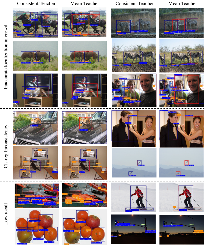
Figure 2: Qualitative comparison on the COCO%10 evaluation. The bounding boxes in Orange is the ground-truth, and Violet refers to the prediction. Red highlights the false positive predictions.

3.0.2 Good cases and Failure cases.

We provides more examples to showcase the good and failure examples produced by Consistent-Teacher on COCO val2017 in Figure 3 and Figure 4. Although our proposed method achieved gratifying performance on a series of SSOD benchmarks, we can still point out its deficiencies in Figure 4. First, the trained detector lacks robustness to some out-of-distribution samples, for example, cartoon characters on street signs are recognized as real people, and reflections in mirrors are recognized as objects. Second, our detection performance is poor for some classes with small sizes, such as toothbrushes, hair dryers, etc. Third, Consistent-Teacher also tends to treat parts of the object as a whole, such as the head of the giant panda as a separate animal (in the lower left corner), and the dial of a clock as the entire clock (on the right of the panda).

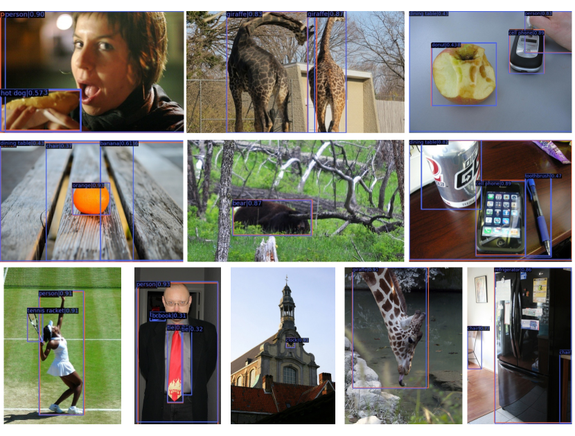
Figure 3: Good detection results for the COCO%10 evaluation. The bounding boxes in Orange is the ground-truth, and Violet refers to the prediction.

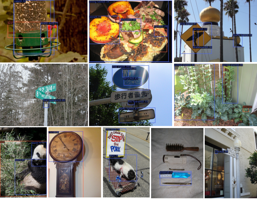
Figure 4: Failure detection results for the COCO%10 evaluation. The bounding boxes in Orange is the ground-truth, and Violet refers to the prediction.

4 Demo Videos

In addition to the static visualizations in the text, we also provide the several demo videos to illustrate the inconsistency problems in SSOD, and how Consistent-Teacher manage to address the them. We provides 3 folder and 1 short video, named Zebra, Giraffa, Polar_Bear, and FAM3D_Selfie.mp4.

The first 3 clip pairs compare the detection bounding boxes between our Mean-Teacher and Consistent-Teacher . The green boxes refer to the gts, red boxes denote the false-positive detections and blues ones for true-positive results. Different frames indicate the detection outputs at different training steps. It is observed that, Mean-Teacher suffers from oscillating detection bboxes and inability to discriminate the adjacent objects. The detection error thus accumulates throughout the training, producing a lot of false-positives. Our Consistent-Teacher addresses the problem by assign the targets with learn-able matching cost, thus largely stabilizes the pseudo bounding boxes, and improves the performance especially under the crowded scene(e.g. Zebra.mp3 and Giraffa.mp4).

The FAM3D_Selfie.mp4 reflects how cls-reg alignment reduces the noisy pseudo-labels. On the right and left, we show the detection results in red with or without the FAM3D head separately. We see that, at late stage of training, a false-positive bbox for “person” pops out in the background on the left, while our model does not. And the full model consistently gets a smaller confidence score during training. In this way, we prevent high-score but low-quality pseudo-bounding boxes from affecting the detectors, resulting in more accurate predictions with less noise.

5 Experiment and Hyper-parameter settings

5.1 Datasets and data prepossessing.

5.1.1 MS-COCO 2017.

The Microsoft Common Objects in Context (MS-COCO) is a large-scale object detection, segmentation, key-point detection, and captioning dataset. We use COCO2017 in our experiments for SSOD, which includes 118K training and 5K validation images along with bounding boxes of 80 object categories.

5.1.2 PASCAL VOC 2007-2012.

The PASCAL Visual Object Classes (VOC) dataset contains 20 object categories alongside with pixel-level segmentation annotations, bounding box annotations, and object class annotations. The official VOC 2007 trainval set is adopted as the labeled set with 5011 images and the 11540 images from VOC 2012 trainval set is used as unlabeled data in this study. We evaluate on the VOC 2007 test set.

5.1.3 Data Augmentations.

We use the same data augmentations as described in Soft Teacher [xu2021end], including a labeled data augmentation in Table 2, a weak unlabeled augmentation in Table 3 and a strong unlabeled augmentation in Table 6.

5.2 Implementation Details

We implement our Consistent-Teacher based on MMdetection framework with the data prepossessing code from the open-sourced Soft-Teacher  and google ssl-detection . We train our detectors on 8 NVIDIA Tesla V100 GPUs. It takes approximately 3 days for an 180K training. Each GPU contains 1 labeled image a and 4 unlabeled images. The source code is attached in a separate zip file.

6 Source Code

All our source code is provided in the Supplementary Material code.zip. Please refer to README.md file for more information.

Table 2: Data augmentation for labeled image training.

Transformation	Description	Parameter Setting
RandomResize	Resize the image to a the height of $h$ randomly sampled from $h\sim U(h_{min},h_{max})$, while keeping the height-width ratio unchanged.	3cm$h_{min}=400,h_{max}=1200$ in MS-COCO
$h_{min}=480,h_{max}=800$ in PASCAL-VOC
RandomFlip	Randomly horizontally flip a image with probability of $p$.	$p=0.5$
OneOf	Select one of the transformation in a transformation set $T$.	$T=$ TransAppearance

Table 3: Weak data augmentation for unlabeled image.

Transformation	Description	Parameter Setting
RandomResize	Resize the image to a the height of $h$ randomly sampled from $h\sim U(h_{min},h_{max})$, while keeping the height-width ratio unchanged.	3cm$h_{min}=400,h_{max}=1200$ in MS-COCO
$h_{min}=480,h_{max}=800$ in PASCAL-VOC
RandomFlip	Randomly horizontally flip a image with probability of $p$.	$p=0.5$

Table 4: Strong data augmentation for unlabeled image.

Transformation	Description	Parameter Setting
RandomResize	Resize the image to a the height of $h$ randomly sampled from $h\sim U(h_{min},h_{max})$, while keeping the height-width ratio unchanged.	3cm$h_{min}=400,h_{max}=1200$ in MS-COCO
$h_{min}=480,h_{max}=800$ in PASCAL-VOC
RandomFlip	Randomly horizontally flip a image with probability of $p$.	$p=0.5$
OneOf	Select one of the transformation in a transformation set $T$.	$T=$ TransAppearance
OneOf	Select one of the transformation in a transformation set $T$.	$T=$ TransGeo
RandErase	Randomly selects $K$ rectangle region of size $\lambda h\times\lambda w$ in an image and erases its pixels with random values, where $(h,w)$ are height and width of the original image.	2cm$K\in U(1,5)$
$\lambda\in U(0,0.2)$

Table 5: Appearance transformations, called TransAppearance.

Transformation	Description	Parameter Setting
Identity	Returns the original image.
Autocontrast	Maximizes the image contrast by setting the darkest (lightest) pixel to black (white).
Equalize	Equalizes the image histogram.
RandSolarize	Invert all pixels above a threshold value $T$.	$T\in U(0,1)$
RandColor	Adjust the color balance of image. $C=0$ returns a black&white image, $C=1$ returns the original image.	$C\in U(0.05,0.95)$
RandContrast	Adjust the contrast of image. $C=0$ returns a solid grey image, $C=1$ returns the original image.	$C\in U(0.05,0.95)$
RandBrightness	Adjust the brightness of image. $C=0$ returns a black image, $C=1$ returns the original image.	$C\in U(0.05,0.95)$
RandSharpness	Adjust the sharpness of image. $C=0$ returns a blurred image, $C=1$ returns the original image.	$C\in U(0.05,0.95)$
RandPolarize	Reduce each pixel to $C$ bits.	$C\in U(4,8)$

Table 6: Geometric transformations, called TransGeo.

Transformation	Description	Parameter Setting
RandTranslate X	Translate the image horizontally by $\lambda\times$image width.	$\lambda\in U(-0.1,0.1)$
RandTranslate Y	Translate the image vertically by $\lambda\times$image height.	$\lambda\in U(-0.1,0.1)$
RandRotate Y	Rotates the image by $\theta$ degrees.	$\theta\in U(-30^{\circ},30^{\circ})$
RanShear X	Shears the image along the horizontal axis with rate $R$.	$R\in U(-0.480,0.480)$
RanShear Y	Shears the image along the vertically axis with rate $R$.	$R\in U(-0.480,0.480)$