Spatial-Temporal Transformer for Video Snapshot Compressive Imaging

Abstract

Video snapshot compressive imaging (SCI) captures multiple sequential video frames by a single measurement using the idea of computational imaging. The underlying principle is to modulate high-speed frames through different masks and these modulated frames are summed to a single measurement captured by a low-speed 2D sensor (dubbed optical encoder); following this, algorithms are employed to reconstruct the desired high-speed frames (dubbed software decoder) if needed. In this paper, we consider the reconstruction algorithm in video SCI, i.e., recovering a series of video frames from a compressed measurement. Specifically, we propose a Spatial-Temporal transFormer (STFormer) to exploit the correlation in both spatial and temporal domains. STFormer network is composed of a token generation block, a video reconstruction block, and these two blocks are connected by a series of STFormer blocks. Each STFormer block consists of a spatial self-attention branch, a temporal self-attention branch and the outputs of these two branches are integrated by a fusion network. Extensive results on both simulated and real data demonstrate the state-of-the-art performance of STFormer. The code and models are publicly available at  https://github.com/ucaswangls/STFormer

1 Introduction

With recent advances in artificial intelligence, high quality, high-dimensional data have become one of the bottlenecks for large-scale deep learning models. In other words, capturing more data with multiple dimensions will lead to a dramatic increase in storage and transmission costs. Unlike ordinary cameras which capture RGB images, computational imaging [1, 2] provides a new way to capture high-dimensional data in a memory-efficient manner. It is promising to support the explosion of artificial intelligence using data captured by computational imaging systems. In this paper, we focus on snapshot compressive imaging (SCI) [3], especially video SCI systems, which are capable of capturing high-speed videos using a low-speed camera [4], enjoying the benefits of low memory requirement, low bandwidth for transmission, low cost and low power.

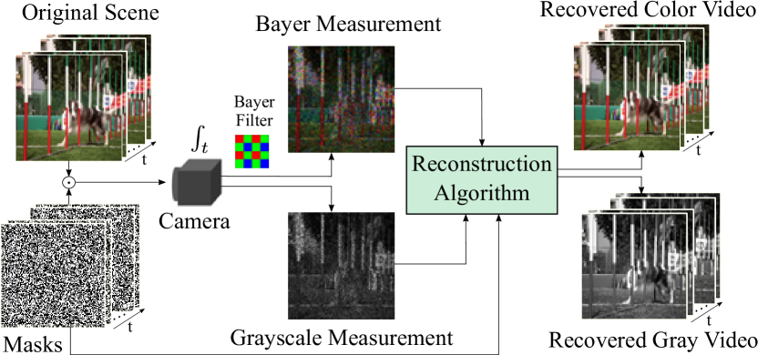
Figure 1: Schematic diagram of grayscale and color video SCI. A series of original frames are modulated through different masks, and then a camera is used to integrate encoded frames to obtain the compressed measurement, which is convenient for storage and transmission. Then, the measurement and masks are input into the reconstruction algorithm to recover the original video frames [5].

1.1 Video Snapshot Compressive Imaging

Traditional high-speed camera method for capturing high-speed scenes often faces the disadvantages of high hardware cost, high storage requirement and high transmission bandwidth. Bearing these challenges, video SCI system provides an elegant solution. As shown in Fig. 1, video SCI is an integrated hardware plus software system. For the hardware part (encoder), each frame of the original video is encoded by different masks, then a series of encoded frames is integrated (summed) by the (grayscale or color) camera to generate a compressed measurement. In this manner, video SCI can achieve efficient compression during optical domain imaging and improve the efficiency of video storage and transmission. At present, a variety of video SCI systems [4, 6, 7, 8, 9] have been built. The mask is usually generated by a digital micromirror device (DMD) or a spatial light modulator (SLM), and the encoded measurement is usually captured by a charge-coupled device (CCD) or a complementary metal-oxide semiconductor (CMOS) camera. In addition, for color video SCI [5], there is usually a Bayer-filter before the sensor array to capture different color components such as red, green or blue at different pixels, and ultimately the camera outputs the modulated Bayer measurement. For the software part (decoder), measurement and masks are usually fed into the reconstruction algorithm to recover the desired high-speed video.

1.2 Reconstruction Algorithms for Video SCI

In the decoding stage, the video SCI reconstruction algorithm aims to solve an ill-posed inverse problem. Traditional model-based reconstruction algorithms combines the idea of iterative optimization, such as generalized alternating projection (GAP) [10] and alternating direction method of multipliers (ADMM) [11], with a variety of prior knowledge, such as total variation (TV) [12], non-local low rank [13] and Gaussian mixture model [14]. Although these methods do not require any data to train the model, they usually suffer from poor reconstruction quality and long reconstruction time. In recent years, due to the development of deep learning and its strong generalization ability, researchers have constructed many learning-based models. For example, BIRNAT [15] uses convolutional neural networks (CNNs) and bidirectional recurrent neural networks (RNNs) for frame-by-frame reconstruction, while U-net [8] uses a simple U-shaped structure for fast reconstruction. RevSCI [16] can save training memory by using reversible mechanism [17]. Plug-and-play (PnP) methods, such as PnP-FFDNet [18] and PnP-FastDVDnet [19], make the model more flexible by integrating the deep denoising model into an iterative optimization algorithm. GAP-net [20], DUN-3DUnet [21] and Two-stage [22] further improve reconstruction quality and speed by using the ideas of deep unfolding [23]. Although previous methods have made great strides in video SCI reconstruction, at present, video SCI reconstruction still suffers from several key challenges:

• Since the video SCI sampling process compresses the entire temporal domain, it is important to establish long-term temporal correlation in the temporal domain during reconstruction. However, existing networks [24] use convolution to explore temporal correlation, and its receptive field are too small to be suitable for long-term temporal correlation extraction, resulting in poor reconstruction quality in complex high-speed scenes.

• Most existing end-to-end deep learning methods can not adapt to masks and input sizes changes. More specifically, the model usually needs to be retrained or fine-tuned when masks and input sizes change [25].

• PnP methods usually suffer from excessive smoothing and loss of local details.

Bearing these concerns in mind, we leverage the powerful model capacity of Transformer [26] and its ability to explore long-term dependencies to build an efficient video SCI reconstruction network.

1.3 Contributions of This Paper

In this paper, we propose a simple yet effective network for video SCI reconstruction. Our main contributions are as follows:

• We build an end-to-end deep video SCI reconstruction network based on spatial-temporal Transformer, which can be well applied to multiple video SCI reconstruction tasks.

• Through space-time factorization and local self-attention mechanism, we propose an efficient and flexible Transformer module, dubbed STFormer, with linear complexity, which can explore spatial-temporal correlations efficiently.

• We propose a Grouping Resnet Feed Forward module to further improve reconstruction quality by fusing multi-layer information and strengthening the correlation between different layers.

• We use multiple 3D convolutions to construct a token generation block to prevent loss of local details.

• Experimental results on a large number of simulated and real datasets demonstrate that our proposed algorithm achieves state-of-the-art (SOTA) results with better real-time performance compared to previous methods.

The rest of this paper is organized as follows: Sec. 2 introduces the mathematical model of grayscale and color video SCI and the related work of vision Transformers. In Sec. 3, we propose a reconstruction model STFormer for different video SCI reconstruction tasks, including grayscale video, color video and large-scale video. Sec. 4 shows experimental results on multiple simulated and real datasets. Sec. 5 concludes the entire paper.

2 Related Work

Since video SCI is an integrated system of hardware and software, in the following, we first introduce the mathematical model of video SCI , and then briefly review the related work of vision Transformer, which is the main part of the reconstruction network.

2.1 Review of Mathematical Model for video SCI

Video SCI system encodes high-dimensional video data into a 2D measurement, and coded aperture compressive temporal imaging (CACTI) [4] is one of the earliest video SCI systems. As shown in Fig. 1, the three-dimensional video data is first modulated by multiple masks. Then, the encoded high-speed scene is captured by a two-dimensional camera sensor through integration across the time dimension.

For grayscale video SCI system, let ${\bf X}\in\mathbb{R}^{n_{x}\times{n_{y}}\times{B}}$ denote the $B$-frame (grayscale) video data to be captured, ${{\bf M}}\in\mathbb{R}^{n_{x}\times{n_{y}}\times{B}}$ denote pre-defined masks. For each frame within the video $f=1,\ldots,B$, it is modulated by a mask in the image plane conducted by a 4-f system, and we can express this modulation as

$${\bf X}^{{}^{\prime}}(:,:,f)={\bf X}(:,:,f)\odot{{\bf M}}(:,:,f),$$ (1)

where ${\bf X}^{{}^{\prime}}\in\mathbb{R}^{n_{x}\times{n_{y}}\times{B}}$ denotes the modulated video data, ${\bf X}(:,:,f)$ denotes the $f$-th frame of the 3D video data ${\bf X}$, ${{\bf M}}(:,:,f)$ denotes the $f$-th mask of the 3D mask ${{\bf M}}$, and $\odot$ denotes the element-wise multiplication.

After this, by compressing across the time domain, the camera sensor plane captures a 2D compressed measurement ${{\bf Y}}\in\mathbb{R}^{n_{x}\times{n_{y}}}$, which can be expressed as

$${{\bf Y}}=\sum_{f=1}^{B}{{\bf X}^{{}^{\prime}}(:,:,f)+{\bf Z}},$$ (2)

where ${\bf Z}\in\mathbb{R}^{n_{x}\times{n_{y}}}$ denotes the measurement noise.

To keep the notations simple, we further give the vectorized formulation expression of Eq. (2). Firstly, we define $\operatorname{vec}(\cdot)$ as a vectorization operation of ensued matrix. Then we vectorize

$$\boldsymbol{y} = \operatorname{vec}({{\bf Y}})\in\mathbb{R}^{n_{x}{n_{y}}},$$ (3)

$$\boldsymbol{z} = \operatorname{vec}({\bf Z})\in\mathbb{R}^{n_{x}{n_{y}}},$$ (4)

$$\boldsymbol{x} = \left[\boldsymbol{x}_{1}^{\top},\ldots,\boldsymbol{x}^{\top}_{B}\right]^{\top}\in\mathbb{R}^{n_{x}{n_{y}{B}}},$$ (5)

where $\boldsymbol{x}_{f}=\operatorname{vec}({\bf X}(:,:,f))$. In addition, we define sensing matrix generated by masks in SCI system as

$${{\bf H}}=\left[{\bf D}_{1},\ldots,{\bf D}_{B}\right]\in\mathbb{R}^{n_{x}{n_{y}}\times{n_{x}{n_{y}{B}}}},$$ (6)

where ${\bf D}_{f}=\operatorname{Diag}(\operatorname{vec}({{\bf M}}_{f}))\in\mathbb{R}^{n_{x}n_{y}\times n_{x}n_{y}}$ is a diagonal matrix and its diagonal elements is filled by $\operatorname{vec}({{\bf M}}_{f})$, Finally, the vectorization expression of Eq. (2) is

$$\boldsymbol{y}={{\bf H}}{\boldsymbol{x}}+\boldsymbol{z}.$$ (7)

After obtaining the measurement $\boldsymbol{y}$ (captured by the camera), the next task is to develop a decoding algorithm, i.e., given $\boldsymbol{y}$ and ${{\bf H}}$, solve $\boldsymbol{x}$.

For color video SCI system, we use the Bayer pattern filter sensor, where each pixel captures only the red (R), green (G) or blue (B) channel of the raw data in a spatial layout such as ‘RGGB’. Since the colors of adjacent pixels are discontinuous, we divide the original measurement ${{\bf Y}}$ into four sub-measurements $\{{{\bf Y}}^{r},{{\bf Y}}^{g1},{{\bf Y}}^{g2},{{\bf Y}}^{b}\}\in\mathbb{R}^{\frac{n_{x}}{2}\times{\frac{n_{y}}{2}}}$. Correspondingly, the original masks ${{\bf M}}$ and original video frames ${\bf X}$ can also be divided into $\{{{\bf M}}^{r},{{\bf M}}^{g1},{{\bf M}}^{g2},{{\bf M}}^{b}\}\in\mathbb{R}^{\frac{n_{x}}{2}\times{\frac{n_{y}}{2}}\times{B}}$ and $\{{\bf X}^{r},{\bf X}^{g1},{\bf X}^{g2},{\bf X}^{b}\}\in\mathbb{R}^{\frac{n_{x}}{2}\times{\frac{n_{y}}{2}}\times{B}}$, respectively. The forward model of each channel can be expressed as

$${{\bf Y}}^{r} = \sum_{f=1}^{B}{{\bf X}^{r}_{f}\odot{{\bf M}}^{r}_{f}+{\bf Z}^{r}},$$ (8)

$${{\bf Y}}^{g1} = \sum_{f=1}^{B}{{\bf X}^{g1}_{f}\odot{{\bf M}}^{g1}_{f}+{\bf Z}^{g1}},$$ (9)

$${{\bf Y}}^{g2} = \sum_{f=1}^{B}{{\bf X}^{g2}_{f}\odot{{\bf M}}^{g2}_{f}+{\bf Z}^{g2}},$$ (10)

$${{\bf Y}}^{b} = \sum_{f=1}^{B}{{\bf X}^{b}_{f}\odot{{\bf M}}^{b}_{f}+{\bf Z}^{b}}.$$ (11)

For reconstruction, most previous algorithms [5, 18] reconstruct each sub-measurement separately, and then use off-the-shelf demosaic algorithms to obtain the desired RGB color videos. This channel-separated reconstruction algorithm cannot make good use of the correlation between channels and is inefficient. Therefore, we input all sub-measurements into our proposed reconstruction network simultaneously, and the reconstruction network directly outputs the desired RGB color video without employing previous demosaic algorithms.

2.2 Vision Transformers

Compared with convolutional networks [27, 28, 29], Vision Transformer (ViT) [30] and its variants [31, 32, 33, 34, 35] have achieved competitive results in the field of image classification [36]. However, the original ViT model training requires a large dataset (e.g., JFT-300M [37]) to achieve good results, DeiT [38] introduced some training strategies to enable the ViT model to achieve better performance in the ImageNet-1K dataset [36], but it still used the global self-attention mechanism, and the computational complexity increases quadratically with the image size. These greatly limit the application of ViT to dense prediction tasks such as object detection [39], semantic segmentation [40, 41, 42], and low-level tasks such as image denoising [43] and image restoration [44].

Moreover, PVT V2 [45] proposed a linear spatial reduction attention (SRA) layer, which uses average pooling to reduce spatial dimension, and achieve improvements on fundamental vision tasks such as classification, detection, and segmentation. MST [46] proposed a spectral-wise multi-head self-attention (S-MSA) and customized a mask-guided mechanism (MM), which effectively explores the application of Transformer to the spectral SCI task [47]. Swin Transformer [48] limits the self-attention calculation to the local window through the division of non-overlapping local windows and shifted window mechanism, which reduces the computational complexity of the Transformer to a linear relationship with the image size. However, Swin Transformer can only explore spatial correlation. Video Swin Transformer [49] can obtain local-scale temporal correlation by extending the local window to the temporal domain, but still cannot achieve good results in long-term correlation scenarios. TimeSformer [50] investigates the spatial-temporal correlation between tokens through a space-time factorization mechanism, and has achieved extremely competitive results in the field of video recognition. However, due to the use of global self-attention mechanism in the spatial domain, the computational complexity grows quadratically with the image size, and its positional embedding size is fixed, lacking the flexibility to change with input size. In addition, most of the existing Transformers [51, 52, 53] divide images or videos into non-overlapping patches to generate tokens, resulting in loss of local details and cannot be well applied to video reconstruction tasks in this work.

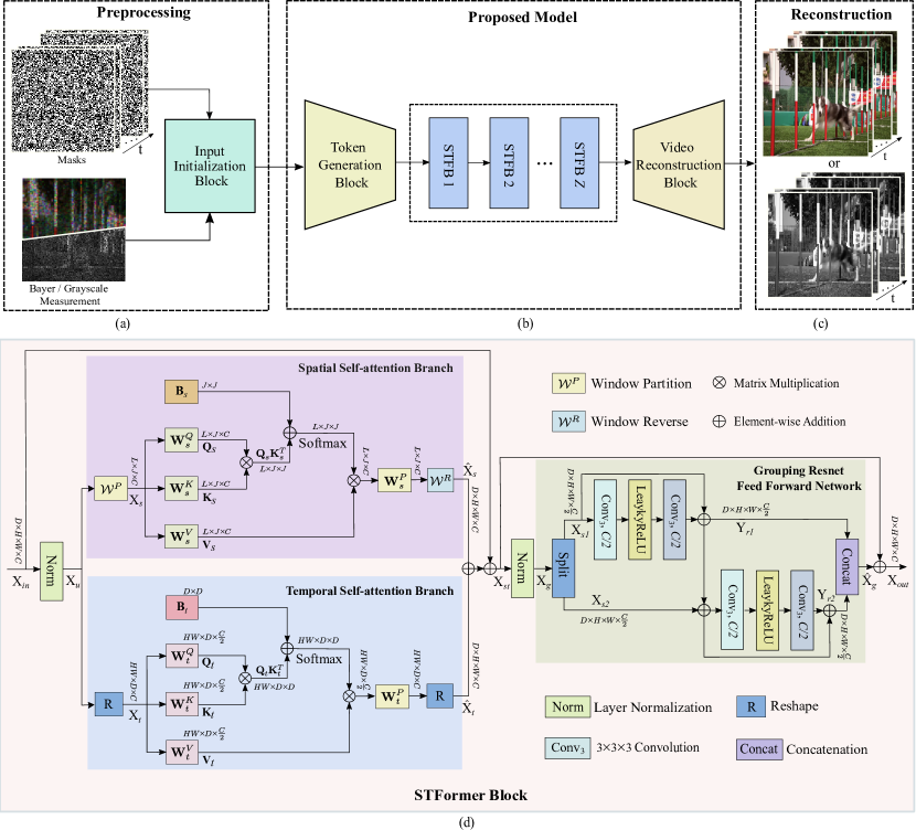
Figure 2: Architecture of the proposed STFormer and the overall process of color or grayscale video reconstruction. (a) After obtaining measurement and masks, the preprocessing stage generates the estimated value of the modulated frames through an input initialization block, and uses the estimated value as the input to the STFormer network for reconstruction. (b) The proposed STFormer network is composed of a token generation block, $Z$ STFormer blocks, and a video reconstruction block. (c) Reconstructed color or grayscale video. (d) Details of STFormer block, mainly composed of spatial self-attention branch, temporal self-attention branch and grouping resnet feed forward network, where $J=G_{h}{G_{w}}$ represents the number of tokens in each local window, $L=D\frac{HW}{J}$ represents the number of local windows, and $G_{h}$, $G_{w}$ represent the height and width of the local window, respectively. For the convenience of presentation, only the heads $N=1$ scenario is described here. Please refer to Sec. 3.2 for details.

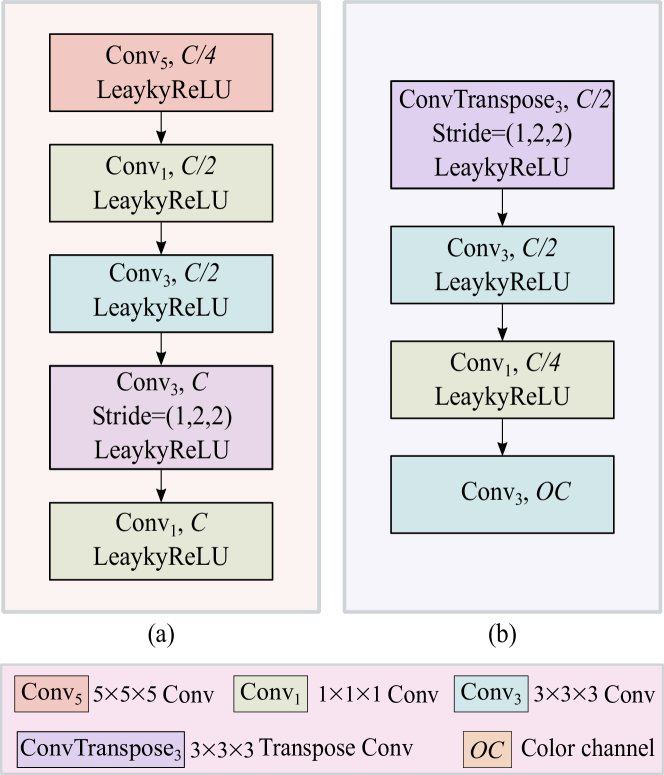
Figure 3: (a) Token generation block. (b) Video reconstruction block.

3 Proposed STFormer Network for Video SCI

Inspired by recent advances in Transformers, especially variants for video processing tasks, in this section, we introduce our proposed spatial-temporal Transformer in detail, which can efficiently explore long-range spatial-temporal correlations and lead to SOTA results on video SCI tasks.

3.1 Overall Architecture

The overall video reconstruction network architecture is depicted in Fig. 2. In the preprocessing stage shown in Fig. 2(a), we design the input initialization block with reference to GAP-net [20] and Two-stage [22]. By pre-processing masks (${{\bf M}}$) and measurement (${{\bf Y}}$) with the input initialization block, we can get a coarse estimation of the modulated frames $\hat{{\bf X}}\in\mathbb{R}^{n_{x}\times{n_{y}}\times{IC}\times{B}}$, where $IC=1$ represents the input channel number. Then, $\hat{{\bf X}}$ is fed into the token generation (TG) block [16] to get a series of consecutive tokens. We show in the supplementary material the implementation details of the pre-processing for grayscale and color video SCI in the input initialization block.

As demonstrated in Fig. 3(a), the TG block consists of five 3D convolutional layers, each followed by a LeakyReLU activation function [54]. Through the stride step and feature mapping in the convolutional layer, the number of finally generated tokens is $\frac{n_{x}}{2}\times\frac{n_{y}}{2}\times{B}$, and the feature dimension of each token is $C$. Different from most token generation methods, our proposed approach does not divide $\hat{{\bf X}}$ into non-overlapping patches, but uses 3D convolution for feature mapping, and then treats each point of the feature map as a token. This is beneficial to reduce the phenomenon of local detail loss.

To better explore the spatial-temporal correlation between each token, we design STFormer block (described in Section 3.2), and stack $Z$ STFormer blocks. It is worth noting that we do not use any downsampling method in each STFormer block, and the input and output dimensions of each STFormer block are kept consistent, which is also beneficial to prevent the loss of local details.

After the original tokens been mapped by $Z$ STFormer blocks, the spatial-temporal correlation between tokens has been well established. We input the tokens into the video reconstruction (VR) block [16] as shown in Fig. 3(b) to obtain the final desired video frames. In the VR block, the output channels number $OC$ of the last layer of convolution varies according to the reconstruction task, which is 1 for grayscale video reconstruction, and 3 for color video reconstruction.

3.2 STFormer Block

As shown in Fig. 2 (d), the STFormer block is composed of three parts: spatial self-attention (SSA) branch, temporal self-attenion (TSA) branch, and grouping resnet feed forward (GRFF) network. Among them, the SSA block can well explore the spatial correlation between tokens, and TSA block can well establish the temporal correlation between tokens, respectively. GRFF network can further investigate the correlation between adjacent tokens.

3.2.1 Spatial Self-attention Branch

Most of previous Transformer architectures used a global self-attention mechanism to calculate the correlation between tokens, which will cause the computational complexity of the Transformer model to increase quadratically with the number of tokens. This limits the application of Transformer to video SCI reconstruction tasks.

Bearing this in mind, in our proposed spatial self-attention branch, we use a local self-attention method to calculate the spatial correlation. As shown in Fig. 2 (d), in SSA branch, we first divide the feature map ${\bf X}_{u}\in\mathbb{R}^{D\times{H}\times{W}\times{C}}$ into a series of non-overlapping local windows ${\bf X}_{s}\in\mathbb{R}^{L\times{J}\times{C}}$, where $J=G_{h}{G_{w}}{G_{d}}$ represents the number of tokens in each local window, $L=D\frac{HW}{J}$ represents the number of local windows, and $G_{h},G_{w},G_{d}$ represent the height, width and timing length of the local window, respectively. Since spatial self-attention only calculates the spatial correlation between tokens, we set $G_{d}$ to 1, and the default values of $G_{h}$ and $G_{w}$ are 7. Then, the self-attention computation is restricted to each non-overlapping local window.

For the self-attention calculation of the local window, we first linearly map ${\bf X}_{s}$ to get $query\;{{\bf Q}}_{s}\in\mathbb{R}^{L\times{J}\times{C}}$, $key\;{{\bf K}}_{s}\in\mathbb{R}^{L\times{J}\times{C}}$ and $value\;{{\bf V}}_{s}\in\mathbb{R}^{L\times{J}\times{C}}$:

$${{\bf Q}}_{s} = {\bf X}_{s}{{\bf W}}^{Q}_{s},$$ (12)

$${{\bf K}}_{s} = {\bf X}_{s}{{\bf W}}^{K}_{s},$$ (13)

$${{\bf V}}_{s} = {\bf X}_{s}{{\bf W}}^{V}_{s},$$ (14)

where ${{\bf W}}^{Q}_{s}\in\mathbb{R}^{C\times{C}},{{\bf W}}^{K}_{s}\in\mathbb{R}^{C\times{C}}$ and ${{\bf W}}^{V}_{s}\in\mathbb{R}^{C\times{C}}$ represent projection matrices and share parameters between different windows. Then, we respectively divide ${{\bf Q}}_{s}$, ${{\bf K}}_{s}$, ${{\bf V}}_{s}$ into $N$ heads along the feature channel $C$:

$${{\bf Q}}_{s} = [{{\bf Q}}_{s}^{1},\cdots,{{\bf Q}}_{s}^{N}],$$ (15)

$${{\bf K}}_{s} = [{{\bf K}}_{s}^{1},\cdots,{{\bf K}}_{s}^{N}],$$ (16)

$${{\bf V}}_{s} = [{{\bf V}}_{s}^{1},\cdots,{{\bf V}}_{s}^{N}],$$ (17)

and the feature dimension of each head becomes $d_{h}=\frac{C}{N}$. For each head $i=1,\cdots,N$, the attention can be calculated by the local self-attention mechanism as:

$${\rm Attention}({{\bf Q}}_{s}^{i},{{\bf K}}_{s}^{i},{{\bf V}}_{s}^{i})={\rm SoftMax}({{\bf Q}}_{s}^{i}{{{\bf K}}_{s}^{i}}^{T}\sqrt{d}+{\bf B}_{s}^{i}){{\bf V}}_{s}^{i},$$ (18)

where ${{{\bf K}}_{s}^{i}}^{T}$ represents the transpose of matrix ${{\bf K}}_{s}^{i}$ and ${\bf B}_{s}^{i}\in\mathbb{R}^{J\times{J}}$ represents the learnable relative position encoding. After this, we concatenate the outputs of $N$ heads along the channel dimension and conduct a linear mapping to obtain the final output $\hat{{\bf X}}_{s}\in\mathbb{R}^{D\times{H}\times{W}\times{C}}$ of spatial local window multi-head self-attention mechanism ($SLW\mbox{-}MSA$):

$$\hat{{\bf X}}_{s}={\cal W}^{R}({{\bf W}}^{P}_{s}({\rm Concat}[{{\bf H}}_{s}^{1},\cdots,{{\bf H}}_{s}^{N}])),$$ (19)

where ${{\bf H}}_{s}^{i}={\rm Attention}({{\bf Q}}_{s}^{i},{{\bf K}}_{s}^{i},{{\bf V}}_{s}^{i})$, ${{\bf W}}_{s}^{P}\in\mathbb{R}^{C\times{C}}$ represents projection matrices and ${\cal W}^{R}$ represents window reverse returning to the original dimension. The whole process of the spatial self-attention branch can be expressed as:

$$\hat{{\bf X}}_{s}={\rm SLW\mbox{-}MSA}({\bf X}_{u}).$$ (20)

For the lack of connection between local windows, we refer to the shifted window partitioning approach of Swin Transformer [49] to establish the information interaction between local windows.

3.2.2 Temporal Self-attention Branch

Previous reconstruction algorithms typically use 2D or 3D convolutions to explore temporal correlations. Due to the local connection of convolutions, its receptive field is limited, which makes it incapable of investigating long-term correlation. Therefore, we exploit the long-term perception ability of Transformer to build a temporal self-attention branch. Different from the SSA branch, the TSA branch only performs self-attention on tokens in the same spatial position. In other words, the TSA branch does not calculate the spatial correlation between tokens.

As shown in Fig. 2(d), in TSA branch, for temporal self-attention calculation, we reshape the input ${\bf X}_{u}$ to ${\bf X}_{t}\in\mathbb{R}^{HW\times{D}\times{C}}$. After this, similar to the local window self-attention calculation of the SSA branch, we first linearly map ${\bf X}_{t}$ to get $query\;{{\bf Q}}_{t}\in\mathbb{R}^{HW\times{D}\times{\frac{C}{2}}}$, $key\;{{\bf K}}_{t}\in\mathbb{R}^{HW\times{D}\times{\frac{C}{2}}}$ and $value\;{{\bf V}}_{t}\in\mathbb{R}^{HW\times{D}\times{\frac{C}{2}}}$:

$${{\bf Q}}_{t}={\bf X}_{t}{{\bf W}}_{t}^{Q},{{\bf K}}_{t}={\bf X}_{t}{{\bf W}}_{t}^{K},{{\bf V}}_{t}={\bf X}_{t}{{\bf W}}_{t}^{V},$$ (21)

where ${{\bf W}}_{t}^{Q}\in\mathbb{R}^{C\times\frac{C}{2}},{{\bf W}}_{t}^{K}\in\mathbb{R}^{C\times{\frac{C}{2}}}$ and ${{\bf W}}_{t}^{V}\in\mathbb{R}^{C\times{\frac{C}{2}}}$ represent projection matrices and share parameters between different temporal windows.

Different from the SSA branch, we decrease the channel dimensions of ${{\bf Q}}_{t},{{\bf K}}_{t}$ and ${{\bf V}}_{t}$ to further reduce the computational complexity. Then, we respectively divide ${{\bf Q}}_{t}$, ${{\bf K}}_{t}$, ${{\bf V}}_{t}$ into $N$ heads along the feature channel: ${{\bf Q}}_{t}=[{{\bf Q}}_{t}^{1},\cdots,{{\bf Q}}_{t}^{N}]$, ${{\bf K}}_{t}=[{{\bf K}}_{t}^{1},\cdots,{{\bf K}}_{t}^{N}]$, ${{\bf V}}_{t}=[{{\bf V}}_{t}^{1},\cdots,{{\bf V}}_{t}^{N}]$, and the feature dimension of each head becomes $d_{h}=\frac{C}{2N}$. For each head $j=1,\cdots,N$, the attention can be calculated by the temporal window self-attention mechanism as:

$${\rm Attention}({{\bf Q}}_{t}^{j},{{\bf K}}_{t}^{j},{{\bf V}}_{t}^{j})={\rm SoftMax}({{\bf Q}}_{t}^{j}{{{\bf K}}_{t}^{j}}^{T}/\sqrt{d}+{\bf B}_{t}^{j}){{\bf V}}_{t}^{j},$$ (22)

where ${\bf B}_{t}^{j}\in\mathbb{R}^{D\times{D}}$ represents the learnable relative position encoding. Then, we concatenate the outputs of $N$ heads along the channel dimension and perform a linear mapping to obtain the final output $\hat{{\bf X}}_{t}\in\mathbb{R}^{D\times{H}\times{W}\times{C}}$ of temporal window multi-head self-attention mechanism ( $TW\mbox{-}MSA$):

$$\hat{{\bf X}}_{t}={{\bf R}}({{\bf W}}_{t}^{P}({\rm Concat}[{{\bf H}}_{t}^{1},\cdots,{{\bf H}}_{t}^{N}]))$$ (23)

where ${{\bf H}}_{t}^{j}={\rm Attention}({{\bf Q}}_{t}^{j},{{\bf K}}_{t}^{j},{{\bf V}}_{t}^{j})$, ${{\bf W}}_{t}^{P}\in\mathbb{R}^{\frac{C}{2}\times{C}}$ represents projection matrices, and ${{\bf R}}$ represents reshape operation. The whole process of the temporal self-attention branch can be expressed as:

$$\hat{{\bf X}}_{t}={\rm TW\mbox{-}MSA}({\bf X}_{u}).$$ (24)

3.2.3 Grouping Resnet Feed Forward Network

The FF network of a regular Transformer [26] uses two linear mapping layers to transform features; the first linear layer expands the channel dimension (usually by a factor of 4), and the second linear layer restores the channel dimension to the original one [55]. In the whole FF network process, the operation of each feature point are independent of each other, and there will be no interaction between feature points. In this work, we modify the original FF network with details shown in the GRFF network in Fig. 2(d). We divide the input feature map into two parts along the channel dimension; the first part of the feature is sent to a Resnet module, whose output is added to the second part of the feature, and the summed feature is used as input to another Resnet module. Following this, the outputs of the two Resnet modules are concatenated along the channel dimension to obtain the final output of the GRFF network. Given an input ${\bf X}_{g}\in\mathbb{R}^{D\times{H}\times{W}\times{C}}$, the whole GRFF network process can be expressed as:

$${\bf X}_{s1},{\bf X}_{s2} = {\rm Split}({\bf X}_{g}),$$ (25)

$${{\bf Y}}_{r1} = {\rm Resnet_{1}}({\bf X}_{s1}),$$ (26)

$${{\bf Y}}_{r2} = {\rm Resnet_{2}}({\bf X}_{s2}+{{\bf Y}}_{r1}),$$ (27)

$$\hat{{\bf X}}_{g} = {\rm Concat}([{{\bf Y}}_{r1},{{\bf Y}}_{r2}]),$$ (28)

where ${\rm Split}$ represents feature division along the channel, ${\rm Concat}$ represents feature merging across the channel dimension and $\hat{{\bf X}}_{g}\in\mathbb{R}^{D\times{H}\times{W}\times{C}}$ represents the output of the GRFF network. Overall, the GRFF network conducts more feature mapping by grouping and using the Resnet mechanism to achieve multi-layer information fusion, and the use of convolution enhances the information interaction between adjacent feature points. All of these are beneficial to improve the quality of video SCI reconstruction.

3.2.4 Whole Process of STFormer Block

In summary, the entire process of the STFormer block can be expressed as:

$${\bf X}_{u} = {\rm Norm}({\bf X}_{in}),$$ (29)

$$\hat{{\bf X}}_{s} = {\rm SLW\mbox{-}MSA}({\bf X}_{u}),$$ (30)

$$\hat{{\bf X}}_{t} = {\rm TW\mbox{-}MSA}({\bf X}_{u}),$$ (31)

$${\bf X}_{st} = {\bf X}_{in}+(\hat{{\bf X}}_{s}+\hat{{\bf X}}_{t}),$$ (32)

$$\hat{{\bf X}}_{g} = {\rm GRFF}({\rm Norm}({\bf X}_{st})),$$ (33)

$${\bf X}_{out} = {\bf X}_{st}+\hat{{\bf X}}_{g},$$ (34)

where ${\rm GRFF}(\cdot)$ represents the GRFF network processing, specifically described in Eq. (25)-(28), ${\rm Norm}(\cdot)$ represents the Layer Normalization [56], and ${\bf X}_{out}$ is the output of STFormer block.

3.2.5 Computational Complexity

In addition, we analyze the computational complexity of the spatial-temporal multi-head self-attention mechanism (${\rm ST\mbox{-}MSA}$), which consists of ${\rm SLW\mbox{-}MSA}$ and ${\rm TW\mbox{-}MSA}$:

$$\varOmega({\rm SLW\mbox{-}MSA}) =4HWDC^{2}+2G_{h}G_{w}HWDC,$$ (35)

$$\varOmega({\rm TW\mbox{-}MSA}) =2HWDC^{2}+HWD^{2}C,$$ (36)

$$\varOmega({\rm ST\mbox{-}MSA}) =\varOmega({\rm SLW\mbox{-}MSA})+\varOmega({\rm TW\mbox{-}MSA})$$ (37)

$$=6HWDC^{2}+2G_{h}G_{w}HWDC$$

$$\quad+HWD^{2}C,$$ (38)

where $\varOmega(\cdot)$ represents the computational complexity, $G_{h}$ and $G_{w}$ are generally set to 7, and $D$ is the number of frames, and compare it with the global multi-head self-attention mechanism (${\rm G\mbox{-}MSA}$) [46],

$$\varOmega({\rm G\mbox{-}MSA}) =4HWDC^{2}+2(HWD)^{2}C.$$ (39)

We can observe that the computational complexity of our proposed ${\rm ST\mbox{-}MSA}$ grows linearly with the spatial size $HW$, which is more computationally efficient than ${\rm G\mbox{-}MSA}$ (quadratic to $HW$).

TABLE I: The average PSNR in dB (left entry) and SSIM (right entry) and running time per measurement of different algorithms on 6 benchmark grayscale datasets. The best results are shown in bold and the second-best results are underlined.

Dataset	Kobe	Traffic	Runner	Drop	Crash	Aerial	Average	Running time(s)
GAP-TV[12]	26.46, 0.845	20.89, 0.715	28.52, 0.909	34.63, 0.970	24.82, 0.838	25.05, 0.828	26.73, 0.858	4.2 (CPU)
U-net[8]	27.79, 0.807	24.62, 0.840	34.12, 0.947	36.56, 0.949	26.43, 0.882	27.18, 0.869	29.45, 0.882	0.03 (GPU)
PnP-FFDNet[18]	30.50, 0.926	24.18, 0.828	32.15, 0.933	40.70, 0.989	25.42, 0.849	25.27, 0.829	29.70, 0.892	3.0 (GPU)
PnP-FastDVDnet[19]	32.73, 0.947	27.95, 0.932	36.29, 0.962	41.82, 0.989	27.32, 0.925	27.98, 0.897	32.35, 0.942	6.0 (GPU)
DeSCI[13]	33.25, 0.952	28.71, 0.925	38.48, 0.969	43.10, 0.993	27.04, 0.909	25.33, 0.860	32.65, 0.935	6180 (CPU)
BIRNAT[15]	32.71, 0.950	29.33, 0.942	38.70, 0.976	42.28, 0.992	27.84, 0.927	28.99, 0.917	33.31, 0.951	0.16 (GPU)
GAP-net-Unet-S12 [20]	32.09, 0.944	28.19, 0.929	38.12, 0.975	42.02, 0.992	27.83, 0.931	28.88, 0.914	32.86, 0.947	0.03 (GPU)
MetaSCI [25]	30.12, 0.907	26.95, 0.888	37.02, 0.967	40.61, 0.985	27.33, 0.906	28.31, 0.904	31.72, 0.926	0.03 (GPU)
RevSCI [16]	33.72, 0.957	30.02, 0.949	39.40, 0.977	42.93, 0.992	28.12, 0.937	29.35, 0.924	33.92, 0.956	0.19 (GPU)
DUN-3DUnet [21]	35.00, 0.969	31.76, 0.966	40.03, 0.980	44.96, 0.995	29.33, 0.956	30.46, 0.943	35.26, 0.968	1.35 (GPU)
STFormer-S	33.19, 0.955	29.19, 0.941	39.00, 0.979	42.84, 0.992	29.26, 0.950	30.13, 0.934	33.94, 0.958	0.14 (GPU)
STFormer-B	35.53, 0.973	32.15, 0.967	42.64, 0.988	45.08, 0.995	31.06, 0.970	31.56, 0.953	36.34, 0.974	0.49 (GPU)
STFormer-L	36.02, 0.975	32.74, 0.971	43.40, 0.989	45.48, 0.995	31.04, 0.971	31.85, 0.956	36.75, 0.976	0.92 (GPU)

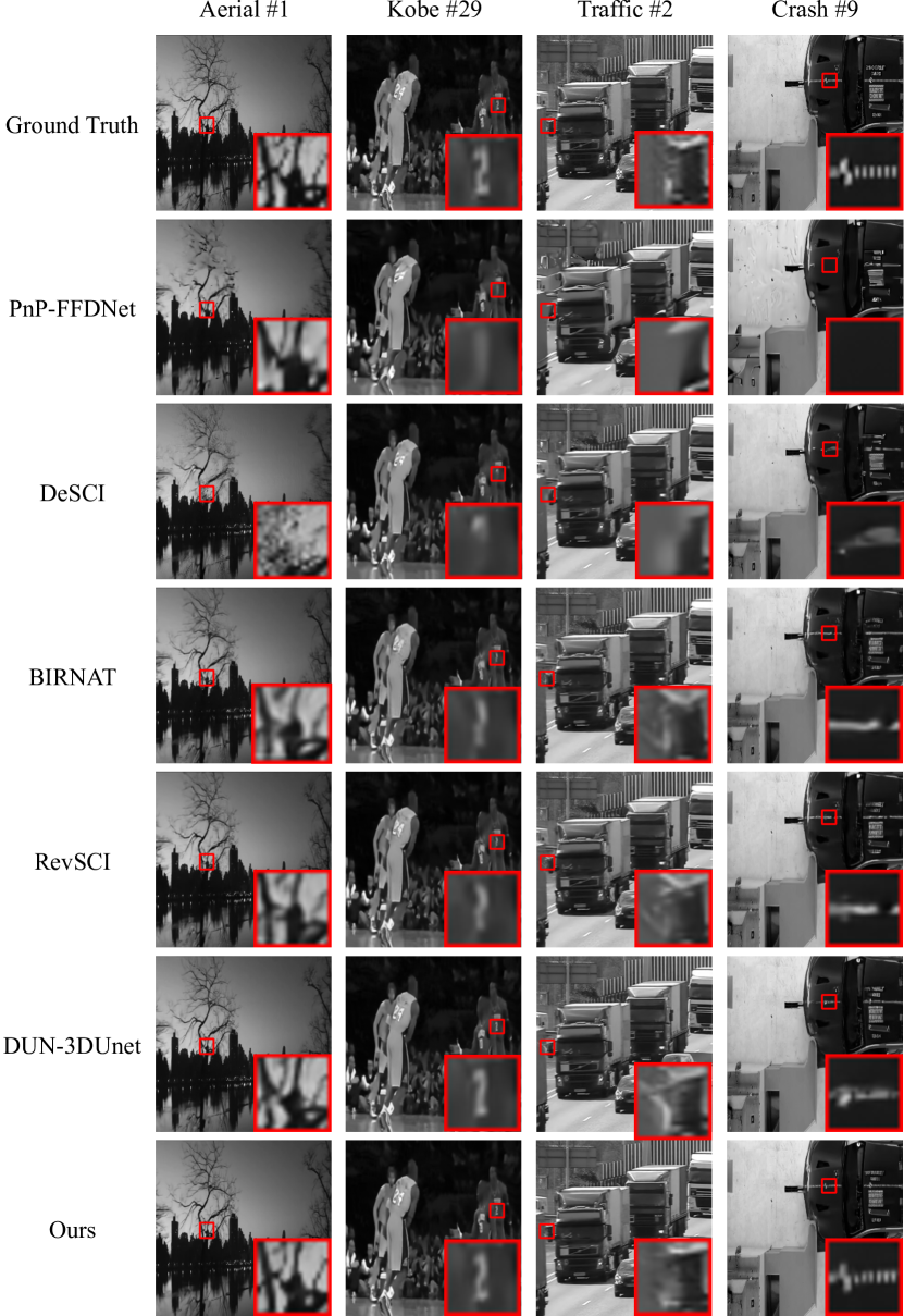
Figure 4: Comparison of reconstruction results of different reconstruction algorithms, PnP-FFDNet [18], DeSCI [13], BIRNAT [15], RevSCI [16], DUN-3DUnet [21], and our proposed STFormer-B on several benchmark grayscale video simulation datasets (Aerial, Kobe, Traffic, Crash). Zoom in for better view.

4 Experimental Results

In this section, we compare the performance of the proposed STFormer network with several SOTA video reconstruction methods on multiple simulation and real datasets. The peak-signal-to-noise-ratio (PSNR) and the structured similarity index metrics (SSIM) [57] are used to evaluate the performance of different video SCI reconstruction methods on simulation datasets.

4.1 Datasets

We use DAVIS2017 [58] as the training dataset for the model, which contains 90 different scenes with two resolutions: $480\times{894}$ and $1080\times{1920}$. For the grayscale simulation video testing datasets, we used six benchmark datasets including Kobe, Runner, Drop, Traffic , Aerial and Vehicle with a size of $256\times{256}\times{8}$, following the setup in [18]. For the color simulation video testing datasets, we follow PnP-FastDVDnet [19], using six benchmark color simulation datasets, including Beauty, Bosphorus,Jockey, Runner, ShakeNDry and Traffic with a size of $512\times{512}\times{3}\times{8}$. For the large-scale simulation video testing datasets, we used 4 benchmark large-scale simulation datasets, including Messi, Hummingbird, Swinger, Football used in [19].

For the real datasets, we used four datasets, including Duomino, Water Balloon, Hand and Hammer, captured by real video SCI cameras [8, 5] for grayscale and color video, respectively.

4.2 Implementation Details

During training, we perform data augmentation on DAVIS2017 using random horizontal flipping, random scaling, and random cropping. Following the CACTI imaging process, a series of measurements are generated. We use measurement and masks as inputs to train the STFormer network and use Adam optimizer [59] to optimize the model. Since our proposed STFormer network is flexible in input size, to speed up model training, we first train the model on data with a spatial resolution of $128\times{128}$ (100 epochs with an initial learning rate set be 0.0001) and then fine-tune it on data with a spatial resolution of $256\times{256}$ (20 epochs with an initial learning rate set be 0.00001). All experiments are run on PyTorch framework with 8 NVIDIA RTX 3090 GPUs.

4.3 Results on Simulation Datasets

In this section we present the results from the simulation to real dataset, first in grayscale and then in color.

To trade-off speed and performance, we have trained three models with different size, dubbed as STFormer-L, STFormer-B and STFormer-S, standing for Large, Base and Small networks respectively. The hyper-parameters of these models are as follows:

• STFormer-S: $C$=64, block numbers = {2,2,2,2},

• STFormer-B: $C$=256, block numbers = {2,2,2,2},

• STFormer-L: $C$=256, block numbers = {4,4,4,4},

where $C$ represents the number of input channels of the STFormer block. The model parameters (Params) and theoretical computational complexity (FLOPs) are shown in Tab. II, where we can observe that the parameters and computation of our proposed STFormer-S network are less than BIRNAT and RevSCI, and the STFormer-B network is less than DUN-3DUnet.

TABLE II: Computational complexity and average reconstruction quality of several SOTA algorithms on 6 grayscale benchmark datasets.

Method	Params (M)	FLOPs (G)	PSNR	SSIM
BIRNAT [15]	4.13	390.56	33.31	0.951
RevSCI [16]	5.66	766.95	33.92	0.956
DUN-3DUnet [21]	61.91	3975.83	35.26	0.968
STFormer-S	1.22	193.47	33.94	0.958
STFormer-B	19.48	3060.75	36.34	0.974
STFormer-L	36.81	5363.98	36.75	0.976

4.3.1 Grayscale Simulation Video

Currently, there are various methods for video SCI reconstruction, here we compare our method with some SOTA methods, $e.g.$, model-based iterative optimization methods (GAP-TV [12] and DeSCI [13]), end-to-end deep learning methods (U-net [8], MetaSCI [25], BIRNAT [15] and RevSCI [16]), plug-and-play methods (PnP-FFDNet [18], PnP-FastDVDnet [19]) and deep unfolding methods (GAP-net [20], DUN-3DUnet [21]). Tab. I presents the average PSNR and SSIM values for different reconstruction methods on 6 benchmark grayscale datasets and the average reconstruction time for a single measurement. Fig. 4 shows the visualization results of several SOTA reconstruction methods. We can observe that our proposed method achieves higher reconstruction quality and better real-time performance than previous SOTA methods by a large margin. From the visualization of reconstructed videos, our proposed method can recover more details and edge information. We summarize the observations in Tab. I and Fig. 4 as follows:

• Our proposed method (STFormer-L) achieves an average PSNR value of 36.75 dB and an SSIM value of 0.976. Compared with the previous SOTA method DUN-3DUnet (best published results) and the end-to-end deep learning method RevSCI, our proposed method achieves 1.49 dB and 2.83 dB higher average PSNR, respectively.

• For reconstruction running time, our proposed method achieves a good balance between reconstruction quality and running performance. The reconstruction quality of our proposed STFormer-B model is higher than 36 dB, and the running time is within 500ms. The running speed and reconstruction quality of the STFormer-S model are higher than most current reconstruction algorithms. Although U-net, MetaSCI, and GAP-net run faster, these algorithms have poor reconstruction quality, with an average PSNR value of less than 33 dB, which is more than 3 dB lower than STFormer-L. In some complex high-speed scenarios, such as Traffic, Crash, Aerial datasets, the reconstruction quality of these methods cannot even reach 29 dB.

• Benefit from the powerful model capacity of Transformer and its ability to effectively explore long-term dependencies, STFormer has excellent performance in complex scenarios (such as Aerial data), and high-speed scenarios (such as Crash data). The reconstruction quality of these two datasets reaches 31 dB for the first time. From the visualization frames in Fig. 4, we can recover clear edges of tree trunks in Aerial data and the marks on the vehicles in the Crash data. Previous SOTA methods are unable to reconstruct these details, which often leads to excessive smoothing.

TABLE III: Reconstruction quality of three different Transformers on 6 grayscale benchmark datasets showing average PSNR in dB and SSIM.

Dataset	TimeSformer [50]	Video Swin Transfomer [49]	STFormer-B
Kobe	31.12, 0.932	30.72, 0.924	35.53, 0.973
Traffic	27.50, 0.917	27.26, 0.911	32.15, 0.967
Runner	37.13, 0.974	37.25, 0.971	42.64, 0.988
Drop	40.14, 0.988	39.82, 0.987	45.08, 0.995
Crash	28.11, 0.931	28.46, 0.939	31.06, 0.970
Aerial	28.96, 0.915	29.07, 0.915	31.56, 0.953
Average	32.16, 0.943	32.09, 0.941	36.34, 0.974

To further explore the effectiveness of our proposed STFormer network for video SCI, we directly apply several SOTA video Transformer models, specifically TimeSformer [50] and Video Swin Transformer [49], to video SCI reconstruction tasks. For the original Video Swin Transformer, since the hierarchical structure makes the spatial resolution of the model output too low, we use U-net [60] to upsample the deep features and fuse them with the shallow features. In this way, the model can predict the final reconstruction result. As shown in Tab. III, the reconstruction quality of our proposed STFormer is significantly better than that of TimeSformer and Video Swin Transformer, which further verifies the effectiveness of the STFormer network for video SCI.

TABLE IV: The average PSNR in dB (left entry), SSIM (right entry) and running time per measurement of different algorithms on 6 benchmark color datasets. Best results are in bold and the second-best results are underlined.

Dataset	Beauty	Bosphorus	Jockey	Runner	ShakeNDry	Traffic	Average	Running time(s)
GAP-TV[12]	33.08, 0.964	29.70, 0.914	29.48, 0.887	29.10, 0.878	29.59, 0.893	19.84, 0.645	28.47, 0.864	10.80 (CPU)
DeSCI[13]	34.66, 0.971	32.88, 0.952	34.14, 0.938	36.16, 0.949	30.94, 0.905	24.62, 0.839	32.23, 0.926	92640 (CPU)
PnP-FFDNet-gray[18]	33.21, 0.963	28.43, 0.905	32.30, 0.918	30.83, 0.888	27.87, 0.861	21.03, 0.711	28.93, 0.874	13.20 (GPU)
PnP-FFDNet-color[18]	34.15, 0.967	33.06, 0.957	34.80, 0.943	35.32, 0.940	32.37, 0.940	24.55, 0.837	32.38, 0.931	97.80 (GPU)
PnP-FastDVDnet-gray[19]	33.01, 0.963	30.95, 0.934	33.51, 0.928	32.82, 0.900	29.92, 0.892	22.81, 0.776	30.50, 0.899	19.80 (GPU)
PnP-FastDVDnet-color [19]	35.27,0.972	37.24, 0.978	35.63,0.950	38.22, 0.965	33.71, 0.969	27.49, 0.915	34.60, 0.955	99.05 (GPU)
BIRNAT-color [61]	36.08, 0.975	38.30, 0.982	36.51, 0.956	39.65, 0.973	34.26, 0.951	28.03, 0.915	35.47, 0.959	0.98 (GPU)
STFormer-S	36.83, 0.980	38.36, 0.981	37.09, 0.963	40.56, 0.980	34.67, 0.952	29.00, 0.923	36.09, 0.963	0.54 (GPU)
STFormer-B	37.37, 0.981	40.39, 0.988	38.32, 0.968	42.45, 0.985	35.15, 0.956	30.24, 0.939	37.32, 0.970	1.95 (GPU)

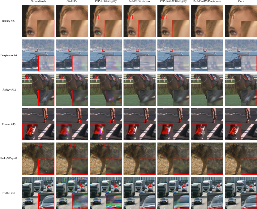
Figure 5: Comparison of reconstruction results of different reconstruction algorithms (GAP-TV [12], PnP-FFDNet-gray [18], PnP-FFDNet-color[18], PnP-FastDVD-gray [19], PnP-FastDVD-color[19], STFormer-B) on several benchmark color video simulation datasets (Beauty, Bosphorus, Jockey, Runner, ShakeNDry, Traffic). Zoom in for a better view.

4.3.2 Color Simulation Video

To verify the effectiveness of our method on various video SCI reconstruction tasks, we extend the STFormer network to the color SCI reconstruction task. We conduct related experiments on six benchmark color RGB datasets [19] with a spatial size of $512\times{512}\times{3}$, where $3$ represents the RGB channels. Similar to grayscale video, we compress the video with a compression rate of $B=8$. As shown in Fig. 1, we capture compressed Bayer measurements using a camera with a Bayer filter. For each dataset with 32 color video frames, we can get 4 Bayer measurements.

TABLE V: The average PSNR in dB (left entry) and SSIM (right entry) and running time per measurement of different algorithms on 4 benchmark large-scale datasets with a compression rate $B=8$. Best results are in bold.

Dataset	Messi	Hummingbird	Swinger	Football	Average	Running time(s)
GAP-TV[12]	25.20, 0.874	29.64, 0.897	24.64, 0.847	28.88, 0.919	27.09, 0.884	39.96 (CPU)
PnP-FFDNet[18]	30.83, 0.962	31.48, 0.945	25.27, 0.881	29.19, 0.930	29.19, 0.930	31.96 (GPU)
PnP-FastDVDnet[19]	31.57, 0.960	33.99, 0.878	26.30, 0.893	34.12, 0.965	31.50, 0.924	209.59 (GPU)
STFormer-S	33.55, 0.964	38.20, 0.965	31.98, 0.964	39.13, 0.988	35.72, 0.970	4.25 (GPU)

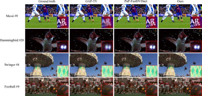
Figure 6: Comparison of reconstruction results of different reconstruction algorithms (GAP-TV [12], PnP-FFDNet [18], PnP-FastDVD[19], STFormer-S) on several benchmark large-scale video simulation datasets (Messi, Hummingbird, Swinger, Football). Zoom in for a better view.

Since STFormer is flexibility with respect to input size, in order to speed up training and save memory, we use the approach described in Sec. 4.2 to train the model on small-scale data. Considering the inflexibility of DUN-3DUnet [21] and RevSCI [16] for input size and masks, training a model with a spatial size of $512\times{512}$ requires a large amount of memory or training time. We only compare with iterative optimization algorithms (GAP-TV [12] and DeSCI [13]), end-to-end deep learning algorithm (BIRNAT-color [61]) and PnP algorithms (PnP-FFDNet [18], PnP-FastDVDnet [19]), it is worth noting that PnP methods are divided into gray version and color version according to the use of grayscale denoiser or color denoiser. The reconstruction results of different algorithms are shown in Fig. 5 and Tab. IV, we can summarize the observations as follows:

• The PSNR value of the STFormer network reaches 37.32 dB, which is 1.85 dB higher than the previous SOTA algorithm BIRNAT-color, especially in the high-speed motion scene Bosphorus, which is improved by 2.09 dB, and it exceeds 30 dB for the first time on the Traffic dataset. This shows that STFormer is also effective in color high-speed scenes.

• Regarding the running time of algorithm, the reconstruction of each measurement by the DeSCI algorithm is over 24 hours. Although the GAP-TV and PnP algorithms achieve higher real-time performance, they still take more than 10 seconds, while STFormer-B reconstruction algorithm only needs 1.95 seconds, which is more than 5 times faster than previous PnP methods. Recently, BIRNAT-color takes advantage of the end-to-end model to further improve the running speed of reconstruction. However, our proposed STFormer-S model achieves higher reconstruction quality and faster real-time performance.

• From the visualization results, our method can recover sharper edges of datasets Beauty, Jockey, Runner and Traffic, and can recover more local details of datasets Bosphorus, ShakeNDry. The reconstructed results of GAP-TV, PnP-FFDNet-gray and PnP-FastDVD-gray methods have some artifacts, while the reconstructed results of PnP-FFDNet-color and PnP-FastDVD-color methods have blurred edges and serious loss of details.

TABLE VI: Ablation study of STFormer on 6 grayscale benchmark datasets, the average PSNR in dB and SSIM is shown.

	TG Block	Video Swin Block	SSA Branch	TSA Branch	$MLP^{2}$	$MLP^{1}$	GRFF network	PSNR	SSIM
(a)		✓			✓			33.27	0.952
(b)	✓	✓			✓			34.41	0.961
(c)	✓	✓				✓		34.28	0.960
(d)	✓		✓		✓			33.41	0.954
(e)	✓		✓	✓	✓			35.26	0.969
(f)	✓		✓	✓		✓		35.15	0.967
(g)			✓	✓			✓	35.04	0.964
(h)	✓		✓	✓			✓	36.34	0.974

TABLE VII: Reconstruction quality and running time (s) on 6 grayscale benchmark datasets using STFormer with different number of channels and blocks

Model	Channel	Block	PSNR	SSIM	Running time(s)
STFormer-S	64	8	33.94	0.958	0.14
STFormer-B	256	8	36.34	0.974	0.49
STFormer-L	256	16	36.75	0.976	0.92

4.3.3 Large-scale Simulation Video

Similar to the benchmark color data, we further extend STFormer to large-scale datasets. Following [19], we used 4 benchmark large-scale datasets, including Messi, Hummingbird, Swinger with spatial size of $1080\times{1920}\times{3}$ and Football with the spatial size of $822\times{1920}\times{3}$, where $3$ represents RGB channels. Similar to the color simulation video, we generate measurements with a compression rate of $B=8$. Note that this is different from the various compression rates used in [19]. We set $B=8$ since we can use the same model trained for the mid-scale for the reconstruction of these large-scale datasets. This verifies the scalability and flexibility of our model. We can also train the model for large compression rates, only with additional training time and memory.

Due to the fact that network training of BIRNAT [15] and DUN-3DUnet [21] for large-scale datasets requires a lot of memory, while RevSCI [16] requires a longer training time, here we only compare STFormer with GAP-TV [12], PnP-FFDNet [18] and PnP-FastDVDnet [19]. Tab. V and Fig. 6 show the reconstruction results of these algorithms.

As shown in Fig. 6, we can observe that the results of GAP-TV reconstruction are blurry, PnP-FastDVDnet has some artifacts on some datasets, while our STFormer can achieve more realistic results. More importantly, our reconstruction on these datasets can reach more than 31 dB, which proves that video SCI can be applied to real scenes.

As for the running time, since we use a small version of STFormer, it can provide a more efficient runtime. As shown in Tab. V, for the reconstruction of a single measurement, our proposed algorithm takes only 4.25 seconds, which is 49 times faster than the previous SOTA algorithm PnP-FastDVDnet.

4.4 Ablation Study

To verify the effect of each module in the proposed STFormer network on the overall reconstruction quality, we conducted some ablation experiments on each module. Tab. VI shows the effect of each module on the reconstruction quality using the 6 grayscale benchmark datasets, where $\checkmark$ indicates that the reconstructed network includes this module, and no TG block indicates that the token generation method in the original Swin Transformer is used. In addition, $MLP^{2}$ and $MLP^{1}$ represent FF network expansion factors $\gamma=4$ and $\gamma=2$, respectively. We can get the following observations:

• Improvements in Token Generation Block: Tab. VI(g,h) show that our proposed TG block gain is 1.30 dB higher than its counterpart. Similarly, combining our TG block with other Transformer blocks can also greatly improve the reconstruction quality (see Tab. VI(a,b)).

• Improvements in STFormer Block: Here, we mainly compare the STFormer block with Video Swin Transformer block. Tab. VI(b,e) and Tab. VI(c,f) show that our proposed STFormer block can bring an improvement of at least 0.85 dB. In addition, we also verified the TSA branch of the STFormer block. As shown in Tab. VI(d,e), the reconstruction quality of the STFormer block with TSA branch can be improved by about 1.85 dB.

• Improvements in Grouping Resnet Feed Forward network: We compare the GRFF network with the traditional FF network consisting of MLP layers. As shown in Tab. VI(e,f,h), the GRFF network can provide an effective gain of more than 1.19 dB.

• Impact of width and depth of STFormer network: To verify the influence of the width and depth of the STFormer network on the reconstruction quality, we designed three models with different number of channels used to adjust the model width and number of blocks used to adjust the model depth. As shown in Tab. VII, increasing the width and depth of the model is beneficial to the improvement of the reconstruction quality, but it also leads to a longer running time.

TABLE VIII: Reconstruction quality on 6 grayscale benchmark datasets using random masks, the average PSNR in dB and SSIM are shown.

Mask	BIRNAT	RevSCI	DUN-3DUnet	STFormer-B
$Random\;Mask_{1}$	23.15, 0.731	18.90, 0.531	31.59, 0.934	36.28, 0.974
$Random\;Mask_{2}$	23.09, 0.730	18.99, 0.537	31.62, 0.934	36.33, 0.974
$Random\;Mask_{3}$	23.08, 0.728	18.96, 0.528	31.80, 0.935	36.32, 0.974

4.5 Flexibility

Previous end-to-end learning methods usually require retraining models for different masks and different spatial sizes. When dealing with large-scale data, they often require a large amount of memory and training time, which is inefficient. Transformer has a strong model capacity, and it can dynamically adjust the attention map according to different model inputs [44]. Along with our initialization method, the proposed STFormer network is robust to different masks.

To verify this flexibility, we randomly generate three masks that are not used during training. As shown in Tab. VIII, for different masks, the average PSNR value of the STFormer-B network reconstruction results remains within 0.06 dB, which is better than the current SOTA algorithms. By contrast, the previous end-to-end deep learning methods BIRNAT [15] and RevSCI [16] decrease more than 10 dB, and the deep unfolding DUN-3DUnet [21] decreases more than 3 dB.

Due to this flexibility of our proposed STFormer network, coupled with the use of STFormer block local window and relative position bias, the STFormer network trained on small-scale dataset can be used for large-scale datasets. As shown in Tab. IV and Tab. V, these STFormer models are trained on small-scale data (spatial size less than or equal to $256\times{256}$), and then directly used to reconstruct data with larger spatial size, all achieving SOTA reconstruction results.

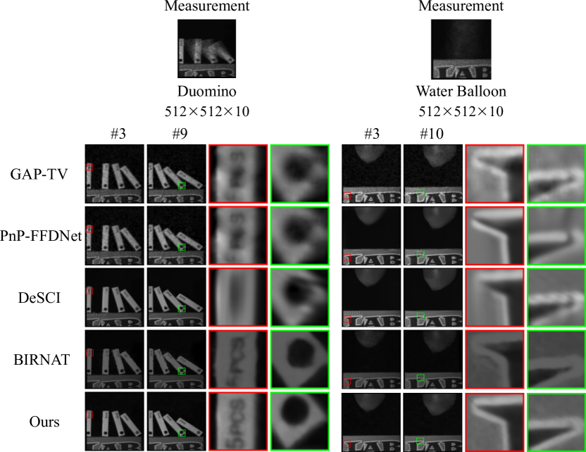
Figure 7: Comparison of reconstruction results of different reconstruction algorithms (GAP-TV [12], PnP-FFDNet [18], DeSCI [13], BIRNAT [15] STFormer-B) on several real datasets (Duomino, Water Ballon) with compression rate $B=10$. Zoom in for a better view.

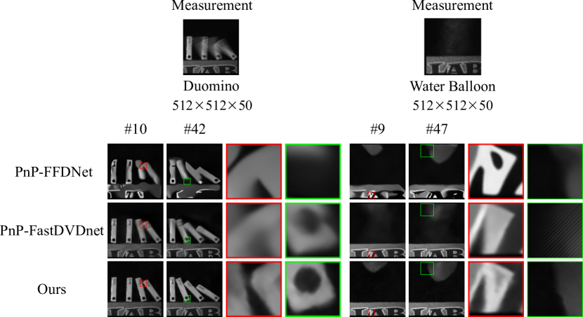
Figure 8: Comparison of reconstruction results of different reconstruction algorithms (PnP-FFDNet [18],PnP-FastDVDnet [19] STFormer-S) on several real datasets (Duomino, Water Ballon) with compression rate $B=50$. Zoom in for a better view.

4.6 Results on Real Video SCI Data

We validate our proposed method on grayscale and color real data. Since the real video SCI imaging system has uncertain noises, it is more challenging to reconstruct real data.

4.6.1 Grayscale Real Video

For the grayscale real data, we use Duomino, Water Ballon and Hand video data captured by [8]. It is worth noting that similar scenes are captured with different compression ratios, $i.e.,B=\{10,20,30,40,50\}$ and all snapshot measurements spatial size are $512\times{512}$. As shown in Fig 7, we first compared the reconstruction results with several SOTA reconstruction algorithms, namely GAP-TV [12], DeSCI [13], PnP-FFDNet [18] and BIRNAT [15] in the scenes of compression rate $B=10$. By zooming in on the local area, we can observe that our proposed algorithm can recover clear letters and sharp edges in the Dumino data and Water Ballon data, while the reconstruction results of GAP-TV, PnP-FFDNet, DeSCI and BIRNAT algorithms over-smooth these areas with some artifacts.

TABLE IX: Running time (seconds) of real data using different algorithms

Real Data	Pixel resolution	GAP-TV	DeSCI	PnP-FFDNet	PnP-FastDVDnet	STFormer-S
Hand10	$512\times{512}\times{10}$	37.8	2880.0	19.3	29.5	1.5
Hand20	$512\times{512}\times{20}$	88.7	4320.0	42.4	63.9	1.8
Hand30	$512\times{512}\times{30}$	163.0	6120.0	74.7	107.7	2.2
Hand50	$512\times{512}\times{50}$	303.4	12600.0	144.5	203.9	2.7

In addition, our proposed STFormer network can also achieve good reconstruction results at high compression rates, e.g., at $B=50$, which further verifies the capability of our method to explore long-term temporal dependencies. Although previous reconstruction algorithms can reconstruct high-compression data, their reconstruction results are too smooth and require a long running time (See Tab. IX); in particular, PnP-FastDVDnet takes 3.4 minutes, DeSCI algorithm reconstruction time is more than 3 hours and and our method only needs 2.7 seconds. Fig. 10 and Fig. 11 show the reconstruction results of Hand and Duomino with $B=10,20,30,50$, respectively. We can observe that our proposed method can well reconstruct the desired high-speed video frames with compression rates from 10 to 50. Compare with previous SOTA method PnP-FastDVDnet, our results can provide clear details of Duomino and the Water Balloon even at $B=50$. Please refer to Fig. 8.

We have further verified our proposed algorithms on the new video SCI system built at Westlake University similar to [8] but with different masks and different compression rates. Please refer to the reconstructed videos in the supplemental material.

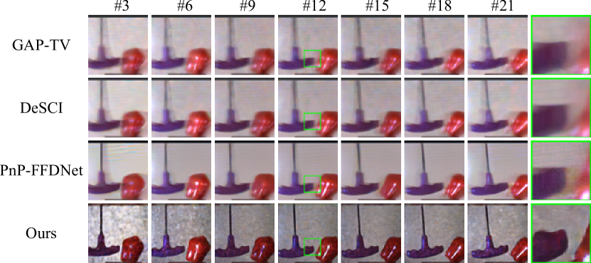
Figure 9: Comparison of reconstruction results of different reconstruction algorithms (GAP-TV [12], DeSCI [13], PnP-FFDNet [18] and STFormer-S) on real color data (Hammer). Zoom in for a better view.

4.6.2 Color Real Video

For the color real data, we use Hammer video data captured by [5]. The spatial resolution of a single Bayer mosaic measurement is $512\times{512}$ and the compression rate $B$ is 22. Since most reconstruction algorithms cannot be applied to the color data, we only compare our method with GAP-TV [12], DeSCI [13] and PnP-FFDNet [18]. Fig. 9 shows the reconstruction results of these algorithms. By zooming in on the local areas, we can see that the reconstruction results of GAP-TV, DeSCI, and PnP-FFDNet methods have some artifacts and blurred edges, but our proposed STFormer method can restore these sharpe edges.

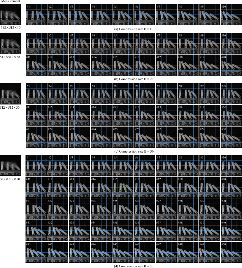
Figure 10: Reconstructed real video data (Duomino) with compression rate $B$ from 10 to 50, Mesh is added to better visualize motion details. The reconstruction algorithm is STFormer-S.

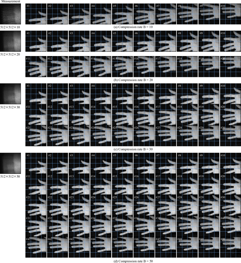
Figure 11: Reconstructed real video data (Hand) with compression rate $B$ from 10 to 50, Mesh is added to better visualize motion details. The reconstruction model is STFormer-S.

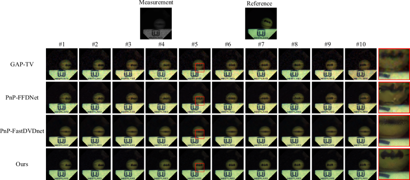
Figure 12: Comparison of reconstruction results of different reconstruction algorithms (GAP-TV [12], PnP-FFDNet [18],PnP-FastDVDnet [19] and STFormer-B) on real color data (Ball Rotate). Zoom in for a better view.

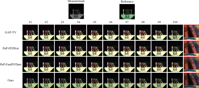
Figure 13: Comparison of reconstruction results of different reconstruction algorithms (GAP-TV [12], PnP-FFDNet [18],PnP-FastDVDnet [19] and STFormer-B) on real color data (Duomino). Zoom in for a better view.

Furthermore, to fill the gap of lacking real color data for video SCI, we have built a new video SCI system at Westlake University using RGB sensors but with different masks and different compression rates. The reconstructed videos are shown in Fig. 12 and Fig. 13. Comparing with previous SOTA algorithms, the reconstruction results of our proposed STFormer network are closer to the real color and can recover more details. Please refer to the enlarged areas in Figs. 12-13.

5 Conclusions

In this paper, we present STFormer, a spatial-temporal Transformer, to conduct the reconstruction task of video snapshot compressive imaging. Our proposed STFormer network consists of token generation block, video reconstruction block and a series of STFormer blocks. In particular, each STFormer block restricts the self-attention calculation to the spatial local window and time domain through the space-time factorization and local self-attention mechanism, which improves the computational efficiency and increases the flexibility of the model for multi-scale input. Since STFormer can effectively explore spatial-temporal correlations, it achieves SOTA results on multiple video SCI reconstruction tasks. Especially for complex and high-speed motion scenes, STFormer can achieve a reconstruction quality of more than 30 dB, far exceeding the previous SOTA reconstruction algorithms. Furthermore, STFormer is the first end-to-end deep learning network with flexibility of masks and input scale, while enjoying fast inference, greatly facilitating applications of video SCI system in our daily life.

Although STFormer has achieved satisfactory results on video SCI, the current video SCI reconstruction still faces many difficulties, such as the research of deep learning models suitable for different compression rates. In addition, for the real color data, due to the existence of complicated noise, there is still a huge gap between the reconstruction results and the real scene.

Regarding future work plans, one is to extend our STFormer network to other SCI reconstruction tasks, such as spectral SCI [62, 63, 64, 65], and the other is to use STFormer as a backbone for video action recognition [66], video object tracking [67] and other tasks [68].

References

- [1] J. N. Mait, G. W. Euliss, and R. A. Athale, “Computational imaging,” Adv. Opt. Photon., vol. 10, no. 2, pp. 409–483, Jun 2018.
- [2] Y. Altmann, S. McLaughlin, M. J. Padgett, V. K. Goyal, A. O. Hero, and D. Faccio, “Quantum-inspired computational imaging,” Science, vol. 361, no. 6403, p. eaat2298, 2018.
- [3] X. Yuan, D. J. Brady, and A. K. Katsaggelos, “Snapshot compressive imaging: Theory, algorithms, and applications,” IEEE Signal Processing Magazine, vol. 38, no. 2, pp. 65–88, 2021.
- [4] P. Llull, X. Liao, X. Yuan, J. Yang, D. Kittle, L. Carin, G. Sapiro, and D. J. Brady, “Coded aperture compressive temporal imaging,” Optics express, vol. 21, no. 9, pp. 10 526–10 545, 2013.
- [5] X. Yuan, P. Llull, X. Liao, J. Yang, D. J. Brady, G. Sapiro, and L. Carin, “Low-cost compressive sensing for color video and depth,” in Proceedings of the IEEE Conference on Computer Vision and Pattern Recognition, 2014, pp. 3318–3325.
- [6] Y. Hitomi, J. Gu, M. Gupta, T. Mitsunaga, and S. K. Nayar, “Video from a single coded exposure photograph using a learned over-complete dictionary,” in 2011 International Conference on Computer Vision. IEEE, 2011, pp. 287–294.
- [7] D. Reddy, A. Veeraraghavan, and R. Chellappa, “P2C2: Programmable pixel compressive camera for high speed imaging,” in CVPR 2011. IEEE, 2011, pp. 329–336.
- [8] M. Qiao, Z. Meng, J. Ma, and X. Yuan, “Deep learning for video compressive sensing,” APL Photonics, vol. 5, no. 3, p. 30801, 2020.
- [9] Y. Sun, X. Yuan, and S. Pang, “Compressive high-speed stereo imaging,” Optics express, vol. 25, no. 15, pp. 18 182–18 190, 2017.
- [10] X. Liao, H. Li, and L. Carin, “Generalized alternating projection for weighted-2,1 minimization with applications to model-based compressive sensing,” SIAM Journal on Imaging Sciences, vol. 7, no. 2, pp. 797–823, 2014.
- [11] S. Boyd, N. Parikh, and E. Chu, Distributed optimization and statistical learning via the alternating direction method of multipliers. Now Publishers Inc, 2011.
- [12] X. Yuan, “Generalized alternating projection based total variation minimization for compressive sensing,” in 2016 IEEE International Conference on Image Processing (ICIP). IEEE, 2016, pp. 2539–2543.
- [13] Y. Liu, X. Yuan, J. Suo, D. J. Brady, and Q. Dai, “Rank minimization for snapshot compressive imaging,” IEEE transactions on pattern analysis and machine intelligence, vol. 41, no. 12, pp. 2990–3006, 2018.
- [14] J. Yang, X. Liao, X. Yuan, P. Llull, D. J. Brady, G. Sapiro, and L. Carin, “Compressive sensing by learning a Gaussian mixture model from measurements,” IEEE Transactions on Image Processing, vol. 24, no. 1, pp. 106–119, 2014.
- [15] Z. Cheng, R. Lu, Z. Wang, H. Zhang, B. Chen, Z. Meng, and X. Yuan, “BIRNAT: Bidirectional recurrent neural networks with adversarial training for video snapshot compressive imaging,” in European Conference on Computer Vision. Springer, 2020, pp. 258–275.
- [16] Z. Cheng, B. Chen, G. Liu, H. Zhang, R. Lu, Z. Wang, and X. Yuan, “Memory-efficient network for large-scale video compressive sensing,” in Proceedings of the IEEE/CVF Conference on Computer Vision and Pattern Recognition, 2021, pp. 16 246–16 255.
- [17] J. Behrmann, W. Grathwohl, R. T. Chen, D. Duvenaud, and J.-H. Jacobsen, “Invertible residual networks,” in International Conference on Machine Learning. PMLR, 2019, pp. 573–582.
- [18] X. Yuan, Y. Liu, J. Suo, and Q. Dai, “Plug-and-play algorithms for large-scale snapshot compressive imaging,” in Proceedings of the IEEE/CVF Conference on Computer Vision and Pattern Recognition, 2020, pp. 1447–1457.
- [19] X. Yuan, Y. Liu, J. Suo, F. Durand, and Q. Dai, “Plug-and-play algorithms for video snapshot compressive imaging,” IEEE Transactions on Pattern Analysis Machine Intelligence, no. 01, pp. 1–1, 2021.
- [20] Z. Meng, S. Jalali, and X. Yuan, “Gap-net for snapshot compressive imaging,” arXiv preprint arXiv:2012.08364, 2020.
- [21] Z. Wu, J. Zhang, and C. Mou, “Dense deep unfolding network with 3D-CNN prior for snapshot compressive imaging,” in Proceedings of the IEEE/CVF International Conference on Computer Vision, 2021, pp. 4892–4901.
- [22] S. Zheng, X. Yang, and X. Yuan, “Two-stage is enough: A concise deep unfolding reconstruction network for flexible video compressive sensing,” arXiv preprint arXiv:2201.05810, 2022.
- [23] C. Yang, S. Zhang, and X. Yuan, “Ensemble learning priors unfolding for scalable snapshot compressive sensing,” in European Conference on Computer Vision. Springer, 2022.
- [24] W. Saideni, D. Helbert, F. Courreges, and J.-P. Cances, “An overview on deep learning techniques for video compressive sensing,” Applied Sciences, vol. 12, no. 5, p. 2734, 2022.
- [25] Z. Wang, H. Zhang, Z. Cheng, B. Chen, and X. Yuan, “MetaSCI: Scalable and adaptive reconstruction for video compressive sensing,” in Proceedings of the IEEE/CVF Conference on Computer Vision and Pattern Recognition, 2021, pp. 2083–2092.
- [26] A. Vaswani, N. Shazeer, N. Parmar, J. Uszkoreit, L. Jones, A. N. Gomez, Ł. Kaiser, and I. Polosukhin, “Attention is all you need,” in Advances in Neural Information Processing Systems, 2017, pp. 5998–6008.
- [27] A. Krizhevsky, I. Sutskever, and G. E. Hinton, “Imagenet classification with deep convolutional neural networks,” Advances in neural information processing systems, vol. 25, pp. 1097–1105, 2012.
- [28] K. He, X. Zhang, S. Ren, and J. Sun, “Deep residual learning for image recognition,” in Proceedings of the IEEE conference on computer vision and pattern recognition, 2016, pp. 770–778.
- [29] G. Huang, Z. Liu, L. Van Der Maaten, and K. Q. Weinberger, “Densely connected convolutional networks,” in Proceedings of the IEEE conference on computer vision and pattern recognition, 2017, pp. 4700–4708.
- [30] A. Dosovitskiy, L. Beyer, A. Kolesnikov, D. Weissenborn, X. Zhai, T. Unterthiner, M. Dehghani, M. Minderer, G. Heigold, S. Gelly et al., “An image is worth 16x16 words: Transformers for image recognition at scale,” in International Conference on Learning Representations, 2020.
- [31] X. Dong, J. Bao, D. Chen, W. Zhang, N. Yu, L. Yuan, D. Chen, and B. Guo, “Cswin transformer: A general vision transformer backbone with cross-shaped windows,” in Proceedings of the IEEE/CVF Conference on Computer Vision and Pattern Recognition, 2022, pp. 12 124–12 134.
- [32] X. Zhu, W. Su, L. Lu, B. Li, X. Wang, and J. Dai, “Deformable DETR: Deformable transformers for end-to-end object detection,” in International Conference on Learning Representations, 2020.
- [33] L. Yuan, Y. Chen, T. Wang, W. Yu, Y. Shi, Z.-H. Jiang, F. E. Tay, J. Feng, and S. Yan, “Tokens-to-token vit: Training vision transformers from scratch on imagenet,” in Proceedings of the IEEE/CVF International Conference on Computer Vision, 2021, pp. 558–567.
- [34] W. Wang, E. Xie, X. Li, D.-P. Fan, K. Song, D. Liang, T. Lu, P. Luo, and L. Shao, “Pyramid vision transformer: A versatile backbone for dense prediction without convolutions,” in Proceedings of the IEEE/CVF International Conference on Computer Vision, 2021, pp. 568–578.
- [35] K. Han, Y. Wang, H. Chen, X. Chen, J. Guo, Z. Liu, Y. Tang, A. Xiao, C. Xu, Y. Xu et al., “A survey on vision transformer,” IEEE Transactions on Pattern Analysis and Machine Intelligence, 2022.
- [36] J. Deng, W. Dong, R. Socher, L.-J. Li, K. Li, and L. Fei-Fei, “Imagenet: A large-scale hierarchical image database,” in 2009 IEEE conference on computer vision and pattern recognition. Ieee, 2009, pp. 248–255.
- [37] C. Sun, A. Shrivastava, S. Singh, and A. Gupta, “Revisiting unreasonable effectiveness of data in deep learning era,” in Proceedings of the IEEE international conference on computer vision, 2017, pp. 843–852.
- [38] H. Touvron, M. Cord, M. Douze, F. Massa, A. Sablayrolles, and H. Jégou, “Training data-efficient image transformers & distillation through attention,” in International Conference on Machine Learning. PMLR, 2021, pp. 10 347–10 357.
- [39] T.-Y. Lin, M. Maire, S. Belongie, J. Hays, P. Perona, D. Ramanan, P. Dollár, and C. L. Zitnick, “Microsoft COCO: Common objects in context,” in European conference on computer vision. Springer, 2014, pp. 740–755.
- [40] B. Zhou, H. Zhao, X. Puig, S. Fidler, A. Barriuso, and A. Torralba, “Scene parsing through ADE20K dataset,” in Proceedings of the IEEE conference on computer vision and pattern recognition, 2017, pp. 633–641.
- [41] B. Zhou, H. Zhao, X. Puig, T. Xiao, S. Fidler, A. Barriuso, and A. Torralba, “Semantic understanding of scenes through the ADE20K dataset,” International Journal of Computer Vision, vol. 127, no. 3, pp. 302–321, 2019.
- [42] Z. Huang, X. Wang, L. Huang, C. Huang, Y. Wei, and W. Liu, “Ccnet: Criss-cross attention for semantic segmentation,” in Proceedings of the IEEE/CVF International Conference on Computer Vision, 2019, pp. 603–612.
- [43] K. Zhang, W. Zuo, Y. Chen, D. Meng, and L. Zhang, “Beyond a gaussian denoiser: Residual learning of deep cnn for image denoising,” IEEE transactions on image processing, vol. 26, no. 7, pp. 3142–3155, 2017.
- [44] J. Liang, J. Cao, G. Sun, K. Zhang, L. Van Gool, and R. Timofte, “SwinIR: Image restoration using swin transformer,” in Proceedings of the IEEE/CVF International Conference on Computer Vision, 2021, pp. 1833–1844.
- [45] W. Wang, E. Xie, X. Li, D.-P. Fan, K. Song, D. Liang, T. Lu, P. Luo, and L. Shao, “Pvt v2: Improved baselines with pyramid vision transformer,” Computational Visual Media, pp. 1–10, 2022.
- [46] Y. Cai, J. Lin, X. Hu, H. Wang, X. Yuan, Y. Zhang, R. Timofte, and L. Van Gool, “Mask-guided spectral-wise transformer for efficient hyperspectral image reconstruction,” in Proceedings of the IEEE/CVF Conference on Computer Vision and Pattern Recognition, 2022, pp. 17 502–17 511.
- [47] Z. Meng, Z. Yu, K. Xu, and X. Yuan, “Self-supervised neural networks for spectral snapshot compressive imaging,” in Proceedings of the IEEE/CVF International Conference on Computer Vision, 2021, pp. 2622–2631.
- [48] Z. Liu, Y. Lin, Y. Cao, H. Hu, Y. Wei, Z. Zhang, S. Lin, and B. Guo, “Swin transformer: Hierarchical vision transformer using shifted windows,” in Proceedings of the IEEE/CVF International Conference on Computer Vision, 2021, pp. 10 012–10 022.
- [49] Z. Liu, J. Ning, Y. Cao, Y. Wei, Z. Zhang, S. Lin, and H. Hu, “Video swin transformer,” in Proceedings of the IEEE/CVF Conference on Computer Vision and Pattern Recognition, 2022, pp. 3202–3211.
- [50] G. Bertasius, H. Wang, and L. Torresani, “Is space-time attention all you need for video understanding?” in ICML, vol. 2, no. 3, 2021, p. 4.
- [51] R. Wang, D. Chen, Z. Wu, Y. Chen, X. Dai, M. Liu, Y.-G. Jiang, L. Zhou, and L. Yuan, “Bevt: Bert pretraining of video transformers,” in Proceedings of the IEEE/CVF Conference on Computer Vision and Pattern Recognition, 2022, pp. 14 733–14 743.
- [52] K. He, X. Chen, S. Xie, Y. Li, P. Dollár, and R. Girshick, “Masked autoencoders are scalable vision learners,” in Proceedings of the IEEE/CVF Conference on Computer Vision and Pattern Recognition, 2022, pp. 16 000–16 009.
- [53] H. Bao, L. Dong, and F. Wei, “Beit: Bert pre-training of image transformers,” arXiv preprint arXiv:2106.08254, 2021.
- [54] B. Xu, N. Wang, T. Chen, and M. Li, “Empirical evaluation of rectified activations in convolutional network,” arXiv preprint arXiv:1505.00853, 2015.
- [55] S. W. Zamir, A. Arora, S. Khan, M. Hayat, F. S. Khan, and M.-H. Yang, “Restormer: Efficient transformer for high-resolution image restoration,” in Proceedings of the IEEE/CVF Conference on Computer Vision and Pattern Recognition, 2022, pp. 5728–5739.
- [56] J. L. Ba, J. R. Kiros, and G. E. Hinton, “Layer normalization,” arXiv preprint arXiv:1607.06450, 2016.
- [57] Z. Wang, A. C. Bovik, H. R. Sheikh, and E. P. Simoncelli, “Image quality assessment: from error visibility to structural similarity,” IEEE transactions on image processing, vol. 13, no. 4, pp. 600–612, 2004.
- [58] J. Pont-Tuset, F. Perazzi, S. Caelles, P. Arbeláez, A. Sorkine-Hornung, and L. Van Gool, “The 2017 davis challenge on video object segmentation,” arXiv preprint arXiv:1704.00675, 2017.
- [59] D. P. Kingma and J. Ba, “Adam: A method for stochastic optimization,” arXiv preprint arXiv:1412.6980, 2014.
- [60] O. Ronneberger, P. Fischer, and T. Brox, “U-Net: Convolutional networks for biomedical image segmentation,” in International Conference on Medical image computing and computer-assisted intervention. Springer, 2015, pp. 234–241.
- [61] Z. Cheng, B. Chen, R. Lu, Z. Wang, H. Zhang, Z. Meng, and X. Yuan, “Recurrent neural networks for snapshot compressive imaging,” IEEE Transactions on Pattern Analysis and Machine Intelligence, 2022.
- [62] Z. Meng, J. Ma, and X. Yuan, “End-to-end low cost compressive spectral imaging with spatial-spectral self-attention,” in European Conference on Computer Vision. Springer, 2020, pp. 187–204.
- [63] L. Wang, Z. Wu, Y. Zhong, and X. Yuan, “Snapshot spectral compressive imaging reconstruction using convolution and contextual transformer,” Photonics Research, vol. 10, no. 8, pp. 1848–1858, 2022.
- [64] X. Yuan, T.-H. Tsai, R. Zhu, P. Llull, D. Brady, and L. Carin, “Compressive hyperspectral imaging with side information,” IEEE Journal of Selected Topics in Signal Processing, vol. 9, no. 6, pp. 964–976, September 2015.
- [65] X. Miao, X. Yuan, Y. Pu, and V. Athitsos, “lambda-net: Reconstruct hyperspectral images from a snapshot measurement,” in Proceedings of the IEEE/CVF International Conference on Computer Vision, 2019, pp. 4059–4069.
- [66] C.-Y. Wu, M. Zaheer, H. Hu, R. Manmatha, A. J. Smola, and P. Krähenbühl, “Compressed video action recognition,” in Proceedings of the IEEE conference on computer vision and pattern recognition, 2018, pp. 6026–6035.
- [67] Y. Zhang, C. Wang, X. Wang, W. Zeng, and W. Liu, “Fairmot: On the fairness of detection and re-identification in multiple object tracking,” International Journal of Computer Vision, vol. 129, no. 11, pp. 3069–3087, 2021.
- [68] S. Lu, X. Yuan, and W. Shi, “An integrated framework for compressive imaging processing on CAVs,” in ACM/IEEE Symposium on Edge Computing (SEC), November 2020.