Structure and approximation properties of Laplacian-like matrices

Abstract

[Abstract]Many of today’s problems require techniques that involve the solution of arbitrarily large systems $A\mathbf{x}=\mathbf{b}$. A popular numerical approach is the so-called Greedy Rank-One Update Algorithm, based on a particular tensor decomposition. The numerical experiments support the fact that this algorithm converges especially fast when the matrix of the linear system is Laplacian-Like. These matrices that follow the tensor structure of the Laplacian operator are formed by sums of Kronecker product of matrices following a particular pattern. Moreover, this set of matrices is not only a linear subspace it is a a Lie sub-algebra of a matrix Lie Algebra. In this paper, we characterize and give the main properties of this particular class of matrices. Moreover, the above results allow us to propose an algorithm to explicitly compute the orthogonal projection onto this subspace of a given square matrix $A\in{\mathbb{R}}^{N\times N}.$

1 Introduction

The study of linear systems is a problem that dates back to the time of the Babylonians, who used words like ‘length’ or ‘width’ to designate the unknowns without being related to measurement problems. The Greeks also solved some systems of equations, but using geometric methods ¹. Over the years, mechanisms to solve linear systems continued to be developed until the discovery of iterative methods, the practice of which began at the end of the 19th century, by the hand of the mathematician Gauss. The development of computers in the mid-20th century prompted numerous mathematicians to delve into the study of this problem ^{2, 3}.

Nowadays, linear systems are widely used to approach computational models in applied sciences, for example, in mechanics, after the discretization of a partial differential equation. There are, in the literature, numerous mechanisms to deal with this type of problem, such as matrix decompositions (QR decomposition, LU decomposition), iterative methods (Newton, quasi-Newton, …), and optimization algorithms (stochastic gradient descendent, alternative least squares,…), among others, see for instance ^{4, 5, 6}. However, most of them lose efficiency as the size of the matrices or vectors involved increases. This effect is known as the curse of the dimensionality problem.

To try to solve this drawback, we can use tensor-based algorithms ⁷, since their use significantly reduces the number of operations that we must employ. For example, we can obtain a matrix of size $100\times 100$ (i.e. a total of $10.000$ entries), from two matrices of size $10\times 10$ multiplied, by means the tensor product, $100+100=200$ entries ⁸.

Among the algorithms based on tensor products strategies ⁹, the Proper Generalized Decomposition (PGD) family, based on the so-called Greedy Rank-One Updated (GROU) algorithm ^{10, 11}, is one of the most popular techniques. PGD methods can be interpreted as ‘a priori’ model reduction techniques because they provide a way for the ‘a priori’ construction of optimally reduced bases for the representation of the solution. In particular, they impose a separation of variables to approximate the exact solution of a problem without knowing, in principle, the functions involved in this decomposition ^{12, 13}. The GROU procedure in the pseudocode is given in the Algorithm 1 (where $\otimes$ denotes the Kronecker product, that is briefly introduced in Section 2).

Algorithm 1 Greedy Rank-One Update

1:procedure GROU($\mathbf{b}\in\mathbb{R}^{n_{1}\cdots n_{d}},A\in\mathbb{R}^{n_{1}\cdots n_{d}\times n_{1}\cdots n_{d}},\varepsilon>0,\texttt{tol},\texttt{rank\_max}$)

2:     $\mathbf{r}_{0}=\mathbf{b}$

3:     $\mathbf{x}=\mathbf{0}$

4:     for $i=0,1,2,\ldots,\texttt{rank\_max}$ do

5:         $\textbf{y}=\arg\min_{\mathbf{y}=\mathbf{y}_{1}\otimes\cdots\otimes\mathbf{y}_{d}}\|\mathbf{r}_{i}-A\mathbf{y}\|_{2}^{2}$

6:         $\textbf{r}_{i+1}=\textbf{r}_{i}-A\mathbf{y}$

7:         $\mathbf{x}\leftarrow\mathbf{x}+\mathbf{y}$

8:         if $\|\mathbf{r}_{i+1}\|_{2}<\varepsilon$ or $|\|\mathbf{r}_{i+1}\|_{2}-\|\mathbf{r}_{i}\|_{2}|<\texttt{tol}$ then goto 13

9:         end if

10:     end for

11:     return $\mathbf{u}$ and $\|\mathbf{r}_{\texttt{rank\_max}}\|_{2}.$

12:     break

13:     return $\mathbf{u}$ and $\|\mathbf{r}_{i+1}\|_{2}$

14:end procedure

A good example is provided by the Poisson equation $-\Delta\phi=\mathbf{f}$. Let us consider the following problem in $3$D,

$$\left\{\,\begin{matrix}\begin{aligned} \dfrac{\partial^{2}\phi}{\partial x^{2}}+\dfrac{\partial^{2}\phi}{\partial y^{2}}+\dfrac{\partial^{2}\phi}{\partial z^{2}}=-\mathbf{f}(x,y,z),\quad&\text{in}\quad\Omega=(0,1)^{3},\\ \phi=0\quad&\text{in}\quad\partial\Omega,\end{aligned}\end{matrix}\right.$$ (1)

where $\mathbf{f}(x,y,z)=3\cdot(2\pi)^{2}\cdot\sin(2\pi x-\pi)\sin(2\pi y-\pi)\sin(2\pi z-\pi)$. This problem has a closed form solution

$$\phi(x,y,z)=\sin(2\pi x-\pi)\sin(2\pi y-\pi)\sin(2\pi z-\pi).$$

By using derivative approximations and finite difference methods, we can write the Poisson equation in discrete form as a linear system $A\cdot\phi_{ijk}=-\mathbf{f}_{ijk}$, where the indices $i,j,k$ correspond to the discretization of $x,y$ and $z$ respectively, and $A$ is a block matrix (see ¹⁰ for more details). In Figure 1, we compare the CPU time employed in solving this discrete Poisson problem using the GROU Algorithm and the Matlab operator $\mathbf{x}=A$\$\mathbf{b}$, for different numbers of nodes in $(0,1)^{3}$.

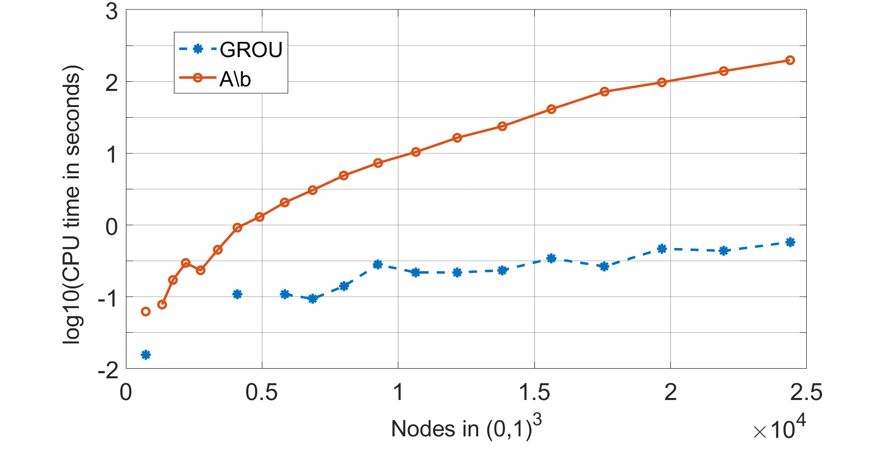
Figure 1: CPU time comparative to solve the discrete Poisson equation. For this numerical test, we have used a computer with the following characteristics: 11th Gen Intel(R) Core(TM) i7-11370H @ 3.30GHz, RAM 16,0 GB, 64 bit operating system; and a Matlab version R2021b ^matlab.

So, we will use this fact to study if, for a given generic square matrix, a characterization can be stated such that we can decide whether is either Laplacian-like or not. Clearly, under a positive answer, we expect that the analysis of the associated linear system $A\mathbf{x}=\mathbf{b}$ would be simpler. This kind of linear operator also exists in infinite dimensional vector spaces to describe evolution equations in tensor Banach spaces ¹⁴. Its main property is that the associated dynamical system has an invariant manifold, the manifold of elementary tensors (see ¹⁵ for the details about its manifold structure).

Thus, the goal of this paper is to obtain a complete description of this linear space of matrices, showing that is, in fact, a Lie subalgebra of $\mathbb{R}^{N\times N}$, and provide an algorithm in order to obtain the best approximation to this linear space, that is, to compute explicitly is the orthogonal projection on that space.

The paper is organized as follows: in Section 2, we introduce the linear subspace of Laplacian-like matrices and prove that it is also a matrix Lie sub-algebra associated to a particular Lie group. Then, in Section 3, we prove that any matrix is uniquely decomposed as the sum of a Laplacian matrix and a matrix which is the subspace generated by the identity matrix, and we show that any Laplacian matrix is a direct sum of some particular orthogonal subspaces. Section 4 is devoted, with the help of the results of the previous section, to propose an algorithm to explicitly compute the orthogonal projection onto the subspace of Laplacian-like matrices. To illustrate this result, we also give some numerical examples. Finally, in Section 5 some conclusions and final remarks are given.

2 The algebraic structure of Laplacian-Like matrices

First of all, we introduce some definitions, that will be used along this work.

Definition 2.1.

Let $A\in{\mathbb{R}}^{M\times N}.$ Then, the Fröbenius norm (or the Hilbert–Schmidt norm) is defined as

$$||A||_{F}=\sqrt{\sum_{i=1}^{M}\sum_{j=1}^{N}|a_{ij}|^{2}}=\sqrt{\mathrm{tr}\left(A^{\top}A\right)}.$$

The Fröbenius norm is the norm induced by the trace therefore, when $N=M$, we can work with the scalar product given by $\langle A,B\rangle=\mathrm{tr}\left(A^{\top}B\right)$. Let us observe that, in ${\mathbb{R}}^{N\times N}$,

1. $\langle A,B\rangle_{{\mathbb{R}}^{N\times N}}=\mathrm{tr}\left(A^{\top}B\right)$

2. $\langle A,\mathrm{id}_{N}\rangle_{{\mathbb{R}}^{N\times N}}=\mathrm{tr}(A)=\mathrm{tr}\left(A^{\top}\right)$

3. $\langle\mathrm{id}_{N},\mathrm{id}_{N}\rangle_{{\mathbb{R}}^{N\times N}}=||\mathrm{id}_{N}||_{F}^{2}=N.$

Given a linear subspace $\mathcal{U}\subset\mathbb{R}^{N\times N}$ we will denote:

1. the orthogonal complement of $\mathcal{U}$ in $\mathbb{R}^{N\times N}$ by

   $$\mathcal{U}^{\bot}=\left\{V\in\mathbb{R}^{N\times N}:\langle U,V\rangle_{\mathbb{R}^{N\times N}}=0\text{ for all }U\in\mathcal{U}\right\},$$

   and,

2. the orthogonal projection of ${\mathbb{R}}^{N\times N}$ on $\mathcal{U}$ as

   $$P_{\mathcal{U}}(V):=\arg\min_{U\in\mathcal{U}}\|U-V\|_{F},$$

   and hence

   $$P_{\mathcal{U}^{\bot}}=\mathrm{id}_{N}-P_{\mathcal{U}}.$$

Before defining a Laplacian-like matrix, we recall that the Kronecker product of two matrices $A\in{\mathbb{R}}^{N_{1}\times M_{1}}$, $B\in{\mathbb{R}}^{N_{2}\times M_{2}}$ is defined by

$$A\otimes B=\begin{pmatrix}A_{1,1}B&A_{1,2}B&\dots&A_{1,M_{1}}B\\ A_{2,1}B&A_{2,2}B&\dots&A_{2,M_{1}}B\\ \vdots&\vdots&\ddots&\vdots\\ A_{N_{1},1}B&A_{N_{1},2}B&\dots&A_{N_{1},M_{1}}B\\ \end{pmatrix}\in{\mathbb{R}}^{N_{1}N_{2}\times M_{1}M_{2}}.$$

Some of the well-known properties of the Kronecker product are:

1. $A\otimes(B\otimes C)=(A\otimes B)\otimes C$.

2. $(A+B)\otimes C=(A\otimes C)+(B\otimes C)$.

3. $AB\otimes CD=(A\otimes C)(B\otimes D)$.

4. $(A\otimes B)^{-1}=A^{-1}\otimes B^{-1}$.

5. $(A\otimes B)^{\top}=A^{\top}\otimes B^{\top}$.

6. $\mathrm{tr}(A\otimes B)=\mathrm{tr}(A)\mathrm{tr}(B).$

From the example given in the introduction, we observe that there is a particular type of matrices to solve high-dimensional linear systems for which the GROU algorithm works particularly well: very fast convergence and also a very good approximation of the solution. These are the so-called Laplacian-Like matrices that we define below.

Definition 2.2.

Given a matrix $A\in\mathbb{R}^{N\times N},$ where $N=n_{1}\cdots n_{d},$ we say that $A$ is a Laplacian-like matrix if there exist matrices $A_{i}\in{\mathbb{R}}^{n_{i}\times n_{i}}$ for $1\leq i\leq d$ be such that

$$A=\sum_{i=1}^{d}\mathrm{id}_{[n_{i}]}\otimes A_{i}\doteq\sum_{i=1}^{d}\mathrm{id}_{n_{1}}\otimes\dots\otimes\mathrm{id}_{n_{i-1}}\otimes A_{i}\otimes\mathrm{id}_{n_{i+1}}\otimes\dots\otimes\mathrm{id}_{n_{d}},$$ (2)

where $\mathrm{id}_{n_{j}}$ is the identity matrix of size $n_{j}\times n_{j}.$

It is not difficult to see that the set of Laplacian-like matrices is a linear subspace of $\mathbb{R}^{N\times N}$. From now on, we will denote by $\mathcal{L}\left({\mathbb{R}}^{N\times N}\right)$ the subspace of Laplacian-like matrices in ${\mathbb{R}}^{N\times N}$ for a fixed decomposition of $N=n_{1}\cdots n_{d}$.

These matrices can be easily related to the classical Laplacian operator ^{16, 17} by writing:

$$\frac{\partial^{2}}{\partial x_{i}^{2}}=\frac{\partial^{0}}{\partial x_{1}^{0}}\otimes\dots\otimes\frac{\partial^{0}}{\partial x_{i-1}^{0}}\otimes\frac{\partial^{2}}{\partial x_{i}^{2}}\otimes\frac{\partial^{0}}{\partial x_{i+1}^{0}}\otimes\dots\otimes\frac{\partial^{0}}{\partial x_{d}^{0}}$$

and where $\frac{\partial^{0}}{\partial x_{j}^{0}}$ is the identity operator for functions in the variable $x_{j}$ for $j\neq i$.

As the next numerical example shows, matrices written as in (2) provides very good performance of the GROU algorithm. In Figure 2 we give a comparison of the speed of convergence to solve a linear system $A\mathbf{x}=\mathbf{b}$, where for each fixed size, we randomly generated two full-rank matrices: one given in the classical form and a Laplacian-like matrix. Both systems were solved following Algorithm 1.

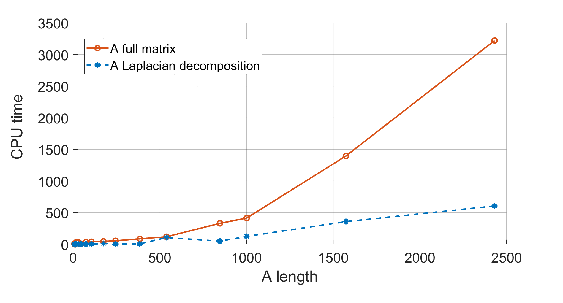
Figure 2: CPU time comparative to solve an $A\mathbf{x}=\mathbf{b}$ problem. This graph has been generated by using the following data in Algorithm 1: $\texttt{tol}=2.22e-6$; $\varepsilon=1.0e-06$; $\texttt{rank\_max}=3000$; (an $\texttt{iter-max}=15$ was used to perform an ALS strategy); and the matrices have been randomly generated for each different size, in Laplacian and classical form. The characteristics of the computer used here are the same as in the case of Figure 1.

The above results, together with the previous Poisson example given in the introduction, motivate the interest to know for a given matrix $A\in\mathbb{R}^{N\times N}$ how far it is from the linear subspace of Laplacian-like matrices. More precisely, we are interested in decomposing any matrix $A$ as a sum of two orthogonal matrices $L$ and $L^{\bot},$ where $L$ is in $\mathcal{L}(\mathbb{R})$ and $L^{\bot}$ in $\mathcal{L}(\mathbb{R})^{\bot}.$ Clearly, if we obtain that $L^{\bot}=0,$ that is, $A\in\mathcal{L}(\mathbb{R}),$ then we can solve any associated linear system by means of the GROU algorithm.

Recall that the set of matrices $\mathbb{R}^{N\times N}$ is a Lie Algebra that appears as the tangent space at the identity matrix of the linear general group $GL(\mathbb{R}^{N}),$ a Lie group composed by the non-singular matrices of $\mathbb{R}^{N\times N}$ (see ¹⁸). Furthermore, the exponential map

$$\exp:\mathbb{R}^{N\times N}\longrightarrow GL(\mathbb{R}^{N}),\quad A\mapsto\exp(A)=\sum_{n=0}^{\infty}\frac{A^{n}}{n!}$$

is well-defined, however it is not surjective because $\det(\exp(A))=e^{\mathrm{tr}(A)}>0.$ Any linear subspace $\mathfrak{h}\subset\mathbb{R}^{N\times N}$ is a Lie-subalgebra if for all $A,B\in\mathfrak{h}$ its Lie crochet is also in $\mathfrak{h},$ that is, $[A,B]=AB-BA\in\mathfrak{h}$.

The linear space $\mathcal{L}(\mathbb{R}^{N\times N})$ is more than a linear subspace of $\mathbb{R}^{N\times N},$ it is also a Lie sub-algebra of $\mathbb{R}^{N\times N}$ as the next result shows.

Proposition 2.3.

Assume $\mathbb{R}^{N\times N},$ where where $N=n_{1}\cdots n_{d}.$ Then the following statements hold.

1. The linear subspace $\mathcal{L}(\mathbb{R}^{N\times N})$ is a Lie subalgebra of the matrix Lie algebra $R^{N\times N}.$

2. The matrix group

   $$\mathfrak{L}(\mathbb{R}^{N\times N})=\left\{\bigotimes_{i=1}^{d}A_{i}:A_{i}\in GL(\mathbb{R}^{n_{i}})\text{ for }1\leq i\leq d\right\}$$

   is a Lie subgroup of $GL\left(\mathbb{R}^{N}\right).$

3. The exponential map

   $$\exp:\mathcal{L}(\mathbb{R}^{N\times N})\longrightarrow\mathfrak{L}(\mathbb{R}^{N\times N}),\quad\sum_{i=1}^{d}\mathrm{id}_{n_{1}}\otimes\dots\otimes\mathrm{id}_{n_{i-1}}\otimes A_{i}\otimes\mathrm{id}_{n_{i+1}}\otimes\dots\otimes\mathrm{id}_{n_{d}}\mapsto\bigotimes_{i=1}^{d}\exp(A_{i}),$$

   is well defined.

Proof 2.4.

(a) To prove the first statement, take $A,B\in\mathcal{L}(\mathbb{R}^{N\times N}).$ Then there exist matrices $A_{i},B_{i}\in{\mathbb{R}}^{n_{i}\times n_{i}}$ for $1\leq i\leq d$ be such that

$$A=\sum_{i=1}^{d}\mathrm{id}_{n_{1}}\otimes\dots\otimes\mathrm{id}_{n_{i-1}}\otimes A_{i}\otimes\mathrm{id}_{n_{i+1}}\otimes\dots\otimes\mathrm{id}_{n_{d}},$$

and

$$B=\sum_{i=1}^{d}\mathrm{id}_{n_{1}}\otimes\dots\otimes\mathrm{id}_{n_{i-1}}\otimes B_{i}\otimes\mathrm{id}_{n_{i+1}}\otimes\dots\otimes\mathrm{id}_{n_{d}}.$$

Observe, that for $i<j$

$$\left(\mathrm{id}_{n_{1}}\otimes\dots\otimes\mathrm{id}_{n_{i-1}}\otimes A_{i}\otimes\mathrm{id}_{n_{i+1}}\otimes\dots\otimes\mathrm{id}_{n_{d}}\right)\left(\mathrm{id}_{n_{1}}\otimes\dots\otimes\mathrm{id}_{n_{j-1}}\otimes B_{j}\otimes\mathrm{id}_{n_{j+1}}\otimes\dots\otimes\mathrm{id}_{n_{d}}\right)$$

and

$$\left(\mathrm{id}_{n_{1}}\otimes\dots\otimes\mathrm{id}_{n_{j-1}}\otimes B_{j}\otimes\mathrm{id}_{n_{j+1}}\otimes\dots\otimes\mathrm{id}_{n_{d}}\right)\left(\mathrm{id}_{n_{1}}\otimes\dots\otimes\mathrm{id}_{n_{i-1}}\otimes A_{i}\otimes\mathrm{id}_{n_{i+1}}\otimes\dots\otimes\mathrm{id}_{n_{d}}\right)$$

both products are equal to

$$\mathrm{id}_{n_{1}}\otimes\dots\otimes\mathrm{id}_{n_{i-1}}\otimes A_{i}\otimes\mathrm{id}_{n_{i+1}}\otimes\cdots\otimes\mathrm{id}_{n_{j-1}}\otimes B_{j}\otimes\mathrm{id}_{n_{j+1}}\otimes\dots\mathrm{id}_{n_{d}}.$$

A similar expression is obtained for $i>j.$ Thus,

$$\left[\mathrm{id}_{n_{1}}\otimes\dots\otimes\mathrm{id}_{n_{i-1}}\otimes A_{i}\otimes\mathrm{id}_{n_{i+1}}\otimes\dots\otimes\mathrm{id}_{n_{d}},\mathrm{id}_{n_{1}}\otimes\dots\otimes\mathrm{id}_{n_{j-1}}\otimes B_{j}\otimes\mathrm{id}_{n_{j+1}}\otimes\dots\otimes\mathrm{id}_{n_{d}}\right]=0$$

for all $i\neq j.$

On the other hand, for $i=j$ we have

$$\left(\mathrm{id}_{n_{1}}\otimes\dots\otimes\mathrm{id}_{n_{i-1}}\otimes A_{i}\otimes\mathrm{id}_{n_{i+1}}\otimes\dots\otimes\mathrm{id}_{n_{d}}\right)\left(\mathrm{id}_{n_{1}}\otimes\dots\otimes\mathrm{id}_{n_{i-1}}\otimes B_{i}\otimes\mathrm{id}_{n_{i+1}}\otimes\dots\otimes\mathrm{id}_{n_{d}}\right)$$

is equal to

$$\mathrm{id}_{n_{1}}\otimes\dots\otimes\mathrm{id}_{n_{i-1}}\otimes A_{i}B_{i}\otimes\mathrm{id}_{n_{i+1}}\otimes\dots\otimes\mathrm{id}_{n_{d}}$$

and

$$\left(\mathrm{id}_{n_{1}}\otimes\dots\otimes\mathrm{id}_{n_{i-1}}\otimes B_{i}\otimes\mathrm{id}_{n_{i+1}}\otimes\dots\otimes\mathrm{id}_{n_{d}}\right)\left(\mathrm{id}_{n_{1}}\otimes\dots\otimes\mathrm{id}_{n_{i-1}}\otimes A_{i}\otimes\mathrm{id}_{n_{i+1}}\otimes\dots\otimes\mathrm{id}_{n_{d}}\right)$$

is equal to

$$\mathrm{id}_{n_{1}}\otimes\dots\otimes\mathrm{id}_{n_{i-1}}\otimes B_{i}A_{i}\otimes\mathrm{id}_{n_{i+1}}\otimes\dots\otimes\mathrm{id}_{n_{d}}.$$

Thus,

$$\left[\mathrm{id}_{n_{1}}\otimes\dots\otimes\mathrm{id}_{n_{i-1}}\otimes A_{i}\otimes\mathrm{id}_{n_{i+1}}\otimes\dots\otimes\mathrm{id}_{n_{d}},\mathrm{id}_{n_{1}}\otimes\dots\otimes\mathrm{id}_{n_{i-1}}\otimes B_{i}\otimes\mathrm{id}_{n_{i+1}}\otimes\dots\otimes\mathrm{id}_{n_{d}}\right]$$

is equal to

$$\mathrm{id}_{n_{1}}\otimes\dots\otimes\mathrm{id}_{n_{i-1}}\otimes(A_{i}B_{i}-B_{i}A_{i})\otimes\mathrm{id}_{n_{i+1}}\otimes\dots\otimes\mathrm{id}_{n_{d}},$$

that is,

$$\mathrm{id}_{n_{1}}\otimes\dots\otimes\mathrm{id}_{n_{i-1}}\otimes[A_{i},B_{i}]\otimes\mathrm{id}_{n_{i+1}}\otimes\dots\otimes\mathrm{id}_{n_{d}}.$$

Here $[A_{i},B_{i}]$ is the Lie crochet in $\mathbb{R}^{n_{i}\times n_{i}}.$

In consequence, from all said above, we conclude

$$[A,B] =\sum_{i=1}^{d}\sum_{j=1}^{d}\left[\mathrm{id}_{n_{1}}\otimes\dots\otimes\mathrm{id}_{n_{i-1}}\otimes A_{i}\otimes\mathrm{id}_{n_{i+1}}\otimes\dots\otimes\mathrm{id}_{n_{d}},\mathrm{id}_{n_{1}}\otimes\dots\otimes\mathrm{id}_{n_{i-1}}\otimes B_{j}\otimes\mathrm{id}_{n_{i+1}}\otimes\dots\otimes\mathrm{id}_{n_{d}}\right]$$

$$=\sum_{i=1}^{d}\mathrm{id}_{n_{1}}\otimes\dots\otimes\mathrm{id}_{n_{i-1}}\otimes[A_{i},B_{i}]\otimes\mathrm{id}_{n_{i+1}}\otimes\dots\otimes\mathrm{id}_{n_{d}}\in\mathcal{L}\left(\mathbb{R}^{N\times N}\right).$$

This proves that $\mathcal{L}(\mathbb{R}^{N\times N})$ is a Lie sub-algebra of $\mathbb{R}^{N\times N}.$

(b) It is not difficult to see that $\mathfrak{L}(\mathbb{R}^{N\times N})$ is a subgroup of $GL(\mathbb{R}^{N}).$ From Theorem 19.18 in ¹⁸, to prove that $\mathfrak{L}(\mathbb{R}^{N\times N})$ is a Lie subgroup of $GL(\mathbb{R}^{N})$ we only need to show that $\mathfrak{L}(\mathbb{R}^{N\times N})$ is a closed set in $GL(\mathbb{R}^{N}).$ This follows from the fact that the map

$$\Phi:GL(\mathbb{R}^{n_{1}})\times\cdots\times GL(\mathbb{R}^{n_{d}})\longrightarrow GL(\mathbb{R}^{N})\quad(A_{1},\cdots,A_{d})\mapsto\bigotimes_{i=1}^{d}A_{i}$$

is continuous. Assume that there exists a sequence, $\{A_{n}\}_{n\in\mathbb{N}}\subset\mathfrak{L}(\mathbb{R}^{N\times N})$ convergent to $A\in GL(\mathbb{R}^{n}).$ Then the sequence $\{A_{n}\}_{n\in\mathbb{N}}$ is bounded. Since there exists a sequence $\{(A_{1}^{(n)},\ldots,A_{d}^{(n)})\}_{n\in\mathbb{N}}\subset GL(\mathbb{R}^{n_{1}})\times\cdots\times GL(\mathbb{R}^{n_{d}})$ such that $A_{n}=\bigotimes_{j=1}^{d}A_{j}^{(n)},$ the sequence $\{(A_{1}^{(n)},\ldots,A_{d}^{(n)})\}_{n\in\mathbb{N}}$ is also bounded. Thus, there exists a convergent sub-sequence, also denoted by $\{(A_{1}^{(n)},\ldots,A_{d}^{(n)})\}_{n\in\mathbb{N}},$ to $(A_{1},\ldots,A_{d})\in GL(\mathbb{R}^{n_{1}})\times\cdots\times GL(\mathbb{R}^{n_{d}}).$ The continuity of $\Phi,$ implies that $A=\bigotimes_{i=1}^{d}A_{i}.$ Thus $\mathfrak{L}(\mathbb{R}^{N\times N})$ is closed in $GL(\mathbb{R}^{N}),$ and hence a Lie subgroup.

(c) From Lemma 4.169(b)⁸, the following equality

$$\exp\left(\sum_{i=1}^{d}\mathrm{id}_{n_{1}}\otimes\dots\otimes\mathrm{id}_{n_{i-1}}\otimes A_{i}\otimes\mathrm{id}_{n_{i+1}}\otimes\dots\otimes\mathrm{id}_{n_{d}}\right)=\bigotimes_{i=1}^{d}\exp(A_{i})$$

holds. Thus, the exponential map is well defined. This ends the proof of the proposition.

We conclude this section describing in a more detail the structure of matrices $A\in{\mathbb{R}}^{N\times N}$ for which there exists $A_{i}\in{\mathbb{R}}^{n_{i}\times n_{i}}$ for $1\leq i\leq d$ such that

$$A=\sum_{i=1}^{d}\mathrm{id}_{n_{1}}\otimes\dots\mathrm{id}_{n_{i-1}}\otimes A_{i}\otimes\mathrm{id}_{n_{i+1}}\otimes\dots\otimes\mathrm{id}_{n_{d}}.$$

For dealing easily with Laplacian-like matrices, we introduce the following notation. For each $1<i\leq d$ consider the integer number $n_{1}n_{2}\cdots n_{i-1}.$ Then, we will denote by

$$\left(\begin{array}[]{cccc}\star&\star&\cdots&\star\\ \star&\star&\cdots&\star\\ \vdots&\vdots&\ddots&\vdots\\ \star&\star&\cdots&\star\end{array}\right)_{n_{1}n_{2}\cdots n_{i-1}\times n_{1}n_{2}\cdots n_{i-1}}$$

a block square matrix composed by $n_{1}n_{2}\cdots n_{i-1}\times n_{1}n_{2}\cdots n_{i-1}$-blocks. Then, we observe, that for $1<i<d,$ we can write

$$\mathrm{id}_{n_{1}}\otimes\dots\mathrm{id}_{n_{i-1}}\otimes A_{i}\otimes\mathrm{id}_{n_{i+1}}\otimes\dots\otimes\mathrm{id}_{n_{d}}=\mathrm{id}_{n_{1}\cdots n_{i-1}}\otimes A_{i}\otimes\mathrm{id}_{n_{i+1}\cdots n_{d}}.$$

Since

$$A_{i}\otimes\mathrm{id}_{n_{i+1}\cdots n_{d}}=\begin{pmatrix}(A_{i})_{1,1}\mathrm{id}_{n_{i+1}\cdots n_{d}}\phantom{a}&(A_{i})_{1,2}\mathrm{id}_{n_{i+1}\cdots n_{d}}\phantom{a}&\dots\phantom{a}&(A_{i})_{1,n_{i}}\mathrm{id}_{n_{i+1}\cdots n_{d}}\\ (A_{i})_{2,1}\mathrm{id}_{n_{i+1}\cdots n_{d}}\phantom{a}&(A_{i})_{2,2}\mathrm{id}_{n_{i+1}\cdots n_{d}}\phantom{a}&\dots\phantom{a}&(A_{i})_{2,n_{i}}\mathrm{id}_{n_{i+1}\cdots n_{d}}\\ \vdots\phantom{a}&\vdots\phantom{a}&\ddots\phantom{a}&\vdots\\ (A_{i})_{n_{i},1}\mathrm{id}_{n_{i+1}\cdots n_{d}}\phantom{a}&(A_{i})_{n_{i},2}\mathrm{id}_{n_{i+1}\cdots n_{d}}\phantom{a}&\dots\phantom{a}&(A_{i})_{n_{i},n_{i}}\mathrm{id}_{n_{i+1}\cdots n_{d}}\\ \end{pmatrix},$$

then

$$\phantom{a}\mathrm{id}_{n_{1}\cdots n_{i-1}}\otimes A_{i}\otimes\mathrm{id}_{n_{i+1}\cdots n_{d}}=\begin{pmatrix}A_{i}\otimes\mathrm{id}_{n_{i+1}\cdots n_{d}}\phantom{a}&O_{i}\otimes\mathrm{id}_{n_{i+1}\cdots n_{d}}\phantom{a}&\cdots\phantom{a}&O_{i}\otimes\mathrm{id}_{n_{i+1}\cdots n_{d}}\\ O_{i}\otimes\mathrm{id}_{n_{i+1}\cdots n_{d}}\phantom{a}&A_{i}\otimes\mathrm{id}_{n_{i+1}\cdots n_{d}}\phantom{a}&\cdots\phantom{a}&O_{i}\otimes\mathrm{id}_{n_{i+1}\cdots n_{d}}\\ \vdots\phantom{a}&\vdots\phantom{a}&\ddots\phantom{a}&\vdots\\ O_{i}\otimes\mathrm{id}_{n_{i+1}\cdots n_{d}}\phantom{a}&O_{i}\otimes\mathrm{id}_{n_{i+1}\cdots n_{d}}\phantom{a}&\cdots\phantom{a}&A_{i}\otimes\mathrm{id}_{n_{i+1}\cdots n_{d}}\end{pmatrix}_{n_{1}n_{2}\cdots n_{i-1}\times n_{1}n_{2}\cdots n_{i-1}},$$

where $O_{i}$ denotes the zero matrix in ${\mathbb{R}}^{n_{i}\times n_{i}}$ for $1\leq i\leq d.$ To conclude, we have the following cases

$$A_{1}\otimes\mathrm{id}_{n_{2}\cdots n_{d}}=\begin{pmatrix}(A_{1})_{1,1}\mathrm{id}_{n_{2}\cdots n_{d}}\phantom{a}&(A_{1})_{1,2}\mathrm{id}_{n_{2}\cdots n_{d}}\phantom{a}&\dots&(A_{1})_{1,n_{1}}\mathrm{id}_{n_{2}\cdots n_{d}}\\ (A_{1})_{2,1}\mathrm{id}_{n_{2}\cdots n_{d}}\phantom{a}&(A_{1})_{2,2}\mathrm{id}_{n_{2}\cdots n_{d}}\phantom{a}&\dots\phantom{a}&(A_{1})_{2,n_{1}}\mathrm{id}_{n_{2}\cdots n_{d}}\\ \vdots\phantom{a}&\vdots\phantom{a}&\ddots\phantom{a}&\vdots\\ (A_{1})_{n_{1},1}\mathrm{id}_{n_{2}\cdots n_{d}}\phantom{a}&(A_{1})_{n_{1},2}\mathrm{id}_{n_{2}\cdots n_{d}}\phantom{a}&\dots\phantom{a}&(A_{1})_{n_{1},n_{1}}\mathrm{id}_{n_{2}\cdots n_{d}}\\ \end{pmatrix}$$

and

$$\mathrm{id}_{n_{1}\cdots n_{d-1}}\otimes A_{d}=\begin{pmatrix}A_{d}&O_{d}&\cdots&O_{d}\\ O_{d}&A_{d}&\cdots&O_{d}\\ \vdots&\vdots&\ddots&\vdots\\ O_{d}&O_{d}&\cdots&A_{d}\end{pmatrix}_{n_{1}n_{2}\cdots n_{d-1}\times n_{1}n_{2}\cdots n_{d-1}}.$$

We wish to point out that the above operations are widely used in quantum computing.

3 A decomposition of the linear space of Laplacian-like matrices

We start by introducing some definitions and preliminary results needed to give an interesting decomposition of the linear space of Laplacian-like matrices. The next lemma lets us show how is the decomposition of ${\mathbb{R}}^{N\times N}$ as a direct sum of $\mathrm{span}\{\mathrm{id}_{N}\}$ and its orthogonal space.

Lemma 3.1.

Consider $\left({\mathbb{R}}^{N\times N},\|\cdot\|_{F}\right)$ as a Hilbert space. Then there exists a decomposition

$${\mathbb{R}}^{N\times N}=\mathrm{span}\{\mathrm{id}_{N}\}\oplus\mathrm{span}\{\mathrm{id}_{N}\}^{\bot},$$

where $\mathrm{span}\{\mathrm{id}_{N}\}^{\bot}=\{A\in{\mathbb{R}}^{N\times N}:\mathrm{tr}(A)=0\}.$ Moreover, the orthogonal projection from ${\mathbb{R}}^{N\times N}$ on $\mathrm{span}\{\mathrm{id}_{N}\}$ is given by

$$P_{\mathrm{span}\{\mathrm{id}_{N}\}}(A)=\frac{\mathrm{tr}(A)}{N}\,\mathrm{id}_{N},$$

and hence for each $A\in{\mathbb{R}}^{N\times N}$ we have the following decomposition,

$$A=\frac{\mathrm{tr}(A)}{N}\,\mathrm{id}_{N}+\left(A-\frac{\mathrm{tr}(A)}{N}\mathrm{id}_{N}\right),$$

where $\left(A-\frac{\mathrm{tr}(A)}{N}\mathrm{id}_{N}\right)\in\mathrm{span}\{\mathrm{id}_{N}\}^{\bot}.$

Proof 3.2.

The lemma follows from the fact that

$$P_{\mathrm{id}_{N}}(A)=\frac{\langle\mathrm{id}_{N},A\rangle_{{\mathbb{R}}^{N\times N}}}{\|\mathrm{id}_{N}\|_{F}^{2}}\,\mathrm{id}_{n}=\frac{\mathrm{tr}(A)}{N}\,\mathrm{id}_{N},$$

is the orthogonal projection onto $\mathrm{span}\{\mathrm{id}_{N}\}.$

Now, we consider the matrix space $\mathbb{R}^{N\times N}$ where $N=n_{1}\cdots n_{d},$ and hence $\mathbb{R}^{N\times N}=\bigotimes_{i=1}^{d}{\mathbb{R}}^{n_{i}\times n_{i}}$ can be considered as a tensor space. Then, for rank-one tensors $A=A_{1}\otimes\dots\otimes A_{d}$ and $B=B_{1}\otimes\dots\otimes B_{d}$ where $A_{i},B_{i}\in{\mathbb{R}}^{n_{i}\times n_{i}},$ we have

$$\langle A,B\rangle_{{\mathbb{R}}^{N\times N}} =\langle A_{1}\otimes\dots\otimes A_{d},B_{1}\otimes\dots\otimes B_{d}\rangle_{{\mathbb{R}}^{N\times N}}=\mathrm{tr}((A_{1}\otimes\dots\otimes A_{d})^{T}(B_{1}\otimes\dots\otimes B_{d}))$$

$$=\mathrm{tr}((A_{1}^{T}\otimes\dots\otimes A_{d}^{T})(B_{1}\otimes\dots\otimes B_{d}))=\mathrm{tr}(A_{1}^{T}B_{1}\otimes\dots\otimes A_{d}^{T}B_{d})$$

$$=\prod_{i=1}^{d}\mathrm{tr}(A_{i}^{\top}B_{i})=\prod_{i=1}^{d}\langle A_{i},B_{i}\rangle_{{\mathbb{R}}^{n_{i}\times n_{i}}}.$$

Thus, the inner product $\langle\cdot,\cdot\rangle_{\mathbb{R}^{N\times N}}$ satisfies

$$\langle\mathrm{id}_{[n_{i}]}\otimes A_{i},\mathrm{id}_{[n_{i}]}\otimes B_{i}\rangle_{{\mathbb{R}}^{N\times N}}=\mathrm{tr}(A_{i}^{\top}B_{i})\prod_{\begin{subarray}{c}j=1\\ j\neq i\end{subarray}}^{d}n_{j},$$ (3)

and $\|A\|_{F}=\sqrt{\langle A,A\rangle_{{\mathbb{R}}^{N\times N}}},$ is called a tensor-norm.

The next result gives a first characterization of the linear space $\mathcal{L}\left(\mathbb{R}^{N\times N}\right).$

Theorem 3.3.

Let ${\mathbb{R}}^{N\times N},$ where $N=n_{1}\cdots n_{d}.$ Then

$$\mathcal{L}\left(\mathbb{R}^{N\times N}\right)=\mathrm{span}\,\{\mathrm{id}_{N}\}\oplus\Delta,$$ (4)

where $\Delta=(\mathrm{span}\{\mathrm{id}_{N}\}^{\bot}\cap\mathcal{L}({\mathbb{R}}^{N\times N})).$ Furthermore, $\mathcal{L}({\mathbb{R}}^{N\times N})^{\bot}$ is a subspace of $\mathrm{span}\{\mathrm{id}_{N}\}^{\bot}.$

Proof 3.4.

Assume that a given matrix $A\in\mathbb{R}^{N\times N}$ can be written as in (2). and denote each component in the sum representation of $A,$ by $L_{i}=\mathrm{id}_{[n_{i}]}\otimes A_{i},$ where $A_{i}\in{\mathbb{R}}^{n_{i}\times n_{i}}$ for $1\leq i\leq d.$ Then $L_{i}\in\mathrm{span}\{\mathrm{id}_{[n_{i}]}\}\otimes{\mathbb{R}}^{n_{i}\times n_{i}}$ for $1\leq i\leq d,$ and in consequence,

$$\sum_{i=1}^{d}\mathrm{span}\{\mathrm{id}_{[n_{i}]}\}\otimes{\mathbb{R}}^{n_{i}\times n_{i}}=\mathcal{L}\left(\mathbb{R}^{N\times N}\right).$$

Thus, $\mathrm{span}\{\mathrm{id}_{N}\}\subset\mathcal{L}\left(\mathbb{R}^{N\times N}\right),$ and, by Lemma 3.1, we have the following decomposition

$$\mathcal{L}\left(\mathbb{R}^{N\times N}\right)=\Delta\oplus\mathrm{span}\{\mathrm{id}_{N}\}.$$ (5)

where $\Delta=\left(\mathrm{span}\{\mathrm{id}_{N}\}^{\bot}\cap\mathcal{L}({\mathbb{R}}^{N\times N})\right).$ The last statement is consequence of Lemma 3.1. This ends the theorem.

Now, given any square matrix in ${\mathbb{R}}^{N\times N},$ we would like to project it onto $\mathcal{L}(\mathbb{R}^{N\times N})$ to obtain its Laplacian approximation. To compute this approximation explicitly, the following result, which is a consequence of the above theorem, will be useful.

Corollary 3.5.

Assume $\mathbb{R}^{N\times N},$ with $N=n_{1}\cdots n_{d}\in{\mathbb{N}}.$ Then

$$P_{\mathcal{L}({\mathbb{R}}^{N\times N})}=P_{\mathrm{span}\{\mathrm{id}_{N}\}}+P_{\Delta},$$

that is, for all $A\in{\mathbb{R}}^{N\times N}$ it holds

$$P_{\mathcal{L}({\mathbb{R}}^{N\times N})}(A)=\frac{\mathrm{tr}(A)}{N}\,\mathrm{id}_{N}+P_{\Delta}(A).$$

Next, we need to characterize $\Delta$ in order to explicitly construct the orthogonal projection onto $\mathcal{L}(\mathbb{R}^{N\times N})$. From the proof of the Theorem 3.3 we see that the linear subspaces given by

$$\mathrm{span}\{\mathrm{id}_{N}\}^{\bot}\cap\mathrm{span}\{\mathrm{id}_{[n_{i}]}\}\otimes{\mathbb{R}}^{n_{i}\times n_{i}},$$

for $1\leq i\leq d,$ are of interest to characterize $\Delta$ as the next result shows.

Theorem 3.6.

Let $\mathbb{R}^{N\times N}$ with $N=n_{1}\cdots n_{d}\in{\mathbb{N}},$ and let $\mathrm{span}\{\mathrm{id}_{N}\}^{\perp_{i}}$ be the orthogonal complement of $\mathrm{span}\{\mathrm{id}_{N}\}$ in the linear subspace $\mathrm{span}\{\mathrm{id}_{[n_{i}]}\}\otimes{\mathbb{R}}^{n_{i}\times n_{i}}$ for $1\leq i\leq d$. Then,

$$\Delta=\bigoplus_{i=1}^{d}\mathrm{span}\{\mathrm{id}_{N}\}^{\perp_{i}}.$$ (6)

Furthermore, a matrix $A$ belongs to $\Delta$ if and only if it has the form

$$A=\sum_{i=1}^{d}\mathrm{id}_{n_{1}}\otimes\dots\mathrm{id}_{n_{i-1}}\otimes A_{i}\otimes\mathrm{id}_{n_{i+1}}\otimes\dots\otimes\mathrm{id}_{n_{d}},\quad\text{with}\quad\mathrm{tr}(A_{i})=0,\;i=1,\dots,d.$$

Proof 3.7.

First, we take into account that $\mathrm{span}\{\mathrm{id}_{[n_{i}]}\}\otimes{\mathbb{R}}^{n_{i}\times n_{i}}$ a linear subspace of $\mathcal{L}(\mathbb{R}^{N\times N})$ linearly isomorphic to the matrix space ${\mathbb{R}}^{n_{i}\times n_{i}}.$ Thus, motivated by Lemma 3.1 applied on $\mathbb{R}^{n_{i}\times n_{i}}$, we write

$$\mathrm{span}\{\mathrm{id}_{[n_{i}]}\}\otimes{\mathbb{R}}^{n_{i}\times n_{i}} =\mathrm{span}\{\mathrm{id}_{[n_{i}]}\}\oplus(\mathrm{span}\{\mathrm{id}_{n_{i}}\}\otimes\mathrm{span}\{\mathrm{id}_{n_{i}}\}^{\bot})$$

$$=(\mathrm{span}\{\mathrm{id}_{[n_{i}]}\}\otimes\mathrm{span}\{\mathrm{id}_{n_{i}}\})\oplus(\mathrm{span}\{\mathrm{id}_{[n_{i}]}\}\otimes\mathrm{span}\{\mathrm{id}_{n_{i}}\}^{\bot})$$

$$=\mathrm{span}\{\mathrm{id}_{N}\}\oplus\mathrm{span}\{\mathrm{id}_{N}\}^{\perp_{i}},$$

Since $\mathrm{span}\{\mathrm{id}_{N}\}^{\perp_{i}}=\mathrm{span}\{\mathrm{id}_{[n_{i}]}\}\otimes\mathrm{span}\{\mathrm{id}_{n_{i}}\}^{\bot},$ we claim that it is the orthogonal complement of the linear subspace generated by the identity matrix $\mathrm{id}_{N}=\mathrm{id}_{[n_{i}]}\otimes\mathrm{id}_{n_{i}}$ in the linear subspace $\mathrm{id}_{[n_{i}]}\otimes{\mathbb{R}}^{n_{i}\times n_{i}}.$ To prove the claim, observe that for $\mathrm{id}_{[n_{i}]}\otimes A_{i}\in\mathrm{span}\{\mathrm{id}_{N}\}^{\perp_{i}}$ $(1\leq i\leq d),$ by using (3), it holds

$$\langle\mathrm{id}_{[n_{i}]}\otimes A_{i},\mathrm{id}_{N}\rangle_{{\mathbb{R}}^{N\times N}}=\langle\mathrm{id}_{[n_{i}]}\otimes A_{i},\mathrm{id}_{[n_{i}]}\otimes\mathrm{id}_{n_{i}}\rangle_{{\mathbb{R}}^{N\times N}}=\mathrm{tr}(A_{i})\prod_{\begin{subarray}{c}j=1\\ j\neq i\end{subarray}}^{d}n_{j}=0,$$

because $A_{i}\in\mathrm{span}\{\mathrm{id}_{n_{i}}\}^{\bot}$ and hence $\mathrm{tr}(A_{i})=0,$ for $1\leq i\leq d.$ Thus, the claim follows and

$$\begin{matrix}\begin{aligned} \mathrm{span}\{\mathrm{id}_{N}\}^{\perp_{i}}&=\{\mathrm{id}_{[n_{i}]}\otimes A_{i}\in\mathrm{span}\{\mathrm{id}_{[n_{i}]}\}\otimes{\mathbb{R}}^{n_{i}\times n_{i}}\,:\,\mathrm{tr}(A_{i})=0\}\\ &=\left\{\mathrm{id}_{[n_{i}]}\otimes A_{i}\in\mathrm{span}\{\mathrm{id}_{[n_{i}]}\}\otimes{\mathbb{R}}^{n_{i}\times n_{i}}:\langle\mathrm{id}_{[n_{i}]}\otimes A_{i},\mathrm{id}_{N}\rangle_{{\mathbb{R}}^{N\times N}}=0\right\}.\end{aligned}\end{matrix}$$

To prove (6), we first consider $1\leq i<j\leq d,$ and take $\mathrm{id}_{[n_{k}]}\otimes A_{k}\in\mathrm{span}\{\mathrm{id}_{N}\}^{\perp_{k}}$ for $k=i,j.$ Then the inner product satisfies

$$\langle\mathrm{id}_{[n_{i}]}\otimes A_{i},\mathrm{id}_{[n_{j}]}\otimes A_{j}\rangle_{{\mathbb{R}}^{N\times N}} =\mathrm{tr}\left((\mathrm{id}_{[n_{i}]}\otimes A_{i})^{T}(\mathrm{id}_{[n_{j}]}\otimes A_{j})\right)=\mathrm{tr}\left((\mathrm{id}_{[n_{i}]}\otimes A_{i}^{T})(\mathrm{id}_{[n_{j}]}\otimes A_{j})\right)$$

$$=\mathrm{tr}\left(\mathrm{id}_{n_{1}}\otimes\mathrm{id}_{n_{i-1}}\otimes A_{i}^{T}\otimes\mathrm{id}_{n_{i+1}}\otimes\cdots\otimes\mathrm{id}_{n_{j-1}}\otimes A_{j}\otimes\mathrm{id}_{n_{j+1}}\otimes\cdots\otimes\mathrm{id}_{n_{d}}\right)$$

$$=\prod_{\stackrel{{\scriptstyle\ell=1}}{{\ell\neq i,j}}}^{d}\langle\mathrm{id}_{\ell},\mathrm{id}_{\ell}\rangle_{{\mathbb{R}}^{n_{\ell}\times n_{\ell}}}\mathrm{tr}(A_{i})\mathrm{tr}(A_{j})=0,$$

because $\mathrm{tr}(A_{i})=\mathrm{tr}(A_{j})=0.$ The same equality holds for $j<i.$ Thus, we conclude that $\mathrm{span}\{\mathrm{id}_{N}\}^{\perp_{i}}$ is orthogonal to $\mathrm{span}\{\mathrm{id}_{N}\}^{\perp_{j}}$ for all $i\neq j.$ So, the subspace

$$\Delta^{\prime}=\bigoplus_{i=1}^{d}\mathrm{span}\{\mathrm{id}_{N}\}^{\perp_{i}},$$

is well defined and it is a subspace of $\mathcal{L}(\mathbb{R}^{N\times N}).$

To conclude the proof (6), we will show that $\Delta^{\prime}=\Delta.$ Since, for each $1\leq i\leq d,$ $\mathrm{span}\{\mathrm{id}_{N}\}^{\perp_{i}}$ is orthogonal to $\mathrm{span}\{\mathrm{id}_{N}\}$ we have

$$\mathrm{span}\{\mathrm{id}_{N}\}\oplus\Delta^{\prime}\subset\mathcal{L}(\mathbb{R}^{N\times N}).$$

To obtain the equality, take $A\in\mathcal{L}(\mathbb{R}^{N\times N}).$ Then there exists $A_{i}\in{\mathbb{R}}^{n_{i}\times n_{i}}$ for $1\leq i\leq d$ be such that

$$A=\sum_{i=1}^{d}\mathrm{id}_{[n_{i}]}\otimes A_{i}.$$

From Lemma 3.1 we can write

$$A_{i}=\frac{\mathrm{tr}(A_{i})}{n_{i}}\,\mathrm{id}_{n_{i}}+\left(A_{i}-\frac{\mathrm{tr}(A_{i})}{n_{i}}\,\mathrm{id}_{n_{i}}\right)$$

for each $1\leq i\leq d.$ Then,

$$A =\sum_{i=1}^{d}\mathrm{id}_{[n_{i}]}\otimes\left(\frac{\mathrm{tr}(A_{i})}{n_{i}}\,\mathrm{id}_{n_{i}}+\left(A_{i}-\frac{\mathrm{tr}(A_{i})}{n_{i}}\,\mathrm{id}_{n_{i}}\right)\right)$$

$$=\sum_{i=1}^{d}\mathrm{id}_{[n_{i}]}\otimes\frac{\mathrm{tr}(A_{i})}{n_{i}}\,\mathrm{id}_{n_{i}}+\sum_{i=1}^{d}\mathrm{id}_{[n_{i}]}\otimes\left(A_{i}-\frac{\mathrm{tr}(A_{i})}{n_{i}}\,\mathrm{id}_{n_{i}}\right)$$

$$=\sum_{i=1}^{d}\frac{\mathrm{tr}(A_{i})}{n_{i}}\,\mathrm{id}_{[n_{i}]}\otimes\mathrm{id}_{n_{i}}+\sum_{i=1}^{d}\mathrm{id}_{[n_{i}]}\otimes\left(A_{i}-\frac{\mathrm{tr}(A_{i})}{n_{i}}\,\mathrm{id}_{n_{i}}\right)$$

$$=\left(\sum_{i=1}^{d}\frac{\mathrm{tr}(A_{i})}{n_{i}}\right)\,\mathrm{id}_{N}+\sum_{i=1}^{d}\mathrm{id}_{[n_{i}]}\otimes\left(A_{i}-\frac{\mathrm{tr}(A_{i})}{n_{i}}\,\mathrm{id}_{n_{i}}\right).$$

Observe that $\left(\sum_{i=1}^{d}\frac{\mathrm{tr}(A_{i})}{n_{i}}\right)\,\mathrm{id}_{N}\in\mathrm{span}\{\mathrm{id}_{N}\}$ and

$$\sum_{i=1}^{d}\mathrm{id}_{[n_{i}]}\otimes\left(A_{i}-\frac{\mathrm{tr}(A_{i})}{n_{i}}\,\mathrm{id}_{n_{i}}\right)\in\Delta^{\prime}.$$

Thus, $\mathcal{L}(\mathbb{R}^{N\times N})\subset\mathrm{span}\{\mathrm{id}_{N}\}\oplus\Delta^{\prime}.$ In consequence $\Delta^{\prime}=\Delta,$ and this proves the theorem.

A direct consequence of the above theorem is the next corollary.

Corollary 3.8.

Assume $\mathbb{R}^{N\times N},$ with $N=n_{1}\cdots n_{d}\in{\mathbb{N}}.$ Then

$$P_{\mathcal{L}({\mathbb{R}}^{N\times N})}=P_{\mathrm{span}\{\mathrm{id}_{N}\}}+\sum_{i=1}^{d}P_{\mathrm{span}\{\mathrm{id}_{N}\}^{\perp_{i}}},$$

that is, for all $A\in{\mathbb{R}}^{N\times N}$ it holds

$$P_{\mathcal{L}({\mathbb{R}}^{N\times N})}(A)=\frac{\mathrm{tr}(A)}{N}\,\mathrm{id}_{N}+\sum_{i=1}^{d}\mathrm{id}_{n_{1}}\otimes\dots\mathrm{id}_{n_{i-1}}\otimes A_{i}\otimes\mathrm{id}_{n_{i+1}}\otimes\dots\otimes\mathrm{id}_{n_{d}},$$

where $A_{i}\in\mathbb{R}^{n_{i}\times n_{i}}$ satisfies $\mathrm{tr}(A_{i})=0$ for $1\leq i\leq d.$

4 A Numerical Strategy to perform a Laplacian-like decomposition

Now, in this section we will study some numerical strategies in order to compute, for a given matrix $A\in{\mathbb{R}}^{N\times N},$ with the help of Proposition 3.5 and Theorem 3.6, its best Laplacian-like approximation. We start with the following Greedy Algorithm.

Theorem 4.1.

Let $A$ be a matrix in ${\mathbb{R}}^{N\times N}$, with $N=n_{1}\cdots n_{d},$ such that $\mathrm{tr}(A)=0.$ Consider the following iterative procedure:

1. Take $X_{k}^{(0)}=0$ for $1\leq k\leq d.$

2. For each $\ell\geq 1$ compute for $1\leq i\leq d$ the matrix $U_{i}^{(\ell)}$ as

   $$U_{i}^{(\ell)}=\arg\min_{U_{i}\in\mathrm{span}\{\mathrm{id}_{n_{i}}\}^{\perp}}\left\|A-\sum_{k=1}^{i-1}\mathrm{id}_{[n_{k}]}\otimes X_{k}^{(\ell)}+\mathrm{id}_{[n_{i}]}\otimes(X_{i}^{(\ell-1)}+U_{i})+\sum_{k=i+1}^{d}\mathrm{id}_{[n_{k}]}\otimes X_{k}^{(\ell-1)}\right\|,$$

   and put $X_{i}^{(\ell)}=X_{i}^{(\ell-1)}+U_{i}^{(\ell)}.$

Then

$$\lim_{\ell\rightarrow\infty}\sum_{k=1}^{d}\mathrm{id}_{[n_{k}]}\otimes X_{k}^{(\ell)}=P_{\Delta}(A)$$

where $P_{\Delta}(A)$ is the orthogonal projection of $A$ on $\Delta=\bigoplus_{i=1}^{d}\mathrm{span}\{\mathrm{id}_{N}\}^{\perp_{i}}.$

Proof 4.2.

Recall that $P_{\Delta}(A)$ solves the problem

$$\min_{A^{*}\in\Delta}\left\|A-A^{*}\right\|.$$

To simplify notation put $P^{(\ell)}_{\Delta}(A)=\sum_{k=1}^{d}\mathrm{id}_{[n_{k}]}\otimes X_{k}^{(\ell)}$ for $\ell\geq 0.$ By construction we have that

$$\|A-P_{\Delta}^{(1)}(A)\|\geq\|A-P_{\Delta}^{(2)}(A)\|\geq\dots\geq\|A-P_{\Delta}^{(\ell)}(A)\|\geq\cdots\geq 0,$$

holds. Since the sequence $\{P_{\Delta}^{(\ell)}(A)\}_{\ell\in{\mathbb{N}}}$ is bounded, there is a convergent subsequence also denoted by $\{P_{\Delta}^{(\ell)}(A)\}_{\ell\in{\mathbb{N}}}$, so that

$$L_{A}=\lim\limits_{\ell\to\infty}P_{\Delta}^{(\ell)}(A)\in\Delta.$$

If $L_{A}=P_{\Delta}(A)$, the theorem holds. Otherwise, assume that $L_{A}\neq P_{\Delta}(A),$ then it is clear that

$$\|A-P_{\Delta}(A)\|\leq\|A-L_{A}\|.$$

Suppose that $\|A-P_{\Delta}(A)\|<\|A-L_{A}\|$ and let $\lambda\in(0,1).$ Now, consider the linear combination $\lambda L_{A}+(1-\lambda)P_{\Delta}(A).$ Since $L_{A},P_{\Delta}(A)\in\Delta$, they can be written as

$$L_{A}=\sum_{i=1}^{d}\mathrm{id}_{[n_{i}]}\otimes A_{i},\quad\text{and}\quad P_{\Delta}(A)=\sum_{i=1}^{d}\mathrm{id}_{[n_{i}]}\otimes A_{i}^{*},$$

so $\lambda L_{A}+(1-\lambda)P_{\Delta}(A)=\sum_{i=1}^{d}\mathrm{id}_{[n_{i}]}\otimes\left(\lambda A_{i}+(1-\lambda)A_{i}^{*}\right)\in\Delta$. Hence,

$$\|A-P_{\Delta}(A)\|<\|A-\left(\lambda L_{A}+(1-\lambda)P_{\Delta}(A)\right)\|<\|A-L_{A}\|.$$

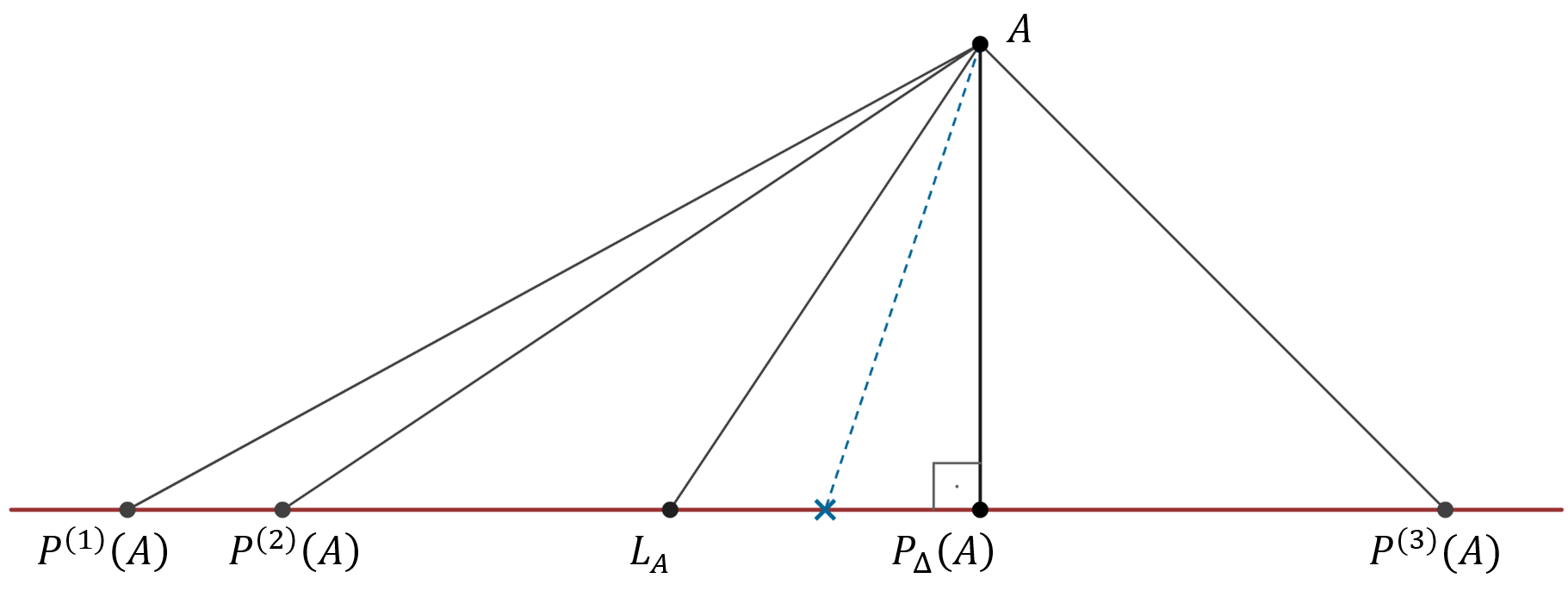
Figure 3: Situation described in reasoning by R.A.A.

That is, we have found $d$ matrices $Z_{i}=\lambda A_{i}+(1-\lambda)A_{i}^{*}$, $i=1,\dots,d$, such that

$$\left\|A-L_{A}\right\|=\left\|A-\sum_{i=1}^{d}\mathrm{id}_{[n_{i}]}\otimes A_{i}\right\|>\left\|A-\sum_{i=1}^{d}\mathrm{id}_{[n_{i}]}\otimes Z_{i}\right\|,$$

which is a contradiction with the definition of $L_{A}$.

The previous result allows us to describe the procedure to obtain the Laplacian approximation of a square matrix, in the form of an algorithm. We can visualize the complete algorithm in the form of pseudocode in Algorithm 2.

Algorithm 2 Laplacian decomposition Algorithm

1:procedure Lap($A^{*},\texttt{iter\_max},\texttt{tol}$)

2:     $A=A^{*}-(\mathrm{tr}(A)/N)\mathrm{id}_{N}$, $\texttt{iter}=1$, $\texttt{Lap}=0$

3:     while $\texttt{iter}<\texttt{iter\_max}$ do

4:         $A\leftarrow A-\texttt{Lap}$

5:         for $k=1,2,\ldots,d$ do

6:              $P_{k}(A)=\mathrm{id}_{n_{1}}\otimes\dots\otimes\mathrm{id}_{n_{k-1}}\otimes X_{k}\otimes\mathrm{id}_{n_{k+1}}\otimes\dots\otimes\mathrm{id}_{n_{d}}$

7:              $X_{k}\leftarrow\min_{X_{k}}\|A-\sum_{i=1}^{k}P_{i}(A)\|$

8:              $\texttt{Lap}=\texttt{Lap}+P_{k}(A)$

9:         end for

10:         if $\|A-\texttt{Lap}\|<\texttt{tol}$ then goto 14

11:         end if

12:         $\texttt{iter}=\texttt{iter}+1$

13:     end while

14:     return Lap

15:end procedure

4.1 Numerical Examples

4.1.1 Example 1: The adjacency matrix of a simple graph

First, let us show an example in which the projection $P_{\Delta}(A)$ coincides with $A$ and how the tensor representations is provided by the aforementioned proposed algorithm. Let us consider the simple graph $G(V,E)$, with $V=\{1,2,\ldots,6\}$ the set of nodes and $E=\{(1,4),(2,3),(2,5),(3,6),(5,6)\}$ the set of edges. Then, the adjacency matrix of $G$ is

$$A=\begin{pmatrix}0&1&0&1&0&0\\ 1&0&1&0&1&0\\ 0&1&0&0&0&1\\ 1&0&0&0&1&0\\ 0&1&0&1&0&1\\ 0&0&1&0&1&0\end{pmatrix}.$$

We want to find a Laplacian decomposition of the matrix $A\in{\mathbb{R}}^{6\times 6}$. Since $\mathrm{tr}(A)=0$, we can do this by following the iterative scheme given by Theorem 4.1. So, we look for $X_{1}\in{\mathbb{R}}^{2\times 2}$, $X_{2}\in{\mathbb{R}}^{3\times 3}$ matrices such that

$$P_{\Delta}(A)=X_{1}\otimes\mathrm{id}_{n_{2}}+\mathrm{id}_{n_{1}}\otimes X_{2},$$

where $n_{1}=2,n_{2}=3$. We proceed according to the algorithm:

1. Compute $X_{1}:$

   $$\min_{X_{1}}\|A-X_{1}\otimes\mathrm{id}_{n_{2}}\|\,\Rightarrow\,X_{1}=\begin{pmatrix}0&1\\ 1&0\end{pmatrix}.$$

2. Compute $X_{2}:$

   $$\begin{matrix}\begin{aligned} \min_{X_{2}}\|A-P_{1}(A)-\mathrm{id}_{n_{1}}\otimes X_{2}\|\,\Rightarrow\,X_{2}=\begin{pmatrix}0&1&0\\ 1&0&1\\ 0&1&0\end{pmatrix}.\end{aligned}\end{matrix}$$

Since the residual values is $||A-P_{\Delta}(A)||=0,$ the matrix $A\in\Delta$ and we can write it as

$$A=\begin{pmatrix}0&1\\ 1&0\end{pmatrix}\otimes\mathrm{id}_{n_{2}}+\mathrm{id}_{n_{1}}\otimes\begin{pmatrix}0&1&0\\ 1&0&1\\ 0&1&0\end{pmatrix}=P_{\Delta}(A).$$

4.1.2 Example 2: A bigger sparse matrix

Now, let us consider the following sparse matrix in $\mathrm{GL}({\mathbb{R}}^{30})$,

$$A=\left(\begin{array}[]{rrr|rrr}T_{1}&2I_{5}&-I_{5}&&&\\ 2I_{5}&T_{2}&2I_{5}&&I_{15}&\\ I_{5}&2I_{5}&T_{1}&&&\\ \hline\cr&&&T_{1}&2I_{5}&-I_{5}\\ &-I_{15}&&2I_{5}&T_{2}&2I_{5}\\ &&&I_{5}&2I_{5}&T_{1}\\ \end{array}\right),$$

where

$$T_{1}=\begin{pmatrix}[r]3&\phantom{-}2&\phantom{-}1&\phantom{-}0&-2\\ 2&3&2&1&0\\ 1&2&3&2&1\\ 0&1&2&3&2\\ -2&0&1&2&3\\ \end{pmatrix},\;T_{2}=\begin{pmatrix}[r]-1&2&1&0&-2\\ 2&-1&2&1&0\\ 1&2&-1&2&1\\ 0&1&2&-1&2\\ -2&0&1&2&-1\\ \end{pmatrix}$$

and $I_{k}$ es the identity matrix of size $k\times k$. We can visualize the matrix graphically with the Mathematica command MatrixPlot[A], In this case $\mathrm{tr}(A)=50\neq 0,$ so instead of looking for the Laplacian approximation of $A$, we will look for it of

$$\hat{A}=\left(A-\dfrac{\mathrm{tr}(A)}{30}\mathrm{id}_{30}\right),$$

which has null trace; see Figure 4.

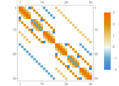
Figure 4: Representation of sparse matrix $A$ using Mathematica ¹⁹.

Again, we proceed according to the algorithm:

1. Compute $X_{1}:$

   $$\min_{X_{1}}\|\hat{A}-X_{1}\otimes\mathrm{id}_{n_{2}}\otimes\mathrm{id}_{n_{3}}\|\,\Rightarrow\,X_{1}=\begin{pmatrix}\phantom{-}0&1\\ -1&0\end{pmatrix}.$$

2. Compute $X_{2}:$

   $$\min_{X_{2}}\|\hat{A}-X_{1}\otimes\mathrm{id}_{n_{2}}\otimes\mathrm{id}_{n_{3}}-\mathrm{id}_{n_{1}}\otimes X_{2}\otimes\mathrm{id}_{n_{3}}\|\,\Rightarrow\,X_{2}=\begin{pmatrix}\frac{4}{3}&\phantom{-}2&-1\\ 2&-\frac{8}{3}&\phantom{-}2\\ 1&\phantom{-}2&\phantom{-}\frac{4}{3}\end{pmatrix}.$$

3. Compute $X_{3}:$

   $$\begin{matrix}\begin{aligned} \min_{X_{3}}\|\hat{A}-X_{1}\otimes\mathrm{id}_{n_{2}}\otimes\mathrm{id}_{n_{3}}-\mathrm{id}_{n_{1}}\otimes X_{2}\otimes\mathrm{id}_{n_{3}}-\mathrm{id}_{n_{1}}\otimes\mathrm{id}_{n_{2}}\otimes X_{3}\|\\ &\Rightarrow\,X_{3}=\begin{pmatrix}\phantom{-}0&\phantom{-}2&\phantom{-}1&\phantom{-}0&-2\\ \phantom{-}2&\phantom{-}0&\phantom{-}2&\phantom{-}1&\phantom{-}0\\ \phantom{-}1&\phantom{-}2&\phantom{-}0&\phantom{-}0&\phantom{-}2\\ \phantom{-}0&\phantom{-}1&\phantom{-}2&\phantom{-}0&\phantom{-}2\\ -2&\phantom{-}0&\phantom{-}1&\phantom{-}2&\phantom{-}0\end{pmatrix}.\end{aligned}\end{matrix}$$

The residue of the approximation of $\hat{A}$ is $\|\hat{A}-P_{\Delta}(\hat{A})\|=0,$ so, following Corollary 3.8, we can write the original matrix $A$ as

$$A=\dfrac{\mathrm{tr}(A)}{30}\mathrm{id}_{30}+X_{1}\otimes\mathrm{id}_{n_{2}}\otimes\mathrm{id}_{n_{3}}+\mathrm{id}_{n_{1}}\otimes X_{2}\otimes\mathrm{id}_{n_{3}}+\mathrm{id}_{n_{1}}\otimes\mathrm{id}_{n_{2}}\otimes X_{3}.$$

Note that the first term is

$$\dfrac{\mathrm{tr}(A)}{30}\mathrm{id}_{30}=\begin{pmatrix}\frac{5}{3}&0\\ 0&\frac{5}{3}\end{pmatrix}\otimes\mathrm{id}_{n_{2}}\otimes\mathrm{id}_{n_{3}},$$

and hence $A$ can be written as:

$$\begin{matrix}\begin{aligned} A=\begin{pmatrix}\frac{5}{3}&1\\ -1&\frac{5}{3}\end{pmatrix}\otimes\mathrm{id}_{n_{2}n_{3}}+\mathrm{id}_{n_{1}}\otimes\begin{pmatrix}\frac{4}{3}&\phantom{-}2&-1\\ 2&-\frac{8}{3}&\phantom{-}2\\ 1&\phantom{-}2&\phantom{-}\frac{4}{3}\end{pmatrix}\otimes\mathrm{id}_{n_{3}}+\mathrm{id}_{n_{1}n_{2}}\otimes\begin{pmatrix}\phantom{-}0&\phantom{-}2&\phantom{-}1&\phantom{-}0&-2\\ \phantom{-}2&\phantom{-}0&\phantom{-}2&\phantom{-}1&\phantom{-}0\\ \phantom{-}1&\phantom{-}2&\phantom{-}0&\phantom{-}0&\phantom{-}2\\ \phantom{-}0&\phantom{-}1&\phantom{-}2&\phantom{-}0&\phantom{-}2\\ -2&\phantom{-}0&\phantom{-}1&\phantom{-}2&\phantom{-}0\end{pmatrix}.\normalsize\end{aligned}\end{matrix}$$

5 Conclusions

We have presented a result to approximate a generic square matrix by its Laplacian form, and thus decompose it as the sum of two linearly independent matrices. This decomposition is motivated by the fact that tensor algorithms are more efficient when working with Laplacian matrices. We have also described the procedure to perform this approximation in the form of an algorithm and illustrated how it works on some basic examples.

With the proposed algorithm we may provide an alternative way to solve linear system $A\mathbf{x}=\mathbf{b}$. Due to its structure, this matrix decomposition can be interesting when studying sparse matrices, matrices that come from the discretization of a PDE, or adjacency matrices of simple graphs, among others. We will explore the computational gains of this approach in different contexts in forthcoming works.

References

• 1 Luzardo D, and Peña P AJ. Historia del Álgebra Lineal hasta los Albores del Siglo XX. Divulgaciones Matemáticas. 2006;14(2):153–170.
• 2 Saad Y. Iterative methods for linear systems of equations: A brief historical journey. In: Brenner SC, Shparlinski IE, Shu CW, and Szyld DB, editors. 75 Years of Mathematics of Computation. vol. 754 of Contemporary Mathematics. American Mathematical Society; 2020. .
• 3 Saad Y, and Van der Vorst HA. Iterative solution of linear systems in the 20th century. Journal of Computational and Applied Mathematics. 2000;123(1):1–33.
• 4 Leiserson CE, Rivest RL, Cormen TH, and Stein C. Introduction to algorithms;.
• 5 Strang G. Linear algebra and its applications. Belmont, CA: Thomson, Brooks/Cole; 2006.
• 6 Golub GH, and Van Loan CF. Matrix computations. JHU press; 2013.
• 7 Nouy A. Chapter 4: Low-Rank Methods for High-Dimensional Approximation and Model Order Reduction. In: Model Reduction and Approximation. Society for Industrial and Applied Mathematics; 2017. p. 171–226.
• 8 Hackbusch W. Tensor Spaces and Numerical Tensor Calculus (Second Edition). Springer Series in Computational Mathematics. Springer Cham; 2019.
• 9 Simoncini V. Numerical solution of a class of third order tensor linear equations. Boll Unione Mat Ital. 2020;13:429–439.
• 10 Ammar A, Chinesta F, and Falcó A. On the convergence of a Greedy Rank-One Update algorithm for a class of linear systems. Arch Comput Methods Eng. 2010;17(4):473–486.
• 11 Georgieva I, and Hofreither C. Greedy low-rank approximation in Tucker format of solutions of tensor linear systems. J Comput Appl Math. 2019;358:206–220.
• 12 Falcó A, and Nouy A. Proper generalized decomposition for nonlinear convex problems in tensor Banach spaces. Numer Math. 2012;121:503–530.
• 13 Quesada C, Xu G, González D, Alfaro I, Leygue A, Visonneau M, et al. Un método de descomposición propia generalizada para operadores diferenciales de alto orden. Rev Int Metod Numer. 2015;31(3):188–197.
• 14 Falcó A. Tensor Formats Based on Subspaces are Positively Invariant Sets for Laplacian-Like Dynamical Systems. In: Numerical Mathematics and Advanced Applications ENUMATH 2013. Lecture Notes in Computational Science and Engineering;. .
• 15 Falcó A, Hackbusch W, and Nouy A. On the Dirac–Frenkel Variational Principle on Tensor Banach Spaces. Foundations of Computational Mathematics. 2018;19(1):159–204.
• 16 Hackbusch W, Khoromskij B, Sauter S, and Tyrtyshnikov E. Use of tensor formats in elliptic eigenvalue problems. Numer Lin Algebra Appl. 2012;19:133–151.
• 17 Heidel G, Khoromskaia V, Khoromskij BN, and Schulz V. Tensor product method for fast solution of optimal control problems with fractional multidimensional Laplacian in constraints. J Comput Phys. 2021;424:109865.
• 18 Gallier J, and Quaintance J. Differential Geometry and Lie Groups. Springer International Publishing; 2020. Available from: https://doi.org/10.1007/978-3-030-46040-2.
• 19 Inc WR. Mathematica, Version 13.1. Champaign, IL, 2022;. Available from: https://www.wolfram.com/mathematica.