An Iterative 5G Positioning and Synchronization Algorithm in NLOS Environments with Multi-Bounce Paths

Abstract

5G positioning is a very promising area that presents many opportunities and challenges. Many existing techniques rely on multiple anchor nodes and line-of-sight (LOS) paths, or single reference node and single-bounce non-LOS (NLOS) paths. However, in dense multipath environments, identifying the LOS or single-bounce assumptions is challenging. The multi-bounce paths will make the positioning accuracy deteriorate significantly. We propose a robust 5G positioning algorithm in NLOS multipath environments. The corresponding positioning problem is formulated as an iterative and weighted least squares problem, and different weights are utilized to mitigate the effects of multi-bounce paths. Numerical simulations are carried out to evaluate the performance of the proposed algorithm. Compared with the benchmark positioning algorithms only using the single-bounce paths, similar positioning accuracy is achieved for the proposed algorithm.

I Introduction

5G New Radio offers great opportunities for accurate localization by introducing large bandwidth, high carrier frequency, and large antenna array. Most of the state-of-the-art localization techniques are designed based on multiple anchor nodes and line-of-sight (LOS) paths, or single reference node and single bounce non-LOS (NLOS) paths radio propagation [1]. A low complexity, search-free 5G mmWave localization and mapping method that is able to operate using single-bounce diffuse multipath is proposed in [2], where LOS and specular multipath are not required. In [3], the authors propose a localization algorithm for use in NLOS environments. The single bounce scattering model is utilized to model the NLOS propagation and to estimate the position of a mobile station when the observations are the time-difference-of-arrival (TDOA), the angle-of-departure (AOD), and the angle-of-arrival (AOA). The proposed algorithm uses the underlying geometry of the radio propagation paths to estimate the position of the mobile station. Paper [4] focuses on indoor scenarios which are multipath and rich scattering environments considering NLOS propagation. Based on the measured AOD, AOA, and time-of-arrival (TOA), a three dimensional (3D) least squares (LS) positioning algorithm is proposed assuming a single-bounce reflection in each NLOS propagation path.

However, for 5G positioning in dense multipath environments, the LOS or single bounce assumptions can be invalid. The multi-bounce paths will make the positioning accuracy deteriorate significantly. One option is to remove paths directly based on geometric grounds if they are not LOS or single-bounce, using the angle difference between the LOS path and a possible multi-bounce path [5]. Because the channel gains for the multiple-bounce paths are much smaller than that of the LOS and single-bounce NLOS paths, a part of previous research ignores the multi-bounce paths or just uses received power to identify these multi-bounce paths [6]. However, the results in [7] show that it could be difficult to distinguish the single-bounce and double-bounce paths from the multi-bounce paths by using the received power only. Furthermore, the study in [8] indicates that some specific spatial shape and the material of surface will also influence the identification. It is shown in [9] that multi-bounce paths should be considered in real environment because the power and the total number of multi-bounce paths occupy a large proportion.

In this paper, we investigate robust positioning techniques to relief these LOS and single-bounce assumptions using the available channel parameter measurements, such as AOD, AOA, TOA, and channel gain [10]. The main contributions are summarized as follows:

• A weighted least square (WLS) based robust 5G positioning and synchronization algorithm based on single BS in NLOS multipath environment is proposed. In the proposed WLS-based algorithm, different weights are utilized to mitigate the effects of multiple bounce paths.

• Based on the generalized likelihood ratio test (GLRT) method, we propose an iterative strategy to distinguish single-bounce and multi-bounce paths.

• A numerical study on the distribution of the measurement errors is conducted, which demonstrates that the proposed algorithm achieves robust localization performance.

II Problem Formulation

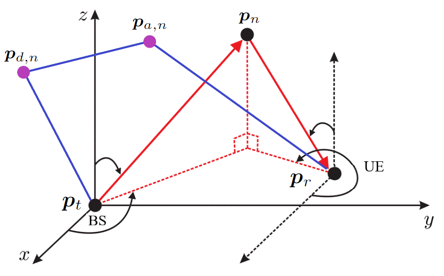
Figure 1: System model with single-bounce and multiple-bounce NLOS propagation paths, the user equipment “UE”, the base station “BS”, and the incidence points $\bm{p}_{d,n}$ and $\bm{p}_{a,n}$ for multiple bounce paths, $\bm{p}_{n}=\bm{p}_{d,n}=\bm{p}_{a,n}$ for single bounce paths. For the LOS path, we introduce $\bm{p}_{0}$ as any point on the line segment strictly excluding $\bm{p}_{\rm{t}}$ and $\bm{p}_{\rm{r}}$.

We consider a down-link 3D positioning scenario with a single base station (BS) with known location $\bm{p}_{t}=[x_{t},y_{t},z_{t}]^{\mathsf{T}}$ and single user equipment (UE) with unknown location $\bm{p}_{r}=[x_{r},y_{r},z_{r}]^{\mathsf{T}}$ and clock bias $\tau_{B}$. We assume that the orientation between BS and UE is known. As shown in Fig. 1, the complex propagation environment leads to single-bounce NLOS paths (show in red) and multi-bounds NLOS paths (shown in blue), in addition to a possible LOS path (not shown).

Based on a channel parameter estimation method, we obtain, for each path $n$, estimates of the channel gain (amplitude) $\gamma_{n}\geq 0$, the azimuth and elevation angles of AOD, denoted by $(\phi_{d,n},\theta_{d,n})$; the azimuth and elevation angles of AOA, denoted by $(\phi_{a,n},\theta_{a,n})$, the TOA $\tau_{n}=d_{n}/c+\tau_{B}$, where $d_{n}$ is the total propagation distance, $c$ is the speed of light, and $\tau_{B}$ is the unknown clock bias caused by imperfect synchronization between BS and UE. For each path, it is unknown whether it is LOS, single-bounce, or multiple-bounce.

We make use of the following essential geometric relations, which hold for LOS and single-/double-bounce paths, but not for multi-bounce paths larger than two [2]:

$$d_{n} =\|\bm{p}_{d,n}-\bm{p}_{t}\|+\|\bm{p}_{a,n}-\bm{p}_{d,n}\|+\|\bm{p}_{a,n}-\bm{p}_{r}\|$$ (1a)

$$\phi_{a,n} =\pi+\mathrm{atan}2\left(y_{a,n}-y_{r},x_{a,n}-x_{r}\right)$$ (1b)

$$\theta_{a,n} =\mathrm{asin}\left(\frac{z_{a,n}-z_{r}}{\|\bm{p}_{a,n}-\bm{p}_{r}\|}\right)$$ (1c)

$$\phi_{d,n} =\mathrm{atan}2\left(y_{d,n}-y_{t},x_{d,n}-x_{t}\right)$$ (1d)

$$\theta_{d,n} =\mathrm{asin}\left(\frac{z_{d,n}-z_{t}}{\|\bm{p}_{d,n}-\bm{p}_{t}\|}\right).$$ (1e)

where $\|\cdot\|$ is Euclidean norm. Our goal is to estimate the UE location $\bm{p}_{r}$, based on the estimated channel parameters. We tackle the problem based on the methods from [2].

III Proposed Method

In order to solve the positioning problem, we first establish identities that hold for each path $n$, be it LOS, single-bounce, or multi-bounce. Then we describe a method that can estimate the UE position and clock bias from at least 2 multipath channel parameter estimates (the 2 multipath should be either LOS or single-bounce paths). Finally, we use both these results to propose our final method, which involves using a set of ordered paths, combined with change detection in the positioning residuals.

III-A Identities for 5G Positioning and Synchronization

Before describing the proposed method, we first list identities valid for any path $n$, be it LOS, single-bounce, or multi-bounce. We first define

$$\bm{f}_{t,n}=\begin{bmatrix}\cos(\hat{\theta}_{d,n})\cos(\hat{\phi}_{d,n})\\ \cos(\hat{\theta}_{d,n})\sin(\hat{\phi}_{d,n})\\ \sin(\hat{\theta}_{d,n})\end{bmatrix},$$ (2)

which points along the AOD of path $n\in\{1,2,\ldots,{N}\}$; and $\mathbf{f}_{r,n}$ is defined equivalently for the AOA, pointing from the UE towards the $n$-th artificial specular point $\bm{p}_{a,n}$:

$$\bm{f}_{r,n}=\begin{bmatrix}\cos(\hat{\theta}_{a,n})\cos(\hat{\phi}_{a,n})\\ \cos(\hat{\theta}_{a,n})\sin(\hat{\phi}_{a,n})\\ \sin(-\hat{\theta}_{a,n}).\end{bmatrix}.$$ (3)

Then, we have the following relations, valid for double bounce, single bounce and direct paths:

$$\left\{\begin{aligned} \bm{p}_{d,n}&=\bm{p}_{t}+\xi_{d,n}d_{n}\bm{f}_{t,n}\\ \bm{p}_{a,n}&=\bm{p}_{r}+\xi_{a,n}d_{n}\bm{f}_{r,n}\\ \xi_{d,n}&+\xi_{a,n}\leq 1,\text{ and }0<\xi_{d,n},\xi_{a,n}<1\end{aligned}\right.$$ (4)

where $\xi_{d,n}$ and $\xi_{a,n}$ are unknown and represent the fraction of the delay $\hat{\tau}_{n}$ that is attributed to the line from BS to the first scatter point $\bm{p}_{d,n}$ and from UE to the second scatter point $\bm{p}_{a,n}$. Note that of $\xi_{d,n}+\xi_{a,n}=1,\text{ and }0<\xi_{d,n},\xi_{a,n}<1$ for single bounce paths and the LOS path. We now introduce $\bm{e}_{n}=\bm{p}_{d,n}-\bm{p}_{a,n}$, then we can express (4) as

$$\bm{p}_{r}=\bm{p}_{t}+\mathbf{e}_{n}+\left(\xi_{d,n}\mathbf{q}_{t,n}-\xi_{a,n}\mathbf{q}_{r,n}\right),\forall n$$ (5)

where $\mathbf{q}_{t,n}=d_{n}\bm{f}_{t,n}$ and $\mathbf{q}_{r,n}=d_{n}\bm{f}_{r,n}$. For multi-bounce paths, we have $\|\bm{e}_{n}\|_{2}>0$. Because $\mathbf{e}_{n}$ is a unknown variable, the range of the feasible solutions for (5) is unbounded. Therefore, it is challenging to estimate the UE position by solving a set of linear equations using WLS methods.

III-B WLS-based 5G Positioning and Synchronization

For LOS and single-bounce cases, we have $\mathbf{e}_{n}=\mathbf{0}$, and $\xi_{a,n}=1-\xi_{d,n}$, then (5) can be simplified as

$$\bm{p}_{r}=\bm{p}_{t}+\xi_{d,n}\mathbf{q}_{t,n}-(1-\xi_{d,n})\mathbf{q}_{r,n},$$ (6)

The UE position can be determined if there are multiple single-bounce paths. Specifically, from (6), we establish

$$\bm{p}_{r} =\bm{p}_{t}+c\left(\hat{\tau}_{n}-\tau_{B}\right)\xi_{d,n}\bm{f}_{t,n}-c\left(\hat{\tau}_{n}-\tau_{B}\right)\left(1-\xi_{d,n}\right)\bm{f}_{r,n}$$

$$=\bm{p}_{t}-c\hat{\tau}_{n}\bm{f}_{r,n}+c\tau_{B}\bm{f}_{r,n}+c\xi_{d,n}\left(\hat{\tau}_{n}-\tau_{B}\right)\left(\bm{f}_{t,n}+\bm{f}_{r,n}\right)$$

$$={\bm{\delta}}_{n}+c\tau_{B}\bm{f}_{r,n}+{\xi}_{d,n}{\bm{u}}_{n}-c\tau_{B}{\xi}_{d,n}\left(\bm{f}_{t,n}+\bm{f}_{r,n}\right),$$ (7)

where ${\bm{\delta}}_{n}=\bm{p}_{t}-c\hat{\tau}_{n}\bm{f}_{r,n}$, ${\bm{u}}_{n}=c\hat{\tau}_{n}\left(\bm{f}_{t,n}+\bm{f}_{r,n}\right)$, ${\bm{v}}_{n}=c\left(\bm{f}_{t,n}+\bm{f}_{r,n}\right)$, and $\tau_{\xi,n}=\tau_{B}{\xi}_{d,n}$. We further rewrite (7) as

$$\begin{bmatrix}\bm{I}_{3}&-\bm{u}_{n}&-c\bm{f}_{r,n}&\bm{v}_{n}\end{bmatrix}\begin{bmatrix}\bm{p}_{r}\\ {\xi}_{d,n}\\ \tau_{B}\\ \tau_{\xi,n}\end{bmatrix}=\bm{\delta}_{n}.$$ (8)

With the estimations of $N$ sets of multipath channel parameters, we can establish $3N$ linear equations with $(4$+$2N)$ unknowns $\bm{\mu}=\begin{bmatrix}\bm{p}^{\mathrm{T}}_{r},\,{\xi}_{d,1},\,\cdots,\,{\xi}_{d,N},\,\tau_{B},\tau_{\xi,1},\cdots,\tau_{\xi,N}\end{bmatrix}^{\mathrm{T}}$. Therefore, with $N\geq 2$ multipath components, we have

$$\bm{U}\bm{\mu}=\bm{\delta}$$ (9)

where $\bm{\delta}=\begin{bmatrix}\bm{\delta}_{1}^{\mathrm{T}},&\bm{\delta}_{2}^{\mathrm{T}},&\cdots&\bm{\delta}_{N}^{\mathrm{T}}\end{bmatrix}^{\mathrm{T}}\in\mathbb{R}^{3N\times 1}$ and $\bm{U}\in\mathbb{C}^{3N\times(2N+4)}$ is defined as

$$\bm{U}=\left[\begin{array}[]{cccccccc}\bm{I}_{3}&-\bm{u}_{1}&&\bm{0}&-c\bm{f}_{r,1}&\bm{v}_{1}&&\bm{0}\\ \vdots&&\ddots&&\vdots&&\ddots&\\ \bm{I}_{3}&\bm{0}&&-\bm{u}_{N}&-c\bm{f}_{r,1}&\bm{0}&&\bm{v}_{N}\end{array}\right].$$ (10)

The variable ${\bm{\mu}}$ can be estimated with a weighted least-square solution as

$$\hat{\bm{\mu}} =\left(\bm{U}^{\mathrm{H}}\mathbf{W}\bm{U}\right)^{-1}\bm{U}^{\mathrm{H}}\mathbf{W}\bm{\delta},$$ (11)

where the block diagonal matrix

$$\mathbf{W}=\text{blkdiag}\big{[}w_{1}\bm{I}_{3},\,w_{2}\bm{I}_{3},\cdots,w_{N}\bm{I}_{3}\big{]}\in\mathbb{R}^{3N\times 3N},$$

accounts for the normalized weight of each path, via $w_{n}=\gamma_{n}/(\sum_{n}\gamma_{n}).$ Note that $\mathbf{W}=\bm{I}_{3N}$ is the conventional LS solution. Finally, the estimated UE position is $\hat{\bm{p}}_{r}=\hat{\bm{{\mu}}}_{[1:3]}$

III-C WLS with Change Detection

We first order the paths, e.g., based on delay (from smallest to largest), or based on amplitude (from largest to smallest). Generally speaking, the first two arrival paths are usually LOS or single-bounce paths, because most multi-bounce paths have larger TOA. We thus use the first $k=2$ paths in (11) to determine an initial estimate, say $\bm{p}_{r}^{(1)}$. Similarly, we compute $\bm{p}_{r}^{(t)}$ from the first $k+t-1$ paths, $t=2,3,\ldots$, using (11).

TABLE I: Relative UE estimation error using different number of the first coming paths.

Step $t$	Number of paths	Estimated $\bm{p}_{r}$	Relative estimation error
1	2	$\bm{p}_{r}^{(1)}$	0
2	3	$\bm{p}_{r}^{(2)}$	$\Delta_{1}=\|\bm{p}_{r}^{(2)}-\bm{p}_{r}^{(1)}\|$
3	4	$\bm{p}_{r}^{(3)}$	$\Delta_{2}=\|\bm{p}_{r}^{(3)}-\bm{p}_{r}^{(1)}\|$
4	5	$\bm{p}_{r}^{(4)}$	$\Delta_{3}=\|\bm{p}_{r}^{(4)}-\bm{p}_{r}^{(1)}\|$

From these estimates, we compute the instant relative estimation error,

$$\Delta_{t}=\|\bm{p}_{r}^{(t)}-\bm{p}_{r}^{(1)}\|,$$ (12)

and constructing the following positioning residual vector (see also Table I)

$$\bm{\Delta}^{(t)}=\begin{bmatrix}\Delta_{1}&\Delta_{2}&\cdots&\Delta_{t}\end{bmatrix}^{\mathrm{T}}.$$ (13)

From (5), we recall that for multi-bounce paths, $\|\bm{e}_{n}\|>0$,

Figure 2: Motivation of using the slope change detection method to selected the single bounce paths. The first 3 paths are single-bounce paths, while the multiple bounce paths appear starting from path 4.

so that for the proposed estimator in (11), as shown in Fig. 2, we expect a larger relative UE estimation error $\Delta_{t}$ when a multi-bounce path is included for WLS estimation. Since paths later in the ordering are more likely to be multi-bounce, we can interpret this as a single-sensor change detection problem with observations $\bm{\Delta}^{(t)}$.

III-C1 Change Point Detection

Change point detection is an active research area in statistics due to its importance across a wide range of applications. The change-point can be modeled as a shift in the means of the observations, which is good for modeling an abrupt change [11]. However, in many applications, the change point may cause a gradual change to the observations, which can be well approximated by a slope change in the means of the observations [12]. Under the hypothesis of no change, the observations are drawn from $\mathcal{N}\left(\mu,\sigma^{2}\right)$, i.e., with a fixed mean $\mu$ and variance $\sigma^{2}$. When a change occurs at $\kappa$ (the unknown change-point), then the mean of the observations changes linearly from the change-point time $\kappa+1$, which is given by $\mu+s(t-\kappa)$ for all $t>\kappa$, and the variance remains $\sigma^{2}$. Here, the unknown rate of change is $s\neq 0$. The above setting can formulate as the following hypothesis testing problem:

$$\mathcal{H}_{0}: \Delta_{i}\sim\mathcal{N}\left(\mu,\sigma^{2}\right),i\geq 1$$ (14)

$$\mathcal{H}_{1}: \Delta_{i}\sim\begin{cases}\mathcal{N}\left(\mu,\sigma^{2}\right)&i\leq\kappa\\ \mathcal{N}\left(\mu+s(i-\kappa),\sigma^{2}\right)&i>\kappa.\end{cases}$$

Our goal is now to establish a detection rule that detects as soon as possible after a change-point occurs and avoid raising false alarms when there is no change. It can be solved efficiently by generalized likelihood ratio test (GLRT) method [13]. Since the observations are independent, for an assumed change-point location $\kappa=k$, the log-likelihood for observations up to time $t>k$ is given by [12]

$$\ell_{k,t,s}=\frac{1}{2\sigma^{2}}\sum_{i=k+1}^{t}\left[2s\left(\Delta_{i}-\mu\right)(i-k)-s^{2}(i-k)^{2}\right].$$ (15)

The unknown rate-of-change $s$ can be replaced by its maximum likelihood estimator. Given the current number of observations $t$ and a assumed change-point location $k$, by setting the derivative of the log-likelihood function (15) to 0, we have [12]

$$\hat{s}_{k,t}=\frac{\sum_{i=k+1}^{t}(i-k)\left(\Delta_{i}-\mu\right)}{\sum_{i=k+1}^{t}(i-k)^{2}}.$$ (16)

Let $\tau=t-k$ be the number of samples after the change-point $k$ and $U_{k,t}=\left(A_{\tau}\right)^{-1/2}W_{k,t}$, where $A_{\tau}=\sum_{i=1}^{\tau}i^{2}$ and $W_{k,t}=\sum_{i=k+1}^{t}(i-k)\left(\Delta_{i}-\mu\right)/\sigma_{n}$. Substitution of (16) into (15), we obtain the following GLRT procedure

$$t^{*}=\inf\left\{t:\max_{0\leq k<t}\left[U_{k,t}^{2}/2\right]\geq h\right\},$$ (17)

where $h$ is a prescribed threshold. Since distribution of $\Delta_{i}$ under $\mathcal{H}_{o}$ is known or can be estimated from the measure, $h$ can be chosen based on the desired false alarm probability.

III-C2 Final Method

At each iteration $t$, the slope change detection technique introduced in Section III-C, is utilized on $\bm{\Delta}^{(t)}$ to find the first abrupt change. Stop until the first abrupt change point is detected or reaching the maximum iteration number $N-1$. The proposed algorithm is summarized in Algorithm 1.

Algorithm 1 5G Positioning and Synchronization Algorithm

1:$N\geq 2$ sets of channel parameters ($\tau_{j}<\tau_{j+1}$)

2:if $N=2$ then

3:     Estimate $\bm{p}_{r}$ from the $k=2$ paths using (11).

4:else

5:     for $t=1$ do

6:         Estimate $\bm{\mu}_{r}^{(1)}$ from the first $k=2$ paths by (11).

7:     end for

8:     $t=t+1$

9:     Estimate $\bm{\mu}_{r}^{(t)}$ from the first $k+t-1$ paths by (11).

10:     Compute $\Delta_{t}$ using (12).

11:     Construct $\bm{\Delta}^{(t)}$ using (13)

12:     Estimate $t^{*}$ using (17).

13:     if $\exists t^{*}$ then

14:         Estimate $\bm{p}_{r}$ using the selected $t^{*}$ paths.

15:     else

16:         Estimate $\bm{p}_{r}$ using all the paths.

17:     end if

18:end if

IV Numerical Results

In this section, we evaluate the performance of the proposed method based on realistic ray-tracing data.

IV-A Simulation Scenario

In the following simulations, 3D Wireless Prediction Software Wireless InSite is utilized to generate the channel measurements. It is a suite of ray-tracing models and high-fidelity EM solvers for the analysis of site-specific radio wave propagation and wireless communication systems. The BS is located at $\bm{p}_{t}=[621,447,30]^{\mathrm{T}}$, and 10 different UE positions are considered, for the $i$th UE position

$$\bm{p}_{r_{i}}=[600,499+i,1.5]^{\mathrm{T}},\text{ where }i=1,2,\cdots,10.$$ (18)

The clock bias is set to $\tau_{B}=330$ ns. Gaussian noises are added on the path parameters, $\mathcal{N}(0,\sigma_{a})$ for AOA and AOD measurements, and $\mathcal{N}(0,\sigma_{r})$ for TOA measurements. As shown in Fig. 3, a complex urban and mixed path environment is considered. Based on this environment, the ray-tracer determines all feasible propagation paths and returns their channel gain $\gamma_{n}\geq,0$, AOD $(\phi_{d,n},\theta_{d,n})$, AOA $(\phi_{a,n},\theta_{a,n})$, and propagation distance $d_{n}$. Different levels of measurement error are added, as will be explained shortly.

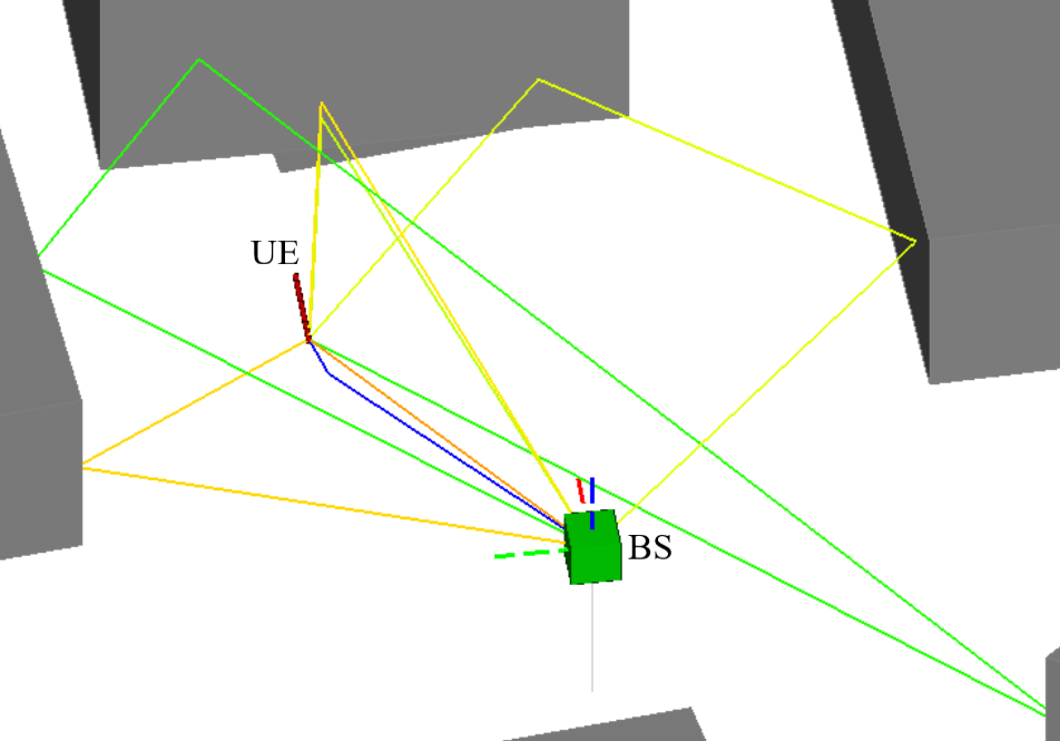
Figure 3: Wireless Insite simulation setup, including the BS, the UE and several objects, which reflect and scatter the signal.

The performance of the method is evaluated in terms of two performance metrics: positioning root-mean-square error (RMSE) (19) and clock bias RMSE (20), which are given by

$$\text{RMSE}_{\bm{p}_{r}} =\sqrt{\frac{\sum_{k=1}^{K}\|\hat{\bm{p}}_{r,k}-\bm{p}_{r}\|}{K}},$$ (19)

$$\text{RMSE}_{\tau_{B}} =\sqrt{\frac{\sum_{k=1}^{K}\|\hat{\tau}_{B_{k}}-\tau_{B}\|}{K}},$$ (20)

where $K=500$ is the number of independent runs, $\hat{\bm{p}}_{r,k}$ and $\hat{\tau}_{B_{k}}$ are the estimated UE position and clock bias for the $k$th trial, respectively. As a benchmark, the proposed method is compared with using all the paths (which we expect will degrade performance) and only using the single bounce paths (which is an optimistic performance bound).

IV-B Results and Discussion

Fig. 4 shows, for each UE position, the amplitude of the paths as a function of delay for the different UE locations. LOS, single and multiple bounce paths are observable as shown by the different colors. We observe that LOS paths arrive first and have largest power. Generally single-bounce paths arrive before multi-bounce paths and have a larger power. However, there are cases where multi-bounce paths arrive with greater power than single-bounce paths.

Figure 4: The path information obtained from Wireless Insite software for 10 different scenarios.

Figure 5: Gaussian noise $\mathcal{N}(0,\sigma_{a})$ is added on the AOA, AOD measurements, and $\mathcal{N}(0,\sigma_{r})$ is added on TOA measurements.

Figure 6: Gaussian noise $\mathcal{N}(0,\sigma_{a})$ is added on the AOA, AOD measurements, and $\mathcal{N}(0,\sigma_{r})$ is added on TOA measurements.

The performance is evaluated by considering 10 different scenarios as shown in Fig. 4, as well as considering different AOA, AOD and TOA measurement errors. The positioning and synchronization performance is shown in Fig. 5 and Fig. 6, respectively, as a function of the AOA and AOD error standard deviation, for different levels of TOA standard deviation (expressed in meters). It can be observed that sub-meter accuracy is achievable when the angle error standard deviation is small (below 0.01 rad) and the TOA error standard deviation is around 0.1 m. The proposed method performs robustly, even in the presence of multi-bounce paths, attaining the performance of using only single bounce paths. With the increase of AOA and AOD measurement errors, positioning RMSE of all methods increase, but is still better than that of using all paths. This shows that the proposed method can distinguish single- and multi-bounce paths in multipath environments and can control errors to a small level. In terms of clock bias estimation performance, similar conclusions can be drawn.

V Conclusion

We propose a robust algorithm to mitigate the effect of multi-bounce paths, based on a combination of weighted least squares and a change detection approach. Numerical results are provided to evaluate the performance of the algorithm, and the results show that it can greatly improve the positioning accuracy. One of the assumptions we made is that the first two arrival paths are single bounce paths, which may not always be true. In future work, we will further improve the applicability of the algorithm as well as the localization accuracy.

References

- [1] Z. Xiao and Y. Zheng, “An overview on integrated localization and communication towards 6G,” Science China Information Sciences, vol. 65, no. 131301, pp. 1–46, 2021.
- [2] F. Wen and H. Wymeersch, “5G synchronization, positioning, and mapping from diffuse multipath,” IEEE Wireless Communications Letters, vol. 10, no. 1, pp. 43–47, 2021.
- [3] B. Y. Shikur and T. Weber, “TDOA/AOD/AOA localization in NLOS environments,” in 2014 IEEE International Conference on Acoustics, Speech and Signal Processing (ICASSP), 2014, pp. 6518–6522.
- [4] X. Wei, N. Palleit, and T. Weber, “AOD/AOA/TOA-based 3D positioning in NLOS multipath environments,” in IEEE 22nd International Symposium on Personal, Indoor and Mobile Radio Communications (PIMRC), 2011, pp. 1289–1293.
- [5] A. Kakkavas, H. Wymeersch, G. Seco-Granados, M. H. Castañeda García, R. A. Stirling-Gallacher, and J. A. Nossek, “Power allocation and parameter estimation for multipath-based 5G positioning,” IEEE Transactions on Wireless Communications, pp. 1–1, 2021.
- [6] K. Mao, Q. Zhu, M. Song, B. Ning, B. Hua, W. Zhong, and X. Chen, “A novel non-stationary channel model for UAV-to-vehicle mmWave beam communications,” in International Conference on Machine Learning and Intelligent Communications. Springer, 2020, pp. 471–484.
- [7] S.-W. Ko, H. Chae, K. Han, S. Lee, D.-W. Seo, and K. Huang, “V2X-based vehicular positioning: Opportunities, challenges, and future directions,” IEEE Wireless Communications, vol. 28, no. 2, pp. 144–151, 2021.
- [8] Y. Geng, D. Shrestha, V. Yajnanarayana, E. Dahlman, and A. Behravan, “Joint scatterer localization and material identification using radio access technology,” arXiv preprint arXiv:2110.03880, 2021.
- [9] P. Koivumäki, A. Karttunen, and K. Haneda, “Wave scatterer localization in outdoor-to-indoor channels at 4 and 14 GHz,” in 2022 16th European Conference on Antennas and Propagation (EuCAP), 2022, pp. 1–5.
- [10] Y. Ge, F. Wen, H. Kim, M. Zhu, F. Jiang, S. Kim, L. Svensson, and H. Wymeersch, “5G SLAM using the clustering and assignment approach with diffuse multipath,” Sensors, vol. 20, no. 16, 2020.
- [11] R. Killick, P. Fearnhead, and I. A. Eckley, “Optimal detection of changepoints with a linear computational cost,” Journal of the American Statistical Association, vol. 107, no. 500, pp. 1590–1598, 2012.
- [12] Y. Cao, Y. Xie, and N. Gebraeel, “Multi-sensor slope change detection,” Annals of Operations Research, vol. 263, no. 1, pp. 163–189, 2018.
- [13] O. Besson, A. Coluccia, E. Chaumette, G. Ricci, and F. Vincent, “Generalized likelihood ratio test for detection of Gaussian rank-one signals in Gaussian noise with unknown statistics,” IEEE Transactions on Signal Processing, vol. 65, no. 4, pp. 1082–1092, 2017.