Periodic potential can enormously boost
free particle transport induced by active fluctuations

Abstract

Active fluctuations are detected in a growing number of systems due to self-propulsion mechanisms or collisions with active environment. They drive the system far from equilibrium and can induce phenomena which at equilibrium states are forbidden by e.g. fluctuation-dissipation relations and detailed balance symmetry. Understanding of their role in living matter is emerging as a challenge for physics. Here we demonstrate a paradoxical effect in which a free particle transport induced by active fluctuations can be boosted by many orders of magnitude when the particle is additionally subjected to a periodic potential. In contrast, within the realm of only thermal fluctuations the velocity of a free particle exposed to a bias is reduced when the periodic potential is switched on. The presented mechanism is significant for understanding nonequilibrium environments such as living cells where it can explain from a fundamental point of view why spatially periodic structures known as microtubules are necessary to generate impressively effective intracellular transport. Our findings can be readily corroborated experimentally e.g. in a setup comprising a colloidal particle in an optically generated periodic potential.

Microscopic systems are inherently immersed in a sea of thermal fluctuations that may strongly influence their properties or even induce an entirely new phenomenology. Celebrated examples include stochastic benzi1981 ; gammaitoni1998 or coherence pikovsky1997 ; lindner2004 resonance, anomalous diffusion bouchaud1990 ; metzler2014 ; spiechowicz2019njp , ratchet effects hanggi2009 ; reichhardt2017 ; spiechowicz2016scirep , negative mobility machura2007 ; nagel2008 ; slapik2019 or thermal noise induced dynamical localization spiechowicz2017scirep ; spiechowicz2019chaos , to name only a few. Nevertheless impact of thermal equilibrium fluctuations is limited by fundamental laws of nature such as the fluctuation-dissipation theorem kubo1966 ; marconi2008 or the detailed balance symmetry cates2012 ; gnesotto2018 .

These restrictions are no longer true for a nonequilibrium environment which keeps the system permanently out of thermal equilibrium even in the absence of external perturbations. A prototypical example are active fluctuations manifesting themselves either in (i) active matter harvesting energy from the environment into a self-propulsion drive ramaswamy2010 ; romanczuk2012 ; cates2012 ; marchetti2013 ; bechinger2016 ; reichhardt2017 or (ii) active bath such as a suspension of active colloids or swimming microorganisms (e.g. bacteria Escherichia coli) pushing around a passive system bechinger2016 ; maggi2014 ; kanazawa2015 ; maggi2017 ; dabelow2019 . Their relevance in biological systems is emerging as a hot topic which is in the focus of researchers across all branches of natural science kanazawa2020 . For instance, the latest breaking experimental results make it clear that active fluctuations in living cells, generated by using energy derived from metabolic activities, are not just noise but are utilized to promote various physiological processes. In particular, biological motors such as kinesin or dynein benefit from active fluctuations and enhance their directional movement ezber2020 ; ariga2021 .

Within the realm of thermal equilibrium fluctuations the directed velocity of a free particle exposed to a bias is usually reduced or at best conserved when an additional periodic potential is switched on risken . Similarly, the diffusion coefficient $D_{0}$ of the free Brownian particle subjected to a periodic force is reduced to its effective diffusion constant $D<D_{0}$ lifson . In this Letter we demonstrate an opposite striking case: the particle can harness active nonequilibrium fluctuations to exploit an unbiased periodic potential and enhance its directed velocity much larger than for free transport. We identify its origin in smart nature of active fluctuations which unlike thermal ones are not constrained by the equilibrium state and therefore may optimize themselves to make use of a periodic potential.

Our results are significant for understanding nonequilibrium environments and addressing important theoretical questions concerning thermodynamics of active systems such as molecular motors inside living cells. They can be corroborated experimentally in a setup comprising a colloidal particle in an optically generated periodic potential park2020 ; paneru2021 or tested for real biological motors ezber2020 ; ariga2021 . Moreover, they may open new avenues for designing ultrafast and efficient micro and nanoscale machines.

We start our considerations with overdamped motion of a free particle subjected to both active nonequilibrium fluctuations $\eta(t)$ and thermal noise $\xi(t)$,

$$\dot{x}=\eta(t)+\sqrt{2D_{T}}\,\xi(t),$$ (1)

where the dot denotes differentiation with respect to the time $t$. Thermal fluctuations $\xi(t)$ of intensity $D_{T}$ are modeled by Gaussian white noise of zero mean $\langle\xi(t)\rangle=0$ and the correlation function $\langle\xi(t)\xi(s)\rangle=\delta(t-s)$. Active noise $\eta(t)$ can induce the directed transport of the Brownian particle only if its mean value is non-vanishing, i.e. when $\langle\eta(t)\rangle=v_{0}\neq 0$. Then one finds $\langle\dot{x}\rangle=v_{0}$. The essence of the proposed strategy for giant enhancement of the directed transport $\langle\dot{x}\rangle$ is to impose an unbiased periodic potential $U(x)=U(x+2\pi)$. The dynamics of such a system is determined by the Langevin equation which in its dimensionless form reads

$$\dot{x}=-\varepsilon U^{\prime}(x)+\eta(t)+\sqrt{2D_{T}}\,\xi(t),$$ (2)

where $\varepsilon$ is a half of the potential barrier height and the prime denotes differentiation with respect to the position $x$ of the particle. Details of the scaling procedure are presented in supl . As an example, we propose three forms of the periodic potential supl

$$U(x) =\sin{x},$$

$$U_{+}(x) =0.908[\cos{x}+0.25\sin{(2x)}],$$ (3)

$$U_{-}(x) =0.908[\cos{x}-0.25\sin{(2x)}]$$

where the prefactor $0.908$ in $U_{+}(x)$ and $U_{-}(x)$ ensures that they possess the same barrier height as $U(x)$. Active fluctuations $\eta(t)$ are defined in terms of white Poisson shot noise hanggi1978 ; spiechowicz2014pre ; bialas2021 which is a random sequence of $\delta$-shaped pulses with random amplitudes $z_{i}$

$$\eta(t)=\sum_{i=1}^{n(t)}z_{i}\delta(t-t_{i}),$$ (4)

where $t_{i}$ are the arrival times of Poisson counting process $n(t)$, namely, the probability for emergence of $k$ impulses in the time interval $[0,t]$ is $Pr\{n(t)=k\}=(\lambda t)^{k}\exp{(-\lambda t)}/k!$ feller1970 .The parameter $\lambda$ is the mean number of $\delta$-spikes per unit time (the firing rate of the Poisson process). The amplitudes $\{z_{i}\}$ of $\delta$-kicks are independent random variables sampled from the common probability distribution $\rho(z)$.

We consider one of the most general forms of $\rho(z)$, namely, the skew-normal distribution hagan ; azz which allows to take into account both positive and negative amplitudes $z_{i}$ as well as asymmetry in the distribution $\rho(z)$ supl . It is characterized by three independent parameters: the mean value $\langle z_{i}\rangle=\zeta$, variance $\sigma^{2}$ and asymmetry (skewness) $\chi$ generacja ; generacja2 . Active fluctuations $\eta(t)$ defined in such a way are represented by white noise of average $\langle\eta(t)\rangle=v_{0}=\lambda\langle z_{i}\rangle=\lambda\zeta$ and covariance $\langle\eta(t)\eta(s)\rangle-\langle\eta(t)\rangle\langle\eta(s)\rangle=2D_{P}\delta(t-s)$ bialas2021 with the noise intensity $D_{P}=\lambda\langle z_{i}^{2}\rangle/2$ . We also assume that thermal and active fluctuations are uncorrelated, $\langle\xi(t)\eta(s)\rangle=\langle\xi(t)\rangle\langle\eta(s)\rangle=0$. Such active noise can serve as a model for stochastic release of energy in chemical reactions such as ATP hydrolysis or random collisions with complex and crowded environments. In this sense our model is appropriate for both an active particle self-propelling itself inside a passive medium or a passive system immersed in active bath formed as a suspension of active particles dabelow2019 .

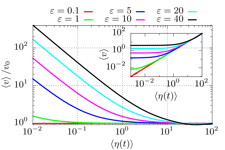
Figure 1: The rescaled average velocity $\langle v\rangle/v_{0}$, where $v_{0}$ corresponds to the mean velocity of free particle, versus the average $\langle\eta(t)\rangle$ of active fluctuations presented for different barrier height $\varepsilon$ of the periodic potential $U(x)$. In the inset the non-rescaled average velocity $\langle v\rangle$ is depicted as a function of $\langle\eta(t)\rangle$. Parameters read: the spiking rate $\lambda=30$, variance and skewness of the amplitude distribution $\rho(z)$ is $\sigma^{2}=3.1$ and $\chi=0.99$, respectively. Temperature is set to $D_{T}=0.01$.

The main quantity of interest for the study of transport properties is the directed velocity defined as $\langle v\rangle=\lim_{t\to\infty}\langle x(t)\rangle/t$, where $\langle\cdot\rangle$ indicates the ensemble average. If $\eta(t)=0$ in Eq. (2) then $\langle v\rangle=0$. In the presence of active fluctuations with $\langle\eta(t)\rangle=v_{0}$ the free Brownian particle is transported with the average velocity $\langle v\rangle=v_{0}$. If under the identical experimental conditions the periodic potential $U(x)$ is turned on, one expects that the directed velocity will be notably reduced $\langle v\rangle<v_{0}$, in particular for $U(x)$ with large barrier height $\varepsilon$ risken . In Fig. 1 we present a paradoxical effect that contradicts common intuition in which the periodic structure not only does not hinder the directed velocity of the particle, but on the contrary, it is involved in inducing the giant transport which can be several orders of magnitude greater than the velocity of the free particle, i.e., $\langle v\rangle/v_{0}\gg 1$.

We note that for the fixed mean $\langle\eta(t)\rangle$ of active fluctuations the rescaled velocity $\langle v\rangle/v_{0}$ grows when the potential barrier $\varepsilon$ is increased, see Fig. 2. E.g. for $\langle\eta(t)\rangle=0.1$ and $\varepsilon=40$ the particle velocity is two orders of magnitude greater than for the free transport $\langle v\rangle\approx 400v_{0}$. Moreover, the rescaled velocity tends to infinity $\langle v\rangle/v_{0}\to\infty$ when nonequilibrium noise diminishes to zero $\langle\eta(t)\rangle\to 0$. In this sense, the presented phenomenon is an analogue of the celebrated giant diffusion effect reimann2001 ; lindner2016 ; spiechowicz2020pre ; spiechowicz2021pre2 ; bialas2020 , in which diffusion coefficient $D$ of the particle dwelling in a critically tilted periodic potential is divergent $D\to\infty$ if thermal noise intensity tends to zero $D_{T}\to 0$, but now detected for the velocity degree of freedom instead of the coordinate. The origin of this divergence is explained in the inset of the same panel where another counterintuitive effect is revealed. In contrast to the free particle transport, the non-rescaled average velocity does not tend to zero $\langle v\rangle=v_{0}\to 0$ for vanishing mean $\langle\eta(t)\rangle=v_{0}\to 0$ of active fluctuations but when the periodic potential $U(x)$ is switched on it rather goes to the constant plateau $\langle v\rangle\to v_{\varepsilon}$ which grows if the potential barrier $\varepsilon$ is increased. Consequently, $\langle v\rangle/v_{0}\to\infty$ when $\langle\eta(t)\rangle\to 0$. This striking observation suggests that the periodic substrate $U(x)$ plays a crucial role in the detected giant transport behavior. In supl we show that this non-trivial effect is not present if the amplitudes $z_{i}$ of active fluctuations $\eta(t)$ are distributed according to the asymmetric exponential statistics commonly emerging in numerous different contexts.

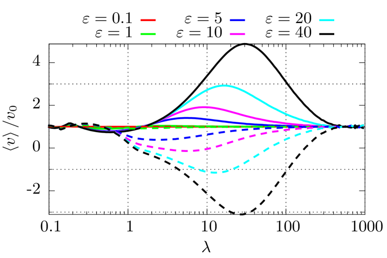
Figure 2: The rescaled average velocity $\langle v\rangle/v_{0}$ versus the spiking rate $\lambda$ of active fluctuations $\eta(t)$ for selected values of the potential barrier height $\varepsilon$ and fixed $\langle\eta(t)\rangle=1$. Solid lines correspond to the asymmetry $\chi=0.99$, whereas dashed ones to $\chi=-0.99$. Other parameters are the variance $\sigma^{2}=3.1$ and temperature $D_{T}=0.01$.

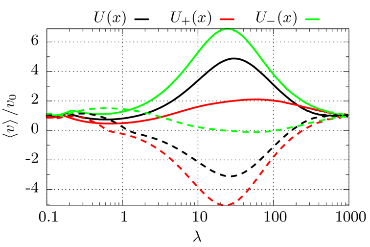
Figure 3: Illustration of the role of potential symmetry on the enhancement of free transport. The potential barrier is $\varepsilon=40$. The average bias $\langle\eta(t)\rangle=1$. Solid lines correspond to the asymmetry $\chi=0.99$, whereas dashed ones to $\chi=-0.99$. Other parameters read: the variance $\sigma^{2}=3.1$ and temperature is fixed to $D_{T}=0.01$.

To explain the mechanism of this phenomenon we first fix the mean of active fluctuations $\langle\eta(t)\rangle=1$ and study how the rescaled velocity $\langle v\rangle/v_{0}$ depends on the spiking rate $\lambda$. This characteristics is depicted in Fig. 2. When the latter quantity either vanishes $\lambda\to 0$ or tends to infinity $\lambda\to\infty$ the average velocity corresponds to the free particle $\langle v\rangle=v_{0}$. Since the bias of nonequilibrium noise is fixed $\langle\eta(t)\rangle=\lambda\zeta=1$ in the former case the average amplitude $\zeta$ of $\delta$-spikes goes to infinity and therefore the potential $U(x)$ becomes negligible. On the other hand, when the frequency $\lambda\to\infty$ one stacks the infinite number of $\delta$-kicks with vanishing mean but the fixed variance $\sigma^{2}=3.1$ and the resultant movement mimics the free particle. The most striking feature of this panel is that for growing potential barrier $\varepsilon$ there is the optimal spiking rate $\lambda_{max}(\varepsilon)$ for which the rescaled velocity is maximal and significantly greater than the free particle transport $\langle v\rangle/v_{0}>1$. We stress that for smaller values of $\langle\eta(t)\rangle$ one observes the giant enhancement $\langle v\rangle/v_{0}\gg 1$, c.f. Fig. 1. The effect of $\varepsilon$-increase is two-fold. Firstly, it shifts the optimal $\lambda_{max}(\varepsilon)$ towards the larger values and secondly, the magnitude of the velocity enhancement grows at $\lambda=\lambda_{max}(\varepsilon)$.

One can observe there also the impact of the asymmetry $\chi$ of the amplitude distribution $\rho(z)$ supl . At first glance it may seem that the transport direction is completely determined by the sign of mean $\langle\eta(t)\rangle=\lambda\zeta$ of active fluctuations which is controlled by the average value $\langle z_{i}\rangle=\zeta$ of $\delta$-spikes distributed according to the probability density $\rho(z)$. However it is not true in general. In particular, even though the statistical bias reads $\langle\eta(t)\rangle=1$, when $\chi$ is reversed from the positive $\chi=0.99$ to negative one $\chi=-0.99$ the transport direction is also inverted, i.e. $\langle v\rangle<0$. Therefore we conclude that in the studied case the orientation of long tail in $\rho(z)$ is responsible for pointing the direction of particle movement supl . When the asymmetry is negative the transport enhancement over the velocity of free particle $\langle v\rangle/v_{0}>1$ is still observed, however, its magnitude is a little bit smaller than for the situation when $\chi$ is positive.

The next factor which can additionally boost the particle velocity is related to the potential symmetry. This issue is presented in Fig. 3 for three forms of the periodic potential given in Eq. (3): $U(x)$ is symmetric whereas both $U_{+}(x)$ and $U_{-}(x)$ depict the asymmetric ratchet luczka1995 . Their graphs are visualized in supl . The most important conclusion is that the giant increase of free transport depends on the particular realization of periodic substrates and for an appropriate choice it can be even further amplified. E.g. for the ratchet $U_{-}(x)$ the rescaled velocity $\langle v\rangle/v_{0}$ is noticeably larger than for the symmetric potential $U(x)$. By comparing these three substrates we observe that the distance between the maximum $x_{max}$ and minimum $x_{min}>x_{max}$ is greater for the ratchet $U_{-}(x)$ than for the symmetric potential. Conversely, for $U_{+}(x)$ it is smaller than for $U(x)$. It is more likely that active fluctuations $\eta(t)$ will kick out the particle on the longer slope of the potential. Therefore if $\chi=0.99$ and the transport occurs in the positive direction, the rescaled velocity $\langle v\rangle/v_{0}$ for $U(x)$ is greater than for $U_{+}(x)$ and smaller than for $U_{-}(x)$. As we just explained when $\chi=-0.99$ the particle moves in the negative direction and the situation is reversed.

In Fig. 4 we present the exemplary Brownian particle trajectory in the studied parameter regime with $\langle\eta(t)\rangle=1$ and the large potential barrier $\varepsilon=40$. Its careful inspection suggests that the occurring transport process may be decomposed onto two contributions. The first one is associated with the arrival of $\delta$-kick because of which the particle overcomes the potential barrier. In principle in this way it can be carried over its many spatial periods. However, the second one which is clearly missing for the free particle, is related to its relaxation towards the nearest potential minimum as it is e.g. for $t\approx 2.6$ or $t\approx 5.6$. This contribution is at the root of the giant transport effect. When the mean value $\langle\eta(t)\rangle$ of active fluctuations is large then regardless of the potential barrier $\varepsilon$ magnitude the particle velocity attains its free transport value $\langle v\rangle/v_{0}=1$, c.f. Fig 1. It is due to the fact that in such a limit the contribution coming from the relaxation is negligible. However, when $\langle\eta(t)\rangle$ is small, see e.g. $\langle\eta(t)\rangle=0.1$ in Fig. 1, the sliding towards the potential minima plays an essential role and the giant transport occurs when the potential barrier $\varepsilon$ is increased.

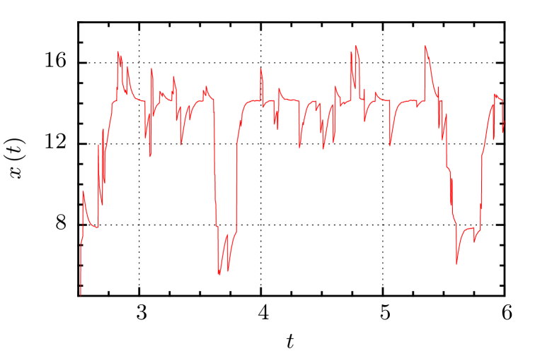
Figure 4: Exemplary Brownian particle trajectory is shown for the potential barrier $\varepsilon=40$. Other parameters read the spiking rate $\lambda=30$, the average bias $\langle\eta(t)\rangle=1$, the variance $\sigma^{2}=3.1$ and asymmetry $\chi=0.99$ of the amplitude distribution $\rho(z)$. Temperature is fixed at $D_{T}=0.01$.

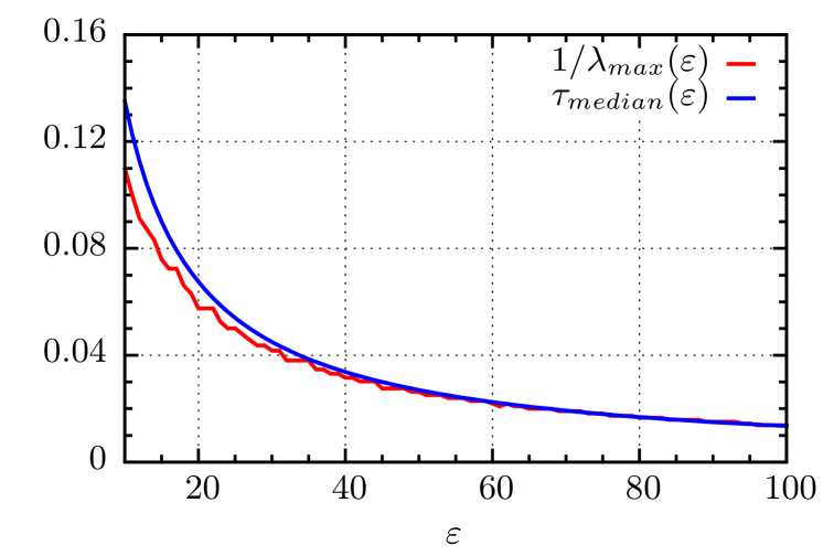
Figure 5: The characteristic time $1/\lambda_{max}(\varepsilon)$ between two successive $\delta$-kicks of active fluctuations $\eta(t)$ and the estimated median time $\tau_{median}(\varepsilon)$ of particle relaxation towards the potential $U(x)$ minimum supl both as a function of the barrier height $\varepsilon$. Other parameters read: the average value of active fluctuations $\langle\eta(t)\rangle=1$, variance $\sigma^{2}=3.1$ and skewness $\chi=0.99$ of the amplitude distribution $\rho(z)$, temperature $D_{T}=0.01$.

To illustrate this fact we ask about the physical interpretation of the optimal spiking rate $\lambda_{max}(\varepsilon)$ for which the rescaled particle velocity $\langle v\rangle/v_{0}$ assumes its maximal value when $\langle\eta(t)\rangle$ is fixed. In Fig. 5 we present inverse of this characteristics $1/\lambda_{max}(\varepsilon)$ and the estimated median time $\tau_{median}(\varepsilon)$ of particle relaxation towards the potential minimum supl both versus the barrier height $\varepsilon$. One can clearly see that the initial discrepancy between these two characteristic time scales quickly dies out as $\varepsilon$ is increased and they become equivalent when the giant transport is detected. Such resonance-like behaviour explains the mechanism of this counterintuitive effect. It means that the enhancement of particle velocity over free transport is maximal when the average time $1/\lambda_{max}(\varepsilon)$ between two successive $\delta$-kicks of active fluctuations matches the interval $\tau_{median}(\varepsilon)$ needed for the particle to exploit the process of relaxation towards the potential $U(x)$ minimum. The resulting motion is synchronized: the particle is $\delta$-kicked and fall on one of the potential $U(x)$ slopes, in the next time interval statistically there are no other $\delta$-spikes and it relaxes to a neighbouring minimum of $U(x)$ and this scenario repeats over and over again. In supl we demonstrate that this mechanism is non-trivial and does not emerge e.g. for the exponential statistics $\rho(z)$ of active fluctuations $\eta(t)$ amplitudes $z_{i}$ which is also asymmetric distribution arising in numerous different contexts.

The proposed strategy for giant boost of free transport allows to understand why sometimes the existence of periodic structures is beneficial for the transport efficiency. Many transport processes in biological cells are driven by diffusion and consequently their effectiveness is low. Therefore cells have developed another mechanism of movement via microtubules that are asymmetric periodic structures which provide platforms for intracellular transport mediated by molecular motors. These platforms can be formed rapidly in response to cellular needs. They have a half-life of 5-10 minutes motor and typically are nucleated and organized by microtubule-organizing centres. The polarized structure of microtubules provide the navigational information necessary to direct cargo to the proper destination in the cell. The biological motor such as a conventional kinesin moves along a microtubule of period 8 nm with a directed velocity 1800 nm/s. Our conclusion is that as Nature teaches us, transport within periodic structures can be many orders of magnitude more efficient than without it. Whether Nature takes advantage of this possibility is another matter, of course.

In summary, we demonstrated a paradoxical effect in which velocity of a free Brownian particle exposed to active fluctuations might be enormously accelerated when it is placed in a periodic potential. Its origin lies in versatile nature of active nonequilibrium fluctuations which allow them to fine-tune to the given substrate and transport the particle across the potential barrier where it is able to effortlessly exploit its steepness. This phenomenon should be contrasted with celebrated giant diffusion effect in which thermal equilibrium fluctuations cooperate with a tilted periodic potential to accelerate diffusion of a particle by many orders of magnitude as compared to free thermal diffusion.

We considered a paradigmatic model of nonequilibrium statistical physics which comprises numerous realizations risken and therefore we expect that our results will inspire a vibrant follow up works. Moreover, the findings may be corroborated experimentally in dissipative optical environment in which the potential barrier can be easily tuned park2020 ; paneru2021 . Our results carry impactful consequences not only for microscopic physical systems, but also biological ones such as molecular motors which are in situ immersed in unavoidable sea of thermal and active fluctuations. Finally, they may open new avenues for designing ultrafast and efficient micro and nanoscale machines.

This work has been supported by the Grant NCN No. 2017/26/D/ST2/00543 (J. S.).

Supplemental Material: Periodic potential can enormously boost
free particle transport induced by active fluctuations

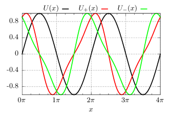
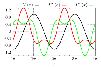
Figure S1: Three forms of the periodic potential $U(x)$, $U_{+}(x)$, $U_{-}(x)$ and corresponding forces, see Eq. (3) in the main text.

I Dimensionless units

Transforming the equation describing the model into its dimensionless form allows to simplify the analysis because it can reduce the number of parameters appearing before such a procedure. Moreover, the resulting representation is independent of a specific experimental setup allowing to choose the best platform for corroborating theoretical predictions. We start with the Langevin equation for an overdamped Brownian particle in a periodic potential $U(x)$ immersed in both active $\eta(t)$ and thermal $\xi(t)$ bath

$$\Gamma\dot{x}=-E\,U^{\prime}(x)+\eta(t)+\sqrt{2\Gamma k_{B}T}\,\xi(t)$$ (S1)

here $\Gamma$ is the friction coefficient, $E$ half of the potential barrier height, $k_{B}$ the Boltzmann constant and $T$ denotes thermostat temperature. The potential is assumed in the periodic form

$$U(x)=U(x+L)$$ (S2)

We rescale the position and time in the following way

$$\hat{x}=2\pi\frac{x}{L},\quad\hat{t}=\frac{t}{\tau_{0}},\quad\tau_{0}=\frac{L}{100v_{D_{0}}}=\frac{L}{100D_{0}/L}=\frac{L^{2}}{100k_{B}T/\Gamma}$$ (S3)

where $v_{D_{0}}$ is the characteristic velocity corresponding to free thermal diffusion $D_{0}=k_{B}T/\Gamma$. The additional multiplier $100$ is introduced in the denominator due to technical reasons outlined below. Under such a choice of the scales Eq. (S1) becomes

$$\dot{\hat{x}}=-\varepsilon\hat{U}^{\prime}(\hat{x})+\hat{\eta}(\hat{t})+\sqrt{2D_{T}}\,\hat{\xi}(\hat{t}).$$ (S4)

where the dimensionless barrier height is $\varepsilon=E/(100k_{B}T)$. The rescaled potential reads

$$\hat{U}(\hat{x})=U\left(\frac{L}{2\pi}\hat{x}\right).$$ (S5)

E.g. if $U(x)=\sin{(2\pi x/L)}$ then $\hat{U}(\hat{x})=\sin{\hat{x}}$ possesses the spatial period $2\pi$. The scaling procedure allows to reduce a number of free parameters by

$$\gamma=1,\quad D_{T}=0.01.$$ (S6)

Dimensionless thermal noise

$$\hat{\xi}(\hat{t})=\frac{L}{2\pi}\frac{1}{100k_{B}T}\,\xi(\tau_{0}\hat{t}).$$ (S7)

exhibits the same statistical properties as the dimensional one, i.e., it has the same vanishing mean and correlation function. The rescaled Poissonian shot noise becomes

$$\hat{\eta}(\hat{t})=\frac{L}{2\pi}\frac{1}{100k_{B}T}\,\eta(\tau_{0}\hat{t}),$$ (S8)

and is characterized by the dimensionless spiking rate

$$\hat{\lambda}=\tau_{0}\lambda.$$ (S9)

Unfortunately, the Fokker-Planck-Kolmogorov-Feller integro-differential equation corresponding to Eq. (S4) cannot be solved analytically in a closed form hanggi1978 . Therefore we resort to precise numerical simulations done by harvesting the GPU supercomputer using the CUDA enviroment spiechowicz2015cpc . The ensemble averaging was performed over Gaussian $\hat{\xi}(\hat{t})$ and Poissonian $\hat{\eta}(\hat{t})$ noise realizations as well as over the initial conditions $\hat{x}(0)$ distributed uniformly over the spatial period $[0,2\pi]$ of the potential $\hat{U}(\hat{x})$.

The error of numerical integration scheme to solve stochastic differential equations driven by Poissonian white shot noise as well as the computation time increases significantly when the frequency $\hat{\lambda}$ of $\delta$-kicks grows kim2007 . To reduce this drawback we introduced the additional multiplier $100$ in the definition of characteristic time scale $\tau_{0}$ which allows to limit the range of spiking rate $\hat{\lambda}$ needed in this study. As in the main text only the dimensionless quantities are used we omit there the hat notation.

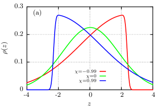
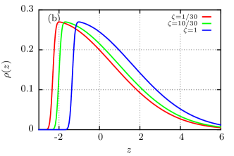
Figure S2: The probability distribution $\rho(z)$ of amplitudes $z_{i}$ of active nonequilibrium fluctuations $\eta(t)$ is presented for fixed mean $\zeta=1/30$ and variance $\sigma^{2}=3.1$ and for different values of skewness $\chi$ in panel (a), and for various mean $\zeta$ with skewness $\chi=0.99$ in panel (b).

II Parametrization of amplitude distribution $\rho(z)$

The skew-normal distribution sp_azz is usually defined in terms of a location $\mu$ representing the shift, a scale $\omega$ proportional to the variance and a parameter $\alpha$ describing the shape. The probability density function then reads

$$\rho(z)=\frac{2}{\sqrt{2\pi\omega^{2}}}e^{-\frac{(z-\mu)^{2}}{2\omega^{2}}}\int_{-\infty}^{\alpha[(z-\mu)/\omega]}ds\,\frac{1}{2\pi}e^{-\frac{s^{2}}{2}}.$$ (S10)

The quantities $\mu$, $\omega$ and $\alpha$ can be represented by more intuitive parameters, namely, the mean $\mu\to\zeta=\langle z_{i}\rangle$, variance $\omega\to\sigma^{2}=(z_{i}-\langle z_{i}\rangle)^{2}$ and skewness $\alpha\to\chi=\langle[(z_{i}-\langle z_{i}\rangle)/\sigma]^{3}\rangle$ of the distribution $\rho(z)$. The average amplitude $\zeta$ allows for direct control of mean bias $\langle\eta(t)\rangle=\lambda\zeta$ of nonequilibrium noise, the variance $\sigma^{2}$ describes the mean square deviation of $\delta$-spikes and skewness $\chi$ measures the asymmetry of skew-normal distribution. Expressions for the location $\mu$, scale $\omega$ and shape $\alpha$ in terms of these parameters are as follows sp_generacja ; sp_generacja2

$$\begin{split}\alpha&=\frac{\delta}{\sqrt{1-\delta^{2}}},\\ \end{split}$$ (S11a)

$$\begin{split}\omega&=\sqrt{\frac{\sigma^{2}}{1-2\delta^{2}/\pi}},\\ \end{split}$$ (S11b)

$$\begin{split}\mu&=\zeta-\delta\sqrt{\frac{2\sigma^{2}}{\pi(1-2\delta^{2}/\pi)}},\\ \end{split}$$ (S11c)

where $\delta$ is defined as

$$\delta=\text{sgn}(\chi)\sqrt{\frac{|\chi|^{2/3}}{(2/\pi)\{[(4-\pi)/2]^{2/3}+|\chi|^{2/3}\}}}.$$ (S12)

In Fig. S2 we present the probability density function $\rho(z)$ for amplitudes of active nonequilibrium noise $\eta(t)$ as a function of its parameters, i.e. mean $\zeta$, variance $\sigma^{2}$ and skewness $\chi$. In panel (a) the impact of skewness $\chi$ for the fixed mean $\zeta=1/30$ is shown whereas in (b) the influence of mean $\zeta$ is illustrated for $\chi=0.99$.

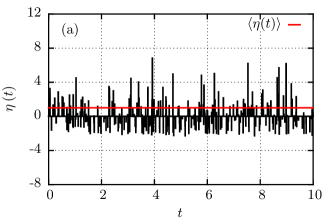
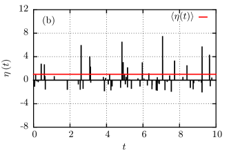
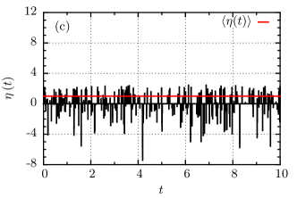
Figure S3: Three exemplary realizations of active nonequilibrium noise $\eta(t)$ for different parameters: (a) $\lambda=30$, $\zeta=1/30$, $\sigma^{2}=3.1$ and $\chi=0.99$; (b) $\lambda=6$, $\zeta=1/6$, $\sigma^{2}=3.1$ and $\chi=0.99$; (c) $\lambda=30$, $\zeta=1/30$, $\sigma^{2}=3.1$ and $\chi=-0.99$. Solid red line corresponds to the average $\langle\eta(t)\rangle=1$.

III Realizations of active fluctuations $\eta(t)$

In Fig. S3 we demonstrate three exemplary realizations of active nonequilibrium noise $\eta(t)$ for different values of its parameters. For all presented cases the statistical bias is fixed to $\langle\eta(t)\rangle=1$. Panel (a) corresponds to the regime of optimal transport $\langle v\rangle/v_{0}$ for the potential barrier height $\varepsilon=40$, see Fig. 2 (a) in the main text, the spiking rate $\lambda=30$, mean amplitude $\zeta=1/30$, variance $\sigma^{2}=3.1$ and skewness $\chi=0.99$. In panel (b) the frequency is five times smaller $\lambda=6$ and therefore $\zeta=1/\lambda=1/6$ to satisfy the condition $\langle\eta(t)\rangle=\lambda\zeta=1$. The reader can indeed infer that the parameter $\lambda$ describes the frequency of $\delta$-spikes whereas an increase of $\zeta$ has two-fold effect: (i) the positive amplitudes $z_{i}>0$ grows and (ii) the negative ones $z_{i}<0$ are reduced. Finally, in panel (c) we present the impact of skewness inversion $\chi\to-\chi$. As it is visualized in this plot such operation corresponds to reflection of the realization about the axis $\eta(t)=0$.

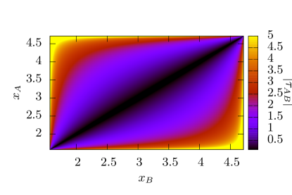
Figure S4: Absolute value of the relaxation time $|\tau_{AB}|$ from the position $x_{A}$ to $x_{B}$ calculated according to Eq. (S14).

IV Estimation of the relaxation time

In absence of all fluctuations the relaxation of the particle towards minimum of the potential $U(x)=\sin(x)$ with the barrier height $\varepsilon$ is determined by the equation

$$\dot{x}=-\varepsilon U^{\prime}(x)=-\varepsilon\cos{x}.$$ (S13)

The time $\tau_{AB}$ the particle needs to move from the point $x_{A}$ to $x_{B}$ reads

$$\tau_{AB}=-\frac{1}{\varepsilon}\int_{x_{A}}^{x_{B}}\frac{dx}{\cos{x}}=-\frac{1}{2\varepsilon}\ln\left|\frac{1+\sin{x}}{1-\sin{x}}\right|\Biggr{|}_{x_{A}}^{x_{B}}.$$ (S14)

After the arrival of $\delta$-spike the particle can land at any random position $x_{A}$ and then during the time interval $\tau_{AB}$ it is relaxing towards the nearest potential minimum. This process ends at the random position $x_{B}$ where another $\delta$-spike of active nonequilibrium noise $\eta(t)$ emerges. As the potential is periodic we restrict ourselves to the interval $x_{A},x_{B}\in\left(\frac{\pi}{2},\frac{3\pi}{2}\right)$. Note that both the minimum and maximum are excluded because the time required to leave the maximum or reach the minimum is infinite and Eq. (S14) does not converge for these values. In Fig. S4 we present the relaxation time $|\tau_{AB}|$ for every pair of the starting and ending point taken from the considered interval $x_{A},x_{B}\in\left(\frac{\pi}{2},\frac{3\pi}{2}\right)$. From this characteristic the mean $\tau_{mean}(\varepsilon)\approx 1.72/\varepsilon$ and median $\tau_{median}(\varepsilon)\approx 1.35/\varepsilon$ of the relaxation time is evaluated.

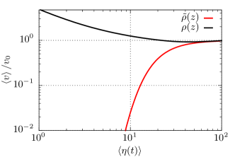
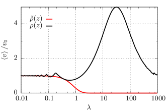
Figure S5: Left panel: The rescaled average velocity $\langle v\rangle/v_{0}$ versus the average $\langle\eta(t)\rangle$ of active fluctuations $\eta(t)$ for two different amplitude statistics, the skew normal $\rho(z)$ and exponential $\tilde{\rho}(z)$ distribution. Right panel: the same characteristics depicted as a function of the spiking rate $\lambda$. Parameters are $\varepsilon=40$, $\sigma^{2}=3.1$, $\chi=0.99$, $D_{T}=0.01$, $\lambda=30$ in the left panel and $\langle\eta(t)\rangle=1$ in the right one.

V Comparison with exponential amplitude distribution $\tilde{\rho}(z)$

In Fig. S5 we present the rescaled average velocity $\langle v\rangle/v_{0}$ for two amplitude statistics of active fluctuations $\eta(t)$, namely the skew normal $\rho(z)$ from the main text and the exponential $\tilde{\rho}(z)$ distribution which is also asymmetric and arises in numerous different contexts and reads

$$\tilde{\rho}(z)=\theta(z)\zeta^{-1}e^{-z/\zeta},$$ (S15)

where $\theta(z)$ is the Heaviside step function. Its statistical moments are given by $\langle z_{i}^{k}\rangle=k!\zeta^{k},\,k=1,2,3...$. In the left panel the rescaled average velocity $\langle v\rangle/v_{0}$ is presented as a function of mean value $\langle\eta(t)\rangle$. The parameter regime is the same as in Fig. 1 in the main text. In contrast to the skew-normal statistics $\rho(z)$, for the exponentially distributed active fluctuations $\eta(t)$ there is no transport enhancement and the particle velocity $\langle v\rangle/v_{0}$ tends either to zero when $\langle\eta(t)\rangle\to 0$ or to unity when the mean value of active fluctuations $\langle\eta(t)\rangle\to\infty$. It means that the velocity of the particle in the periodic potential $U(x)$ driven by $\eta(t)$ with $\tilde{\rho}(z)$ is at most equal to the free transport $\langle v\rangle=v_{0}$. This observation is confirmed also in right panel where the same characteristics is depicted but as a function of the spiking rate $\lambda$.

References

- (1) R. Benzi, A. Sutera and A. Vulpiani, J. Phys. A.: Math. Gen. 14, L453 (1981)
- (2) L. Gammaitoni, P. Hänggi, P. Jung and F. Marchesoni, Rev. Mod. Phys. 70, 223 (1998)
- (3) A. Pikovsky and J. Kurths, Phys. Rev. Lett. 78, 775 (1997)
- (4) B. Lindner, J. Garcia-Ojalvo, A. Neiman and L. Schimansky-Geier, Phys. Rep. 392, 321 (2004)
- (5) J. P. Bouchaud, A. Georges, Phys. Rep. 195, 127 (1990)
- (6) R. Metzler, J. H. Jeon, A. G. Cherstvy and E. Barkai, Phys. Chem. Chem. Phys. 16, 24128 (2014)
- (7) J. Spiechowicz, P. Hänggi and J. Łuczka, New J. Phys. 21, 083029 (2019)
- (8) P. Hänggi, F. Marchesoni, Rev. Mod. Phys. 81, 387 (2009)
- (9) C. J. Olson Reichhardt, C. Reichhardt, Annu. Rev. Condens. Matter Phys. 8, 51 (2017)
- (10) J. Spiechowicz, J. Łuczka, P. Hänggi, Sci. Rep. 6, 30948 (2016)
- (11) L. Machura, M. Kostur, P. Talkner, J. Łuczka and P. Hänggi, Phys. Rev. Lett. 98, 040601 (2007)
- (12) J. Nagel, D. Speer, T. Gaber, A. Sterck, R. Eichhorn, P. Reimann, K. Ilin, M. Siegel, D. Koelle and R. Kleiner, Phys. Rev. Lett. 100, 217001 (2008)
- (13) A. Slapik, J. Łuczka, P. Hänggi, J. Spiechowicz, Phys. Rev. Lett. 122, 070602 (2019)
- (14) J. Spiechowicz and J. Łuczka, Sci. Rep. 7, 16451 (2017)
- (15) J. Spiechowicz and J. Łuczka, Chaos 29, 013105 (2019)
- (16) R. Kubo, Rep. Prog. Phys. 29, 255 (1966)
- (17) U. M. B. Marconi, A. Puglisi, L. Rondoni and A. Vulpiani, Phys. Rep. 461, 111 (2008)
- (18) M. E. Cates, Rep. Prog. Phys. 75, 042601 (2012)
- (19) F. S. Gnesotto, F. Mura, J. Gladrow and C. P. Broedersz, Rep. Prog. Phys. 81, 066601 (2018)
- (20) S. Ramaswamy, Annu. Rev. Condens. Matter Phys. 1, 323 (2010)
- (21) P. Romanczuk, M. Bar, W. Ebeling, B. Lindner and L. Schimansky-Geier, Eur. Phys. J. Spec. Top. 202, 1 (2012)
- (22) M. C. Marchetti, J. F. Joanny, S. Ramaswamy, T. B. Liverpool, J. Prost, M. Rao and R. A. Simha, Rev. Mod. Phys. 85, 1143 (2013)
- (23) C. Bechinger, R. Di Leonardo, H. Löwen, C. Reichhardt, G. Volpe and G. Volpe, Rev. Mod. Phys. 88, 045006 (2016)
- (24) C. Maggi, M. Paoluzzi, N. Pellicciotta, A. Lepore, L. Angelani and R. Di Leonardo, Phys. Rev. Lett. 113, 238303 (2014)
- (25) K. Kanazawa, T. G. Sano, T. Sagawa and H. Hayakawa, Phys. Rev. Lett. 114, 090601 (2015)
- (26) C. Maggi, M. Paoluzzi, L. Angelani and R. Di Leonardo, Sci. Rep. 7, 17588 (2017)
- (27) L. Dabelow, S. Bo and R. Eichhorn, Phys. Rev. X 9, 021009 (2019)
- (28) K. Kanazawa, T. G. Sano, A. Cairoli and A. Baule, Nature 579, 364 (2020)
- (29) Y. Ezber, V. Belyy, S. Can and A. Yildiz, Nat. Phys. 16, 312 (2020)
- (30) T. Ariga, K. Tateishi, M. Tomishige and D. Mizuno, Phys. Rev. Lett. 127, 178101 (2021)
- (31) H. Risken, The Fokker-Planck Equation: Methods of Solution and Applications (Berlin-Heidelberg, Springer-Verlag, 1996)
- (32) S. Lifson and J. L. Jackson, J. Chem. Phys. 36, 2410 (1962)
- (33) J. T. Park, G. Paneru, Ch. Kwon, S. Granick and H. K. Pak, Soft Matter 16, 8122 (2020)
- (34) G. Paneru, J. T. Park and H. K. Pak, J. Phys. Chem. Lett. 12, 11078 (2021)
- (35) See the Supplemental material of the manuscript.
- (36) P. Hänggi, Z. Phys. B 30, 85 (1978)
- (37) J. Spiechowicz, P. Hänggi and J. Łuczka, Phys. Rev. E 90, 032104 (2014)
- (38) K. Białas, J. Łuczka, P. Hänggi and J. Spiechowicz, Phys. Rev. E 102, 042121 (2020)
- (39) K. Białas and J. Spiechowicz, Chaos 31, 123107 (2021)
- (40) W. Feller, An introduction to Probability Theory and its Applications (Wiley, New York, 1970)
- (41) A. O’hagan and T. Leonard, Biometrika 63, 201 (1976)
- (42) A. Azzalini, Scand. J. of Stat. 12 171-178 (1985)
- (43) N. Henze, Scand. J. Stat. 13, 271 (1986)
- (44) D. Ghorbanzadeh, P. Durand and L. Jaupi, in Proceedings of the World Congress on Engineering 1, 113 (2017)
- (45) P. Hänggi, Z. Phys. B 36, 271 (1980)
- (46) P. Reimann, C. Van den Broeck, H. Linke, P. Hänggi, J. M. Rubi and A. Perez-Madrid, Phys. Rev. Lett. 87, 010602 (2001)
- (47) B. Lindner and I. M. Sokolov, Phys. Rev. E 93, 042106 (2016)
- (48) J. Spiechowicz and J. Łuczka, Phys. Rev. E 101, 032123 (2020)
- (49) J. Spiechowicz and J. Łuczka, Phys. Rev. E 104, 034104 (2021)
- (50) J. Łuczka, R. Bartussek, P. Hänggi, EPL 31, 431 (1995)
- (51) A. S. Infante, M. S. Stein, Y. Zhai, G. G. Borisy and G. G. Gundersen, Journal of Cell Science 113, 3907 (2000)

References

- (1) P. Hänggi, Z. Phys. B 30, 85 (1978)
- (2) J. Spiechowicz, M. Kostur and Ł. Machura, Comp. Phys. Commun. 191, 140 (2015)
- (3) C. Kim, E. Lee, P. Hänggi and P. Talkner, Phys. Rev. E 76, 011109 (2007)
- (4) A. Azzalini, Scand. J. of Stat. 12 171-178 (1985)
- (5) N. Henze, Scand. J. Stat. 13, 271 (1986)
- (6) D. Ghorbanzadeh, P. Durand and L. Jaupi, in Proceedings of the World Congress on Engineering 1, 113 (2017)