A Variational Approach to the Quantum Separability Problem

Abstract

We present the variational separability verifier (VSV), which is a novel variational quantum algorithm (VQA) that determines the closest separable state (CSS) of an arbitrary quantum state with respect to the Hilbert–Schmidt distance (HSD). We first assess the performance of the VSV by investigating the convergence of the optimization procedure for Greenberger–Horne–Zeilinger (GHZ) states of up to seven qubits, using both statevector and shot-based simulations. We also numerically determine the CSS of maximally-entangled mixed $X$-states ($X$-MEMS), and subsequently use the results of the algorithm to surmise the analytical form of the aforementioned CSS. Our results indicate that current noisy intermediate-scale quantum (NISQ) devices may be useful in addressing the $NP$-hard full separability problem using the VSV, due to the shallow quantum circuit imposed by employing the destructive SWAP test to evaluate the HSD. The VSV may also possibly lead to the characterization of multipartite quantum states, once the algorithm is adapted and improved to obtain the closest $k$-separable state ($k$-CSS) of a multipartite entangled state.

I Introduction

Entanglement is the principal defining feature of quantum mechanics [1], and a quantitative description of the phenomenon started with Bell’s inequalities [2]. Different measures of entanglement quantify distinct resources, although most require the fulfillment of specific conditions to be considered “good” entanglement measures. These conditions can be defined as a set of axioms, such as the nullification of the measure for separable states, invariance under local unitary operations, and monotonicity under local operations and classical communication (LOCC) [3]. To this end, many entanglement measures have been defined, such as distillable entanglement, entanglement cost, and the entanglement of formation [4, 5]. The difficulty in calculating these measures for generic states lies in their non-closed form, given that they generally include the computation of a minimum over a large Hilbert space, which is typically intractable as the dimension of the system scales. On the other hand, the problem of measuring entanglement is more approachable for pure states, given that even for different entanglement classes, that is under stochastic local operations and classical communication (SLOCC) [5], many different measures of entanglement can be computed.

The simplest system that has been completely characterized is a two-qubit one. An interesting property for two qubits is that only two SLOCC classes exist, one which contains the only type of entanglement possible, i.e. bipartite entanglement, and the other consists of fully separable states, i.e. non-entangled states. The relevant literature for three- and four-qubit pure states, as well as the general multipartite case can be found in Refs. [6, 7, 8, 9], [10, 11, 12, 13, 14], and [15, 16, 17, 8, 18] respectively. Only highly specific mixed states are known to have closed forms of multipartite entanglement measures, such as combinations of GHZ and W states [19], GHZ-symmetric states [20], and $X$-MEMS [21], among a few others. It is also known that any arbitrary teleportation protocol [22], using an arbitrary multipartite entanglement channel requires an entanglement monotone termed localizable concurrence [23], as a quantum resource [24].

We can also relax our specificity of requiring an exact quantifier of entanglement, and focus on whether a particular state is certified to be entangled. This is known as the quantum separability problem, and is in fact deemed to be $NP$-hard, even for the bipartite case [25, 26, 27]. Consequently, verifying a state is fully separable requires that the state is separable with respect to all bipartitions, which implies that the full separability problem is at least as hard as the bipartite separability problem. As a result, we look towards VQAs, which incorporate hybrid quantum–classical computation aimed at harnessing the power of NISQ computers [28], to solve challenging computational problems.

To this end, we describe a novel VQA, the VSV, capable of determining the CSS of an arbitrary quantum state (assuming it can be prepared on a quantum device), with respect to the HSD [29]. In addition, the HSD induces an entanglement measure, denoted as the Hilbert–Schmidt entanglement (HSE) [30, 29]. The HSE is still up for debate whether it is an entanglement monotone [31], however, it could in some cases: quantify the amount of entanglement present in specific states; behave as a separability witness; or else provide useful constructions of entanglement witnesses [32].

We will also briefly mention the prospect of extending the VSV to find the $k$-CSS, while for the time being, the algorithm is designed to find the closest fully separable state, i.e. the 1-CSS, which for the sake of brevity we refer to as the CSS. Although we investigate only qubit systems, the VSV can be adapted to find the CSS for qudit systems, however, this requires an encoding of the $d$-level system onto a 2-level system, as well as adjustments to the gates needed to generate ($k$-)separable qudit states.

The paper is organized as follows: Sec. II consists of definitions for the HSD, the induced HSE measure, and the CSS, along with a discussion on why we use the HSD as our metric for the VSV. In Sec. III, we introduce the framework of the VSV, specifically how minimizing the HSD over the set of fully separable states, with respect to a state $\rho$, leads to the CSS of $\rho$ and its HSE. Since the computation of the HSD requires the calculation of state overlaps, we discuss how this is tackled on a quantum device using the destructive SWAP test [33, 34]. We then introduce the variational form of the algorithm and explain the corresponding bilevel optimization [35] approach. Lastly, we discuss some of the computational complexity aspects of the VSV, such as the scaling of the number of parameters with respect to the dimension of the system. In Sec. IV we present the results of the VSV applied to $n$-qubit GHZ states, ranging from two to seven qubits with statevector optimization, and from two to five qubits with shot-based optimization. We also apply the VSV to two- and three-qubit $X$-MEMS. Since the analytical form of the CSS for $n$-qubit $X$-MEMS is not known, we employed a technique similar to the one in Ref. [11] to surmise the analytical form of the CSS in Appendix A. Furthermore, we show that the genuine multipartite entanglement (GME) concurrence [5] and HSE are not related in the case of three-qubit $X$-States [21]. Finally, in Sec. V, we summarize the results of the paper, and acknowledge the inspiration of the VSV: the quantum Gilbert algorithm (QGA) [36, 37, 38, 32], which is further discussed in Appendix B.

II The Hilbert–Schmidt Distance as a Measure of Entanglement

The HSD between two quantum states $D_{\text{HS}}\left(\rho,\sigma\right)$, is defined as

$$D_{\text{HS}}\left(\rho,\sigma\right)\equiv\Tr{\left(\rho-\sigma\right)^{2}},$$ (1)

which is a non-monotonic Riemannian metric [29]. Using this definition, an entanglement measure can be induced by the HSD [30, 29], denoted as the HSE,

$$E_{\text{HS}}\left(\rho\right)\equiv\underset{\sigma\in\mathcal{C}}{\min}~{}D_{\text{HS}}\left(\rho,\sigma\right),$$ (2)

with the CSS defined as

$$\rho_{\text{CSS}}\equiv\underset{\sigma\in\mathcal{C}}{\arg\min}~{}D_{\text{HS}}\left(\rho,\sigma\right).$$ (3)

where $\mathcal{C}$ is the convex set of states for some degree $k$ of separability. To define it concretely, a state $\rho$ is said to be $k$-separable if it can be written as a convex sum of $k$-separable states, that is

$$\rho=\sum_{i}p_{i}\outerproduct{\Psi_{i}^{k}}{\Psi_{i}^{k}},$$ (4)

where a $k$-separable pure state can be written as a tensor product of $k$-local states

$$\ket{\Psi_{i}^{k}}=\bigotimes_{j=1}^{k}\ket{\psi_{j}},$$ (5)

such that $\ket{\psi_{j}}$ are $k$-separable states on subsets of the $n$-qubit parties [37]. More specifically, states are called biseparable for $k=2$, triseparable for $k=3$, up to fully separable for $k=n$. Although the $k$-CSS (3) (and corresponding HSE (2)) can be distinctly defined for all convex sets of $k$-separable states, as stated in Sec. I, we designed the VSV to find the CSS (and corresponding HSE) of entangled states with respect to the set of fully separable states.

It was proven in Ref. [31] that the HSD is not non-increasing under completely-positive trace-preserving (CPTP) maps, posing a principal question of whether the HSE is a good entanglement measure. Nevertheless, the HSD, and the corresponding HSE, are still useful quantities to investigate, since they are utilized in generalized Bell inequalities [39, 40], while also providing insight into the geometry of entangled states [29, 41]. The HSD is also relatively straightforward to evaluate on a quantum device, since it can be decomposed as

$$\Tr{\left(\rho-\sigma\right)^{2}}=\Tr{\rho^{2}}+\Tr{\sigma^{2}}-2\Tr{\rho\sigma},$$ (6)

coupled with using quantum primitives such as the destructive SWAP test to measure the overlap and purities of $\rho$ and $\sigma$.

On the other hand, while it was shown in Ref. [41] that distance measures, such as the Bures measure of entanglement [29], are directly related to the fidelity [42] of a CSS, the fidelity is a harder quantity to evaluate on both a classical and quantum device [30, 43, 33, 44, 34, 45] when compared with the simplicity of the HSD.

It is also interesting to mention that the HSD is being used for tackling the quantum low-rank approximation problem [46], with applications in principal component analysis and preparing arbitrary mixed states on quantum computers [47].

III Framework of the Algorithm

In our procedure, we designate $\rho$ as being the test state, and $\sigma$ as our trial state(s), which are the states that iteratively approach the CSS. As a result, we choose to prepare separable states on a quantum computer in the following way:

$$\sigma(\bm{p},\bm{\theta},\bm{\phi})=\sum_{i=1}^{s}p_{i}\outerproduct{\psi(\bm{\theta}_{i},\bm{\phi}_{i})}{\psi(\bm{\theta}_{i},\bm{\phi}_{i})},$$ (7)

where

$$\bm{p} =\left(\begin{array}[]{c}p_{1}\\ p_{2}\\ \vdots\\ p_{s}\\ \end{array}\right),~{}\sum\limits_{i=1}^{s}p_{i}=1,~{}p_{i}\in[0,1],$$ (12)

$$\bm{\theta} =\left(\begin{array}[]{c}\bm{\theta}_{1}\\ \bm{\theta}_{2}\\ \vdots\\ \bm{\theta}_{s}\\ \end{array}\right)=\left(\begin{array}[]{cccc}\theta_{11}&\theta_{12}&\cdots&\theta_{1n}\\ \theta_{21}&\theta_{22}&\cdots&\theta_{2n}\\ \vdots&\vdots&\ddots&\vdots\\ \theta_{s1}&\theta_{s2}&\cdots&\theta_{sn}\\ \end{array}\right),~{}\theta_{ij}\in[0,2\pi),$$ (21)

$$\bm{\phi} =\left(\begin{array}[]{c}\bm{\phi}_{1}\\ \bm{\phi}_{2}\\ \vdots\\ \bm{\phi}_{s}\\ \end{array}\right)=\left(\begin{array}[]{cccc}\phi_{11}&\phi_{12}&\cdots&\phi_{1n}\\ \phi_{21}&\phi_{22}&\cdots&\phi_{2n}\\ \vdots&\vdots&\ddots&\vdots\\ \phi_{s1}&\phi_{s2}&\cdots&\phi_{sn}\\ \end{array}\right),~{}\phi_{ij}\in[0,2\pi),$$ (30)

totaling $s(2n+1)$ parameters, where $n$ is the number of qubits and $s$ is the number of separable pure states needed to generate the trial state. Due to Carathéodory’s theorem, we require $s\leq d^{2}$ separable pure states [48, 49, 41], where $d=2^{n}$ is the dimension of the Hilbert space. However, in our simulations we found that $s=d$ suffices to find the CSS of all our test states. $\left\{p_{i},\ket{\psi(\bm{\theta}_{i},\bm{\phi}_{i})}\right\}$ represent the ensemble of separable pure states, which can be decomposed as

$$\ket{\psi(\bm{\theta}_{i},\bm{\phi}_{i})}=\bigotimes_{j=1}^{n}\left(\cos\left(\theta_{ij}\right)\ket{0_{j}}+e^{\imath\phi_{ij}}\sin\left(\theta_{ij}\right)\ket{1_{j}}\right).$$ (31)

A separable pure state can thus be generated on a quantum computer by applying a set of one-qubit gates to the all-zero state:

$$\ket{\psi(\bm{\theta}_{i},\bm{\phi}_{i})}=\bigotimes_{j=1}^{n}U(\theta_{ij},\phi_{ij})\ket{0}_{j},$$ (32)

where

$$U(\theta_{ij},\phi_{ij})=\left(\begin{array}[]{cc}\cos\left(\theta_{ij}\right)&-\sin\left(\theta_{ij}\right)\\[4.30554pt] e^{\imath\phi_{ij}}\sin\left(\theta_{ij}\right)&e^{\imath\phi_{ij}}\cos\left(\theta_{ij}\right)\end{array}\right),$$ (33)

which is equivalent to applying an $R_{y}(\theta_{ij})$ gate followed by an $R_{z}(\phi_{ij})$ gate.

III.1 Measuring the Hilbert–Schmidt Distance

Preparing a mixed state on a quantum computer, requires, in general, twice as many qubits when compared to the size of the state [50]. This, coupled with the issue of preparing an arbitrary separable state, leads us to find an alternative method for computing the overlap of the trial states with the test state. Our solution is to individually supply separable (non-orthogonal) pure states of our separable mixed state on the quantum computer, evaluate the individual overlaps using the destructive SWAP test, and then classically mix them during the optimization procedure. The benefit of this method is that we do not require the direct preparation of the CSS on the quantum computer, as we are only interested in the computation of the HSD.

Suppose, we can decompose the trial state $\sigma$ as in Eq. (7), then we can evaluate the overlap between $\rho$ and $\sigma$ as

$$\Tr{\rho\sigma} =\Tr{\rho\sum_{i=1}^{s}p_{i}\outerproduct{\psi_{i}}{\psi_{i}}}$$

$$=\sum_{i=1}^{s}p_{i}\Tr{\rho\outerproduct{\psi_{i}}{\psi_{i}}}$$

$$=\sum_{i=1}^{s}p_{i}\expectationvalue{\rho}{\psi_{i}}.$$ (34)

If we want to compute the purity of $\sigma$, then

$$\Tr{\sigma^{2}} =\Tr{\sum_{i=1}^{s}p_{i}\outerproduct{\psi_{i}}{\psi_{i}}\sum_{j=1}^{s}p_{j}\outerproduct{\psi_{j}}{\psi_{j}}}$$

$$=\sum_{i,j=1}^{s}p_{i}p_{j}\Tr{\ket{\psi_{i}}\innerproduct{\psi_{i}}{\psi_{j}}\bra{\psi_{j}}}$$

$$=\sum_{i,j=1}^{s}p_{i}p_{j}|\innerproduct{\psi_{i}}{\psi_{j}}|^{2}$$

$$=\sum_{i=1}^{s}p_{i}^{2}+\sum_{i\neq j}^{s}p_{i}p_{j}|\innerproduct{\psi_{i}}{\psi_{j}}|^{2}$$

$$=\sum_{i=1}^{s}p_{i}^{2}+2\sum_{i<j}^{s}p_{i}p_{j}|\innerproduct{\psi_{i}}{\psi_{j}}|^{2}.$$ (35)

The purity of $\rho$ is trivially obtained assuming we can prepare it directly on a quantum computer; given that it is our test state.

III.2 Measuring Overlaps on a Quantum Computer

Given Eqs (34) and (35), we require subroutines in the VSV capable of measuring the purity and overlap of quantum states. Specifically, one can utilize the destructive SWAP test [33, 34] to calculate these quantities. The concept of this procedure stems from the fact that measuring in the Bell basis determines the amount of correlations present between two systems, and it can be shown that it is equivalent to the non-destructive SWAP test [51]. Fig. 1 shows the quantum circuit for performing the destructive SWAP test.

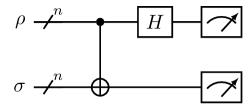
Figure 1: Destructive SWAP test for determining the overlap between two quantum states. The bundled CNOT gate here actually represents CNOT gates between each pair of qubits of $\rho$ and $\sigma$, with the bundled Hadamard gate equating to performing a Hadamard gate on each qubit of $\rho$. This effectively reduces to a Bell basis transformation for each pair of qubits of $\rho$ and $\sigma$.

By placing a CNOT gate followed by a Hadamard gate on the control qubit, each pair of qubits of $\rho$ and $\sigma$ are measured in the Bell basis. Following this, each pair of measurement results are post-processed using the vector $\vec{c}=(1,1,1,-1)$, which corresponds to summing the probabilities of getting 00, 01 and 10, and subtracting the probability of getting 11. This is equivalent to measuring the expectation value of a CZ operator, resulting in obtaining the overlap $\Tr{\rho\sigma}$, as long as the qubits are rearranged as $R_{1}S_{1}R_{2}S_{2}\dots R_{n}S_{n}$, where $R_{i}$ and $S_{i}$ denote the subsystems of $\rho$ and $\sigma$, respectively. This results in a linear scaling in post-processing, given that we do not directly compute $\vec{c}\cdot\vec{p}$, where $\vec{p}$ is the probability vector, but rather binning the paired measurement outcomes into a $+1$ and $-1$ bin, and then averaging the results [34]. The purity of a state can be similarly obtained by supplying two copies of the state as inputs to the test. The one-qubit gates necessary to generate the separable pure states of Eq. (32), coupled with the two-depth circuit needed for the destructive SWAP test, results in a noticeably shallow circuit for the VSV.

III.3 Variational Optimization

Eqs. (34) and (35) give us the means to compute the HSD as in Eq. (6), and by combining these with Eqs. (2) and (3), we can devise a VQA that is able to compute the CSS and the corresponding HSE.

The optimizer in this scenario is tasked with providing angles $\bm{\theta}$ and $\bm{\phi}$ to prepare the separable pure states, and probabilities $\bm{p}$ to classically mix them during post-processing, to generate a separable state $\sigma(\bm{p},\bm{\theta},\bm{\phi})$. One can notice that the quantum computer is only tasked with computing $\Tr{\rho^{2}}$, $\expectationvalue{\rho}{\psi(\bm{\theta}_{i},\bm{\phi}_{i})}$, and $|\innerproduct{\psi(\bm{\theta}_{i},\bm{\phi}_{i})}{\psi(\bm{\theta}_{j},\bm{\phi}_{j})}|^{2}$ $\forall~{}i,j\in[s]$. The probabilities $\bm{p}$ are only incorporated classically when computing the final results for calculating the purity $\Tr{\sigma(\bm{p},\bm{\theta},\bm{\phi})^{2}}$, and the overlap $\Tr{\rho\sigma(\bm{p},\bm{\theta},\bm{\phi})}$. As a result, we split our optimization routine into a bilevel system, which is essentially a nested optimization routine [35].

The structure of the bilevel system is as follows: at the beginning of every iteration, an upper level optimizer selects the parameters $\bm{\theta}$ and $\bm{\phi}$, and proceeds to call the quantum computer to compute the overlaps in Eqs. (34) and (35). The upper level optimizer then launches a lower level optimizer to obtain the parameters $\bm{p}$ to minimize Eq. (6). We thus obtain (near-)optimal parameters of the minimization of the cost function (1),

$$\{\bm{p^{*}},\bm{\theta^{*}},\bm{\phi^{*}}\}\approx\underset{\bm{p},\bm{\theta},\bm{\phi}}{\arg\min}~{}D_{\text{HS}}\left(\rho,\sigma(\bm{p},\bm{\theta},\bm{\phi})\right),$$ (36)

such that the CSS of $\rho$ would then be

$$\rho_{\text{CSS}}\approx\sigma(\bm{p^{*}},\bm{\theta^{*}},\bm{\phi^{*}}),$$ (37)

from which we can calculate the HSE of $\rho$ as

$$E_{\text{HS}}\left(\rho\right)\approx D_{\text{HS}}\left(\rho,\sigma(\bm{p^{*}},\bm{\theta^{*}},\bm{\phi^{*}})\right).$$ (38)

A diagrammatic representation of the VSV algorithm is shown in Fig. 2.

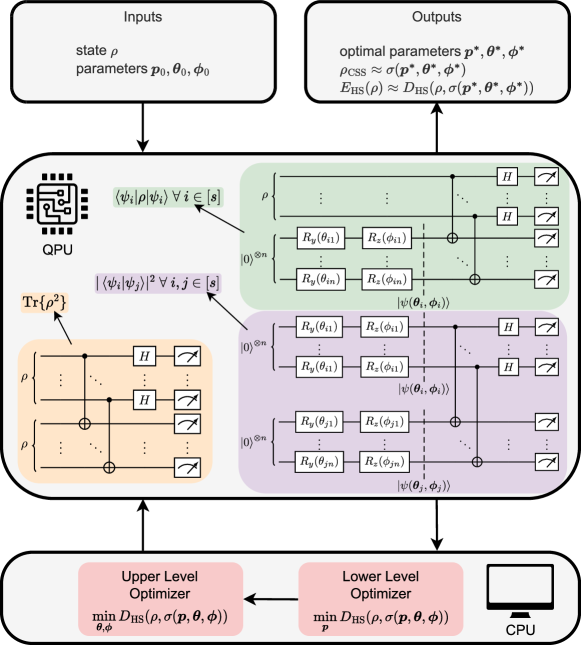
Figure 2: Diagrammatic representation of the VSV. The inputs to the VSV are the test state $\rho$, and initial parameters $\bm{\rho}_{0},\bm{\theta}_{0},\bm{\phi}_{0}$. The VSV then computes the orange (bottom-left QPU) circuit once, to compute $\Tr{\rho^{2}}$, with the green (top-right QPU) and purple (bottom-right QPU) circuits evaluated to compute overlaps $\expectationvalue{\rho}{\psi_{i}}$ and $\innerproduct{\psi_{i}}{\psi_{j}}~{}\forall~{}i,j\in[s]$, which are used in Eqs. (34) and (35), respectively. The red (bottom CPU) section is the classical feedback loop computed by the CPU, consisting of first minimizing the parameters $\bm{p}$, followed by proposing new parameters $\bm{\theta}$ and $\bm{\phi}$ to evaluate on the QPU. After a sufficient number of iterations, the VSV outputs optimal parameters $\bm{\rho^{*}},\bm{\theta^{*}},\bm{\phi^{*}}$, along with the computed CSS and corresponding HSE.

III.4 Complexity Analysis

The scalability of the VSV, similar to other hybrid quantum–classical algorithms, is characterized from both the classical and quantum point of view. The algorithm prepares the test state $\rho$ (which may be unknown, but reproducible) and trial states $\sigma$ on a quantum computer, which provides an exponential memory reduction when compared with purely classical algorithms. We also assume $\rho$ can be efficiently prepared on a quantum device: either via direct input, for example, from another quantum system; or else using quantum state preparation methods [52]. Aside from preparing $\rho$, the algorithm requires $n$ CNOT gates and $n$ Hadamard gates for carrying out the destructive SWAP test, which scales linearly with the number of qubits, and uses a constant circuit depth of two, assuming the quantum computer has a ladder-like connectivity.

In the current implementation of the VSV, the number of parameters scales as $s(2n+1)$ for determining the closest fully separable state of $\rho$, where $s$ is the number of (non-orthogonal) components representing the trial state $\sigma$. Unless $\rho$ is separable, we found that the CSS of $\rho$ being full rank. Thus, we require at least $s\geq d$, although we found that in all of our simulations $s=d$ suffices to find the CSS of an entangled state. This implies that we have an exponential scaling in the number of parameters needed to determine the CSS via this method. This may be alleviated if one finds a way to directly prepare the CSS as a separable mixed state on the quantum device, which will (generally) require doubling the number of qubits [50]. On the other hand, the number of parameters necessary to define the CSS may be reduced such that it scales sub-exponentially with the number of qubits. It should also be noted that finding the $k$-CSS would require more complex ansätze, which are more likely to require a larger set of parameters to represent $k$-separable states.

IV Results

The results involving the VSV are presented in this section for both statevector and shot-based simulations, with all initial points being generated randomly. Statevector simulations refer to instances where we have perfect information about the quantum states (that is access to the vector of the state), which is used to benchmark and test the algorithm. On the other hand, shot-based simulations refer to the cases where we sample the state obtained at the end of each circuit to obtain $N$ bit strings, where $N$ is denoted as the number of shots.

A plot of the HSD convergence using statevector optimization for GHZ states, ranging from two to seven qubits, is shown in Fig. 3 — with an inset similarly showing two to five qubits but using shot-based optimization with 8192 shots. The optimizer used in this instance is the generalized simulated annealing (GSA) algorithm [53, 54] from the SciPy library [55], for upper parameter ($\bm{\theta}$, $\bm{\phi}$) optimization, with the sequential least squares programming (SLSQP) algorithm [56] for the lower parameter ($\bm{p}$) optimizer. The GHZ states are specifically chosen so as to demonstrate the performance of the VSV, and also since the CSS is analytically known, as given in Ref. [32].

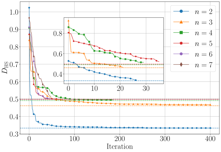
Figure 3: Plot of the convergence of HSD with respect to the number of iterations for the statevector optimization for GHZ states. The solid lines represent the convergence for two to seven qubits (bottom-up). The dashed lines represent the analytical HSE of the corresponding number of qubits, that is $E_{\text{HS}}\left(\ket{\text{\acs{GHZ}}}_{n}\right)$. The inset figure represents the shot-based optimization convergence with 8192 shots for two to five qubits (bottom-up). Note that there are less iterations for the shot-based cases (although same number of function evaluations), since it is harder for the GSA optimizer to find a strictly lower HSE at each function evaluation.

GHZ states are the basis of numerous quantum communication protocols, such as quantum secret sharing [57], and quantum communication complexity reduction [58], beside being the experimental workhorse for more refined tests of quantum non-locality with respect to two-qubit Bell states [59]. GHZ-diagonal states may inherit their non-classical features from the former [60], since they are typically a consequence of local damping channels acting on individual qubits. Thus, investigating the CSS may provide us with a better understanding of the optimal strategies in the presence of noise, as well as insight into the amount of error that is admissible in these protocols, in order to retain a quantum advantage.

The following application of the VSV is on two- and three-qubit $X$-MEMS, which are $X$-states that have the maximal amount of multipartite entanglement for a given linear entropy [21]. These states are specifically chosen since the GME concurrence [5], is known exactly for $X$-states. The GME concurrence is an extension of the bipartite concurrence, which is a measure related to the entanglement of formation [61, 62], and in fact the GME concurrence reduces to the bipartite concurrence for two-qubit states. The intention is to relate the HSE with the GME concurrence, possibly enabling the HSE to behave as an entanglement monotone for $X$-MEMS, albeit it does not satisfy the conditions for one in general [29]. Figs. 5 and 5 show the analytical HSE along with the values determined by the VSV, for two- and three-qubit $X$-MEMS. In the case of the inset figures, the Nakanishi–Fujii–Todo (NFT) optimizer [63] was used as an upper level optimizer, since it offered significant improvement over GSA when evaluating the overlaps using shots rather than statevector calculations.

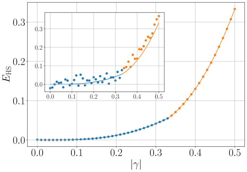
Figure 4: Plot of the results of the statevector optimization applied to two-qubit $X$-MEMS. The solid lines represent the analytical HSE as a function of $|\gamma|$. The left blue segment represents the range between $0\leq|\gamma|\leq\frac{1}{3}$, while the right orange segment represents the range between $\frac{1}{3}\leq|\gamma|\leq\frac{1}{2}$. The inset figure represents the data acquired with shot-based optimization using 8192 shots.

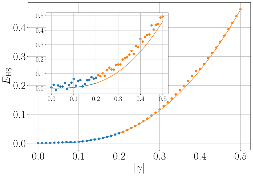
Figure 5: Plot of the results of the statevector optimization applied to three-qubit $X$-MEMS. The solid lines represent the analytical HSE as a function of $|\gamma|$. The left blue segment represents the range between $0\leq|\gamma|\leq\frac{1}{5}$, while the right orange segment represents the range between $\frac{1}{5}\leq|\gamma|\leq\frac{1}{2}$. The inset figure represents the data acquired with shot-based optimization using 8192 shots.

By inspection of the CSS determined by the VSV, we were able to surmise the form of the CSS for $n$-qubit $X$-MEMS, which is

$$\left(\begin{array}[]{cccccccc}\frac{a}{2}&&&&&&&d\\ &\frac{b}{N-1}&&&&&0&\\ &&\ddots&&&\iddots&&\\ &&&\frac{b}{N-1}&0&&&\\ &&&0&\frac{1-a-b}{N-1}&&&\\ &&\iddots&&&\ddots&&\\ &0&&&&&\frac{1-a-b}{N-1}&\\ d^{*}&&&&&&&\frac{a}{2}\\ \end{array}\right),$$ (39)

where $N=2^{n-1}$, $a,b\in[0,1]$, $a+b\leq 1$, and $|d|\in\left[0,\frac{a}{2}\right]$, to ensure a valid density matrix. The parameters $a$, $b$ and $d$ can be directly determined by using the Mathematica code on GitHub [64]. We found that for $n\geq 3$, $a$ is a root of a quartic equation including $\gamma$, with $b$ and $d$ depending on both $a$ and $\gamma$. More details can be found in Appendix A.

Similar to GHZ states and their CSSs (which are also $X$-states), the $X$-state itself is robust against local damping channels [65, 66]. This is due to the fact that decoherence effects that introduce additional non-$X$ elements, to a density matrix, cannot decrease the degree of entanglement [21]. As a consequence, the $X$ part of a density matrix provides a lower bound on the GME present in the state [67]. Furthermore, the possibility of an arbitrary initial pure state decohering into an $X$-state was studied in Ref. [68].

In the case of two-qubit states, the HSE and the concurrence is known to be equal for a restricted set of states [69, 70]. With our VSV, we have numerical evidence supporting the conjecture that the HSE of two distinct, arbitrary, two-qubit states, $\rho$ and $\sigma$, is equal if, and only if, the concurrence of $\rho$ and $\sigma$ is also equal, that is

$$C(\rho)=C(\sigma)\iff E_{\text{HS}}\left(\rho\right)=E_{\text{HS}}\left(\sigma\right),$$ (40)

and similarly, that the HSE of $\rho$ is greater than that of $\sigma$ if, and only if, the concurrence of $\rho$ is also greater than that of $\sigma$, that is

$$C(\rho)>C(\sigma)\iff E_{\text{HS}}\left(\rho\right)>E_{\text{HS}}\left(\sigma\right).$$ (41)

Following this, we tested whether similar statements hold when comparing GME concurrence and HSE for $(n\geq 3)$-qubit $X$-states. All of the simulations we carried out pointed towards the null hypothesis in both cases, meaning that equality does not hold:

$$C_{\text{GME}}(\rho)=C_{\text{GME}}(\sigma)\centernot\iff E_{\text{HS}}\left(\rho\right)=E_{\text{HS}}\left(\sigma\right),$$ (42)

nor does ordered inequality:

$$C_{\text{GME}}(\rho)>C_{\text{GME}}(\sigma)\centernot\iff E_{\text{HS}}\left(\rho\right)>E_{\text{HS}}\left(\sigma\right).$$ (43)

This is not surprising, since the GME concurrence characterizes $n$-qubit entanglement. On the other hand, the HSE seems to describe the departure of a state from a fully separable one, where in the case of three-qubits, may also consist of biseparable states which are not detected by GME concurrence.

V Conclusion

The VSV is a novel VQA that finds the CSS of arbitrary quantum states, with respect to the HSD, and obtain the HSE. The VSV has been applied to $n$-qubit GHZ states, showing the convergence of the optimizer. It has also been applied to investigate $X$-MEMS, producing a relation between the GME concurrence and HSE, as well as helping deduce the analytical form of the CSS for $n$-qubit $X$-MEMS. In this respect, the VSV can be useful for shedding light on possible analytical forms of CSSs for arbitrary states. Further simulations carried out on two-qubit states demonstrated that while equality (or ordering) of the concurrence of two states is present if, and only if, equality (or ordering) of the HSE is also present, this does not hold in general for the GME concurrence and HSE in the case of $X$-states with three or more qubits.

If the calculated HSE of an entangled state is equal to zero, then we trivially acquire $\rho_{\text{CSS}}=\rho$, which immediately implies that our test state $\rho$ is fully separable, and hence, is not entangled. In either case, if one knows the CSS, then an entanglement witness [71, 72, 73] can be defined as $\mathcal{W}\equiv\rho-\rho_{\text{CSS}}$. In general however, one does not exactly acquire the CSS, but rather a close approximation to it, say, $\sigma$. In this case, the optimal entanglement witness would be of the form $\mathcal{W}\equiv\rho-\sigma-\max_{\ket{\psi}\in\mathcal{C}}\expectationvalue{(\rho-\sigma)}{\psi}$ [32].

The strength of the VSV as a potential NISQ algorithm stems from its simplicity. While the algorithm requires in general many calls to the quantum computer for evaluating overlaps, the destructive SWAP test, coupled with the ease of preparing separable states through one-qubit gates, results in a three-depth circuit which is remarkably tractable on a NISQ device. It should be noted that the entire trial state(s) can be directly prepared on the quantum computer by utilizing (up to $n$) ancillary qubits, which are then traced out after performing the relevant unitary gates [50], leading to less overlap computations for the cost of more qubits, as discussed in Sec. III. It is also noteworthy to mention that the evaluation of state overlaps could be improved by looking towards alternative methods, such as in Refs. [74, 75, 76, 77, 78].

Future work would involve enhancing the VSV to find the $k$-CSS of an arbitrary quantum state, which is not straightforward, since even the closest biseparable state for three-qubit states is significantly challenging to implement. The issue lies in properly expressing a biseparable state in a variational form, since the number of pure state bipartitions scales as $2^{n-1}-1$ for an $n$-qubit state. The set of all biseparable states is generated by the convex hull of all pure state bipartitions. This, coupled with the fact that an $n$-qubit state can have rank up to $2^{n}$ makes the extension of the VSV to determine the $k$-CSS extremely non-trivial. The question of finding the $k$-CSS, along with improvements to the performance of the VSV, are left as open problems.

Apart from the VSV, there are alternative approaches that aim to find the CSS of arbitrary states using other methods, such as neural networks [79] and an adaptive polytope approximation [80]. However, work that inspired the variational approach to the problem at hand is the so-called QGA [36, 37, 38, 32]. The implementation of the QGA on a quantum device and related discussion can be found in Appendix B.

The Python code for running the VSV simulations, using the package Qulacs [81], and the Mathematica code for determining the CSS of $X$-MEMS, can be found on GitHub [64].

Appendix A Deriving the CSS for X-MEMS

The general form of $X$-MEMS is given by

$$\tilde{X}=\left(\begin{array}[]{cccccccc}f(\gamma)&&&&&&&\gamma\\ &g(\gamma)&&&&&0&\\ &&\ddots&&&\iddots&&\\ &&&g(\gamma)&0&&&\\ &&&0&0&&&\\ &&\iddots&&&\ddots&&\\ &0&&&&&0&\\ \gamma^{*}&&&&&&&g(\gamma)\\ \end{array}\right),$$ (44)

where

$$f(\gamma) =\begin{cases}\frac{1}{N+1}&0\leq|\gamma|\leq\frac{1}{N+1},\\ |\gamma|&\frac{1}{N+1}\leq|\gamma|\leq\frac{1}{2},\end{cases}$$ (45a)

$$g(\gamma) =\begin{cases}\frac{1}{N+1}&0\leq|\gamma|\leq\frac{1}{N+1},\\ \frac{1-2|\gamma|}{N-1}&\frac{1}{N+1}\leq|\gamma|\leq\frac{1}{2},\end{cases}$$ (45b)

and $N=2^{n-1}$. The GME concurrence was shown to be equal to $2|\gamma|$ for $X$-MEMS [21].

A.1 Two-qubit X-MEMS

The analytical form of the CSS for two-qubit $X$-MEMS was derived using analytical optimization with the Karush–Kuhn–Tucker (KKT) conditions [82], since the numerical results by the VSV hinted towards a CSS of the form

$$\left(\begin{array}[]{cccc}\frac{a}{2}&0&0&d\\ 0&b&0&0\\ 0&0&1-a-b&0\\ d^{*}&0&0&\frac{a}{2}\end{array}\right),$$ (46)

where $a,b\in[0,1]$, $a+b\leq 1$, and $|d|\in\left[0,\frac{a}{2}\right]$, to ensure a valid density matrix. For this state to be separable, then the concurrence must be equal to zero, meaning that

$$|d|^{2}\leq b(1-a-b).$$ (47)

Optimizing this problem results in parameters

$$a =\frac{1}{9}\left(7-\sqrt{1+36|\gamma|^{2}}\right),$$ (48a)

$$b =\frac{1+12|\gamma|^{2}+\sqrt{1+36|\gamma|^{2}}}{6\sqrt{1+36|\gamma|^{2}}},$$ (48b)

$$d =\frac{\gamma}{3}\left(1+\frac{2}{\sqrt{1+36|\gamma|^{2}}}\right),$$ (48c)

with an HSE of

$$E_{\text{HS}}\left(\tilde{X}\right)=\frac{2}{27}\left(1+18|\gamma|^{2}-\sqrt{1+36|\gamma|^{2}}\right),$$ (49)

for $0\leq|\gamma|\leq\frac{1}{3}$, and

$$a =\frac{1}{3}\left(1+4|\gamma|-\sqrt{1-4|\gamma|+8|\gamma|^{2}}\right),$$ (50a)

$$b =\frac{1}{6}\left(3-6|\gamma|+\frac{3-12|\gamma|+16|\gamma|^{2}}{\sqrt{1-4|\gamma|+8|\gamma|^{2}}}\right),$$ (50b)

$$d =\frac{\gamma\left(2-4|\gamma|+\sqrt{1-4|\gamma|+8|\gamma|^{2}}\right)}{3\sqrt{1-4|\gamma|+8|\gamma|^{2}}},$$ (50c)

with an HSE of

$$E_{\text{HS}}\left(\tilde{X}\right) =\frac{2}{3}\left(1-4|\gamma|+6|\gamma|^{2}\right.$$

$$\hskip 24.18501pt+\left.(2|\gamma|-1)\sqrt{1-4|\gamma|+8|\gamma|^{2}}\right),$$ (50d)

for $\frac{1}{3}\leq|\gamma|\leq\frac{1}{2}$.

A.2 Three-qubit X-MEMS

The analytical form of the CSS for three-qubit $X$-MEMS was derived using analytical optimization with the KKT conditions [82], since the numerical results by the VSV hinted towards a CSS of the form

$$\left(\begin{array}[]{cccccccc}\frac{a}{2}&0&0&0&0&0&0&d\\ 0&\frac{b}{3}&0&0&0&0&0&0\\ 0&0&\frac{b}{3}&0&0&0&0&0\\ 0&0&0&\frac{b}{3}&0&0&0&0\\ 0&0&0&0&\frac{1-a-b}{3}&0&0&0\\ 0&0&0&0&0&\frac{1-a-b}{3}&0&0\\ 0&0&0&0&0&0&\frac{1-a-b}{3}&0\\ d^{*}&0&0&0&0&0&0&\frac{a}{2}\end{array}\right),$$ (51)

where similarly, $a,b\in[0,1]$, $a+b\leq 1$, and $|d|\in\left[0,\frac{a}{2}\right]$, to ensure a valid density matrix. Since we require the state to be separable, we first need to certify that the GME concurrence is zero, which results in the same condition as in (47). However, the GME concurrence only assures us that the state does not have tripartite entanglement in this scenario, yet we still need to ensure that the state has no bipartite entanglement. It can be immediately seen from the density matrix (51) that the concurrence between pairs of individual qubits is zero — since the partial trace with respect to each qubit results in a diagonal matrix.

What is left to check is the entanglement between each qubit and the rest, and so, we look to the negativity [83], although the negativity does not capture bound entangled states [71, 84, 85]. However, we conjecture that the state in (51) is not bound entangled, since the numerical HSE, determined by the VSV, coincides with the HSE of (51), as shown in Fig. 5. Due to the uniqueness of the CSS [32], this implies that the fully separable state determined by the VSV, is exactly the same state as (51), meaning that it is fully separable.

The partial transpose of (51) with respect to each qubit is equivalent, and the negativity is non-zero if the partial transpose has negative eigenvalues. Now, the partial transpose of (51) only has one eigenvalue which can be negative, for some parameters $a$, $b$ and $d$, which is

$$\frac{1}{6}\left(1-a-\sqrt{(1-a-2b)^{2}+36|d|^{2}}\right),$$ (52)

meaning we need to ascertain that the above condition is non-negative, for (51) to be separable. This condition can instead be rewritten and shown that it is equivalent to

$$|d|^{2}\leq\frac{b(1-a-b)}{9},$$ (53)

which interestingly encompasses condition (47) as well, resulting in an analytical optimization problem using the KKT conditions with only constraint (53) to insure separability. For the sake of brevity, we shall not provide the parameters $a$, $b$ and $d$, as well as the HSE here, since they are in terms of a root of a quartic equation and so the explicit equations would be too cumbersome to present. Nevertheless, they can be reproduced using the Mathematica code available on GitHub [64].

A.3 n-qubit X-MEMS

While we have not explicitly derived the CSS of $n$-qubit $X$-MEMS in general, we conjecture that it is of the form

$$\left(\begin{array}[]{cccccccc}\frac{a}{2}&&&&&&&d\\ &\frac{b}{N-1}&&&&&0&\\ &&\ddots&&&\iddots&&\\ &&&\frac{b}{N-1}&0&&&\\ &&&0&\frac{1-a-b}{N-1}&&&\\ &&\iddots&&&\ddots&&\\ &0&&&&&\frac{1-a-b}{N-1}&\\ d^{*}&&&&&&&\frac{a}{2}\\ \end{array}\right),$$ (54)

where $N=2^{n-1}$, $a,b\in[0,1]$, $a+b\leq 1$, and $|d|\in\left[0,\frac{a}{2}\right]$, to ensure a valid density matrix. This form is also invariant under the symmetries imposed by $X$-MEMS, which is a necessary condition for the CSS as shown in Ref. [32]. The symmetries of the CSS consist of any qubit permutations from the set $\{2,\dots,n\}$, and the condition that the all-zero element must be equal to the all-one element. The parameter $a$ in the CSS seems to in general be a root of a quartic equation, with the parameters $b$ and $d$ depending on both $a$ and $\gamma$. The condition for zero negativity also encompasses the cases for $(k\geq 3)$-separability, which is equivalent to

$$|d|^{2}\leq\frac{b(1-a-b)}{(N-1)^{2}},$$ (55)

presumably related to the hierarchy of mixed state entanglement [5].

Fig. 6 shows the analytical HSE of two- to nine-qubit $X$-MEMS as a function of $|\gamma|$. Each function for the HSE is piece-wise continuous, with the domains divided at the point $|\gamma|=\frac{1}{N+1}$, as is similarly given by the definition of the $X$-MEMS in Eqs. (45). The CSSs possess an HSE of zero at $|\gamma|=0$ and an HSE of

$$E_{\text{HS}}\left(\ket{\text{\acs{GHZ}}}_{n}\right)=\frac{2^{n}-2}{2^{n+1}+2^{3-n}-4},$$ (56)

at $|\gamma|=\frac{1}{2}$, since the $n$-qubit $X$-MEMS correspond to the $n$-qubit GHZ states at that point [32]. It is also interesting to note the limit of the functions in Fig. 6, corresponding to the infinite-qubit $X$-MEMS, which is equal to

$$\lim\limits_{n\rightarrow\infty}E_{\text{HS}}\left(\tilde{X}_{n}\right)=2|\gamma|^{2},$$ (57)

meaning that the HSE for $X$-MEMS is bounded above.

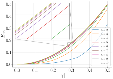
Figure 6: Analytical HSE of two- to nine-qubit $X$-MEMS as a function of $|\gamma|$ (bottom-up). The infinite-qubit (top-most line) case represents the analytical upper bound of $2|\gamma|^{2}$ for the HSE of $X$-MEMS.

Appendix B Comparison with the Quantum Gilbert Algorithm

The QGA is the quantum analogue of Gilbert’s algorithm [86], which is utilized to determine the distance between a given point and a convex set, according to the Hilbert-Schmidt norm. The QGA has insofar only been implemented on classical computers to test for membership of states in different SLOCC classes [36, 37, 38, 32].

It is only natural to attempt to extend the QGA to operate on a quantum computer, owing to many reasons. The first of which is the storage of quantum mixed state data, which is known to increase exponentially as $4^{n}$, with respect to the number of qubits $n$. The second is the input of arbitrary mixed states into a quantum computer, created via open quantum systems as an example, where these reasons also apply to the VQA counterpart. The issue in simply extending the QGA to be utilized on a quantum computer, in order to improve the performance over its classical counterpart, is due to the nature of the algorithm itself, requiring possibly, an infinite number of state mixtures to the trial state. The QGA relies on computing overlaps of different trial states, similar to the VSV, however, the main difference is that the VSV keeps a constant number of states in memory. On the other hand, the QGA, at each successful iteration of the algorithm adds one state to memory, increasing the number of future overlap calculations. This means that more calls to the quantum computer are required for subsequent iterations of the algorithm. In general if we suppose we require one million trial states for a three-qubit state to acquire a reasonable CSS, which is exactly the amount of states taken by the QGA, as given in Ref. [32], and we assume that the number of successes, $c_{s}$, is proportional to the number of trial states, $c_{t}$, by $c_{s}\propto c_{t}^{0.44127}$, then the number of overlaps is equal to

$$\sum_{i=1}^{10^{6}}\sum_{j=1}^{c_{s}^{(i)}}j=\sum_{i=1}^{10^{6}}\frac{c_{s}^{(i)}\left(c_{s}^{(i)}+1\right)}{2},$$ (58)

where $c_{s}^{(i)}$ is the number of successes at iteration $i$, which starts at $1$ for $i=1$, and increases by $1$ every $\frac{c_{t}}{c_{s}}\approx\frac{c_{t}}{c_{t}^{0.44127}}=c_{t}^{0.55873}$ times, which for one million trial states is approximately every $2251$ trial states. However, in the beginning, almost every trial state will correspond to a success, due to the initial state on average lying farther away from the actual CSS. As the number of successes increases, and the state moves closer to the border of the set of separable states, nearer to the CSS, it will be harder to find a closer separable state. But, even if we take it to be split evenly, then this results to be around $3.3\times 10^{10}$ calls to the quantum computer. On the other hand, the VSV calls the quantum computer $5\times 10^{3}$ times to obtain a CSS comparable to the QGA, which would equate to more than $6\times 10^{6}$ calls for the QGA for each call of the VSV.

In either case, we shall describe the direct implementation of the QGA on a quantum device. Given an initial guess in the form of a pure product state $\sigma_{0}=\outerproduct{\psi_{0}}{\psi_{0}}$, after the $n^{\text{th}}$ success, the new CSS $\rho_{n}$ to the test state $\rho$ is given iteratively as

$$\rho_{n}=p_{n}\rho_{n-1}+(1-p_{n})\sigma_{n},$$ (59)

which equates to

$$\rho_{n}=\sum_{i=0}^{n}\left(\prod_{j=i+1}^{n}p_{j}\right)\left(1-p_{i}\right)\sigma_{i},$$ (60)

where $\sigma_{i}=\outerproduct{\psi_{i}}{\psi_{i}}$ is a pure product state and $p_{i}\in(0,1)$, such that

$$\sum_{i=0}^{n}\left(\prod_{j=i+1}^{n}p_{j}\right)\left(1-p_{i}\right)=1.$$ (61)

Note that this definition entails that $\rho_{0}\equiv\sigma_{0}$. The implementation of a QGA can be thus be described as follows [32]:

1. Input data: the state to be tested $\rho$ and any pure product state $\sigma_{0}$.

2. Output data: the closest state found after $n$ successes $\rho_{n}$, and lists of values of $D_{\text{HS}}\left(\rho,\rho_{i}\right)=\Tr{(\rho-\rho_{i})^{2}}$, $p_{i}$ and $\sigma_{i}$.

1. Calculate the value of $D_{\text{HS}}\left(\rho,\sigma_{0}\right)\equiv D_{\text{HS}}\left(\rho,\rho_{0}\right)$ and add it to the list.

2. Increase the counter of trials $c_{t}$ by 1. Draw a random pure product state $\sigma_{1}$, hereafter called the first trial state.

3. Run a preselection for the trial state by checking a value of a linear functional. If it fails, go back to step 1.

4. In the case of successful preselection, find the minimum of $\Tr{(\rho-\rho_{n})^{2}}$ with respect to $p_{n}$, which in the case of the first trial state is $\Tr{(\rho-p_{1}\rho_{0}-(1-p_{1})\sigma_{1})^{2}}$ with respect to $p_{1}$.

5. If the minimum occurs for $p_{1}\in[0,1]$, then $\rho_{1}=p_{1}\rho_{0}+(1-p_{1})\sigma_{1}$ is saved to the list as the new CSS, along with the value of $D_{\text{HS}}\left(\rho,\rho_{1}\right)$, $p_{1}$ and $\sigma_{1}$, increase the success $c_{s}$ counter value by 1.

6. Go to step 1., now drawing a new random pure product state $\sigma_{2}$, such that after a successful preselection, one determines a new $p_{2}$, and consequently $\rho_{2}$, and then saves $D_{\text{HS}}\left(\rho,\rho_{2}\right)$, $p_{2}$ and $\sigma_{2}$. Continue in this fashion until a specified HALT criterion is met.

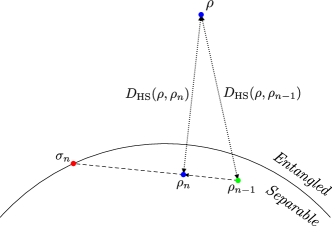
Figure 7: Visualization of the $n^{\text{th}}$ iteration of the QGA. A random pure product state $\sigma_{n}$ is generated that satisfies the preselection criterion. The next step is to find $\rho_{n}=p_{n}\rho_{n-1}+(1-p_{n})\sigma_{n}$, $p_{n}\in(0,1)$, such that $D_{\text{HS}}\left(\rho,\rho_{n}\right)<D_{\text{HS}}\left(\rho,\rho_{n-1}\right)$. Figure adapted from Ref. [32].

Fig. 7 provides a visual representation of the $n^{\text{th}}$ iteration of the algorithm presented above, while the preselection criterion for the $n^{\text{th}}$ trial state is given by

$$\Tr{(\sigma_{n}-\rho_{n-1})(\rho-\rho_{n-1})}>0,$$ (62)

with the geometrical interpretation being that the angle between the vectors $\sigma_{n}-\rho_{n-1}$ and $\rho-\rho_{n-1}$ is not larger than $\frac{\pi}{2}$ [32], ensuring that a state between $\rho_{n-1}$ and $\sigma_{n}$ exists such that it is closer to $\rho$. Eq. (62) can rewritten and computed as

$$\Tr{\rho_{n-1}^{2}}+\Tr{\rho\sigma_{n}}>\Tr{\rho\rho_{n-1}}+\Tr{\rho_{n-1}\sigma_{n}}.$$ (63)

The purity of each new CSS when calculated iteratively (starting at 1 due to the initial trial state $\sigma_{0}$ being a pure state), is given by

$$\Tr{\rho_{n}^{2}} =\Tr{(p_{n}\rho_{n-1}+(1-p_{n})\sigma_{n})^{2}}$$

$$=p_{n}^{2}\Tr{\rho_{n-1}^{2}}+(1-p_{n})^{2}$$

$$\hskip 14.22636pt+2p(1-p_{n})\Tr{\rho_{n-1}\sigma_{n}},$$ (64)

while the overlap is calculated as

$$\Tr{\rho\rho_{n}}=p_{n}\Tr{\rho\rho_{n-1}}+(1-p_{n})\Tr{\rho\sigma_{n}}.$$ (65)

Thus, the cost function for the $n^{\text{th}}$ iteration is defined as follows:

$$D_{\text{HS}}\left(\rho,\rho_{n}\right) =\Tr{(\rho-p_{n}\rho_{n-1}-(1-p_{n})\sigma_{n})^{2}}$$

$$=\Tr{\rho^{2}}+p_{n}^{2}\Tr{\rho_{n-1}^{2}}+(1-p_{n})^{2}$$

$$\hskip 14.22636pt+2p_{n}(1-p_{n})\Tr{\rho_{n-1}\sigma_{n}}$$

$$\hskip 14.22636pt-2p_{n}\Tr{\rho\rho_{n-1}}-2(1-p_{n})\Tr{\rho\sigma_{n}},$$ (66)

which is explicitly written and computed as

$$D_{\text{HS}}\left(\rho,\rho_{n}\right) =D_{\text{HS}}\left(\rho,\sum_{i=0}^{n}\left(\prod_{j=i+1}^{n}p_{j}\right)\left(1-p_{i}\right)\sigma_{i}\right)$$

$$=\Tr{\left(\rho-\sum_{i=0}^{n}\left(\prod_{j=i+1}^{n}p_{j}\right)\left(1-p_{i}\right)\sigma_{i}\right)^{2}}$$

$$=\Tr{\rho^{2}}+\Tr{\left(\sum_{i=0}^{n}\left(\prod_{j=i+1}^{n}p_{j}\right)\left(1-p_{i}\right)\sigma_{i}\right)^{2}}-2\Tr{\rho\sum_{i=0}^{n}\left(\prod_{j=i+1}^{n}p_{j}\right)\left(1-p_{i}\right)\sigma_{i}}$$

$$=\Tr{\rho^{2}}+2\sum_{i<k}^{n}\left(\prod_{j=i+1}^{n}p_{j}\right)\left(\prod_{l=k+1}^{n}p_{l}\right)\left(1-p_{i}\right)\left(1-p_{k}\right)\Tr{\sigma_{i}\sigma_{k}}\ +$$

$$\hskip 14.22636pt\sum_{i=0}^{n}\left(\prod_{j=i+1}^{n}p_{j}^{2}\right)\left(1-p_{i}\right)^{2}-2\sum_{i=0}^{n}\left(\prod_{j=i+1}^{n}p_{j}\right)\left(1-p_{i}\right)\Tr{\rho\sigma_{i}}.$$ (67)

This entails that the overlap between every new trial state $\sigma_{n}$ and every previous trial state $\sigma_{0},\dots,\sigma_{n-1}$, as well as with the test state $\rho$, must be calculated at every iteration. This implies that the parameters of each separable pure trial state must be saved at each success, resulting in an ever-increasing memory and quantum device utilization.

References

- Einstein et al. [1935] A. Einstein, B. Podolsky, and N. Rosen, Phys. Rev. 47, 777 (1935).
- Bell [1964] J. S. Bell, Physics Physique 1, 195 (1964).
- Vedral et al. [1997] V. Vedral, M. B. Plenio, M. A. Rippin, and P. L. Knight, Phys. Rev. Lett. 78, 2275 (1997).
- Plenio and Virmani [2007] M. Plenio and S. Virmani, Proc. Spie. 7, 1 (2007).
- Eltschka and Siewert [2014] C. Eltschka and J. Siewert, J. Phys. A: Math. Theor. 47, 424005 (2014).
- Coffman et al. [2000] V. Coffman, J. Kundu, and W. K. Wootters, Phys. Rev. A 61, 052306 (2000).
- Cunha et al. [2019] M. M. Cunha, A. Fonseca, and E. O. Silva, Universe 5, 209 (2019).
- Gühne and Seevinck [2010] O. Gühne and M. Seevinck, New J. Phys. 12, 053002 (2010).
- Dür et al. [2000] W. Dür, G. Vidal, and J. I. Cirac, Phys. Rev. A 62, 062314 (2000).
- Regula et al. [2014] B. Regula, S. Di Martino, S. Lee, and G. Adesso, Phys. Rev. Lett. 113, 1 (2014).
- Verstraete et al. [2002] F. Verstraete, J. Dehaene, B. De Moor, and H. Verschelde, Phys. Rev. A 65, 052112 (2002).
- Gour and Wallach [2010] G. Gour and N. R. Wallach, J. Math. Phys. 51, 112201 (2010).
- Ghahi and Akhtarshenas [2016] M. G. Ghahi and S. J. Akhtarshenas, Eur. Phys. J. D 70, 1 (2016).
- Osterloh [2016] A. Osterloh, Phys. Rev. A 94, 1 (2016).
- Guo and Zhang [2020] Y. Guo and L. Zhang, Phys. Rev. A 101, 032301 (2020).
- Eisert and Briegel [2001] J. Eisert and H. J. Briegel, Phys. Rev. A 64, 022306 (2001).
- Love et al. [2006] P. J. Love, A. M. v. d. Brink, A. Y. Smirnov, M. H. S. Amin, M. Grajcar, E. Il’ichev, A. Izmalkov, and A. M. Zagoskin, A characterization of global entanglement (2006).
- Walter et al. [2016] M. Walter, D. Gross, and J. Eisert, Multipartite Entanglement (2016).
- Eltschka et al. [2008] C. Eltschka, A. Osterloh, J. Siewert, and A. Uhlmann, New J. Phys. 10, 043014 (2008).
- Eltschka and Siewert [2012] C. Eltschka and J. Siewert, Phys. Rev. Lett. 108, 020502 (2012).
- Agarwal and Hashemi Rafsanjani [2013] S. Agarwal and S. M. Hashemi Rafsanjani, Int. J. Quantum Inf. 11, 1350043 (2013).
- Bennett et al. [1993] C. H. Bennett, G. Brassard, C. Crépeau, R. Jozsa, A. Peres, and W. K. Wootters, Phys. Rev. Lett. 70, 1895 (1993).
- Popp et al. [2005] M. Popp, F. Verstraete, M. A. Martín-Delgado, and J. I. Cirac, Phys. Rev. A 71, 042306 (2005).
- Consiglio et al. [2021] M. Consiglio, L. Z. Mangion, and T. J. G. Apollaro, Int. J. Quantum Inf. 19, 10.1142/s0219749921500246 (2021).
- Gurvits [2004] L. Gurvits, J. Comput. Syst. Sci. 69, 448 (2004), special Issue on STOC 2003.
- Ioannou [2007] L. Ioannou, Proc. Spie. 7, 336 (2007), arXiv:0603199 [quant-ph] .
- Gharibian [2010] S. Gharibian, Proc. Spie. 10, 343 (2010), arXiv:0810.4507 .
- Preskill [2018] J. Preskill, Quantum 2, 79 (2018).
- Bengtsson and Zyczkowski [2006] I. Bengtsson and K. Zyczkowski, Geometry of Quantum States (Cambridge University Press, 2006).
- Witte and Trucks [1999] C. Witte and M. Trucks, Phys. Lett. A 257, 14 (1999).
- Ozawa [2000] M. Ozawa, Phys. Lett. A 268, 158 (2000).
- Pandya et al. [2020] P. Pandya, O. Sakarya, and M. Wieśniak, Phys. Rev. A 102, 012409 (2020).
- Garcia-Escartin and Chamorro-Posada [2013] J. C. Garcia-Escartin and P. Chamorro-Posada, Phys. Rev. A 87, 052330 (2013).
- Cincio et al. [2018] L. Cincio, Y. Subaşı, A. T. Sornborger, and P. J. Coles, New J. Phys. 20, 113022 (2018).
- Dempe [2002] S. Dempe, Foundations of bilevel programming, Nonconvex optimization and its applications, Vol. 61 (Kluwer Academic Publishers, Dordrecht, 2002).
- Brierley et al. [2016] S. Brierley, M. Navascues, and T. Vertesi, Convex separation from convex optimization for large-scale problems (2016).
- Shang and Gühne [2018] J. Shang and O. Gühne, Phys. Rev. Lett. 120, 050506 (2018).
- Wieśniak et al. [2020] M. Wieśniak, P. Pandya, O. Sakarya, and B. Woloncewicz, Quantum Reports 2, 49 (2020).
- Bertlmann et al. [2002] R. A. Bertlmann, H. Narnhofer, and W. Thirring, Phys. Rev. A 66, 032319 (2002).
- Silva and Franco [2022] S. L. L. Silva and D. H. T. Franco, Quantum Studies: Mathematics and Foundations 9, 219 (2022).
- Streltsov et al. [2010] A. Streltsov, H. Kampermann, and D. Bruß, New J. Phys. 12, 123004 (2010).
- Uhlmann [1976] A. Uhlmann, Rep. Math. Phys. 9, 273 (1976).
- Brun [2004] T. A. Brun, Measuring polynomial functions of states (2004).
- Bartkiewicz et al. [2013] K. Bartkiewicz, K. Lemr, and A. Miranowicz, Phys. Rev. A 88, 052104 (2013).
- Cerezo et al. [2020] M. Cerezo, A. Poremba, L. Cincio, and P. J. Coles, Quantum 4, 248 (2020).
- Ezzell et al. [2022a] N. Ezzell, Z. Holmes, and P. J. Coles, The quantum low-rank approximation problem (2022a).
- Ezzell et al. [2022b] N. Ezzell, E. M. Ball, A. U. Siddiqui, M. M. Wilde, A. T. Sornborger, P. J. Coles, and Z. Holmes, Quantum Mixed State Compiling (2022b).
- Horodecki [1997] P. Horodecki, Phys. Lett. A 232, 333 (1997).
- Vedral and Plenio [1998] V. Vedral and M. B. Plenio, Phys. Rev. A 57, 1619 (1998).
- Benenti and Strini [2009] G. Benenti and G. Strini, Phys. Rev. A 79, 052301 (2009).
- Buhrman et al. [2001] H. Buhrman, R. Cleve, J. Watrous, and R. de Wolf, Phys. Rev. Lett. 87, 167902 (2001).
- Araujo et al. [2021] I. F. Araujo, D. K. Park, F. Petruccione, and A. J. da Silva, Sci. Rep. 11, 1 (2021), arXiv:2008.01511 .
- Tsallis and Stariolo [1996] C. Tsallis and D. A. Stariolo, Physica A 233, 395 (1996).
- Xiang et al. [1997] Y. Xiang, D. Sun, W. Fan, and X. Gong, Phys. Lett. A 233, 216 (1997).
- SciPy [2022] SciPy, Dual Annealing, https://docs.scipy.org/doc/scipy/reference/generated/scipy.optimize.dual_annealing.html (2022).
- Kraft [1988] D. Kraft, A Software Package for Sequential Quadratic Programming, Deutsche Forschungs- und Versuchsanstalt für Luft- und Raumfahrt Köln: Forschungsbericht (Wiss. Berichtswesen d. DFVLR, 1988).
- Hillery et al. [1999] M. Hillery, V. Bužek, and A. Berthiaume, Phys. Rev. A 59, 1829 (1999).
- Ho et al. [2022] J. Ho, G. Moreno, S. Brito, F. Graffitti, C. L. Morrison, R. Nery, A. Pickston, M. Proietti, R. Rabelo, A. Fedrizzi, and R. Chaves, npj Quantum Inf. 8, 13 (2022).
- Pan et al. [2000] J.-W. Pan, D. Bouwmeester, M. Daniell, H. Weinfurter, and A. Zeilinger, Nature 403, 515 (2000).
- Chen et al. [2012] X.-y. Chen, L.-z. Jiang, P. Yu, and M. Tian, Entanglement and genuine entanglement of three qubit GHZ diagonal states (2012).
- Hill and Wootters [1997] S. Hill and W. K. Wootters, Phys. Rev. Lett. 78, 5022 (1997).
- Wootters [1998] W. K. Wootters, Phys. Rev. Lett. 80, 2245 (1998).
- Nakanishi et al. [2020] K. M. Nakanishi, K. Fujii, and S. Todo, Phys. Rev. Research 2, 043158 (2020).
- Consiglio [2022] M. Consiglio, https://github.com/mirkoconsiglio/VSV (2022).
- Yu and Eberly [2007] T. Yu and J. Eberly, Proc. Spie. 7, 459 (2007).
- Hashemi Rafsanjani et al. [2012] S. M. Hashemi Rafsanjani, M. Huber, C. J. Broadbent, and J. H. Eberly, Phys. Rev. A 86, 062303 (2012).
- Ma et al. [2011] Z.-H. Ma, Z.-H. Chen, J.-L. Chen, C. Spengler, A. Gabriel, and M. Huber, Phys. Rev. A 83, 062325 (2011).
- Quesada et al. [2012] N. Quesada, A. Al-Qasimi, and D. F. James, J. Mod. Optic. 59, 1322 (2012), https://doi.org/10.1080/09500340.2012.713130 .
- Mundarain and Stephany [2007] D. Mundarain and J. Stephany, Concurrence and negativity as distances (2007).
- Ganardi et al. [2022] R. Ganardi, M. Miller, T. Paterek, and M. Żukowski, Quantum 6, 654 (2022).
- Horodecki et al. [1996] M. Horodecki, P. Horodecki, and R. Horodecki, Phys. Lett. A 223, 1 (1996).
- Doherty et al. [2004] A. C. Doherty, P. A. Parrilo, and F. M. Spedalieri, Phys. Rev. A 69, 022308 (2004).
- Gühne and Tóth [2009] O. Gühne and G. Tóth, Phys. Rep. 474, 1 (2009).
- Flammia and Liu [2011] S. T. Flammia and Y.-K. Liu, Phys. Rev. Lett. 106, 230501 (2011).
- Elben et al. [2019] A. Elben, B. Vermersch, C. F. Roos, and P. Zoller, Phys. Rev. A 99, 052323 (2019).
- Elben et al. [2020] A. Elben, B. Vermersch, R. van Bijnen, C. Kokail, T. Brydges, C. Maier, M. K. Joshi, R. Blatt, C. F. Roos, and P. Zoller, Phys. Rev. Lett. 124, 010504 (2020).
- Fanizza et al. [2020] M. Fanizza, M. Rosati, M. Skotiniotis, J. Calsamiglia, and V. Giovannetti, Phys. Rev. Lett. 124, 060503 (2020).
- Liu and Yin [2022] W. Liu and H.-W. Yin, Physica A 606, 128117 (2022).
- Girardin et al. [2022] A. Girardin, N. Brunner, and T. Kriváchy, Phys. Rev. Research 4, 023238 (2022).
- Ohst et al. [2022] T.-A. Ohst, X.-D. Yu, O. Gühne, and H. C. Nguyen, Certifying Quantum Separability with Adaptive Polytopes (2022).
- Suzuki et al. [2021] Y. Suzuki, Y. Kawase, Y. Masumura, Y. Hiraga, M. Nakadai, J. Chen, K. M. Nakanishi, K. Mitarai, R. Imai, S. Tamiya, T. Yamamoto, T. Yan, T. Kawakubo, Y. O. Nakagawa, Y. Ibe, Y. Zhang, H. Yamashita, H. Yoshimura, A. Hayashi, and K. Fujii, Quantum 5, 559 (2021).
- Tabak and Kuo [1971] D. Tabak and B. C. Kuo (1971).
- Życzkowski et al. [1998] K. Życzkowski, P. Horodecki, A. Sanpera, and M. Lewenstein, Phys. Rev. A 58, 883 (1998).
- Peres [1996] A. Peres, Phys. Rev. Lett. 77, 1413 (1996).
- Horodecki et al. [1998] M. Horodecki, P. Horodecki, and R. Horodecki, Phys. Rev. Lett. 80, 5239 (1998).
- Gilbert [1966] E. G. Gilbert, Siam J. Control 4, 61 (1966).