Online Evasive Strategy for Aerial Survey using Sierpinski curve
Abstract
This paper deals with the aerial survey of a closed region using the Space-Filling curve, particularly Sierpinski curve. The specified region is triangulated, and the Sierpinski curve is used to explore each smaller triangular region. The entire region may have one or more obstacles. An algorithm is presented which suggests evasive manoeuvre (detour) if an obstacle is detected. The algorithm is online; that is, it does not require prior knowledge of the location of obstacles and can be applied while the robotic system is traversing the designated path. The fractal nature of the Sierpinski curve and simple geometric observations were used to formulate and validate the algorithm. The non-uniform coverage and multiple obstacle problems are also dealt with towards the end.
keywords:
Autonomous Vehicles, Coverage Path Planning, Online Obstacle evasion, Robotic Exploration, Space-Filling curve, Trajectory and Path Planning1 Introduction
Space-Filling curves are a special type of curves that pass through every point of closed interval onto which they are mapped. Space-Filling curves are made out of smaller similar curves, which is referred to as the fractal nature of space filling curves (Sagan (1994), Bader (2012)). Due to these interesting properties, space-filling curves are widely used in applications where the agent needs to explore/survey a region and gather data. Other applications of Space-Filling curves can be found in computer graphics (Dafner et al. (2000), Memon et al. (2000)), Computer Aided-Design (Bader (2012)), parallel computing (Zumbusch (2000)) and many more.
With advent of Unmanned Aerial Vehicles (UAVs), the robotics exploration/survey task has been simplified. Survey using UAVs is superior due to the following advantages :
-
1.
The search agent no longer need to worry about the region’s topography.
-
2.
The surface of the region being explored remains undisturbed.
-
3.
Cheaper and less bulky UAVs can be deployed in huge numbers, reducing cost and increasing efficiency in terms of both energy and time.
A survey of a region using aerial vehicles is theoretically better but requires robust algorithms/strategies for implementation in the real world. This paper deals with one such strategy for aerial survey using the Sierpinski curve.
The robotics exploration problem is a sub-problem of the Coverage Path Planning problem (CPPP). In CPPP, a robotic agent needs to traverse through a certain region while doing tasks like mowing, painting, or cleaning, to name a few. There are many solutions available for CPPP which can be used for robotic exploration problem and hence for aerial survey: Boustrophedon decomposition, Grid-based methods, Graph-based methods, and many more (Galceran and Carreras (2013)).
Space-Filling curves provide a novel solution to robotic exploration problem because of their useful properties. An exhaustive search can be carried out since it passes through every point of the region. The fractal nature allows us to design algorithms/strategies easily since a space-filling curve is a combination of other similar space-filling curves. Space-Filling curves can span both 2D and 3D space, and algorithms built for a 2D region can be easily extended to 3D space.
Spires and Goldsmith (1998) suggest the use of a swarm of robots for exploration, each robot following a space-filling curve. This approach is efficient in terms of energy, robust to failures, and assures coverage in finite time, But the presence of obstacles is not considered. Tiwari et al. (2007) and Ban et al. (2013) propose a solution to the exploration problem using a space-filling curve. However, apriori location of obstacles is required making them unsuitable for online implementation. Nair et al. (2017), Joshi et al. (2019) give out online algorithms for robotic exploration using Hilbert’s space-filling curve. However, the obstacles must occupy only single and double neighboring grid locations. But, this approach cannot be used for the Sierpinski curve. So, No online exploration strategy exists for an agent following a Sierpinski curve.
We have formulated a strategy for aerial survey when the search agent uses the Sierpinski curve as a guiding path while avoiding obstacles; when the location of obstacles is unknown. The suggested strategy is online; that is, the whereabouts of the obstacles are unknown when the search is initiated, and the strategy comes into play once it detects the obstacles. The details of strategy implementation in multiple obstacle situations and non-uniform coverage scenarios are established. Finally, the strategy is put together as a pseudo-code for real-life applications.
Section 2 introduces various preliminaries on the Sierpinski curve and other tools required in the following sections. Section 3 formulates the problem and presents the strategy. Various lemmas for validating the result are produced in this section. Section 4 touches upon multiple obstacle scenarios. Section 5 gives out the pseudo-code for implementation of the strategy, and the non-uniform coverage problem is dealt with in brief. Lastly, Section 6 concludes the paper.
2 Preliminaries
2.1 Sierpinski Curve
Sierpinski curve is a mapping from to , where
| (1) |
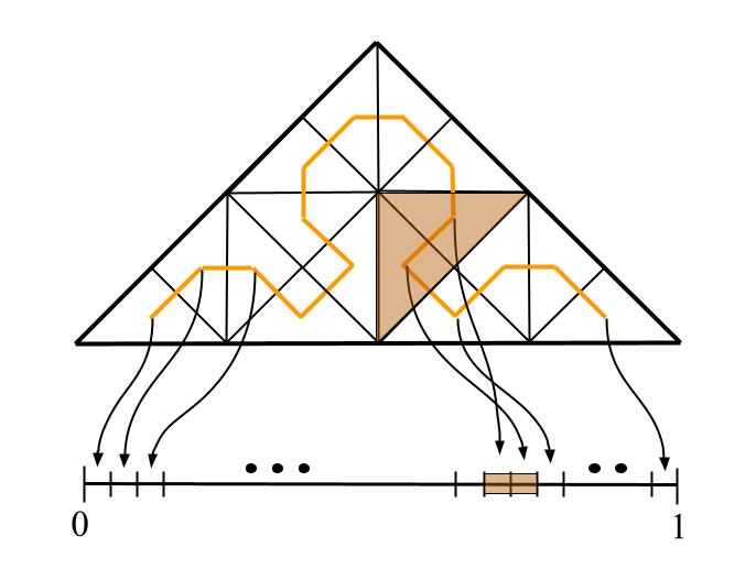
In this paper, we will use approximations of the Sierpinski curve. The approximate Sierpinski curve can be constructed by dividing T into smaller triangles and connecting them in a certain fashion, see figure 1. I is also divided into smaller sub-intervals, which are then mapped to the smaller sub-regions, see figure 2. Here, the refinement of tessellation used for constructing the Sierpinski curve is quantified by iteration number (denoted as ). In figure 1, Sierpinski curve has right triangle divided times, Sierpinski curve has right triangle divided times, and so on. As , approximate Sierpinski curve tends to Sierpinski curve.
A robotic agent with point size sensing radius will require to follow the Sierpinski curve with iteration number going to . However, a search agent with a finite non-zero sensing radius going from one center of triangle to another following the approximate Sierpinski curve can explore T entirely, given it can explore the entire triangular cell it is present in.

2.2 Grammar-based construction of Sierpinski curve
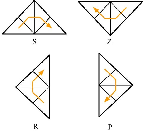
The fractal nature of the Sierpinski curve can be used for its construction. Consider patterns , , , and , as shown in figure 3. Here, is the iteration of Sierpinski curve. Now, using the following production rules, further odd-numbered iterations of the Sierpinski curve can be constructed:
| (2) |
| (3) |
| (4) |
| (5) |
Higher iterations can be constructed in the following way:
Similar patterns and production rules exist for even-numbered iteration Sierpinski curves (Bader (2012)).
There is another way to look at the fractal nature of the Sierpinski curve. It is easy to observe that the iteration 2 Sierpinski curve can be obtained by putting two iteration 1 Sierpinski curves along the shorter side symmetrically and joining the ends. To generalize, iteration Sierpinski curve can be obtained by combining two iteration Sierpinski curves. It is not hard to prove the previous statement. The patterns and the production rules introduced previously can be easily used to prove the statement.
2.3 Extension to Generalised Sierpinski curve
The Sierpinski curve generated in the previous subsection spans an isosceles right triangle (T). However, we are interested in the Sierpinski curve spanning a random triangle, referred to as the Generalised Sierpinski curve (abbreviated as GSc). Patterns and production rules similar to the ones introduced in the last subsection exists for GSc.
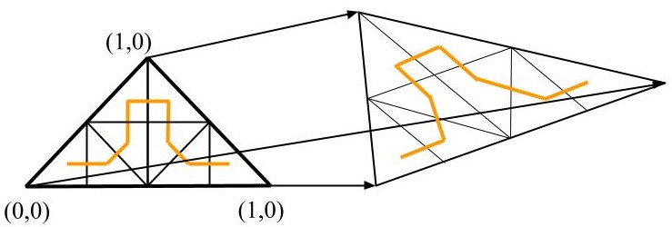
Working with GSc using patterns and production rules can get complicated. Instead we introduce a simple method for generating GSc. Here, the Sierpinski curve for T is generated and converted to GSc spanning a known triangle (denoted as U) using projective transformation (see Kanatani et al. (2016)), as shown in figure 4. Projective transformation is a linear map given by equation 6.
| (6) |
Here, mapped to . , , , , and are constants for given U, and can be calculated by mapping vertices of U, which are already known.
3 Main Result
3.1 Problem Formulation
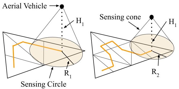
The search agent, which in this case is an aerial vehicle, travels through U using the path marked by GSc. The sensing radius of the search agent and the iteration of GSc are to be decided by the user. The sensing radius and the iteration of GSc are chosen such that the search agent is able to search the entire triangular cell it is present in (See figure 5). The iteration of GSc depends on how rigorously the user wants the search agent to survey a certain part of the region (Further details can be found in Section 5).
In this paper, we assume the obstacles to block single triangular cells in the GSc, and that the search agent detects those obstacles before bumping into them. We further assume that the search agent is equipped with a sensing mechanism to detect obstacles.
While traversing the GSc, the search agent at triangular cell detects obstacle at triangular cell. So, the search agent has to go around the obstacle cell to reach triangular cell and thus successfully evade the obstacle. The search agent may have multiple choices of evasive maneuvers, and the best will be the least lengthy.
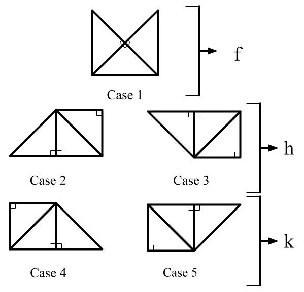
So, the problem boils down to planning evasive maneuvers between the and triangular cells, with the cell blocked by an obstacle. The possible cases of 3 consecutive triangular cell geometries in the Sierpinski curve are listed in figure 6.
Lemma 1
Case 1-5 are the only possible 3 consecutive triangular cell geometries in the Sierpinski curve.
The fractal nature of Sierpinski curve can be used here. It is easy to observe that the case 2-5 are the only cases possible in pattern , , and . Finally, the geometries generated after joining , , and also contains case 1-5 only. Therefore, cases 1-5 are the only possible 3 consecutive triangular geometries in the Sierpinski curve. Since projective transformation is a linear map, the previous statement also holds for GSc, with the perpendicular bisectors in cases 1-5 turning into medians (Line joining a vertex to the mid-point of the opposite side).
Here, case 1 is tagged . Cases 2 and 3 are similar; since they are water images, they are tagged as . Similarly, Cases 4 and 5 are tagged as . Finally, some nomenclature:
-
1.
: Centre of the triangular cell.
-
2.
: Common vertex shared by all 3 triangular cells in each case 1-5.
-
3.
: Vertex shared by and triangular cells only.
-
4.
: Vertex of triangular cell not shared with triangular cell.
Finally, algorithm 1 can be used to tag 3 consecutive triangular cells beginning with cell. {algorithm} Algorithm for tag generation
3.2 Proposed Strategy and Validity of Proposed Strategy
| Sr. No. | Evasive Maneuver | Change of Path | |
|---|---|---|---|
| 1 | ![[Uncaptioned image]](/html/2209.01426/assets/figures/fig8.jpg) |
C | |
| 2 | ![[Uncaptioned image]](/html/2209.01426/assets/figures/2.jpg) |
C | |
| 3 | ![[Uncaptioned image]](/html/2209.01426/assets/figures/3.jpg) |
||
| 4 | ![[Uncaptioned image]](/html/2209.01426/assets/figures/4.jpg) |
C | |
| 5 | ![[Uncaptioned image]](/html/2209.01426/assets/figures/5.jpg) |
Evasive maneuvers are proposed in Table 1. quantifies the length of maneuvers. Case 2 has been used for visualizing maneuvers for tag . Case 4 has been used for visualizing maneuvers for tag . The algorithm for online implementation is presented in Section 5.
Lemma 2
Only the first two and the last two triangular cells in GSc have all three vertices on the boundary of U. Also, only and triangular cells (both from start and end of GSc) share two vertices, both of which lie on the boundary.
The lemma is proved for the Sierpinski curve spanning T. Since the transformation from T to U is linear, the statement would hold for GSc.
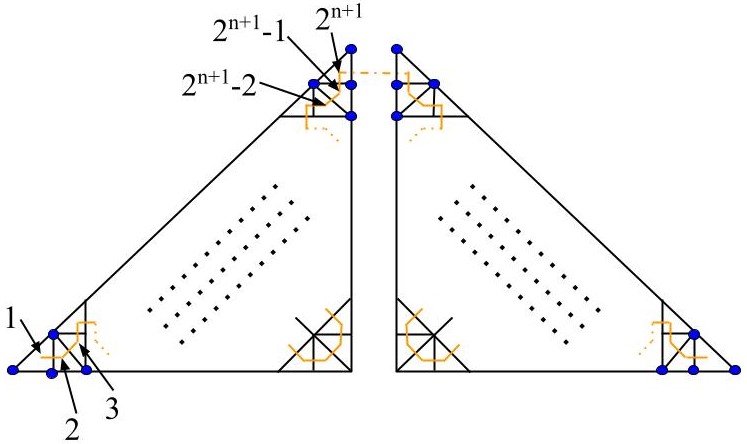
Using mathematical induction. Lemma holds for . Using fractal nature of the Sierpinski curve, iteration (even) Sierpinski curve can be constructed using two iteration Sierpinski curves, and interestingly lemma holds in both cases (See figure 7). Similar argument holds for (odd) as well. Therefore, the lemma holds.
Lemma 3
Using the evasive strategies enlisted in Table 1, a search agent can evade any obstacle lying entirely inside a single triangular cell, except when the obstacle is present inside the one of first 3 or last 3 triangular cells of GSc.
Table 1 lists evasive techniques for nodes with tags , and . The tags are given to geometries of cases 1 to 5 (refer figure 6). Cases 1-5 are the only possible geometries of three consecutive triangular cells in GSc, as proved in lemma 1. So, it remains to be shown that strategies enlisted in table 1 are always possible for each tag. Hence, the following cases :
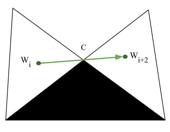
-
1.
Tag (See figure 8) : This will be impossible if lies on the boundary. Assuming lies on the boundary, there would be two line segments originating from with an interior angle , which is infeasible. Hence will never lie on the boundary. Therefore, the evasive strategy for this case will always be possible.
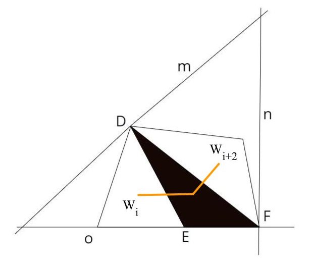
Figure 9: Tag geometry; Obstacle represented by black triangular cell -
2.
Tag (See figure 9) : Let the cell with the obstacle be denoted as . The possible boundary lines which can stop the search agent from following the evasive maneuvers are labeled as , , and .
Firstly, assume only lines and are present. Then the cell preceding will have all of its vertices on the boundary, and hence it will be either or cell from start or end (from lemma 2), which implies will be or cell; this contradicts the assumption that the cell with an obstacle is not one of the first or last three cells in GSc.
Secondly, assume only lines and are present. In this situation, the robotic system can follow the evasive strategy 2.
Thirdly, assume only lines and are present. Here, and the succeeding triangle share two vertices that lie on the boundary. This implies is either the or cell from start or end (from lemma 2). Therefore, a contradiction.
Lastly, assuming the presence of all lines , , and will imply that is the triangle from start or end (from lemma 2). Again, a contradiction.
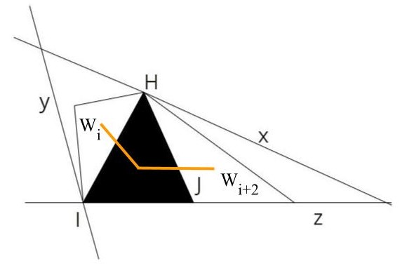
Figure 10: Tag geometry; Obstacle represented by black triangular cell -
3.
Tag (See figure 10) : Proceeding on the same lines, Let the cell with the obstacle be denoted as . The possible boundary lines which can stop the search agent from doing an evasive maneuver are labeled as , , and .
Firstly, assume only lines and are present. The cell succeeding will have all of its vertices on the boundary, and hence it will be either or cell from start or end (from lemma 2), hence will be or cell. A contradiction.
Secondly, assume only lines and are present. In this situation, the robotic system can follow evasive strategy no. 4.
Thirdly, assume only lines and are present. Here, and the preceding cell share two vertices which lie on the boundary. Which implies is either or triangle from start or end (from lemma 2). Therefore, a contradiction. Lastly, assuming the presence of all lines , , and will imply that is cell from start or end (from lemma 2). Again, a contradiction.
Therefore, The lemma is proved.
4 Multiple Obstacle Scenario
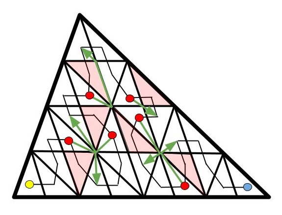
The strategy presented can be extended to situations wherein multiple obstacles are present. The alternate path for evading a single obstacle depends only on the triangular cells preceding and after the triangle with an obstacle. So, if the triangular cell has an obstacle, then the strategy presented will not work if the triangle also has an obstacle. Nevertheless, the strategy can be applied in a usual way if the triangle has an obstacle. So, the strategy will work for any number of disjoint obstacles. This is shown in figure 11.
5 Implementation & Non-Uniform Coverage Scenario
5.1 Real-life Implementation
Sierpinski curve explores a triangle, but in real life, the region to be explored may not be a triangle. It will be a closed curve. A closed region can be approximated by polygon (referred to as ) using fast and efficient algorithms; see Sklansky and Gonzalez (1980). can be triangulated to get , using existing methods with time complexity of for Siedel’s method (Seidel (1991)), for Toussaint’s method (Toussaint (1984)), and many more. The choice of method for triangulation rests with the user.
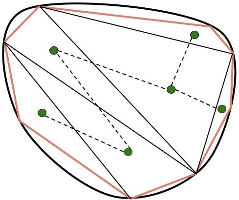
A dual graph of is generated. A dual graph of a triangulated polygon is a graph with vertices for triangles, and the vertices denoting triangles sharing sides are joined using edges (Berg et al. (1997)). Lastly, exploring the entire region will need the search agent to visit vertices of and use the Sierpinski curve to explore the triangles denoted by vertices. Traversing between the vertices of will be a Traveling Salesman Problem, whose solution can be found offline (see Figure 12).
The aerial survey of a scalene triangle using the Sierpinski curve requires function , which goes to zero on the edges, and is non-zero everywhere. can be formulated by multiplying line equations of edges of the triangle. Function ensures that the robotic system does not cross the boundary and go out of the region to be explored. Assuming the search agent at the triangular cell, and obstacle is detected at triangular cell. Using , algorithm 5.1 gives a path to be followed to triangular cell.
Algorithm for online implementation
5.2 Non-Uniform Coverage
In robotic exploration scenarios, the search agent may have some prior knowledge about the region. Search agent may be aware of certain parts of the region that have a higher probability of discovering entities of interest like minerals or resources. In such a situation, it is wise for the search agent to explore the higher probability parts rigorously, giving those parts more time and surveying them more closing. Such scenarios are referred to as Non-Uniform Coverage Planning.
Sadat et al. (2014) discusses non-uniform coverage scenarios in aerial survey. Sadat et al. (2015) go a step forward and use Hilbert’s space filling curve for exploration. Finally, with Hilbert’s space-filling curve, Nair et al. (2017) introduced strategies for obstacle evasion in a non-uniform coverage context.
This paper investigates obstacle evasion for the Sierpinski curve in non-uniform scenarios using strategy presented in Section 3. The parts of the region which are required to be explored rigorously are traversed using a higher iteration Sierpinski curve, Which allows the aerial vehicle to spend more time on such parts. Nevertheless, the distance between surface of the region and the aerial vehicle reduces as sensing radius is reduced, implying lesser loss of information due to errors.

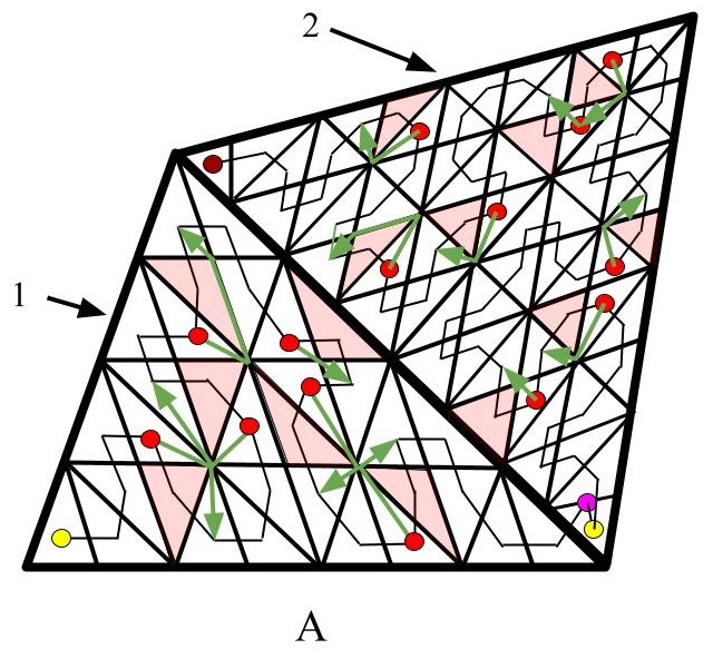
Here, we use Shortcut Heuristic (denoted as SH) for traveling between parts (see Sadat et al. (2014)). In SH, a search agent visits all the triangular cells at the lowest level of a part, then visits the nearest triangular cell of the next part and goes on visiting all the triangular cells at the lowest level in that part; this is done recursively to cover the entire region (See figure 13). Finally, figure 14 shows an example of non-uniform coverage using the Sierpinski curve.
6 Conclusion
The Aerial Survey problem using the Sierpinski curve has been considered. Strategies to evade obstacles online were presented. Simple geometric properties were used to devise evasive strategies. The suggested strategies introduced are proven to be exhaustive. The evasion plan is also shown to be helpful in non-uniform coverage situations. The strategy can be used for two or more disjoint obstacles covering triangular cells of the Sierpinski curve. The presented strategy cannot be used for obstacles covering two or more arbitrary triangular cells, but this can be a good starting point. Hence further work demands consideration of arbitrary sized and shaped obstacles.
References
- Bader (2012) Bader, M. (2012). Space-filling curves: an introduction with applications in scientific computing, volume 9. Springer Science & Business Media.
- Ban et al. (2013) Ban, X., Goswami, M., Zeng, W., Gu, X., and Gao, J. (2013). Topology dependent space filling curves for sensor networks and applications. In 2013 Proceedings IEEE INFOCOM, 2166–2174. IEEE.
- Berg et al. (1997) Berg, M.d., Kreveld, M.v., Overmars, M., and Schwarzkopf, O. (1997). Computational geometry. In Computational geometry, 1–17. Springer.
- Dafner et al. (2000) Dafner, R., Cohen-Or, D., and Matias, Y. (2000). Context-based space filling curves. In Computer Graphics Forum, volume 19, 209–218. Wiley Online Library.
- Galceran and Carreras (2013) Galceran, E. and Carreras, M. (2013). A survey on coverage path planning for robotics. Robotics and Autonomous systems, 61(12), 1258–1276.
- Joshi et al. (2019) Joshi, A.A., Bhatt, M.C., and Sinha, A. (2019). Modification of hilbert’s space-filling curve to avoid obstacles: A robotic path-planning strategy. In 2019 Sixth Indian Control Conference (ICC), 338–343. IEEE.
- Kanatani et al. (2016) Kanatani, K., Sugaya, Y., and Kanazawa, Y. (2016). Guide to 3D Vision Computation, volume 3. Springer.
- Memon et al. (2000) Memon, N., Neuhoff, D.L., and Shende, S. (2000). An analysis of some common scanning techniques for lossless image coding. IEEE transactions on image processing, 9(11), 1837–1848.
- Nair et al. (2017) Nair, S.H., Sinha, A., and Vachhani, L. (2017). Hilbert’s space-filling curve for regions with holes. In 2017 IEEE 56th annual Conference on decision and control (CDC), 313–319. IEEE.
- Sadat et al. (2015) Sadat, S.A., Wawerla, J., and Vaughan, R. (2015). Fractal trajectories for online non-uniform aerial coverage. In 2015 IEEE international conference on robotics and automation (ICRA), 2971–2976. IEEE.
- Sadat et al. (2014) Sadat, S.A., Wawerla, J., and Vaughan, R.T. (2014). Recursive non-uniform coverage of unknown terrains for uavs. In 2014 IEEE/RSJ International Conference on Intelligent Robots and Systems, 1742–1747. IEEE.
- Sagan (1994) Sagan, H. (1994). Hilbert’s space-filling curve. In Space-filling curves, 9–30. Springer.
- Seidel (1991) Seidel, R. (1991). A simple and fast incremental randomized algorithm for computing trapezoidal decompositions and for triangulating polygons. Computational Geometry, 1(1), 51–64.
- Sklansky and Gonzalez (1980) Sklansky, J. and Gonzalez, V. (1980). Fast polygonal approximation of digitized curves. Pattern recognition, 12(5), 327–331.
- Spires and Goldsmith (1998) Spires, S.V. and Goldsmith, S.Y. (1998). Exhaustive geographic search with mobile robots along space-filling curves. In International Workshop on Collective Robotics, 1–12. Springer.
- Tiwari et al. (2007) Tiwari, A., Chandra, H., Yadegar, J., and Wang, J. (2007). Constructing optimal cyclic tours for planar exploration and obstacle avoidance: A graph theory approach. In Advances in Cooperative Control and Optimization, 145–165. Springer.
- Toussaint (1984) Toussaint, G.T. (1984). A new linear algorithm for triangulating monotone polygons. Pattern Recognition Letters, 2(3), 155–158.
- Zumbusch (2000) Zumbusch, G. (2000). On the quality of space-filling curve induced partitions. Citeseer.