Closed-Loop View of the Regulation of AI:
Equal Impact across Repeated Interactions

Abstract

There has been much recent interest in the regulation of AI. We argue for a view based on civil-rights legislation, built on the notions of equal treatment and equal impact. In a closed-loop view of the AI system and its users, the equal treatment concerns one pass through the loop. Equal impact, in our view, concerns the long-run average behaviour across repeated interactions. In order to establish the existence of the average and its properties, one needs to study the ergodic properties of the closed-loop and, in particular, its unique stationary measure.

Introduction

There has been considerable interest in the regulation of artificial intelligence (AI), recently. It is increasingly recognized that so-called high-risk applications of AI, such as in Human Resources, Retail Banking, or within public schools, be it admissions or assessment, cannot be served by black-box AI systems with no human control. It is not clear [10], however, how to phrase even the desiderata for the regulation of AI.

Here, we suggest that the desiderata could be the same as in the Civil Rights Act of 1964 and much of the subsequent civil-right legislation world-wide: equal treatment and equal impact. At the same time, we point out that these desiderata could be in conflict [34].

Let us illustrate the conflict on an example of a system that performs credit-risk estimate in a consumer-credit company. In the US, this is regulated by the Equal Credit Opportunity Act of 1974, but the example applies equally well to other countries. Let us imagine a situation, where the the credit decision is uniform: Everyone who has not defaulted on any loan is approved a credit up to $50000. Anyone else is declined credit. This is clearly the most “equal treatment” possible, in the spirit of non-discrimination “on the basis of race, color, religion, national origin, sex, marital status, age, receipt of public assistance”, as mandated by the Equal Credit Opportunity Act. At the same time, if one subgroup (defined by whichever protected attribute, e.g., race or the receipt of public assistance) is having a lower-than-average income, its default rate on the $50000 loan may be higher than of the other subgroup. Over time, the subgroup with lower-than-average income will be regularly declined credit as a result of these defaults, in violation of the “equal impact”. On the other hand, if the credit limit is, e.g., set at three times the annual salary, the subgroup with lower-than-average income will be offered lower credit limits, in violation of the “equal treatment”. The differentiated credit limits may make it possible for the same subgroup to repay the loans successfully, though, to develop a credit history, and eventually lead to a positive and “equal impact”. See the penultimate section of this paper for further details of the application.

Our original contribution then stems from the reinterpreting of the meaning of equal treatment and equal impact within a closed-loop view of the AI system. There, the AI system produces information, which is communicated to the users, who respond to the information. The aggregate actions of the users are observed and serve as an input to further uses of the AI systems. Equal treatment concerns a single run of this closed loop, while equal impact concerns long-run properties of this closed loop.

The a closed-loop view of the AI system addresses several important shortcomings of presently proposed systems:

• it very clearly distinguishes equal impact from equal treatment

• it allows for a stochastic response of the users to the information produced by the AI system, rather than assuming it is deterministic

• it explicitly models the “concept drift” and retraining of the AI systems over time, inherent in practical AI systems, but ignored by most analyses of AI systems.

In terms of technical results, we formalise the notions above, present one condition that is necessary for the equal impact of an AI system, and illustrate the notions on the credit-risk use case.

Related Work

Regulation of AI

While there is a long history of research on the interface of AI and law [3, 19, 4, e.g.], much recent interest [27, 21, e.g.] has been sparked by the plans to introduce AI regulation within the legal system. Arguably, the European Commission regulates AI already: Article 22.1 of the General Data Protection Regulation (GDPR) is sometimes interpreted as prohibiting fully automated decisions with legal effect or “similarly significant effect”. There is much discussions regarding the AI Act [29] in the Europe Union, and the potential extensions of the regulatory framework in the USA [7].

Within the recent discussions, a fair amount of attention focuses on the question of defining AI [24] – or whether one should like to regulate the use of any algorithm [23, 11] – and defining high-risk uses of AI. One would also like to distinguish [26] between the harm of the individual and the society.

In contrast, we distinguish between the treatment within a single interaction with the AI system and the impact of the repeated interactions with the AI system.

Control Theory

Our approach is rooted in the closed-loop view of feedback control, but with several important differences:

To begin, conventional control is usually focused on regulating a single system. The system achieves the required behaviour most efficiently given the restrictions imposed by the challenge and the available resources. Even in areas where large-scale coupled systems are studied, the behaviour of all system components is analyzed and developed. On the other hand, in artificial intelligence, it is not the behaviour of individual users that is of interest. Rather than that, the variable of interest is the aggregate impact of the acts of a large number of users. Synchronizing behaviours is unneeded, if not detrimental because it is not even essential for all users to act rationally. Examples of this kind of analysis include demand management for shared resources such as water and electricity, and the provision of medical care. De-synchronization alleviates the supply strain, and collective effects quantify the supply’s quality. On the other hand, limits on the needed level of service for persons vary according to the application area.

Second, classical control, in general, is concerned with the control of systems with fixed dimensions. On the other hand, artificial intelligence often regulates and affect the behaviour of large-scale populations. Even the system’s dimension may be unpredictable and variable in such settings, emphasizing the critical requirement for scale-free management of extremely large-scale systems. Except in the case of passive control design, scale-free control for large systems is a largely unexplored issue in the classical control field.

Thirdly, in classical control, the controlled system’s mathematical description does not change in response to control signals. This underlying concept is challenging to realize in artificial intelligence. By and large, models can only approximate the dynamics of the actual systems. This is not an issue as long as there is an appreciation for the possibility of reality and model deviating from one other. However, models in artificial intelligence are not easily derived from first principles; instead, they are empirical, i.e., based on data gathered from measurements of existing processes. Additionally, controlled studies cannot gather empirical data across a variety of operating points but must be obtained directly from the system.

An effort to enhance the processes above, for example, by sending information to the users involved, establishes a feedback loop that did not exist earlier. This change in the underlying process may invalidate the empirical model since there were no data available to represent the dynamic influence of such feedback during the model’s development. Frequently, offered solutions ignore this feedback loop. This latter aspect necessitates a far more extensive examination of prediction and optimization under feedback than has hitherto been the case.

Fourth, data sets are often gathered in a closed loop in fashion like Figure 1. That is, public data sets often contain information about decision-makers. Developing models of large-scale feedback systems is a crucial hurdle to development in applying certain control methods to artificial intelligence. In dealing with such impacts, artificial intelligence researcher may have a lot to learn from economic and control theory.

Finally, and perhaps most significantly, a fundamental distinction between classical control and our approach is the need to investigate the influence of control signals on the statistical features of the populations under control. Given that we are often dealing with service delivery, these statistical features should be stationary and predictable, necessitating ergodic control design.

Control of Multi-user Dynamical Systems

Perhaps the closest to our work within control theory are multi-user dynamical systems over networks. There, the principle concern is the design of distributed protocols that provide consensus or synchronisation of states of all users [5, 20]. (The states might indicate vehicle directions or locations, estimations of sensor readings in a sensor network, oscillation frequencies, and each user’s trust opinion, among other things.) To achieve synchronised behaviour in multi-user systems, all systems must agree on the values of these quantities.

Studying their interactions and collective behaviours under the effect of the information flow permitted by the communication network is critical for networked cooperative dynamical systems. This communication network may be seen as a graph with directed edges or connections corresponding to the information travelling between the systems. The systems are portrayed as nodes on the graph and are sometimes referred to as users. In communication networks, information flows exclusively between the graph’s close neighbours. However, if a network is linked, this locally sent information eventually reaches every user in the graph.

In cooperative control systems based on graphs, there are fascinating interactions between the dynamics of the individual users and the communication graph’s topology. The graph topology may severely constrain the performance of the users’ control rules. To be precise, in cooperative control on graphs, all control protocols must be distributed so that each user’s control rule is limited to knowledge about its near neighbours in the network topology. If sufficient attention is not taken while constructing the local user control rules, the dynamics of the individual users may be stable, but the graph’s networked systems may display undesired behaviours. Due to the communication constraints imposed by graph topologies, complex and fascinating behaviours are seen in multi-user systems on graphs that are not found in single-user, centralised, or decentralised feedback control systems.

The ideas of distributed cooperative control are used in [17] to construct optimal and adaptive control systems for multi-user dynamics on graphs. The requirement complicates these designs that all control and parameter tweaking methods must be dispersed in the network to rely on just their near neighbours.

[17] analysed discrete-time systems and demonstrate that an additional condition between the local user dynamics and the graph topology must be met to ensure global synchronization when the local optimum design is used. Global optimization of collective group movements is more challenging than locally optimizing each user’s motion. A typical issue in optimum decentralized control is that global optimization problems often demand knowledge from all users, which distributed controllers cannot access since they can only utilize information from closest neighbours. Further, they demonstrate, globally optimum distributed form controls may not exist on a particular graph. To achieve globally optimum performance when employing distributed protocols that rely only on local user information in the graph, the global performance index must be chosen to depend on graph features, notably the graph Laplacian matrix. They also establish distinct global optimality for which distributed control solutions are always possible on sufficiently linked networks. There, they examine multi-user graphical games and demonstrate that a Nash equilibrium results when each user optimizes its local performance index. For more results on these direction we refer [25, 31, 30, 33, 8].

A Closed-Loop View of AI Systems

Let us consider a closed-loop model based on the following constraints:

• Users get information from the AI System, but are not required to take action based on the AI System’s outputs. It will be convenient to encode an users’ reaction to the output probabilistically.

• The AI System does not necessarily monitor individual users’ actions (“profiling”), but rather some aggregate or otherwise filtered version.

• The users do not communicate with one another, or only in response to information broadcast by the central authority.

Figure 1: A closed-loop model of an AI system and its interactions with the users: the AI system provides some outputs, e.g., scorecards in credit scoring, matches in a matching market, or suggestions in a decision-support system. Users observe the outputs and take action in response. With some delay, their actions in response to the outputs are utilized in retraining the AI System.

Ultimately, the repeated uses of an AI system can be seen as the closed loop of Figure 1. The AI System produces some outputs $\pi(k)$ at time $k$, e.g., lending decisions in financial services, matches in a two-sided market, or suggestions in a decision-support system. The output is taken up by $N$ users of the system, who have some states $x_{i}$, $i\in[N]$ internal to them, where $[N]=1,\ldots,N$.

The users take some action, which can be modelled as a probability function of the output and the private state, over the certain user-specific sets of actions. The action $y_{i}\left(k\right)$ of user $i$ at time $k$ is then a random variable. In the remainder, we will assume $y_{i}\left(k\right)$ are scalars, but generalisations are easy to obtain. The aggregate of the actions $y(k)=\sum\limits_{i=1}^{N}y_{i}\left(k\right)$ at time $k$ is then also a random variable. The AI System may not have access to either $x_{i}\left(k\right)$, $y_{i}\left(k\right)$, but perhaps only $y(k)$ or some filtered version. The filter may accumulate the data, for instance, before filtering out anomalies.

Equal Treatment

Equal treatment very clearly examines the AI system’s treatment of the user population’s and the influence on the microscopic qualities over the short run.

Definition 1 (Equal Treatment).

For each user $i$, we require that

• the system provides the same information $\pi(k)$ to all users $i$,

• that there exists a constant $\overline{r}$ such that

  $$y_{i}(j)=\overline{r},$$ (1)

  where this constant is independent of initial conditions.

Definition 2 (Equal Treatment Conditioned on Non-Protected Attributes).

For each user $i$ within a class that is defined by non-protected attributes, we require that

• the system provides the same information $\pi(k)$ to all users within the class;

• that there exists a constant $\overline{r}$ such that

  $$y_{i}(j)=\overline{r},$$ (2)

  where this constant is independent of initial conditions.

Notice that there is a sufficiently large overlap of the classes that are defined by non-protected attributes such that the definition reduces to the unconditional equal treatment.

Equal Impact

Equal impact very clearly examines the AI system’s influence on the user population’s microscopic qualities over the long run. One may desire, for example, that each user obtains a fair portion of the resource on average over time, or, at a far more fundamental level, that the average allocation of the resource to each user over time is a stable number that is predictable and independent of beginning circumstances.

To model equal impact, we construct requirements that ensure ergodicity: the presence of a single invariant measure to which the system is statistically drawn regardless of the starting circumstances.

Definition 3 (Equal Impact).

For each user $i$, we require that

• there exists a constant $\overline{r}_{i}$ such that

  $$\lim_{k\to\infty}\frac{1}{k+1}\sum_{j=0}^{k}y_{i}(j)=\overline{r}_{i},$$ (3)

  where this latter limit is independent of initial conditions;

• all the $\overline{r}_{i}$ coincide.

Definition 4 (Equal Impact Conditioned on Non-Protected Attributes).

For each user $i$ within a class that is defined by non-protected attributes, there exists a constant $\overline{r}_{i}$ such that

$$\lim_{k\to\infty}\frac{1}{k+1}\sum_{j=0}^{k}y_{i}(j)=\overline{r}_{i},$$ (4)

where this latter limit is independent of initial conditions. Furthermore, we require that all the $\overline{r}_{i}$ coincide.

Guarantees of these Properties

Proving that there is a unique invariant measure is not necessarily an easy undertaking. Even well-known AI systems do not always result in feedback systems that exhibit equal impact.

Under the assumptions of continuity of the closed loop model, the work on iterated function systems [12, 2, 9], which are a class of stochastic dynamical systems arising from the multi-user interactions, makes it possible to obtain strong stability guarantees for such stochastic systems under the assumptions of continuity of the closed loop model. The following are shown in the work [13]:

• Even if regulation is accomplished by controlling the behaviour of ensembles of users, feedback control with integral action has the potential to disrupt the closed-loop system’s ergodic features. This discovery is significant because ergodic behaviour is necessary for supporting economic contracts and ensuring the existence of attributes such as fairness. Thus, from a practical standpoint, the finding is one of the system’s critical features and is not only theoretically interesting.

• A few particular instances are given to demonstrate the loss of ergodicity in seemingly innocuous situations.

• For particular population types and filters, stable control action always results in ergodic behaviour. It was particularly shown for linear and non-linear systems with both real-valued and finite-set actions.

• Finally, a minor contribution was made to demonstrate how the results from the study of iterated function systems might be used in designing controllers for specific types of dynamic systems.

In this paper, we have to relax the continuity assumptions, however. Indeed, the classification problems involve discrete sets such as the “credit denied” or “credit approved”, which cannot be easily modelled with continuous fuctions. So in this case, stochastic, user-specific response to the feedback signal $\pi(k)\in\Pi$ can be modelled by user-specific and signal-specific probability distributions over the certain user-specific sets of actions

$$\mathbb{A}_{i}=\{a_{1},\ldots,a_{L}\}\subset\mathbb{R}^{n_{i}},$$ (5)

where $\mathbb{R}^{n_{i}}$ can be seen as the space of $i^{\text{th}}$ user’s private state space $x_{i}$. Assume that the set of possible resource demands of user $i$ is $\mathbb{D}_{i}$, where in the case that $\mathbb{D}_{i}$ is finite we denote

$$\mathbb{D}_{i}:=\{d_{i,1},d_{i,2},\ldots,d_{i,m_{i}}\}.$$ (6)

In the general case, we assume there are $\tau_{i}\in\mathbb{N}$ state transition maps

$$w_{ij}:\mathbb{R}^{n_{i}}\to\mathbb{R}^{n_{i}},j=1,\ldots,\tau_{i}$$

for user $i$ and output maps

$$w^{\prime}_{i\ell}:\mathbb{R}^{n_{i}}\to\mathbb{D}_{i},\ell=1,\ldots,\kappa_{i},\kappa_{i}\in\mathbb{N},$$

for each user $i$. The evolution of the states and the corresponding demands then satisfy:

$$x_{i}\left(k+1\right) =w_{ij}\left(x_{i}(k)\right)\;|\;j=1,\ldots,\tau_{i},$$ (7a)

$$y_{i}(k) =w^{\prime}_{i\ell}\left(x_{i}(k)\right)\;|\;\ell=1,\ldots,\kappa_{i},$$ (7b)

where the choice of user $i$’s response at time $k$ is governed by probability functions

$$p_{ij}:\Pi\to[0,1],j=1,\ldots,\tau_{i}$$ (8a)

$$p^{\prime}_{i\ell}:\Pi\to[0,1],\ell=1,\ldots,\kappa_{i},$$ (8b)

respectively. Specifically, for each user $i$, for all $k\in\mathbb{N}$ and for all signal $\pi$ we have that:

$$\mathbb{P}\big{(}x_{i}\left(k+1\right)=w_{ij}\left(x_{i}(k)\right)\big{)}=p_{ij}\left(\pi(k)\right),$$ (9a)

$$\mathbb{P}\big{(}y_{i}(k)=w^{\prime}_{i\ell}\left(x_{i}(k)\right)\big{)}=p^{\prime}_{i\ell}\left(\pi(k)\right),$$ (9b)

$$\sum\limits_{j=1}^{\tau_{i}}p_{ij}\left(\pi\right)=\sum\limits_{\ell=1}^{\kappa_{i}}p^{\prime}_{i\ell}\left(\pi\right)=1.$$ (9c)

Then, one can prove that when the graph $G=(X,E)$ is strongly connected, there exists an invariant measure for the feedback loop. If in addition, the adjacency matrix of the graph is primitive, then the invariant measure is attractive and the system is uniquely ergodic.

For linear systems, this is a direct consequence of (Werner, 2004) and the observation that the necessary contractivity properties follow from the internal asymptotic stability of controller and filter. For non-linear systems, similar results can be obtained using [18, Theorem 2]. See also [14] and the Supplementary information.

Numerical Illustrations

Credit scoring refers to the process of lenders, usually financial institutions, measuring the creditworthiness of a person or a small business. In USA, Equal Credit Opportunity Act (ECOA) and the part of the law that defines its authority and scope, known as Regulation B, require statements of specific reasons for adverse credit decisions, where it would be difficult, yet impossible to comply if complex algorithms or “black-box” models are used. Instead, scorecards are commonly adopted in practice, due to their explainability. Table 1 displays a simple scorecard.

Factor	Code	Description	Score
History	-	$\times$ Average Default Rate	-8.17
Income	0	$\leq\$15\textrm{K}$	0
	1	$>\$15\textrm{K}$	+5.77

Table 1: A simple scorecard for existing users. For example, an user with annual income $\$50\textrm{K}$ and an average default rate $0.1$ would be given a score of $-8.17\times 0.1+5.77=4.953$.

Although Table 1 might seem fair at first sight, income is a factor closely related to protected attributes, e.g., race. Figure 2 displays the 2020 annual income distribution of households by race, including “BLACK ALONE” (blue), “WHITE ALONE” (pink) and “ASIAN ALONE” (green), in the USA, sourced from Table A-2. Households by Total Money Income, Race, and Hispanic Origin of Householder: 1967 to 2020 (Table A-2), from US Census Bureau . The green bar on the index “over 200” implied that a larger share (almost 20%) of “ASIAN ALONE” households makes more than $\$200\textrm{K}$ in 2020. On the other hand, the income of most “BLACK ALONE” households is less than $\$75\textrm{K}$. This figure casts doubt on the equal treatment using the scorecard in Table 1, because races with generally lower incomes would receive a lower credit score. If a lender tries to maintain similar credit distributions across different races, the results may not be as expected in the long run, as low-income households might end up defaulting or even not be able to apply for another mortgage ever after.

Figure 2: The 2020 annual income distribution of “BLACK ALONE”, “WHITE ALONE” and “ASIAN ALONE” households in USA, with three races distinguished by colours. Data are sourced from Table A-2 of the Current Population Survey (CPS) of US Census Bureau.

Our notion of equal impact in the context of credit scoring would equalise the long-term average default rate across races or across individuals, such that low-income households can keep better credit history. Recall Figure 1 from the perspective of credit scoring. Given the goal of equal impact, at each time step, the income $z_{i}(k)$ is internal to the user (user), while her income code $\mathbbm{1}_{\geq 15}z_{i}(k)$ is visible to a lender, where $\mathbbm{1}_{\geq 15}$ is an indicator function that maps the input to one if $\geq 15$ is satisfied and all other values to zero. The lender would use the AI system, i.e., logistic regression in our case, to build a scorecard and reveal a credit decision $\pi(k,i)$ (e.g., approval or denial of a mortgage transaction) to user $i$ at time $k$. Note that the scorecard only gives a credit score, but, based on a cut-off score, the lender is able to reach a credit decision. Confidential to cilent $i$, her state $x_{i}(k)$ at time $k$ is determined by her income and, in turn, influences the repayment action. Its repayment action $y_{i}(k)\in\{0,1\}$ is modelled as a Gaussian conditional independence model [28, 16, 22]. Afterwards, the filter calculates the average default rates of each user, using historical repayment actions $y_{i}(k)$ for $i\in 0,\ldots,k$. The average default rates, along with the income code of users, would be used as training data for the AI system, and further, new credit decisions $\pi(k+1,i),i\in[N]$ are made again using logistic regression.

For the numerical experiments, we use the real-world data from Table A-2, which gives the number of households and income distribution by year and race. We consider a period from 2002 to 2020, with a year being a time step, because in 2002 the Annual Social and Economic Supplement (ASEC) of the Current Population Survey (CPS) started to allow households to report their race from more diverse options. Let $\mathcal{S}$ be a set that includes 3 races: “BLACK ALONE”, “WHITE ALONE” and “ASIAN ALONE”. In the beginning of 2002 (time $0$), we generate $N=1000$ users (households), whose races are sampled from $\mathcal{S}$ with a distribution of $[0.1235,0.8406,0.0359]$. Notice that the distribution is the ratio of the number of households of the three races in 2002 in Table A-2. The generated user set is then divided into 3 subsets according to race, denoted by $\mathcal{N}_{s}$, for $s\in\mathcal{S}$. Further, following the income distribution of the year $2002+k$ and race $s$, we sample the income $z_{i}(k)$ of user $i\in\mathcal{N}_{s}$ at time $k$.

For simplicity, we assume that $\pi_{i}(k,i)=1$ denotes that user $i$ is offered a 3.5-times-income mortgage at time $k$. Assuming that the annual mortgage rate and the basic living cost are 2.16% per annum and $\$10\textrm{K}$, we use the Gaussian conditional independence model [22] to generate the repayment actions. Suppose that the state $x_{i}(k)$ measures the portion of income left after deduction of living cost and mortgage interest:

$$x_{i}(k)=\frac{z_{i}(k)-10-3.5\times 2.16\%\times z_{i}(k)}{z_{i}(k)}.$$ (10)

The binary repayment action $y_{i}(k)$ (1 for repaid) is defined by (11).

$$\begin{cases}y_{i}(k)=0&\begin{split}&\text{for }x_{i}(k)\leq 0\\ &\;\text{ or }\pi(k,i)=0,\end{split}\\ y_{i}(k)\sim\textrm{Bernoulli}\left(F\left(5\times x_{i}(k)\right)\right)&\text{otherwise, }\end{cases}$$ (11)

where user $i$ would not make a repayment if no mortgage is offered or if her income cannot cover the basic living cost plus mortgage interest. Otherwise, the repayment action follows a Bernoulli distribution with $\textrm{Pr}(y_{i}(k)=1)=F(5\times x_{i}(k))$, where $F(\cdot)$ is the cumulative distribution function of the standard normal distribution.

Furthermore, we define default as a mortgage offered but not repaid, i.e., $y_{i}(k)=0|\;\pi(k,i)=1$. We introduce the average default rate $\textrm{ADR}_{i}(k)$ for user $i$ and the race-wise version $\textrm{ADR}_{s}(k)$ for race $s$ at time $k$, as defined in (12):

$$\begin{split}\textrm{ADR}_{i}(k):=&\textrm{Pr}(y_{i}(k)=0|\pi(k,i)=1)\\ =&1-\sum_{j=0}^{k}\frac{y_{i}(j)}{\pi(k,i)}\\ \textrm{ADR}_{s}(k):=&\textrm{Pr}(y_{i}(k)=0|\pi(k,i)=1,i\in\mathcal{N}_{s})\\ =&1-\frac{1}{|\mathcal{N}_{s}|}\sum_{i\in\mathcal{N}_{s}}\sum_{j=0}^{k}\frac{y_{i}(j)}{\pi(k,i)},\end{split}$$ (12)

where $|\mathcal{N}_{s}|$ denotes the number of users of race $s$. With the goal of equal impact, we wish to equalise the outcome of credit scoring among individuals in the long run, such that

$$\lim_{k\to\infty}\textrm{ADR}_{i}(k)=\overline{r}_{i},\quad\lim_{k\to\infty}\textrm{ADR}_{s}(k)=\overline{r}_{s},$$ (13)

and that all $\overline{r}_{i}$ coincide and all $\overline{r}_{s}$ coincide.

Figure 3: Solid curves depict the mean value of time series $\{\textrm{ADR}_{s}(k)\}_{k\in[N]}$, across 5 trials, for all races. Error shades display mean $\pm$ one standard deviation.

Figure 4: The time series $\{\textrm{ADR}_{i}(k)\}_{k\in[N]}$ for all users from 5 trials ($5\times 1000$ curves), with their races distinguished by colour.

Figure 5: The density of ADR${}_{i}(k)$ at different time steps, with the race information ignored.

For the year of 2002-2003 (time 0 & 1), no scorecard is used and we assume all users are given the approval of the mortgage, e.g., $\pi(k,i):=1$, for $i\in[N]$ and $k=\{0,1\}$. Thus, we obtain the initilisation of average default rates, i.e., $\textrm{ADR}_{i}(0),\textrm{ADR}_{s}(0)$ and $\textrm{ADR}_{i}(1),\textrm{ADR}_{s}(1)$. Afterwards, for time $k\geq 2$, a scorecard is built, whose parameters are trained from a logistic model, with independent variables being $\mathbbm{1}_{\geq 15}z_{i}(k)$, ADR${}_{i}(k-1)$ and the dependent variable being $\ln{\frac{y_{i}(k)}{1-y_{i}(k)}}$. Although, the scorecard $\pi(k)$ can vary in time steps, we use the same cut-off score 0.4 to decide each user’s credit decision (0 for denial and 1 for approval). Using our notation, the example of Table 1 would be rewritten as

$$\begin{split}&-8.17\times\textrm{ADR}_{i}(k-1)+5.77\times\mathbbm{1}_{\geq 15}z_{i}(k)=4.953\\ &\qquad\quad\Rightarrow\quad 4.953>0.4\quad\Rightarrow\quad\pi(k,i)=1.\end{split}$$

We define a trial as the simulation of generating 1000 users and repeating the closed-loop for the period 2002-2020. In our numerical experiments, 5 trials are conducted, with each trial using a new batch of 1000 users. For consistency with previous figures, “BLACK ALONE”, “WHITE ALONE”, and “ASIAN ALONE” subgroups are represented by blue, pink and green, respectively. Notice that the sequence of $\{\textrm{ADR}_{i}(k)\}_{k\in[N]}$ for an user $i$, and that of $\{\textrm{ADR}_{s}(k)\}_{k\in[N]}$ for a race $s$, could be seen as time series. Recall the goal of equal impact in (13), we would like to see these time series converge (weakly to the same distribution).

Figure 4 presents the mean value of the time series $\{\textrm{ADR}_{s}(k)\}_{k\in[N]}$ across 5 trials, by solid curves and $\pm$ one standard deviation by error shades. Figure 4 displays the time series $\{\textrm{ADR}_{i}(k)\}_{k\in[N]}$ for all users from 5 trials ($5\times 1000$ curves), with their races distinguished by colour. In Figure 5, the race information is ignored, and the grey shading shows the density of ADR${}_{i}(k)$ at different time steps.

Conclusions

We have presented a novel, closed-loop view of the impact of AI systems. On an example in consumer-credit approvals, we showcase, that equal impact is possible while preserving equal treatment conditional on a non-protected attribute of income. An important question for further work is how to impose constraints on the equality of impact [6]. Another important question asks whether the coupling arguments of Hairer et al. [15] could make it possible to show certain contrapositive statements, suggesting when such guarantees are impossible to provide.

Markov Systems

A Markov system (see Figure 6) is a family $\left(X_{i(e)},w_{e},p_{e}\right)_{e\in E}$ where $E$ consisting of edges of a finite directed (multi) graph $\left(V,E,i,t\right)$ with $V=\{1,2,\dots,N\}$ are vertices and $N=1$ is also possible, $i:E\to V$ indicates the initial vertex of each edge and $t:E\to V$ indicates the terminal vertex of each edge, $X_{1},\dots,X_{N}$ is a partition of the metric space $(X,d)$ into non-empty Borel subsets, $\left(w_{e}\right)_{e\in E}$ is a family of Borel-measurable maps on the metric space such that

$$w\left(X_{i(e)}\right)\subseteq X_{t(e)}\;\text{for all }e\in E,$$

and $\left(p_{e}\right)_{e\in E}$ is a family of Borel measurable maps on $X$ with the property $p_{e}(x)\geq 0$ for all $e\in E$ and $\sum\limits_{e\in E}p_{e}(x)=1$  for all $x\in X$. A Markov system is called irreducible or aperiodic if its directed graph is irreducible or aperiodic. A Markov system is called contractive with contraction factor $a$ if its probability functions satisfy the following average contractivity condition, $\text{for all }x,y\in X_{i},\;i=1,2,\dots,N$,

$$\sum\limits_{e\in E}p_{e}(x)d(w_{e}(x),w_{e}(y))\leq ad(x,y).$$

The Markov system defined above determines a Markov operator $\mathrm{P}$ on the space of bounded Borel measurable functions on $X$, which is denoted by $\mathcal{L}^{0}(X)$,

$$\mathrm{P}f(x)=\sum\limits_{e\in E}p_{e}f\circ w_{e}\;\text{ for all }f\in\mathcal{L}^{0}(X),$$

and the adjoint of $\mathrm{P}$ is denoted by $\mathrm{P}^{\star}$ acts on the space of Borel probability measures $\mathcal{M}_{p}(X)$ as

$$\mathrm{P}^{\star}\nu(f)=\int\mathrm{P}(f)\mathrm{d}\nu\;\text{for all }\nu\in\mathcal{M}_{p}(X).$$

A Borel probability measure $\mu$ is said to be an invariant probability measure for the Markov system if it is a stationary distribution of the associated Markov process i.e.

$$\mathrm{P}^{\star}\mu=\mu.$$

A Borel probability measure $\mu$ is called attractive for the contractive Markov system iff

$$\lim_{n\to\infty}(\mathrm{P}^{\star})^{n}\nu\to\mu\;\text{ for all }\nu\in\mathcal{M}_{p}(X).$$

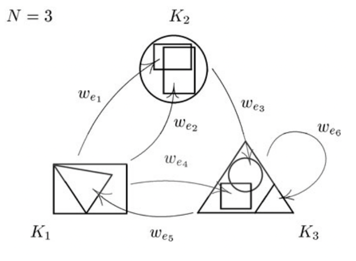
Figure 6: A Markov system [32]

Incremental Stability

Incremental stability is a well-established concept to describe the asymptotic property of differences between any two solutions. One can utilise the concept of incremental input-to-state stability, which is defined as follows:

Definition 5.

A function $\gamma:\mathbb{R}^{+}\to\mathbb{R}^{+}$ is is said to be of class $\mathcal{K}$ if it is continuous, increasing and $\gamma(0)=0$. It is of class $\mathcal{K}_{\infty}$ if, in addition, it is proper, i.e., unbounded.

Definition 6.

A continuous function $\beta:\mathbb{R}^{+}\times\mathbb{R}^{+}\to\mathbb{R}^{+}$ is said to be of class $\mathcal{K}\mathcal{L}$, if for all fixed $t$ the function $\beta(\cdot,t)$ is of class $\mathcal{K}$ and for all fixed $s$, the function $\beta(s,\cdot)$ is is non-increasing and tends to zero as $t\to\infty$.

Definition 7 (Incremental ISS, [1]).

Let $\mathcal{U}$ denote the set of all input functions $u:\mathbb{Z}_{\geq k_{0}}\to\mathbb{R}^{d}$ Suppose $F:\mathbb{R}^{d}\times\mathbb{R}^{n}\to\mathbb{R}^{n}$ is continuous, then the discrete-time non-linear dynamical system

$$x(k+1)=F(x(k),u(k)),$$ (14)

is called (globally) incrementally input-to-state-stable (incrementally ISS), if there exist $\beta\in\mathcal{KL}$ and $\gamma\in\mathcal{K}$ such that for any pair of inputs $u_{1},u_{1}\in\mathcal{U}$ and any pair of initial condition $\xi_{1},\xi_{2}\in\mathbb{R}^{n}$:

$$\|x(k,\xi_{1},u_{1})-x(k,\xi_{2},u_{2})\|\leq\beta(\|\xi_{1}-\xi_{2}\|,k)+$$

$$\gamma(\|u_{1}-u_{2}\|_{\infty}),\quad\forall k\in\mathbb{N}.$$

References

- [1] David Angeli. A Lyapunov approach to incremental stability properties. IEEE Transactions on Automatic Control, 47(3):410–421, 2002.
- [2] Michael F Barnsley, John H Elton, and Douglas P Hardin. Recurrent iterated function systems. Constructive approximation, 5(1):3–31, 1989.
- [3] Trevor Bench-Capon, Michał Araszkiewicz, Kevin Ashley, Katie Atkinson, Floris Bex, Filipe Borges, Daniele Bourcier, Paul Bourgine, Jack G Conrad, Enrico Francesconi, et al. A history of ai and law in 50 papers: 25 years of the international conference on ai and law. Artificial Intelligence and Law, 20(3):215–319, 2012.
- [4] Nicholas Berente, Bin Gu, Jan Recker, and Radhika Santhanam. Managing artificial intelligence. MIS quarterly, 45(3):1433–1450, 2021.
- [5] Vincent D Blondel, Julien M Hendrickx, Alex Olshevsky, and John N Tsitsiklis. Convergence in multiagent coordination, consensus, and flocking. In Proceedings of the 44th IEEE Conference on Decision and Control, pages 2996–3000. IEEE, 2005.
- [6] L Elisa Celis, Lingxiao Huang, Vijay Keswani, and Nisheeth K Vishnoi. Classification with fairness constraints: A meta-algorithm with provable guarantees. In Proceedings of the conference on fairness, accountability, and transparency, pages 319–328, 2019.
- [7] Yoon Chae. Us ai regulation guide: legislative overview and practical considerations. The Journal of Robotics, Artificial Intelligence & Law, 3, 2020.
- [8] Fei Chen, Wei Ren, et al. On the control of multi-agent systems: A survey. Foundations and Trends® in Systems and Control, 6(4):339–499, 2019.
- [9] P. Diaconis and D. Freedman. Iterated random functions. SIAM Review, 41(1):45–76, 1999.
- [10] Roel Dobbe, Thomas Krendl Gilbert, and Yonatan Mintz. Hard choices in artificial intelligence. Artificial Intelligence, 300:103555, 2021.
- [11] Joshua Ellul. Should we regulate artificial intelligence or some uses of software? Discover Artificial Intelligence, 2(1):1–6, 2022.
- [12] John H Elton. An ergodic theorem for iterated maps. Ergodic Theory and Dynamical Systems, 7(04):481–488, 1987.
- [13] A. R. Fioravanti, Jakub Marecek, Robert N. Shorten, Matheus Souza, and Fabian Wirth. On the ergodic control of ensembles. Automatica, 108:108483, 2019.
- [14] Ramen Ghosh, Vyacheslav Kungurtsev, Jakub Marecek, and Robert N Shorten. On the ergodic control of ensembles in the presence of non-linear filters. arXiv preprint arXiv:2112.06767, 2021.
- [15] Martin Hairer, Jonathan C Mattingly, and Michael Scheutzow. Asymptotic coupling and a general form of harris’ theorem with applications to stochastic delay equations. Probability theory and related fields, 149(1-2):223–259, 2011.
- [16] Álvaro Leitao and Luis Ortiz-Gracia. Model-free computation of risk contributions in credit portfolios. Applied Mathematics and Computation, 382:125351, 2020.
- [17] Frank L Lewis, Hongwei Zhang, Kristian Hengster-Movric, and Abhijit Das. Cooperative control of multi-agent systems: optimal and adaptive design approaches. Springer Science & Business Media, 2013.
- [18] Jakub Marecek, Michal Roubalik, Ramen Ghosh, Robert N Shorten, and Fabian Wirth. Predictability and fairness in load aggregation and operations of virtual power plants. Automatica, 2022. arXiv preprint arXiv:2110.03001.
- [19] Arvind Narayanan. Translation tutorial: 21 fairness definitions and their politics. In Proc. Conf. Fairness Accountability Transp., New York, USA, volume 1170, page 3, 2018.
- [20] Angelia Nedic and Asuman Ozdaglar. Distributed subgradient methods for multi-agent optimization. IEEE Transactions on Automatic Control, 54(1):48–61, 2009.
- [21] Nicolas Petit and Jerome De Cooman. Models of Law and Regulation for AI. Routledge, 2021.
- [22] Marek Rutkowski and Silvio Tarca. Regulatory capital modeling for credit risk. International Journal of Theoretical and Applied Finance, 18(05):1550034, 2015.
- [23] Jonas Schuett. Defining the scope of ai regulations. arXiv preprint arXiv:1909.01095, 2019.
- [24] Jonas Schuett et al. A legal definition of ai. arXiv preprint arXiv:1909.01095, 2019.
- [25] Jeff Shamma. Cooperative control of distributed multi-agent systems. John Wiley & Sons, 2008.
- [26] Nathalie A Smuha. Beyond the individual: governing ai’s societal harm. Internet Policy Review, 10(3), 2021.
- [27] Nathalie A Smuha. From a ‘race to ai’to a ‘race to ai regulation’: regulatory competition for artificial intelligence. Law, Innovation and Technology, 13(1):57–84, 2021.
- [28] Hao Tang, Anurag Pal, Tian-Yu Wang, Lu-Feng Qiao, Jun Gao, and Xian-Min Jin. Quantum computation for pricing the collateralized debt obligations. Quantum Engineering, 3(4):e84, 2021.
- [29] Michael Veale and Frederik Zuiderveen Borgesius. Demystifying the draft eu artificial intelligence act—analysing the good, the bad, and the unclear elements of the proposed approach. Computer Law Review International, 22(4):97–112, 2021.
- [30] Chunyan Wang, Zongyu Zuo, Jianan Wang, and Zhengtao Ding. Robust Cooperative Control of Multi-Agent Systems: A Prediction and Observation Prospective. CRC Press, 2021.
- [31] Yue Wang, Eloy Garcia, David Casbeer, and Fumin Zhang. Cooperative control of multi-agent systems: Theory and applications. , 2017.
- [32] Ivan Werner. Ergodic theorem for contractive markov systems. Nonlinearity, 17(6):2303, 2004.
- [33] Wenwu Yu, Guanghui Wen, Guanrong Chen, and Jinde Cao. Distributed cooperative control of multi-agent systems. John Wiley & Sons, 2017.
- [34] Han Zhao and Geoff Gordon. Inherent tradeoffs in learning fair representations. Advances in neural information processing systems, 32, 2019.