supplement.pdf
[1]\fnmGabriele \surScrivanti
1]\orgnameUniversité Paris-Saclay, Inria, CentraleSupélec, CVN, \stateFrance 2]\orgnameResearch department, Preligens,\stateFrance
A Variational Approach for Joint Image Recovery and Feature Extraction Based on Spatially Varying Generalised Gaussian Models
Abstract
The joint problem of reconstruction / feature extraction is a challenging task in image processing. It consists in performing, in a joint manner, the restoration of an image and the extraction of its features. In this work, we firstly propose a novel nonsmooth and non-convex variational formulation of the problem. For this purpose, we introduce a versatile generalised Gaussian prior whose parameters, including its exponent, are space-variant. Secondly, we design an alternating proximal-based optimisation algorithm that efficiently exploits the structure of the proposed non-convex objective function. We also analyse the convergence of this algorithm. As shown in numerical experiments conducted on joint deblurring/segmentation tasks, the proposed method provides high-quality results.
keywords:
Image recovery ; Space-variant regularisation ; Alternating minimization ; Proximal algorithm ; Block coordinate descent ; Image segmentation1 Introduction
Variational regularisation of ill-posed inverse problems in imaging relies on the idea of searching for a solution in a well-suited space. A central role in this context is played by spaces with , and the power of the corresponding norms when [1, 2, 3, 4, 5] or seminorms when [6, 7, 8]. For every vector and , the (semi-)norm is denoted by . We usually omit when , so that . The case has gained rising credit, especially in the field of sparse regularisation. An extensive literature has been focused on challenging numerical tasks raised by the non-convexity of the seminorms and the possibility to combine them with linear operators to extract salient features of the sought images [9, 10]. In [11] the more general notion of -norm is introduced in order to establish functional analysis results on products of -spaces with . For some , this amounts to studying the properties of penalties of the form , for some positive exponents . This approach offers a more flexible framework by considering a wider range of exponents than the standard -based regularisation. However, it extends the problem of choosing a suitable exponent to a whole sequence of exponents . In [12], the authors proposed a non-convex regulariser of the form , where each exponent is expressed as a function of the absolute magnitude of the data and function is a rescaled version of the sigmoid function, taking values in the interval . In image restoration, a similar approach consists in adopting space variant regularisation models built around a Total Variation-like functional with a variable exponent where is a discrete 2D gradient operator. The rationale is to select the set of parameters in order to promote either edge enhancement () or smoothing () depending on the spatial location encoded by index . This model was introduced in [13] and then put into practice firstly for in [14] and then for in [15]. To conclude, in a recent work [16], the authors proposed a modular-proximal gradient algorithm to find solutions to ill-posed inverse problems in variable exponents Lebesgue spaces with , rather than in . In all of these works, the so-called space variant -map (i.e., ) is estimated offline in a preliminary step and then kept fixed throughout the optimisation procedure.
In this paper, we address the problem of joint image recovery and features extraction. Image recovery amounts to retrieving an estimate of an original image from a degraded version of it. The degradation usually corresponds to the application of a linear operator (e.g., blur, projection matrix) to the image, and the addition of a noise. Feature extraction problems arise when one wants to assign to an image a small set of parameters which can describe or identify the image itself. Image segmentation can be viewed as an example of features extraction, which consists of defining a label field on the image domain so that pixels are partitioned into a predefined number of homogeneous regions according to some specific characteristics. A second example, similar to segmentation, is edge detection, where one aims at identifying the contour changes within different regions of the image. Texture retrieval is a third example. This task relies on the idea of assigning a set of parameters to each coefficients of the image, in some transformed space, so that the combination of all parameters defines a "signature" that represents the content of various spatial regions. Joint image recovery and feature extraction consists in performing, in a joint manner, the image recovery and the extraction of features in the sought image.
A powerful and versatile approach for features extraction, that we propose to adopt here, assumes that the data follow a mixture of generalised Gaussian probability distribution [17, 18, 19]. The model results in a sum of weighted -based terms in the criterion, with general form with . We thus aim at jointly estimating an optimal configuration for , and retrieving the image. Under an assumption of consistency within the exponents values of a given region of the features space, we indeed obtain the desired feature extraction starting from the estimated -map. The later amounts to minimizing a non-smooth and non-convex cost function.
This specific structure of the proposed objective function suggests the use of an alternating minimisation procedure. In such an approach, one sequentially updates a subset of parameters through the resolution of an inner minimization problem, while the other parameters are assumed to be fixed. This approach has a standard form in the Block Coordinate Descent method (BCD) (also known as Gauss-Seidel algorithm) [20]. In the context of non-smooth and non-convex problems, the simple BCD may however show instabilities [21], which resulted in an extensive construction of alternative methods that efficiently exploit the characteristics of the functions, and introduce powerful tools to improve the convergence guarantees of BCD, or overcome difficulties arising in some formulations. In this respect, a central role is played by proximal methods [22, 23]: a proximally regularised BCD (PAM) for non-convex problems was studied in [24]; a proximal linearised method (PALM) and its inertial and stochastic versions were then proposed in [25] resp. [26] and [27]; in [28] the authors investigated the advantage of a hybrid semi-linearised scheme (SL-PAM) for the joint task of image restoration and edge detection based on a discrete version of the Mumford–Shah model. A structure-adapted version of PALM (ASAP) was designed in [29, 30] to exploit the block-convexity of the coupling terms and the regularity of the block-separable terms arising in some practical applications such as image colorisation and blind source separation. The extension to proximal mappings defined w.r.t. a variable metric was firstly introduced in [31], leading to the so-called Block Coordinate Variable Metric Forward Backward. An Inexact version and a linesearch based version of it were presented in [32] and [33], respectively. In [34] the authors introduced a Majorisation-Minimisation (MM) strategy within a Variable Metric Forward-Backward algorithm to tackle the challenging task of computing the proximity operator of composite functions. We refer to [35] for an in-depth analysis of how to introduce a variable metric into first-order methods. In [36], the authors introduce a family of block-coordinate majorisation-minimisation methods named TITAN. Various majorisation strategies can be encompassed by their framework, such as proximal surrogates, Lipschitz gradient surrogates, or Bregman surrogate functions. Convergence of the algorithm iterates are shown in [36, 32], under mild assumptions, that include the challenging non-convex setting. These studies emphasised the prominent role played by the Kurdyka-Łojasiewicz (KL) inequality [37].
In the proposed problem formulation, the objective function includes several non-smooth terms, as well as a quadratic term, hence Lipschitz differentiable, that is restricted to a single block of variables. This feature makes the related subproblem well-suited for a splitting procedure that involves an explicit gradient step with respect to this term, combined with implicit proximal steps on the remaining blocks of variables. Variable metrics within gradient/proximal steps would also be desirable for convergence speed purpose. As we will show, the TITAN framework from [36] allows to build and analyse such an algorithm. Unfortunately, the theoretical convergence properties of TITAN assume exact proximal computations at each step, which cannot be ensured in practice in our context. To circumvent this, we thus propose and prove the convergence of an inexact version of a TITAN-based optimisation scheme. Inexact rules in the form of those studied in [32] are considered. We refer to the proposed method as to a Preconditioned Semi-Linearised Structure Adapted Proximal Alternating Minimisation (P–SASL–PAM) scheme. We investigate the convergence properties for this algorithm by relying on the KŁ property first considered in [37]. Under analytical assumptions on the objective function, we show the global convergence toward a critical point of any sequence generated by the proposed method. Then, we explicit the use of this method in our problem of image recovery and feature extraction. The performance of the approach is illustrated by means of examples in the field of image processing, in which we also show quantitative comparisons with state-of-the art-methods.
In a nutshell, the contributions of this work are (i) the proposition of an original non-convex variational model for the joint image recovery and features extraction problem; (ii) the design of an inexact block coordinate descent algorithm to address the resulting minimisation problem; (iii) the convergence analysis of this scheme; (iv) the illustration of the performance of the proposed method through a numerical example in the field of ultrasound image processing.
The paper is organised as follows. In Section 2 we introduce the degradation model and report our derivation of the objective function for image recovery and feature extraction, starting from statistical assumptions on the data. In Section 3, we describe the proposed P-SASL-PAM method to address a general non-smooth non-convex optimization problem; secondly we show that the proposed method converges globally, in the sense that the whole generated sequence converges to a (local) minimum. The application of the P-SASL-PAM method to the joint reconstruction-segmentation problem is described in Section 4. Some illustrative numerical results are shown in Section 5. Conclusions are drawn in Section 6
2 Model Formulation
In this section, we describe the construction of the objective function associated to the joint reconstruction-feature extraction problem. After defining the degradation model, we report the Bayesian model that is reminiscent from the one considered in [17, 19] in the context of ultrasound imaging. Then, we describe the procedure that leads us to the definition of our addressed optimization problem.
2.1 Observation Model
Let and be respectively the vectorised sought-for solution and the observed data, which are assumed to be related according to the following model
| (1) |
where is a linear operator, and , i.e. the normal distribution with zero mean and covariance matrix with and states for the identity matrix. We further assume that can be characterised by a finite set of features that are defined in a suitable space, where the data are described by a simple model relying on a small number of parameters. The Generalised Gaussian Distribution ()
| (2) |
with has shown to be a suitable and flexible tool for this purpose [17, 18, 19]. Each feature can be identified by a pair for , where parameter is proportional to the decay rate of the tail of the probability density function (PDF) and parameter models the width of the peak of the PFD. Taking into account the role that and play in the definition of the PDF profile, these two parameters are generally referred to as shape and scale parameter.
Assuming that and are known, the task we address in this work is to jointly retrieve (reconstruction) and obtain a good representation of its features through an estimation of the underlying model parameters for (feature extraction). Starting from a similar statistical model as the one considered in [17, 19], we infer a continuous variational framework which does not rely on the a priori knowledge of the exact number of features . We derive this model by performing a Maximum a Posteriori estimation, which allows us to formulate the Joint Image Reconstruction and Feature Extraction task as a nonsmooth non-convex optimisation problem involving a coupling term and a block-coordinate separable one.
2.2 Bayesian Model
From (1), we derive the following likelihood
| (3) |
Assuming then that the components of are independent conditionally to the knowledge of their feature class, the prior distribution of is a mixture of s
| (4) |
Hereabove, for every and a feature labels set , we define as the vector containing only the components of that belong to the -th feature. The shape parameters are assumed to be uniformly distributed on a certain interval , while uninformative Jeffreys priors are assigned to the scale parameters:
| (5) | ||||
| (6) |
Hereabove, represents the characteristic function of some subset , which is equal to 1 over , and 0 elsewhere.
2.3 Variational Model
In order to avoid to define a priori the number of features, we regularise the problem by considering the 2D Total Variation (TV) of the parameters . The idea of using Total Variation to define a segmentation procedure is studied in [38, 39, 40, 41, 42, 43] by virtue of the co-area formula: the authors propose to replace the boundary information term of the Mumford-Shah (MS) functional [44] with the TV convex integral term. This choice yields a nontight convexification of the MS model that does not require to set the number of segments in advance. The overall segmentation procedure is then built upon two steps: the first one consists of obtaining a smooth version of the given image that is adapted to segmentation by minimising the proposed functional with convex methods; the second step consists of partitioning the obtained solution into the desired number of segments, by e.g. defining the thresholds with Otsu’s method [45] or the -means algorithm. The strength of our approach is that the second step (i.e. the actual segmentation step) is independent from the first one, hence it is possible to set the number of segments (i.e., labels) without solving the optimisation problem again.
In the considered model, the introduction of a TV prior leads to a minimization problem that is non-convex w.r.t . Preliminary experimental results suggested the use of the following reparameterisation for the scale parameter. Let be such that for every ,
| (7) |
and let us choose for this new variable a Gaussian prior with mean and standard deviation . Replacing with and futher introducing TV regularisation potentials (weighted by the regularisation parameters and ) leads to the following reformulation of distributions (4)-(6):
| (8) |
| (9) |
| (10) |
The joint posterior distribution is determined as follows:
| (11) |
Let us take the negative logarithm of (11), then computing the Maximum a Posteriori estimates (i.e., maximising the joint posterior distribution) is equivalent to the following optimization problem, which we refer to as the joint image reconstruction and features extraction problem
| (12) |
Hereabove, represents the indicator function of some subset , which is equal to over , and elsewhere.
In [28], the authors proposed a generalised discrete Mumford-Shah variational model that is specifically designed for the joint image reconstruction and edge detection problem. In contrast, the model we propose in (12) is well suited to encompass a wider class of problems. In Section 5, we present two applications, namely in the context of wavelet-based image restoration, and in the context of joint deblurring/segmentation of ultrasound images. In particular, we notice that when restricted to variable for a given set of parameters , the formulation (12) boils down to the flexible sparse regularisation model
| (13) |
where the contribution of the regularisation term is itself weighted in a
space varying fashion.
Function in (12) is nonsmooth and non-convex. It reads as the sum of a coupling term and three block-separable terms. In particular, the block-separable data-fit term relative to is quadratic, and hence has a Lipschitz continuous gradient. Our proposed algorithm aims at leveraging this property, which is generally not accounted for by other BCD methods. To this aim, we exploit a hybrid scheme that involves both standard and linearised proximal steps. The details about the proposed method are presented in the next section.
3 Preconditioned Structure Adapted Semi-Linearised Proximal Alternating Minimisation (P-SASL-PAM)
In this section, we introduce a BCD-based method to address a class of sophisticated optimization problems including (12) as a special case. We start the section by useful preliminaries about subdifferential calculus. Then, we present the Kurdyka-Łojasiewicz property, which plays a prominent role in the convergence analysis of BCD methods in a non-convex setting. Finally, we define problem (20), itself generalising (12), for which we derive our proposed BCD-based algorithm, and show its convergence properties. The so-called Preconditioned Structure Adapted Semi-Linearised Proximal Alternating Minimisation (P-SASL-PAM) approach mixes both standard and preconditioned linearised proximal regularisation on the different coordinate blocks of the criterion.
3.1 Subdifferential Calculus
Let us now recall some definitions and elements of subdifferential calculus that will be useful in the upcoming sections. For a proper and lower semicontinuous function , the domain of is defined as
Firstly, we recall the notion of subgradients and subdifferential for convex functions.
Definition 1 (Subgradient of a convex function).
Let be a proper convex lower semicontinuous function. The subdifferential of at is the set of all vectors , called subgradients of at , such that
If , then .
Secondly, we consider the more general notion of (limiting)-subdifferential for non necessarily convex functions, as proposed in [46, Definition 8.3].
Definition 2 (Limiting Subdifferential).
Let be a proper and lower semicontinuous function. For a vector ,
-
•
the Fréchet subdifferential of at , written as , is the set of all vectors such that
if , then ;
-
•
the limiting-subdifferential of at , denoted by , is defined as
If is lower semicontinuous and convex, then the three previous notions of subdifferentiality are equivalent, i.e. . If is differentiable, then . Now it is possible to formalise the notion of critical point for a general function:
Definition 3 (Critical point).
Let be a proper function. A point is said to be a critical (or stationary) point for if .
Eventually, we define the notion of proximal map relative to the norm induced by a positive definite matrix.
Definition 4.
Let be the set of symmetric and positive definite matrices in . For a matrix , the weighted -norm induced by is defined as
| (14) |
Definition 5.
Let be a proper and lower semicontinuous function, let and . The proximity operator of function at with respect to the norm induced by is defined as
| (15) |
Note that , as defined above, can be the empty set. It is nonempty for every , if is lower-bounded by an affine function. In addition, it reduces to a single-valued operator when is convex.
In order to deal with the situation when no closed-form proximal formulas are available (as it might be the case for non trivial preconditioning metrics ), we take into account an inexact notion of proximal computation in the sense of [37, Theorems 4.2 and 5.2] and [32]:
Definition 6.
Let be a proper and lower semicontinuous function, let , and . Then is an inexact proximal point for at if the following relative error conditions are satisfied:
-
(i)
Sufficient Decrease Condition:
(16) -
(ii)
Inexact Optimality: there exists such that
(17)
In this case we write that .
Remark 1.
We highlight that when exact proximal points are considered, the optimality condition reads as
| (18) |
implying that there exists such that .
3.2 The KŁ-Property
Most of the works related to BCD-based algorithms rely on the framework developed by Attouch, Bolte, and Svaiter in their seminal paper [37] in order to prove the convergence of block alternating strategies for nonsmooth and non-convex problems. A fundamental assumption in [37] is that the objective function satisfies the Kurdyka-Łojasiewicz (KŁ) property [47, 48, 49]. We recall the definition of this property as it was given in [25]. Let and denote by the class of concave continuous functions satisfying the following conditions:
-
(i)
;
-
(ii)
is on and continuous at 0;
-
(iii)
for every , .
For any subset and any point , the distance from to is defined by
with .
Definition 7 (KŁ property).
Let be a proper and lower semicontinuous function.
-
(i)
Function is said to satisfy the Kurdyka-Łojasiewicz property at if there exist , a neighbourhood of , and a function such that, for every ,
(19) -
(ii)
Function is said to be a KŁ function if it satisfies the KŁ property at each point of .
3.3 Proposed Algorithm
Let us consider that every element is block-decomposed as , with, for every , , with . As we will show in Subsection 4.1, Problem (12) is a special instance of the general class of problems of the form
| (20) |
under the following assumption:
Assumption 1.
-
1.
Function is bounded from below and differentiable with Lipschitz continuous gradient on bounded subsets of .
-
2.
Function is differentiable with globally Lipschitz continuous gradient of constant , and is bounded from below.
-
3.
For every , function is proper, lower semicontinuous and bounded from below and the restriction to its domain is continuous.
-
4.
is a KŁ function.
Remark 2.
The assumption of continuity in Assumption 1.3 is standard in the context of inexact minimisation algorithm (see the assumptions in [37, Theorem 4.1, Theorem 5.2]).
Throughout the paper we will use the following notation: for every and , and
| (21) |
In order to proceed with the algorithm construction and analysis, let us recall the notion of partial subdifferentiation for a function as the one in (20). For every given a fixed ,
the subdifferential of the partial function with respect to the -th block, is denoted as . Given these definitions, we have the following differential calculus property
(see [46, Exercises 8.8(c),Proposition 10.5]:
Proposition 1.
Let function be defined as in (20). Under Assumption 1, the following equality holds: for every ,
| (22) |
We are now ready to introduce our block alternating algorithm P-SASL-PAM, outlined in Algorithm 1, to solve problem (20). Throughout the paper we use the following notation: for every and and for ,
Initialize , for
Set for every
Set ,
and for
For until convergence
| (23) |
For
| (24) |
end
end
The proposed method sequentially updates one of the coordinate blocks involved in function , through proximal and gradient steps. Our algorithm P-SASL-PAM, summarised in Algorithm 1, mixes both standard and linearised proximal regularisation on the coordinate blocks as in SLPAM [28], while inverting the splitting in order to gain more efficient proximal computations as in ASAP [29, 30].
On the one hand, the lack of global Lipschitz-continuity of prevents us from adopting BCVMFB [32]. On the other hand, the lack of differentiability for the whole set of block-separable functions prevents us from adopting ASAP [29, 30].
Our approach takes full advantage of the Lipschitz differentiability assumption on to perform a linearised step for the update of variable , while the remaining ’s are updated sequentially, according to a standard proximal step. In addition, in order to accelerate the convergence, a preconditioned version of the linearised step is used, which relies on the MM-based variable metric forward-backward strategy introduced in [50]. The latter relies on the following technical assumptions:
Assumption 2.
We choose a sequence of SPD matrices in such a way that there exists such that, for every ,
| (25) |
Assumption 3.
The quadratic function defined, for every and every SPD matrix satisfying Assumption 2, as
| (26) |
is a majorant function of at , i.e.
| (27) |
Remark 3.
Since satisfies Assumption 1, the Descent Lemma [51, Proposition A.24] applies, yielding
This guarantees that the preconditioning matrix satisfies Assumption 2, with . Apart from this simple choice for matrix , more sophisticated construction strategies have been studied in the literature [50, 52, 53]. Practical choices of metrics for Problem (12) will be discussed in our experimental Section 4.
Remark 4.
Remark 5.
Esentially Cyclic update rule Even though Algorithm 1 relies on a sequential update rule for the blocks of coordinates , an extension to a quasi-cyclic rule with interval is possible. In this case, at each iteration, the index of the updated block is randomly chosen in such a way that each of the blocks is updated at least once every steps.
P-SASL-PAM involves the computation of three proximal operators, at each iteration . As we will show in Subsection 3.3.1, assuming exact if these operators are exactly computed, P-SASL-PAM fits within the general algorithmic framework TITAN [36], and, as such, inherits its convergence properties. The links between the exact and the inexact form of Algorithm 1 is discussed in Subsection 3.3.2. The convergence of the inexact form of Algorithm 1 is shown in Subsection 3.4.
3.3.1 Links between P-SASL-PAM and TITAN
Let us show that the exact version of Algorithm 1 is a special instance of the TITAN algorithm from [36]. The scheme of TITAN relies on an MM strategy that at each iteration, for each block of coordinates, minimizes a block surrogate function, i.e. a majorizing approximation for the restriction of objective function to this block. Let us define formally the notion of block surrogate function in the case of Problem (20).
Definition 8 (Block surrogate function).
Consider a function . For every , function is called a block surrogate function of at block if is continuous in , lower-semicontinuous in and the following conditions are satisfied:
-
(i)
for every
-
(ii)
for all and
Function is said to be a block surrogate function of at block in . The block approximation error for block at a point is then defined for every as
Let us now show that each of the steps of Algorithm 1 is actually equivalent to minimise an objective function involving a block surrogate function of the differentiable terms in for block at the current iterate.
Solving (23) in Algorithm 1 is equivalent to solving
| (28) |
where
is a surrogate function of by virtue of Assumption 3. Notice that function is continuous on the block .
Solving (24) for a certain block index in Algorithm 1 is equivalent to solving
| (29) |
where the function
is a proximal surrogate of function at its -th block in . Note that function is continuous on .
In a nutshell, Algorithm 1 alternates between minimization of problems involving block surrogates for the differentiable terms of function , and, as such, can be viewed as a special instance of TITAN [36]. This allows us to state the following convergence result for a sequence generated by Algorithm 1.
Theorem 2.
Let Assumptions 1-3 be satisfied. Assume also that the sequence generated by Algorithm 1 is bounded. Then,
-
i)
;
-
ii)
converges to a critical point for function in (20).
Proof.
We start the proof by identifying the three block approximation errors for the block surrogate functions at an iteration :
and for
Clearly (resp. for ) are differentiable at (resp. at for ) and the following holds for every :
This shows that [36, Assumption 2] is satisfied.
From (23) and Assumptions 2-3, we deduce that
which implies that the Nearly Sufficient Descending Property [36, (NSDP)] is satisfied for the first block of coordinate with constant . On the other hand, for every , functions satisfy [36, Condition 2], which implies that [36, (NSDP)] also holds for -the block of coordinates with the corresponding constant .
Moreover, [36, Condition 4.(ii)] is satisfied by Algorithm 1 with
and this constant fulfill the requirements of [36, Theorem 8]. In addition, by virtue of Proposition 22, [36, Assumption 3.(i)] holds, while the requirement in [36, Assumption 3.(ii)] is guaranteed by the fact that all the block surrogate functions are continuously differentiable.
Finally, since Algorithm 1 does not include any extrapolation step, we do not need to verify [36, Condition 1], whereas [36, Condition 4.(i)] is always satisfied.
In conclusion, we proved that all the requirements of [36, Proposition 5, Theorems 6 and 8] are satisfied. [36, Proposition 5] guarantees that the sequence has the finite-length property as expressed by i),while [36, Theorems 6 and 8] state that the sequence converges to a critical point of (20), which concludes the proof. ∎
3.3.2 Well-definition of Algorithm 1
Now, we show that the inexact updates involved in Algorithm 1 are well defined. To do so, we prove that the P-SASL-PAM algorithm with exact proximal computations can be recovered as a special case of Algorithm 1.
By the variational definition of proximal operator, for every , the iterates of Algorithm 1 satisfy, for every ,
| (30) |
| (31) |
so that
| (32) |
| (33) |
which implies that the sufficient decrease condition (16) is satisfied for every .
The use of the Fermat’s rule implies that, for every , the iterates of P-SASL-PAM are such that for every there exists for which the following equalities are satisfied for :
| (34) | |||
| (35) |
Hence, for every
| (36) | ||||
| (37) |
which implies that the inexact optimality condition (17) is satisfied with for the first block of coordinates and for the remaining ones. In a nutshell, Algorithm 1 is well defined, as its inexact rules hold assuming exact computation of the proximity operators, which leads to TITAN.
3.4 Convergence analysis in the inexact case
Let us now present our main result, that is the convergence analysis for Algorithm 1.
Lemma 1.
Let be the sequence generated by Algorithm 1. Then, under Assumptions 1 and 2
-
i)
there exists such that for every ,
(38) -
ii)
.
Proof.
Let us start by considering the sufficient decrease inequality related to the first block:
| (39) |
Adding on both sides of (39) yields
| (40) |
By applying (26) and (27) with and we obtain
| (41) |
hence the LHS in (40) can be further lower bounded, yielding
| (42) |
hence
| (43) |
To conclude, by Assumption 2, we get
| (44) |
The sufficient decrease inequality for the remaining blocks of index can be expressed as
| (45) |
The first term in the LHS of (45) for the -th block can be similarly bounded from below with the sufficient decrease inequality for the -th block, yielding
| (46) |
By applying this reasoning recursively from to , we obtain
| (47) |
where we recall that .
By setting , we deduce
(38).
From (38), it follows that the sequence is non-increasing. Since function is assumed to be bounded from below, this sequence converges to some real number . We have then, for every integer ,
| (49) | ||||
Taking the limit as yields the desired summability property. ∎
Lemma 2.
Assume that the sequence generated by Algorithm 1 is bounded. Then, for every , there exists such that
| (50) |
where .
Proof.
The assumed boundedness implies that there exists a bounded subset of such that for every and , . For every , we define
| (51) |
for which the following holds by virtue of Proposition 22
| (52) |
Then
From the Lipschitz continuity of and on and the inexact optimality inequality for the first block we conclude that
| (53) |
In the same spirit, for every we consider satisfying the inexact optimality inequality with the corresponding . We then define
| (54) |
For , by virtue of the inexact optimality inequality,
| (55) |
On the other side, for
where the last estimate stems from inexact optimality inequality for the -th block. This yields
| (56) |
To conclude, setting
| (57) |
and yields (50). ∎
We now report a first convergence result for a sequence generated by the proposed algorithm, which is reminiscent from [24, Proposition 6]:
Proposition 3 (Properties of the cluster points set).
Suppose that Assumptions 1 and 2 hold. Let be a sequence generated by Algorithm 1. Denote by the (possibly empty) set of its cluster points. Then
-
i)
if is bounded, then is a nonempty compact connected set and
-
ii)
, where is the set of critical points of function ;
-
iii)
is finite valued and constant on , and it is equal to
Proof.
The proof of the above results for the proposed algorithm is basically identical to the one for [24, Proposition 6] for PAM algorithm. In addition, we highlight that according to Assumption 1, our objective function is continuous on its domain. ∎
In conclusion, we have proved that, under Assumptions 1-3, a bounded sequence generated by the proposed method satisfies the assumptions in [37, Theorem 2.9]. Consequently, we can state the following result:
Theorem 4.
Let Assumptions 1-3 be satisfied and let be a sequence generated by Algorithm 1 that is assumed to be bounded. Then,
-
i)
;
-
ii)
converges to a critical point of .
We managed to show that both the exact and the inexact version of Algorithm 1 share the same convergence guarantees under Assumptions 1-3. One of the main differences between the two algorithms, as highlighted in [37], is that the former has convergence guarantees that hold for an objective function that is lower semicontinuous, whereas the latter requires its continuity on the domain. However, as it will be shown in the next section, this does not represent an obstacle to the use of Algorithm 1 in image processing applications.
4 Application of P-SASL-PAM
4.1 Smoothing of the coupling term
The application of Algorithm 1 to Problem (12) requires the involved functions to fulfill the requirements listed in Assumption 1. This section is devoted to this analysis, by first defining , , and the following functions, for every , , and ,
| (58) | ||||
| (59) | ||||
| (60) | ||||
| (61) |
The first item in Assumption 1 regarding the regularity of the coupling term is not satisfied by (58). To circumvent this difficulty, we introduce the pseudo-Huber loss function [57] depending on a pair of parameters such that :
| (62) |
where is the hyperbolic function defined, for every , by . Function (62) is used as a smooth approximation of the absolute value involved in (58). We then replace (58) with
| (63) |
Function is infinitely differentiable. Thus function (63) satisfies Assumption 1.
Function (59) is quadratic convex, thus it clearly satisfies Assumption 1(ii). Function (60) is a sum of functions that are proper, lower semicontinuous and either nonnegative or bounded from below. The same applies to function (61), which is also strongly convex. It results that (60) and (61) satisfy Assumption 1(iii).
Now, we must show that is a KŁ function. To do so, let us consider the notion of o-minimal structure [58], which is a particular family
where each is a collection of subsets of , satisfying a series of axioms (we refer to [24, Definition 13], for a more complete description). We present hereafter the definition of definable set and definable function in an o-minimal structure:
Definition 9 (Definable sets and definable functions).
Given an o-minimal structure , a set such that is said to be definable in . A real extended valued function is said to be definable in if its graph is a definable subset of .
The importance of these concepts in mathematical optimisation is related to the following key result concerning the KŁ property [59]:
Theorem 5.
Any proper lower semicontinuous function which is definable
in an o-minimal structure has the KŁ property at each point of .
Let us identify a structure in which all the functions involved in the definition of are definable. This will be sufficient, as definability is a closed property with respect to several operations including finite sum and composition of functions. Before that, we provide a couple of examples of o-minimal structure. The first is represented by the structure of globally subanalytic sets [60], which contains all the sets of the form where is an analytic function that can be analytically extended on a neighbourhood of . The second example is the - structure [58, 61], which includes and the graph of the exponential function. Even though this second structure is a common setting for many optimisation problems, it does not meet the requirements for ours: as shown in [62], (i.e., the restriction of the Gamma function to ) is not definable on . We thus consider the larger structure , where has been proved to be definable [63]. is an o-minimal structure that extends and is generated by the class of Gevrey functions from [64].
We end this section by the following result which will be useful subsequently.
Proposition 6.
The function defined on is -weakly convex
with .
Proof.
Let us show that there exists such that function is convex on . The second-order derivative of this function on the positive real axis reads
| (64) |
where the Digamma function is the logarithmic derivative of the Gamma function. In order to show the convexity of the considered function, we need to ensure that (64) is positive for every . By virtue of Bohr–Möllerup’s theorem [65, Theorem 2.1], among all functions extending the factorial functions to the positive real numbers, only the Gamma function is log-convex. More precisely, its natural logarithm is (strictly) convex on the positive real axis. This implies that is positive. It results that the only sign-changing term in (64) is function as vanishes in a point () which corresponds to the minimum point of the Gamma function – and therefore also of its natural logarithm [66]. As a consequence, the Digamma function is strictly positive for , implying that is strictly positive for all . Furthermore, is strictly decreasing and bounded from below, as shown by the negativity of its first derivative
and by the following limit
where the last equality holds by virtue of the Gauss Digamma theorem and is Euler-Mascheroni’s constant [67]. In conclusion, for , we need to ensure that the positive terms in (64) manage to balance the negative contribution of function . This leads to a condition on parameter , since we can impose that
where the right hand side expression has a lower bound that is positive when
This shows that function is -weakly convex. ∎
4.2 Proximal computations
Let us now discuss the practical implementation of the proximal computations involved in Algorithm 1. Specifically, as we will show, none of these operators have closed form expression, so we need to resort to the inexact version. To ease the description, we summarise in Algorithm 2 the application of Algorithm 1 to the resolution of (12). As pointed out in [68] and in [35], the role of the relative error conditions (16) and (17) are more of theoretical interest than of practical use. In the following, we will illustrate optimisation procedures ensuring that condition (16) is satisfied for every block of variables at every iteration.
Initialize , and
Set , ,
For
Set
Find
| (65) | ||||
| (with Algorithm 3) | ||||
| (66) | ||||
| (with Algorithm 5) | ||||
| (67) | ||||
| (with Algorithm 6) |
Proximal computation with respect to .
Subproblem (65) in Algorithm 2 requires the computation of the proximity operator of the following separable function
within a weighted Euclidean metric induced by some matrix . We notice that is non-convex whenever , for some . In order to overcome this issue, we apply a majorisation principle [69]. Let us introduce function defined, for every , as with , and vector such that . Since this function is concave, it can be majorised by its first-order expansion around any point :
| (68) |
Setting, for every , , allows us to deduce the following majorisation:
| (69) |
Let us now define and . Given , we deduce from (69) that
| (70) | |||
| (71) |
where the resulting majorant function is separable, i.e.
| (72) |
with, for every and ,
| (73) | |||
In a nutshell, each term of index in (72) coincides either with the -th term of when , or it is a convex majorant of this -th term with respect to
when .
We thus propose to adopt an MM procedure by building a sequence of convex surrogate problems for the non-convex minimisation problem involved in the computation of . At the -th iteration of this procedure,
following the MM principle, the next iterate is determined by setting
. We summarise the strategy in Algorithm 3.
Initialize
For until convergence
| (74) | ||||
| (with Algorithm 4) |
Function being convex, proper, and lsc, its proximity operator in the weighted Euclidean metric induced by matrix is guaranteed to be uniquely defined. It can be computed efficiently using the Dual Forward-Backward (DFB) method [70], outlined in Algorithm 4.
Initialize dual variable
Set
For until convergence
| (75) | ||||
| (76) | ||||
Return
The update in (4) can be performed componentwise since function is separable. Thanks to the separability property, computing boils down to solve one-dimensional optimization problems, that is
| (77) |
More precisely,
-
•
for every , such that ,
(78) The proximity operator of the so-scaled version of function can be determined by solving a quartic polynomial equation.111 http://proximity-operator.net/scalarfunctions.html
-
•
For every such that ,
(79) The latter quantity can be evaluated through a bisection search to find the root of the derivative of the involved proximally regularised function.
Remark 6.
Due to the non-convexity of , there is no guarantee that the point estimated by Algorithm 4 coincides with the exact proximity point. However, we did not notice any numerical issue in our implementation.
Proximal computation with respect to .
Subproblem (66) requires to compute the proximity operator of , which is equivalent to solve the following minimization problem
| (80) |
where, for every , with
| (81) |
Moreover, where are the discrete horizontal and vertical 2D gradient operators, and the -norm is defined as
Problem (80) is equivalent to minimizing the sum of the indicator function of a hypercube, a separable component, and a non-separable term involving the linear operator . According to Proposition 6, we can ensure the convexity of each term by
setting . In order to solve (80), it is then possible to implement a Primal-Dual (PD) algorithm [71, 72, 73] as outlined in Algorithm 5.
Initialise the dual variables ,.
Set and such that .
for until convergence
| (82) | ||||
| (83) | ||||
| (84) | ||||
| (85) | ||||
| (86) | ||||
| (87) |
Return
The proximity operator of the involved norm has a closed-form expression. For every and , we have
The proximal point at of the separable term with respect to a step size can be found by minimizing, for every , the following smooth function
The update in (87) then reads
where, for every , corresponds to the unique zero of the derivative of . This zero is found by applying Newton’s method initialised with
Proximal computation with respect to .
Subproblem (67) requires the solution of the following minimisation problem:
| (88) |
where and have been defined previously and
with, for every ,
| (89) |
The above problem shares structure similar to the one studied in the previous case since the objective function is the sum of the smooth convex term and the nonsmooth convex one , and it can be solved by the primal-dual procedure outlined in Algorithm 6.
Set and such that .
Initialise the dual variable .
for until convergence
| (90) | ||||
| (91) | ||||
| (92) | ||||
| (93) |
Return
At each iteration of Algorithm 6, the proximity operator of is expressed as
| (94) |
For every , is the minimizer of function
| (95) |
The nonlinear equation defining the unique zero of the derivative of admits a closed-form solution that involves the Lambert -function [74]. Indeed, let us introduce the following notation:
| (96) | ||||
| (97) | ||||
| (98) |
Then
| (99) |
where the last equivalence comes from the fact that the Lambert -function is single valued and satisfies the following identity for a pair :
| (100) |
Notice that the expression in (99) is well defined since the argument of the Lambert function is always positive.
5 Numerical Experiments
In this section, we illustrate the performance of our approach on a problem of joint deblurring/segmentation of realistically simulated ultrasound images. We consider images with two regions (Simu1) and three regions (Simu2) extracted from [17]. We define as the linear operator modelling the convolution with the point spread function of a 3.5 MHz linear probe obtained with the Field II ultrasound simulator [75]. To reproduce the same setting as in [17], we obtain the observed degraded images from the original images by applying the observation model (1), where we set the additive noise variance (which will be assumed to be known) to for Simu1 and for Simu2. For the preconditioner, we consider a regularised version of the inverse of the Hessian of the data fidelity function in (59), given by
where , so that is well defined and constant throughout the iterations.
Following the procedure outlined in [17], we initialise using a pre-deconvolved image obtained with a Wiener filter applied to the observed data , is drawn from an i.i.d. uniform distribution in the range , while is drawn from an i.i.d. Gaussian distribution with mean and unit standard deviation. We set for Simu 1 and for Simu 2, for arguments discussed in SM 2. We adopt the recovery strategy described in Section 4 and describe hereafter the setting of the model/algorithm hyperparameters.
The model parameters that need to be tuned are the and values for the pseudo-Huber function, the mean and the standard deviation for the reparameterised scale parameter, and finally the regularisation parameters for the TV terms. For parameter , we applied the following choice, resulting from a rough empirical search, in the first example and in the second, while in both cases. For what concerns the Gaussian parameters of the reparameterised scale variable , the mean is the most influential on the estimated solution, so we dedicated an in-depth analysis for its choice in combination with the TV regularisation parameters . More precisely, we tested different values of in the range in combination with a grid search for with respect to different quality metrics and identified an optimal choice for . The standard deviation appeared less influential and is set to in all our experiments. The details of the analysis are illustrated in the annexed SM 2.
The algorithmic hyperparameters include the stepsizes of the proximal steps, as well as the preconditioning matrix involved in the preconditioned proximal gradient step. We set in order to meet the convergence assumptions in Algorithm 2. In particular, the choice for approximates the highest value allowed for the stepsize of the preconditioned inexact FB scheme in (65), while satisfies the condition for the convexity of the function in (80).
In order to obtain the labelling of a segmented image from our estimated shape parameter (denoted by ) we use a quantisation procedure based on Matlab functions multithresh and imquantize. The former defines a desired number of quantisation levels using Otsu’s method, while the latter performs a truncation of the data values according to the provided quantisation levels. We remark here that the number of labels does not need to be defined throughout the proposed optimisation procedure, but only at the final segmentation step. This step can thus be considered as a post-processing that is performed on the estimated solution.
In order to evaluate the quality of the solution, we consider the following metrics: for the estimated image, we make use of the peak signal-to-noise ratio (PSNR) defined as follows, being the original signal and the estimated one:
and of the structure similarity measure (SSIM) [76]. For the segmentation task we compute the percentage OA of correctly predicted labels.
The stopping criterions for Algorithm 2 outer and inner loops are set by defining a threshold level on the relative change between two consecutive iterates of the involved variables, the relative change of the objective values of two consecutive iterates and a maximum number of iterations. The outer loop in Algorithm 2 stops whenever or when both and . The MM procedure to compute in Algorithm 3 is stopped after 300 iterations or when . The DFB procedure in Algorithm 4 to compute is stopped after 300 iterations or when . The PD procedure in Algorithm 5, and Algorithm 6 computing (resp. ) terminates after 200 iteration or when (resp. ).
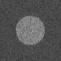
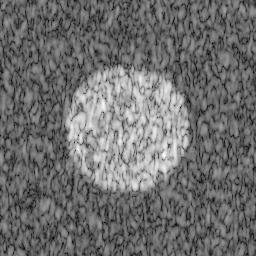
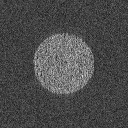
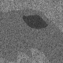
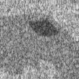
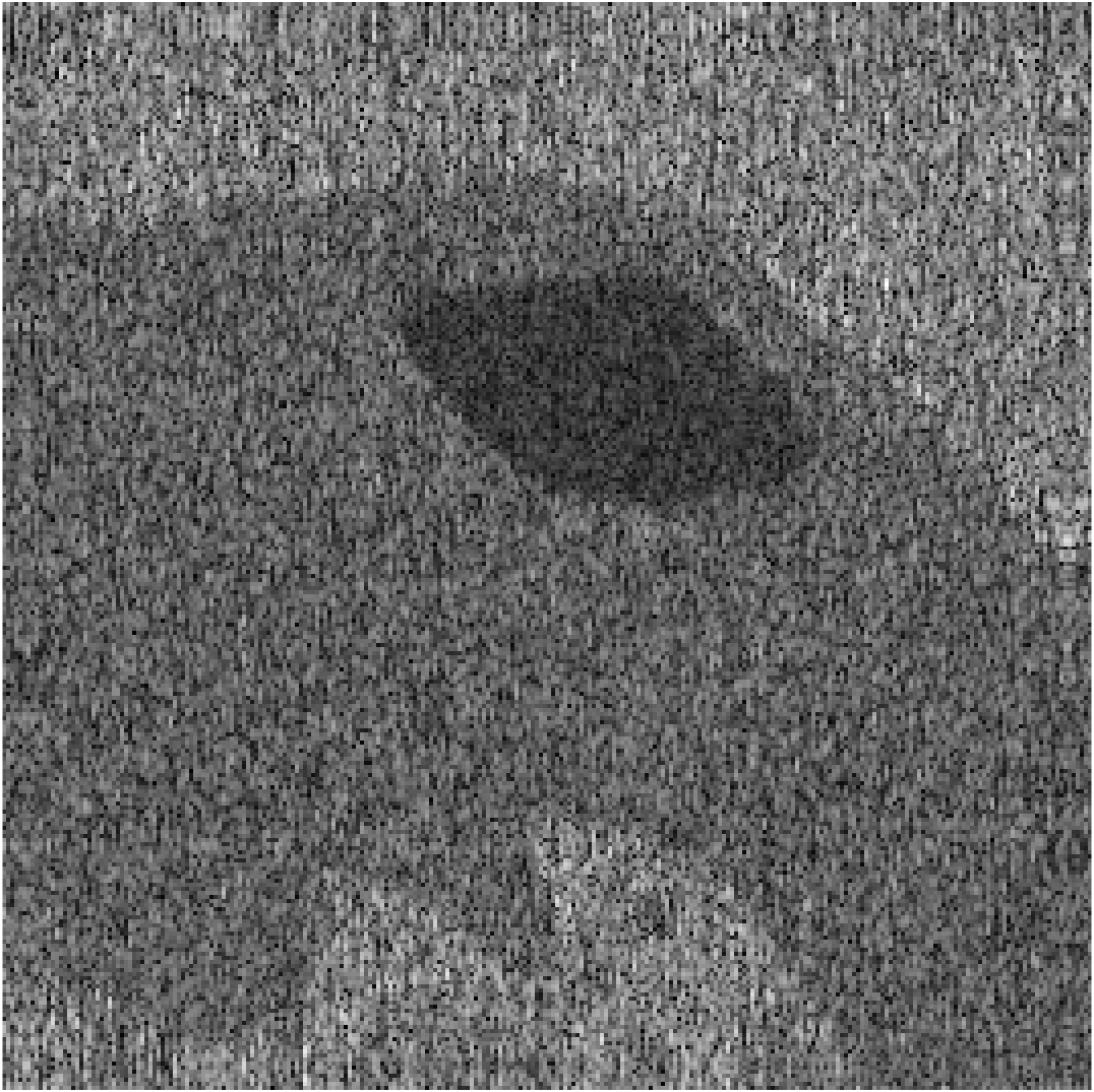
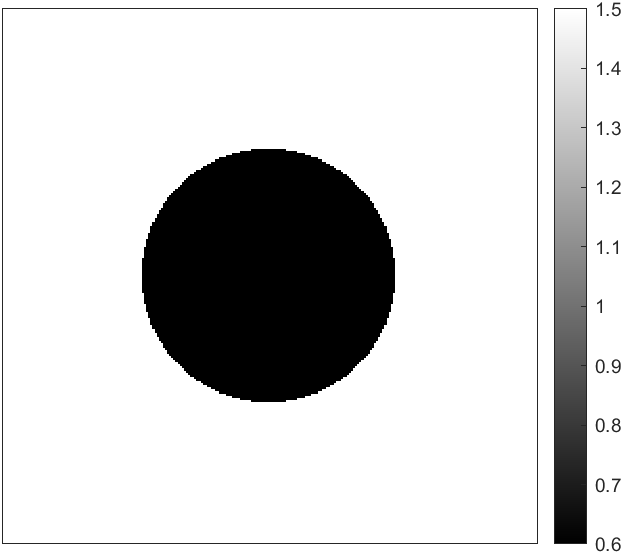
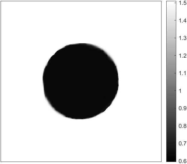
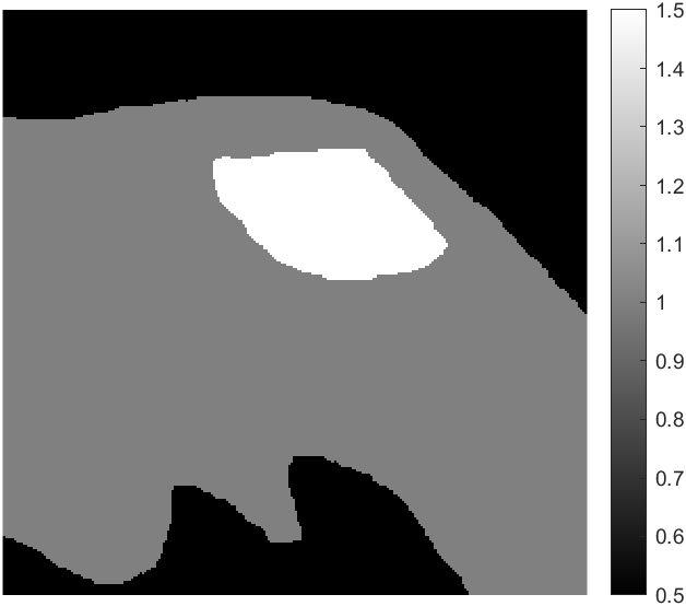
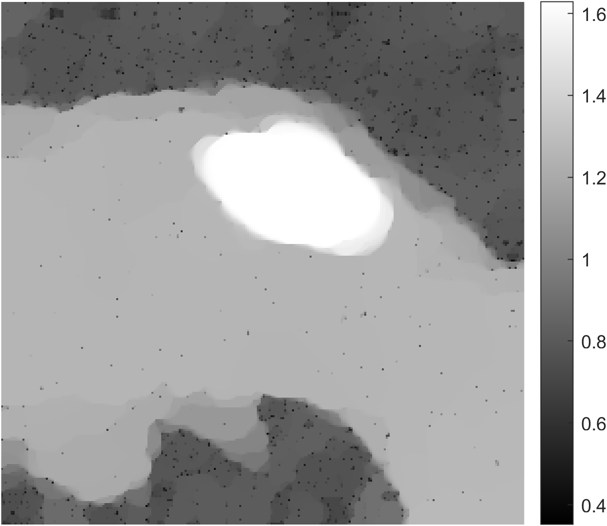
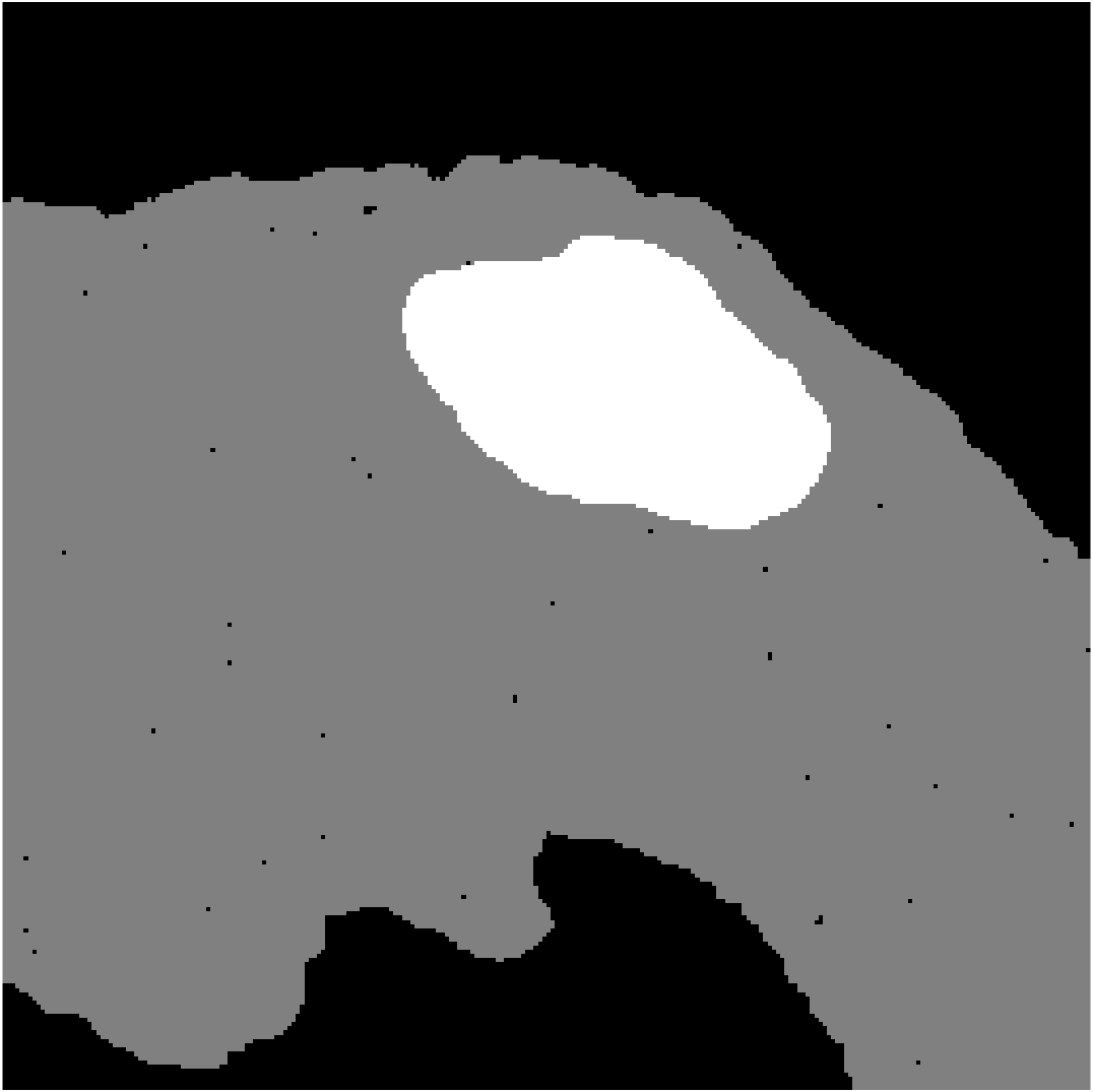
Figure 1 illustrates in the first and second line the B–mode image of the original , of the degraded , and of the reconstructed image on both examples. The B–mode image is the most common representation of an ultrasound image, displaying the acoustic impedance of a 2-dimensional cross section of the considered tissue. The reconstructed results in Figure 1 (right) show clearly reduced blur and sharper region contours. We then report in the third and fourth lines of Figure 1 the estimated shape parameter and the segmentation obtained via the aforementioned quantisation procedure, which confirms its good performance. We notice that our estimated values are consistent with the original ones and the fact that the results for Simu2 are slightly less accurate than the ones for Simu1 is in line with the results presented in [17, Table III] for P-ULA, HMC and PP-ULA, suggesting that the configuration of the parameters for Simu2 is quite challenging.
Table 1 proposes a quantitative comparison of our results against those of the methods considered in [17]: a combination of Wiener deconvolution and Otsu’s segmentation [45], a combination of LASSO deconvolution and SLaT segmentation [38], the adjusted Hamiltonian Monte Carlo (HMC) method [77], the Proximal Unadjusted Langevin algorithm (P-ULA) [78] and its preconditioned version (PP-ULA) [17] for joint deconvolution and segmentation. From this table we can conclude that the proposed variational method is able to compete with state-of-the-art Monte Carlo Markov Chain techniques in terms of both segmentation and deconvolution performance. For what concerns the computational time, the average time (over 10 runs of the algorithm) required by P-SASL-PAM to meet the stopping criteria and corresponds to seconds (approximately ) for Simu1 and seconds (approximately ) for Simu2. Simulations were run on Matlab 2021b on an Intel Xeon Gold 6230 CPU 2.10GHz. In Table 1 we report the computational times from for PULA, HMC and PP-ULA from [17, TABLE II], which were obtained on Matlab 2018b on an Intel Xeon CPU E5-1650 3.20GHz.
| Simu1 | Simu2 | |||||||
| METHOD | PSNR | SSIM | OA | TIME | PSNR | SSIM | OA | TIME |
| Wiener-Otsu | 37.1 | 0.57 | 99.5 | – | 35.4 | 0.63 | 96.0 | – |
| LASSO-SLaT | 39.2 | 0.60 | 99.6 | – | 37.8 | 0.70 | 98.3 | – |
| P-ULA | 38.9 | 0.45 | 98.7 | h min | 37.1 | 0.57 | 94.9 | h min |
| HMC | 40.0 | 0.62 | 99.7 | h min | 36.4 | 0.64 | 98.5 | h min |
| PP-ULA | 40.3 | 0.62 | 99.7 | min | 38.6 | 0.71 | 98.7 | min |
| OURS | 40.2 | 0.61 | 99.9 | min | 38.1 | 0.70 | 97.7 | min |
| ORIGINAL | DEGRADED | RECONSTRUCTED | |
|
Simu1 |
|
|
|
|
Simu2 |
|
|
|
| REFERENCE | ESTIMATED | QUANTISED | |
| Simu1 |
|
|

|
| Simu2 |
|
|
|
 |
 |
 |
 |
| (a) | (b) | (c) | (d) |
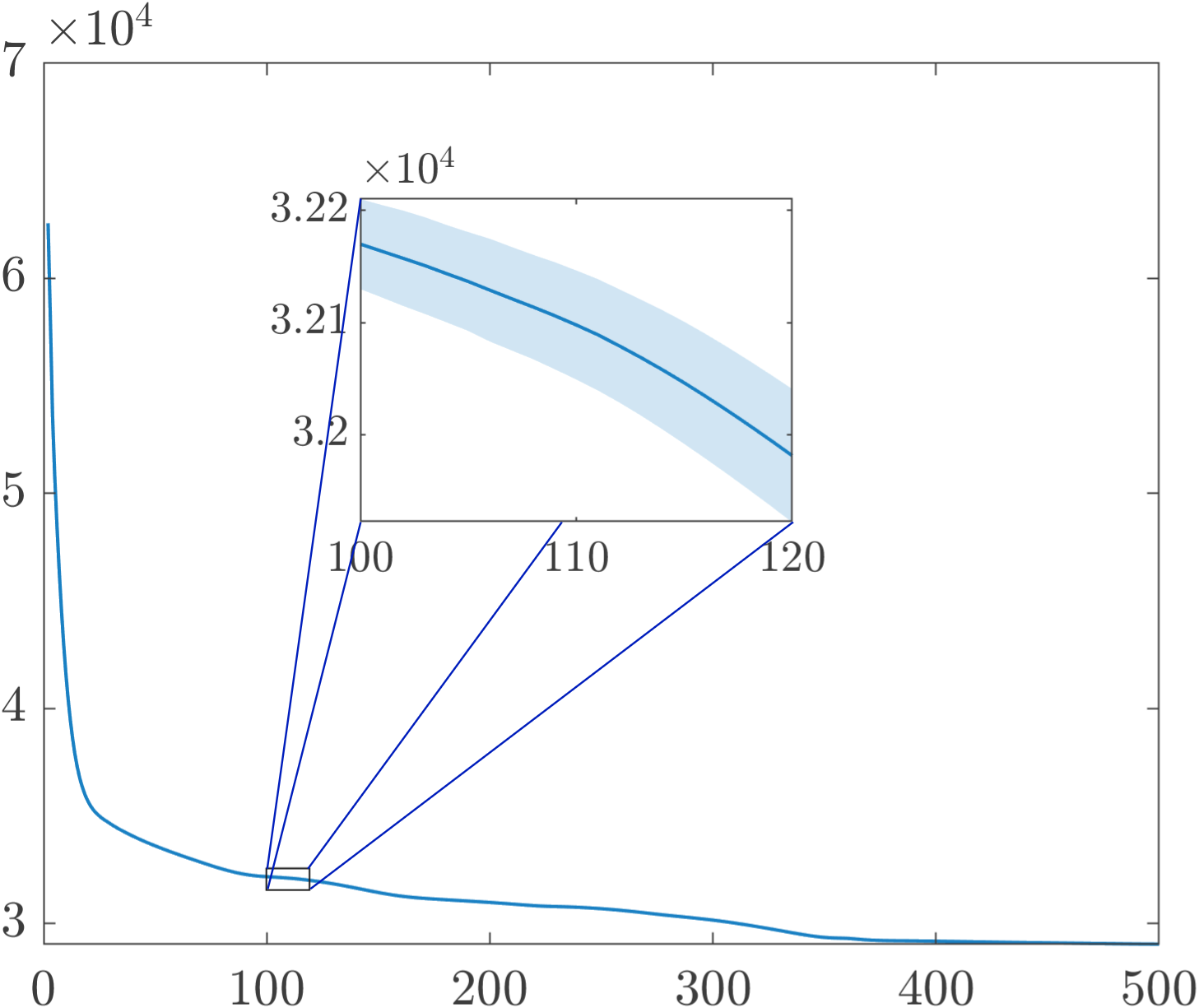
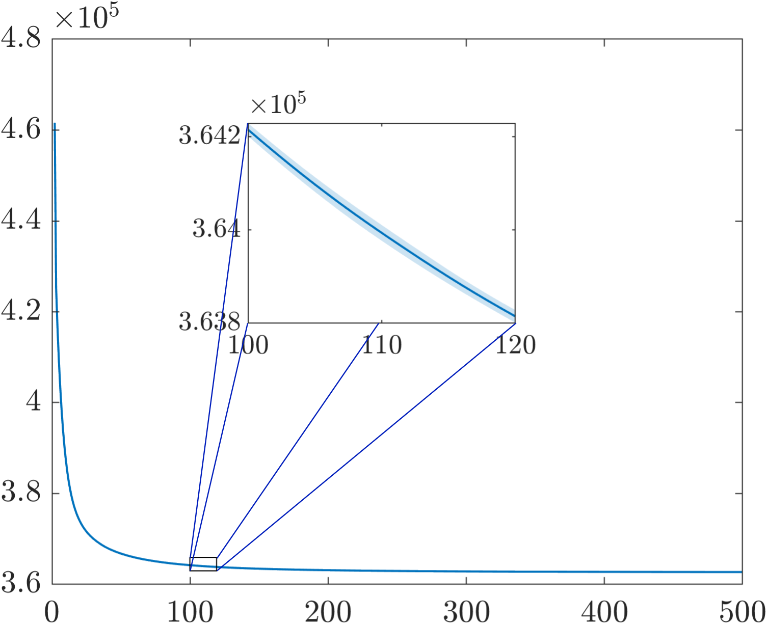
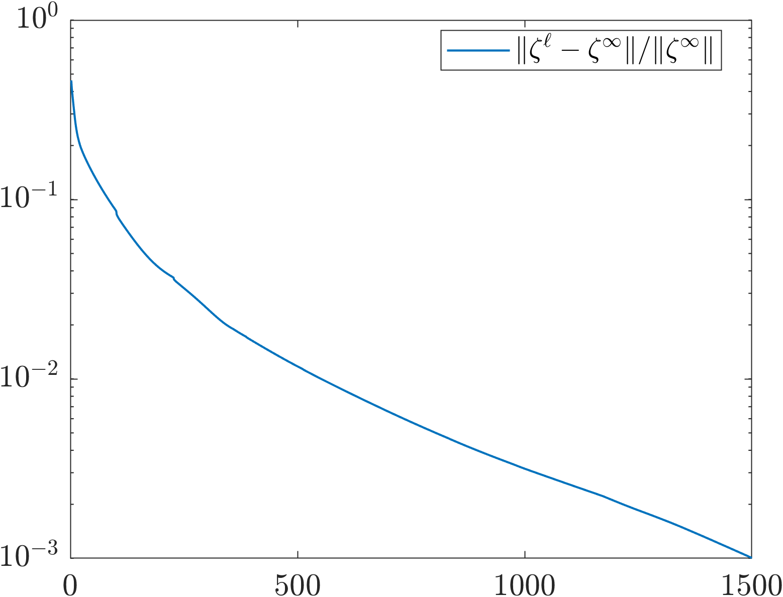
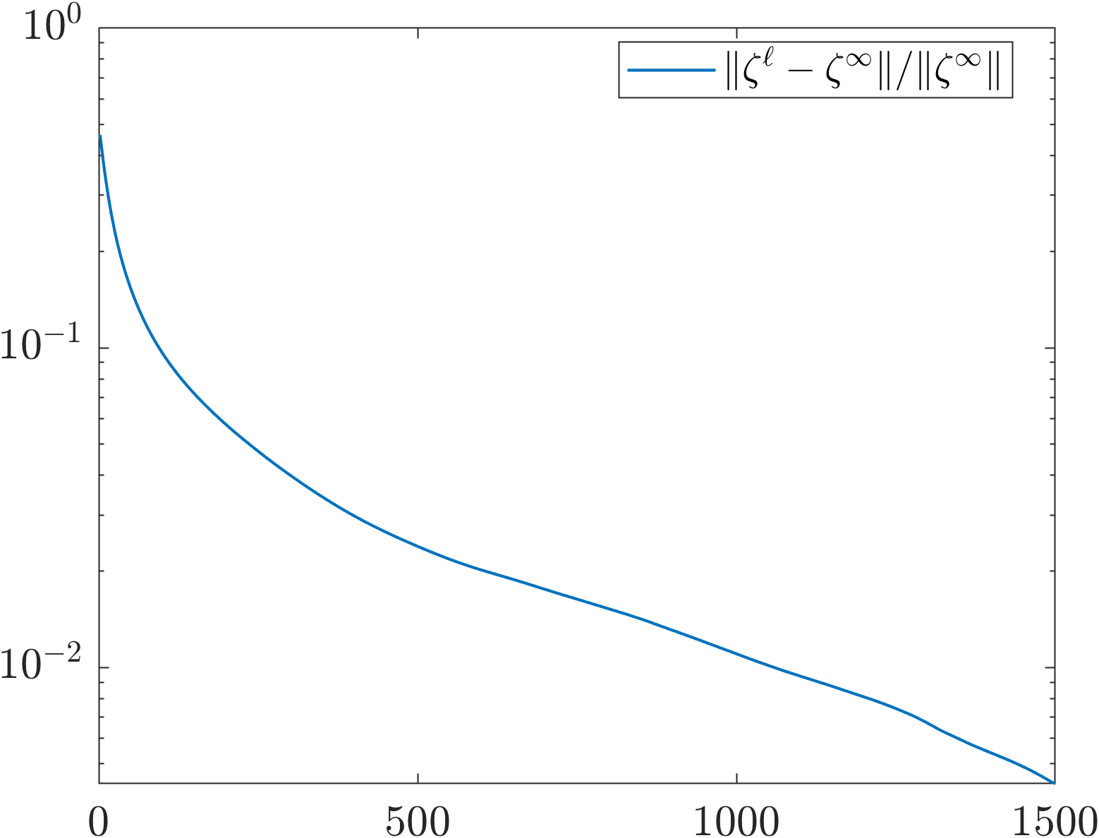
Eventually, Figure 2 (a)-(b) show the evolution of the mean value of the cost function for both Simu1 (a) and Simu2 (b) along 500 iterations for 10 different sampling of and , while Figure 2 (c)-(d)illustrate on a logarithmic scale the relative distance from the iterates to the solution for Simu1 (c) and Simu2 (d), showing the convergence of our algorithm.
Additional experiments can be found in Supplementary Material: SM1, showing that for standard wavelet-based image restoration problems the proposed regularisation outperforms other sparsity measures.
6 Conclusions
We investigated a novel approach for the joint reconstruction-feature extraction problem. The novelty in this work lies both in the problem formulation and in the resolution procedure. Firstly, we proposed a new variational model in which we introduced a flexible sparse regularisation term for the reconstruction task. Secondly, we designed an inexact version of a TITAN-based block alternating optimisation scheme, whose aim is to exploit the structure of the problem and the properties of the functions involved in it. We established convergence results for the proposed algorithm whose scope goes beyond the image processing problems considered in our work. We illustrated the validity of the approach on numerical examples in the case of a joint deconvolution-segmentation problem. We also included comparisons with state-of-the-art methods with respect to which our proposal registers a similar qualitative and quantitative performance. An attractive aspect of the proposed work is that the space variant parameters defining the flexible sparse regularisation do not need to be defined in advance, but are inherently estimated by the iterative optimisation procedure. For what concerns the tuning of the hyperparamters of the model, the design of an automatic strategy could be an interesting development of the work, for instance through supervised learning. \bmheadAcknowledgments This project has received funding from the European Union’s Horizon 2020 research and innovation programme under the Marie Skłodowska-Curie grant agreement No 861137. The authors thank Ségolène Martin for her careful reading of the initial version of this manuscript.
References
- \bibcommenthead
- Daubechies et al. [2004] Daubechies, I., Defrise, M., De Mol, C.: An iterative thresholding algorithm for linear inverse problems with a sparsity constrains. Communications on Pure and Applied Mathematics 57 (2004)
- Grasmair et al. [2008] Grasmair, M., Haltmeier, M., Scherzer, O.: Sparse regularization with lq penalty term. Inverse Problems 24, 055020 (2008)
- Lorenz [2008] Lorenz, D.: Convergence rates and source conditions for Tikhonov regularization with sparsity constraints. Journal of Inverse and Ill-posed Problems 16(5), 463–478 (2008)
- Ramlau and Resmerita [2010] Ramlau, R., Resmerita, E.: Convergence rates for regularization with sparsity constraints. Electronic transactions on numerical analysis ETNA 37, 87–104 (2010)
- Tibshirani [1996] Tibshirani, R.: Regression shrinkage and selection via the Lasso. Journal of the Royal Statistical Society: Series B (Methodological) 58, 267–288 (1996)
- Chartrand [2007] Chartrand, R.: Exact reconstruction of sparse signals via nonconvex minimization. IEEE Signal Processing Letters 14, 707–710 (2007)
- Grasmair [2009] Grasmair, M.: Well-posedness and convergence rates for sparse regularization with sublinear penalty term. Inverse Problems Imaging 3(3), 383–387 (2009)
- Zarzer [2009] Zarzer, C.: On Tikhonov regularization with non-convex sparsity constraints. Inverse Problems 25, 025006 (2009)
- Ghilli and Kunisch [2019] Ghilli, D., Kunisch, K.: On monotone and primal-dual active set schemes for -type problems, . Computational Optimization and Applications 72, 45–85 (2019)
- Hintermüller and Wu [2013] Hintermüller, M., Wu, T.: Nonconvex TVq-models in image restoration: analysis and a Trust-Region regularization-based superlinearly convergent solver. SIAM Journal on Imaging Sciences 6, 1385–1415 (2013)
- Lorenz and Resmerita [2016] Lorenz, D., Resmerita, E.: Flexible sparse regularization. Inverse Problems 33 (2016)
- Afonso and Sanches [2017] Afonso, M., Sanches, J.M.: Adaptive order non-convex lp-norm regularization in image restoration. Journal of Physics: Conference Series 904(1), 012016 (2017)
- Blomgren et al. [1997] Blomgren, P., Chan, T.F., Mulet, P., Wong, C.K.: Total variation image restoration: Numerical methods and extensions. IEEE International Conference on Image Processing (1997)
- Chen et al. [2006] Chen, Y., Levine, S., Rao, M.: Variable exponent, linear growth functionals in image restoration. SIAM Journal on Applied Mathematics 66, 1383–1406 (2006)
- Lanza et al. [2018] Lanza, A., Morigi, S., Pragliola, M., Sgallari, F.: Space-variant generalised Gaussian regularisation for image restoration. Computer Methods in Biomechanics and Biomedical Engineering: Imaging and Visualization 7, 1–14 (2018)
- Lazzaretti et al. [2022] Lazzaretti, M., Calatroni, L., Estatico, C.: Modular-proximal gradient algorithms in variable exponent lebesgue spaces. SIAM Journal on Scientific Computing 44(6), 3463–3489 (2022)
- Corbineau et al. [2019] Corbineau, M.-C., Kouamé, D., Chouzenoux, E., Tourneret, J.-Y., Pesquet, J.-C.: Preconditioned P-ULA for joint deconvolution-segmentation of ultrasound images. IEEE Signal Processing Letters 26(10), 1456–1460 (2019)
- Do and Vetterli [2002] Do, M.N., Vetterli, M.: Wavelet-based texture retrieval using generalized Gaussian density and Kullback-Leibler distance. IEEE Transactions on Image Processing 11(2), 146–158 (2002)
- Zhao et al. [2016] Zhao, N., Basarab, A., Kouamé, D., Tourneret, J.-Y.: Joint segmentation and deconvolution of ultrasound images using a hierarchical Bayesian model based on generalized Gaussian priors. IEEE Transactions on Image Processing 25(8), 3736–3750 (2016)
- Hildreth [1957] Hildreth, C.: A quadratic programming procedure. Naval Research Logistics Quarterly 4(1), 79–85 (1957)
- Tseng [2001] Tseng, P.: Convergence of a block coordinate descent method for nondifferentiable minimization. Journal of Optimization Theory and Applications 109, 475–494 (2001)
- Combettes and Pesquet [2011] Combettes, P.L., Pesquet, J.-C.: Proximal splitting methods in signal processing, pp. 185–212. Springer, New York, NY (2011)
- Combettes and Pesquet [2021] Combettes, P.L., Pesquet, J.-C.: Fixed point strategies in data science. IEEE Transactions on Signal Processing 69, 3878–3905 (2021)
- Attouch et al. [2010] Attouch, H., Bolte, J., Redont, P., Soubeyran, A.: Proximal alternating minimization and projection methods for nonconvex problems: an approach based on the Kurdyka-Łojasiewicz inequality. Mathematics of Operations Research 35(2), 438–457 (2010)
- Bolte et al. [2014] Bolte, J., Sabach, S., Teboulle, M.: Proximal alternating linearized minimization for nonconvex and nonsmooth problems. Mathematical Programming 146(1-2), 459–494 (2014)
- Pock and Sabach [2016] Pock, T., Sabach, S.: Inertial proximal alternating linearized minimization (iPALM) for nonconvex and nonsmooth problems. SIAM Journal on Imaging Sciences 9(4), 1756–1787 (2016)
- Hertrich and Steidl [2022] Hertrich, J., Steidl, G.: Inertial stochastic palm and applications in machine learning. Sampling Theory, Signal Processing, and Data Analysis 20(1), 4 (2022)
- Foare et al. [2020] Foare, M., Pustelnik, N., Condat, L.: Semi-Linearized proximal alternating minimization for a discrete Mumford–Shah model. IEEE Transactions on Image Processing 29, 2176–2189 (2020)
- Nikolova and Tan [2017] Nikolova, M., Tan, P.: Alternating proximal gradient descent for nonconvex regularised problems with multiconvex coupling terms (2017). https://hal.archives-ouvertes.fr/hal-01492846
- Tan et al. [2019] Tan, P., Pierre, F., Nikolova, M.: Inertial alternating generalized forward–backward splitting for image colorization. Journal of Mathematical Imaging and Vision 61, 672–690 (2019)
- Censor and Lent [1987] Censor, Y., Lent, A.: Optimization of “log x" entropy over linear equality constraints. Siam Journal on Control and Optimization 25, 921–933 (1987)
- Chouzenoux et al. [2016] Chouzenoux, E., Pesquet, J.-C., Repetti, A.: A block coordinate variable metric forward–backward algorithm. Journal of Global Optimization, 1–29 (2016)
- Bonetti et al. [2018] Bonetti, S., Prato, M., Rebegoldi, S.: A block coordinate variable metric linesearch based proximal gradient method. Computational Optimization and Applications (2018)
- Repetti and Wiaux [2021] Repetti, A., Wiaux, Y.: Variable metric forward-backward algorithm for composite minimization problems. SIAM Journal on Optimization 31(2), 1215–1241 (2021)
- Bonettini et al. [2019] Bonettini, S., Porta, F., Prato, M., Rebegoldi, S., Ruggiero, V., Zanni, L.: Recent Advances in Variable Metric First-Order Methods, pp. 1–31. Springer, Cham (2019)
- Hien et al. [2020] Hien, L.T.K., Phan, D.N., Gillis, N.: An inertial block majorization minimization framework for nonsmooth nonconvex optimization. J. Mach. Learn. Res. 24, 18–11841 (2020)
- Attouch et al. [2011] Attouch, H., Bolte, J., Svaiter, B.F.: Convergence of descent methods for semi-algebraic and tame problems: proximal algorithms, forward-backward splitting, and regularized Gauss-Seidel methods. Mathematical Programming, Series A 137(1), 91–124 (2011)
- Cai et al. [2017] Cai, X., Chan, R., Nikolova, M., Zeng, T.: A three-stage approach for segmenting degraded color images: Smoothing, Lifting and Thresholding (SLaT). Journal of Scientific Computing 72, 1313–1332 (2017)
- Cai et al. [2019] Cai, X., Chan, R., Schönlieb, C.-B., Steidl, G., Zeng, T.: Linkage between piecewise constant Mumford–Shah model and Rudin–Osher–Fatemi model and its virtue in image segmentation. SIAM Journal on Scientific Computing 41(6), 1310–1340 (2019)
- Cai et al. [2013] Cai, X., Chan, R., Zeng, T.: A two-stage image segmentation method using a convex variant of the Mumford–Shah model and thresholding. SIAM Journal on Imaging Sciences 6(1), 368–390 (2013)
- Chambolle et al. [2012] Chambolle, A., Cremers, D., Pock, T.: A convex approach to minimal partitions. SIAM Journal on Imaging Sciences 5, 1113–1158 (2012)
- Chan et al. [2014] Chan, R., Yang, H., Zeng, T.: A two-stage image segmentation method for blurry images with Poisson or multiplicative Gamma noise. SIAM Journal on Imaging Sciences 7(1), 98–127 (2014)
- Pascal et al. [2021] Pascal, B., Vaiter, S., Pustelnik, N., Abry, P.: Automated data-driven selection of the hyperparameters for total-variation based texture segmentation. Journal of Mathematical Imaging and Vision 63, 923–952 (2021)
- Mumford and Shah [1989] Mumford, D., Shah, J.: Optimal approximations by piecewise smooth functions and associated variational problems. Communications on Pure and Applied Mathematics 42, 577–685 (1989)
- Otsu [1979] Otsu, N.: A threshold selection method from gray-level histograms. IEEE Transactions on Systems, Man, and Cybernetics 9(1), 62–66 (1979)
- Rockafellar et al. [2009] Rockafellar, R.T., Wets, M., Wets, R.J.B.: Variational Analysis. Grundlehren der mathematischen Wissenschaften. Springer, Heidelberg (2009)
- Kurdyka [1998] Kurdyka, K.: On gradients of functions definable in o-minimal structures. Annales de l’Institut Fourier 48(3), 769–783 (1998)
- Łojasiewicz [1963] Łojasiewicz, S.: Une propriété topologique des sous-ensembles analytiques réels. Equ. Derivees partielles, Paris 1962, Colloques internat. Centre nat. Rech. sci. 117, 87-89 (1963). (1963)
- Łojasiewicz [1993] Łojasiewicz, S.: Sur la géométrie semi- et sous- analytique. Annales de l’Institut Fourier 43(5), 1575–1595 (1993)
- Chouzenoux et al. [2014] Chouzenoux, E., Pesquet, J.-C., Repetti, A.: Variable metric Forward-Backward algorithm for minimizing the sum of a differentiable function and a convex function. Journal of Optimization Theory and Applications 162, 107–132 (2014)
- Bertsekas [1999] Bertsekas, D.P.: Nonlinear Programming, 2nd edn. Athena Scientific, Nashua (1999)
- Erdogan and Fessler [1999] Erdogan, H., Fessler, J.A.: Monotonic algorithms for transmission tomography. IEEE Transactions on Medical Imaging 18(9), 801–814 (1999)
- Hunter and Lange [2004] Hunter, D., Lange, K.: A Tutorial on MM Algorithms. The American Statistician 58, 30–37 (2004)
- Salzo [2017] Salzo, S.: The variable metric forward-backward splitting algorithm under mild differentiability assumptions. SIAM Journal on Optimization 27(4), 2153–2181 (2017)
- Malitsky and Mishchenko [2020] Malitsky, Y., Mishchenko, K.: Adaptive gradient descent without descent. In: III, H.D., Singh, A. (eds.) Proceedings of the 37th International Conference on Machine Learning. Proceedings of Machine Learning Research, vol. 119, pp. 6702–6712 (2020)
- Latafat et al. [2023] Latafat, P., Themelis, A., Stella, L., Patrinos, P.: Adaptive proximal algorithms for convex optimization under local Lipschitz continuity of the gradient (2023)
- Charbonnier et al. [1997] Charbonnier, P., Blanc-Féraud, L., Aubert, G., Barlaud, M.: Deterministic edge-preserving regularization in computed imaging. IEEE Transactions on Image Processing 6 2, 298–311 (1997)
- Van Den Dries [1998] Van Den Dries, L.: Tame Topology and O-minimal Structures. London Mathematical Society Lecture Note Series. Cambridge University Press, Cambridge (1998)
- Bolte et al. [2007] Bolte, J., Daniilidis, A., Lewis, A., Shiota, M.: Clarke subgradients of stratifiable functions. SIAM Journal on Optimization 18(2), 556–572 (2007)
- Gabrielov [1996] Gabrielov, A.: Complements of subanalytic sets and existential formulas for analytic functions. Inventiones mathematicae 125, 1–12 (1996)
- Wilkie [1996] Wilkie, A.: Model completeness results for expansions of the ordered field of real numbers by restricted Pfaffian functions and the exponential function. Journal of the American Mathematical Society 9, 1051–1094 (1996)
- Van Den Dries et al. [1997] Van Den Dries, L., Macintyre, A., Marker, D.: Logarithmic-exponential power series. Journal of the London Mathematical Society 56(3), 417–434 (1997)
- Van Den Dries and Speissegger [2000] Van Den Dries, L., Speissegger, P.: The field of reals with multisummable series and the exponential function. Proceedings of The London Mathematical Society 81, 513–565 (2000)
- Tougeron [1994] Tougeron, J.: Sur les ensembles semi-analytiques avec conditions gevrey au bord. Annales Scientifiques De L Ecole Normale Superieure 27, 173–208 (1994)
- Artin [2015] Artin, E.: The Gamma Function. Courier Dover Publications, New York (2015)
- Wrench [1968] Wrench, J.W.: Concerning two series for the Gamma function. Mathematics of Computation 22(103), 617–626 (1968)
- Andrews et al. [1999] Andrews, G.E., Askey, R., Roy, R.: Special Functions. Encyclopedia of Mathematics and its Applications. Cambridge University Press, Cambridge (1999)
- Repetti and Wiaux [2021] Repetti, A., Wiaux, Y.: Variable metric forward-backward algorithm for composite minimization problems. SIAM Journal on Optimization 31(2), 1215–1241 (2021)
- Schifano et al. [2010] Schifano, E.D., Strawderman, R.L., Wells, M.T.: Majorization-Minimization algorithms for nonsmoothly penalized objective functions. Electronic Journal of Statistics 4(none), 1258–1299 (2010)
- Combettes et al. [2011] Combettes, P.L., Dũng, Bằng Công Vũ: Proximity for sums of composite functions. Journal of Mathematical Analysis and Applications 380(2), 680–688 (2011)
- Condat [2013] Condat, L.: A Primal–Dual splitting method for convex optimization involving lipschitzian, proximable and linear composite terms. Journal of Optimization Theory and Applications 158 (2013)
- Komodakis and Pesquet [2015] Komodakis, N., Pesquet, J.-C.: Playing with duality: An overview of recent primal-dual approaches for solving large-scale optimization problems. IEEE Signal Processing Magazine 32(6), 31–54 (2015)
- Vũ [2013] Vũ, B.C.: A splitting algorithm for dual monotone inclusions involving cocoercive operators. Advances in Computational Mathematics 38, 667–681 (2013)
- Corless et al. [1996] Corless, R., Gonnet, G., Hare, D., Jeffrey, D., Knuth, D.: On the Lambert W function. Advances in Computational Mathematics 5, 329–359 (1996)
- Jensen [2004] Jensen, J.A.: Simulation of advanced ultrasound systems using field ii. In: 2004 2nd IEEE International Symposium on Biomedical Imaging: Nano to Macro, pp. 636–6391 (2004)
- Wang et al. [2004] Wang, Z., Bovik, A.C., Sheikh, H.R., Simoncelli, E.P.: Image quality assessment: from error visibility to structural similarity. IEEE Transactions on Image Processing 13(4), 600–612 (2004)
- Robert et al. [2018] Robert, C., Elvira, V., Tawn, N., Wu, C.: Accelerating MCMC algorithms. Wiley Interdisciplinary Reviews: Computational Statistics 10 (2018)
- Pereyra [2013] Pereyra, M.: Proximal Markov chain Monte Carlo algorithms. Statistics and Computing 26 (2013)