CALET Collaboration
Observation of Spectral Structures in the Flux of Cosmic-Ray Protons
from 50 GeV to 60 TeV with the Calorimetric Electron Telescope on International Space Station
Abstract
A precise measurement of the cosmic-ray proton spectrum with the Calorimetric Electron Telescope (CALET) is presented in the energy interval from 50 GeV to 60 TeV and the observation of a softening of the spectrum above 10 TeV is reported. The analysis is based on the data collected during 6.2 years of smooth operations aboard the International Space Station (ISS) and covers a broader energy range with respect to the previous proton flux measurement by CALET, with an increase of the available statistics by a factor of 2.2. Above a few hundred GeV we confirm our previous observation of a progressive spectral hardening with a higher significance (more than 20 sigma). In the multi-TeV region we observe a second spectral feature with a softening around 10 TeV and a spectral index change from to consistently, within the errors, with the shape of the spectrum reported by DAMPE. We apply a simultaneous fit of the proton differential spectrum which well reproduces the gradual change of the spectral index encompassing the lower energy power-law regime and the two spectral features observed at higher energies.
pacs:
96.50.sb,95.35.+d,95.85.Ry,98.70.Sa,29.40.VjRecent direct measurements of cosmic rays have shown the presence of unexpected spectral structures significantly departing from a simple-power-law dependence.
The presence of a spectral hardening has been established for several nuclear species Panov et al. (2007); Ahn et al. (2009, 2010); Yoon et al. (2011); Adriani et al. (2011); Aguilar et al. (2015a, b); Yoon et al. (2017); Aguilar et al. (2017, 2018a, 2018b); Adriani et al. (2019a); Adriani (2019) around a few hundred GeV/
and high statistics measurements have shown that the rigidity dependence of primary and secondary cosmic nuclei is different AMS02_NeMgSi .
This rich phenomenology has been addressed by several theoretical models
in the quest for a consistent picture of cosmic-ray acceleration (eventually including new sources) Ellison et al. (1997); Malkov et al. (2012); Erlykin and Wolfendale (2012); Drury (2011); Ohira et al. (2016); Biermann et al. (2010); Ptuskin et al. (2013); Zatsepin and Sokolskaya (2006); Vladimirov et al. (2012); Kawanaka and Yanagita (2018), propagation (or reacceleration) in the Galaxy Blasi et al. (2012); Aloisio and Blasi (2013); Thoudam and Hörandel (2014); Tomassetti (2012, 2015); Giacinti et al. (2018); Evoli et al. (2018) and the possible presence of one or more local sources Thoudam and Hörandel (2012); Bernard et al. (2013).
More recent theoretical contributions were presented at the International Cosmic Ray 2021 Conference Lipari (2021); Recchia (2021); Caprioli Haggerty, Blasi ; CristofariBlasi, Amato ; Morlino (2021). The hypothesis of a possible charge-dependent cutoff in the nuclei spectra can be directly tested with long duration measurements in space, provided they achieve a sufficient exposure, adequate energy resolution, and the capability to identify individual elements.
New data from space-borne calorimetric instruments have recently become available, expanding the energy frontier of proton measurements by more than 1 order of magnitude. Following our previous observation up to 10 TeV of a spectral hardening of the proton spectrum
around a few hundred GeV,
a new feature emerged above 10 TeV whereby the spectral index was found to gradually change and a softening of the spectrum was clearly observed, as also reported by DAMPE DAMPE_proton and CALET K. Kobayashi and P.S. Marrocchesi (2021) and previously by NUCLEON Atkin et al. (2018)
and CREAM-III CREAM3_proton .
For proton and helium, it is important to determine the detailed rigidity dependence of the spectral index through the whole spectrum, studying the onset of the spectral hardening and of the softening regime at higher energy, respectively.
In order to achieve a consistent picture, systematic errors should be kept under control and a critical comparison of the observations from different experiments should be fostered.
The Calorimetric Electron Telescope (CALET)
Marrocchesi (2021); Asaoka et al. (2018), in operation on the International Space Station since 2015, is
a calorimetric instrument optimized for the measurement of the all-electron spectrum Adriani et al. (2017a, 2018).
It has enough depth, dynamic range, and energy resolution to
measure protons, helium P. Brogi and K.Kobayashi (2021), and heavier cosmic-ray nuclei
(up to iron and above) Adriani (2019); ICRC2021_carbon ; Y.Akaike and Y.Akaike (2021); Adriani et al. (2018); F.Stolzi, C.Checchia and C.Checchia (2021); Adriani et al. (2018); ICRC2021_Zober at energies reaching the PeV scale.
In this Letter, we present a direct measurement of the cosmic-ray proton differential spectrum in kinetic energy from 50 GeV to 60 TeV with CALET.
Designed to achieve a full containment of TeV electromagnetic showers and a large
electron-proton discrimination capability (105), it is longitudinally segmented into a fine grained imaging calorimeter (IMC) followed by a total absorption calorimeter (TASC). The TASC is a 27 (radiation length) thick homogeneous calorimeter with 12 alternate orthogonal layers of lead-tungstate logs.
The IMC is a sampling calorimeter segmented into 16 layers of individually read-out scintillating fibers (with 1 mm2 square cross section) and interspaced with thin tungsten absorbers. Alternate planes of fibers are arranged along orthogonal directions.
It can image the early shower profile in the first 3 and provide tracking information by reconstructing the incident direction of cosmic rays with good angular resolution (0.1∘ for electrons and better than 0.5∘ for hadrons) Torii (2019).
The overall thickness of CALET at normal incidence is 30 and 1.3 (proton interaction lengths).
The charge identification of individual nuclear species is performed by a two-layered hodoscope of plastic scintillators (CHD), positioned at the top of the apparatus, providing a measurement of the charge of the incident particle over a wide dynamic range ( to ) with sufficient charge resolution to resolve individual elements Mar2011 and complemented by a redundant charge determination via multiple measurements in the IMC.
The overall CHD charge resolution (in units)
increases linearly, as a function of the atomic number, from 0.1 for protons to 0.3 for iron. For the IMC,
multiple sampling in the IMC achieves an excellent performance as shown in
Ref. Pier-ICRC19 where the charge resolution is plotted as a function of the atomic number .
The interaction point (IP) is first reconstructed Brogi-ICRC15 , and only the ionization clusters from the layers upstream of the IP are used to infer a charge value from the truncated mean of the valid samples.
The geometrical factor of CALET is 0.1 m2sr, and the total weight is 613 kg. The instrument is described in more detail elsewhere Asaoka et al. (2017).
Flight data collected for 2272 days from October 13, 2015, to December 31, 2021, were analyzed.
The total observation live time with the high-energy (HE) shower trigger Asaoka et al. (2018)
is 1925 days. A low-energy (LE) shower trigger,
operated at high geomagnetic latitudes Asaoka et al. (2018), was also used for the analysis of the
low-energy region. As we have sufficient statistics for protons below 100 GeV,
we used the data presented in Ref. Adriani et al. (2019a).
A Monte Carlo (MC) simulation, based on the EPICS simulation package Kasahara (1995); EPI , was developed to reproduce the detailed detector configuration and physics processes, as well as detector signals. In order to assess the uncertainties due to the modeling of hadronic interactions, a series of beam tests were carried out at the CERN-SPS with proton beams of 30, 100, and 400 GeV. However, no beam test calibrations are possible beyond this limit with the available accelerated beams. Therefore simulations with FLUKA Böhlen (2014); Ferrari et al. (2005); FLU and GEANT4 Agostinelli et al. (2003); Gea were compared with EPICS, and the differences were properly accounted for in the systematic uncertainties. Trigger efficiency and energy response derived from MC simulations were extensively studied Adriani et al. (2019a).
As described in our previous publication Adriani et al. (2019a), the track of the primary cosmic-ray particle was reconstructed from the hit pattern of the IMC fibers by means of a Kalman filter tracking package Maestro et al. (2017) developed for CALET. The shower energy is calculated as the sum of the TASC energy deposits. The total observed energy () is calibrated using penetrating particles, and a seamless stitching of adjacent gain ranges is performed on orbit. This procedure was complemented by the confirmation of the linearity of the system over the whole range by means of ground measurements using a UV pulsed laser, as described in Ref. Asaoka et al. (2017). Temporal variations during the long-term observation period were also corrected for, using penetrating particles to monitor the gain of each sensor Adriani et al. (2017a).
In order to minimize the background contamination, the following criteria were applied to well-reconstructed and well-contained proton-events: (1) off-line trigger confirmation, (2) geometrical acceptance condition (requires acceptance type as defined in Ref. Adriani et al. (2018)), (3) reliability of the reconstructed track while retaining a high efficiency, (4) electron rejection, (5) rejection of off-acceptance events, (6) consistency of the track impact point in the TASC with the calorimetric energy deposits, (7) requirements on the shower development in the IMC, and (8) identification of the particle as a proton by using both CHD and IMC charge measurements.
Criterion (1) applies more stringent conditions with respect to the onboard trigger removing effects caused by positional and temporal variations of the detector gain. In the energy range GeV, the HE trigger should be asserted and the energy deposit sum of the IMC 7th and 8th layers is required to exceed 50 minimum ionizing particles (MIPs) in either the or view. Furthermore, the energy deposit of the first TASC layer (TASC-X1) should be larger than 100 MIPs. In the energy range GeV, the LE trigger should be asserted, the energy deposit sum of the IMC layers 7 and 8 should be greater than 5 MIPs in either the or view and the energy deposit of TASC-X1 should be larger than 10 MIPs. Criterion (3) requires the reliability of track fitting (details on track quality cuts can be found in the Supplemental Material of Ref. Adriani et al. (2019a)).
In order to reject electron events, a “Molière concentration” along the track is calculated by summing up all energy deposits observed inside one Molière radius for tungsten (9 fibers, i.e., 9 mm) around the IMC fiber best matched with the track. By requiring the ratio of the energy deposit within 9 mm to the total energy deposit sum in the IMC to be less than 0.7 [criterion (4)], most of the electrons are rejected while retaining an efficiency above 92% for protons.
In order to minimize the fraction of misidentified events, two topological cuts are applied using the TASC energy-deposit information only and irrespective of IMC tracking [criterion (5)]. These cuts remove poorly reconstructed events where one of the secondary tracks is identified as the primary track (refer to the Supplemental Material of Ref. Adriani et al. (2019a)).
Criterion (6) removes additional misreconstructed events by applying a consistency cut between the track impact point and the center of gravity of the energy deposits in the first and second (TASC-Y1) layers of the TASC.
In order to select well-contained events, energy dependent thresholds are set to achieve a 95% constant efficiency for events that interacted in the IMC below the fourth layer [criterion (7)]. After applying criteria (1) – (7), charge, energy, and trigger efficiency are determined for the selected sample (hereafter denoted as “target” events).
Backscattered particles from the calorimeter can affect both the trigger and the charge determination. In fact, primary particles below the trigger thresholds might be triggered anyway because of backscattered particles hitting the TASC-X1 and IMC bottom layers. Moreover a significant amount of backscatter may potentially induce a fake charge identification by increasing the number of hits with a significant energy deposit in IMC and CHD [criterion (8)].
The charge is calculated as , where is the CHD or IMC response (in MIP units) and and are energy dependent charge correction coefficients (mainly accounting for backscattering effects increasing with energy) applied separately to flight data, EPICS, FLUKA, and GEANT4 to optimize the determination of the charge peaks of proton and helium at and 2, respectively Adriani et al. (2019a).
A charge selection of proton candidates is performed by applying simultaneous window cuts on CHD and IMC reconstructed charges. Energy dependent criteria are defined for “target” events to maintain the same efficiency for the CHD and IMC. In the higher energy region, the identification using IMC is useful to reject helium events. Figure 1 shows examples of the distribution using IMC.
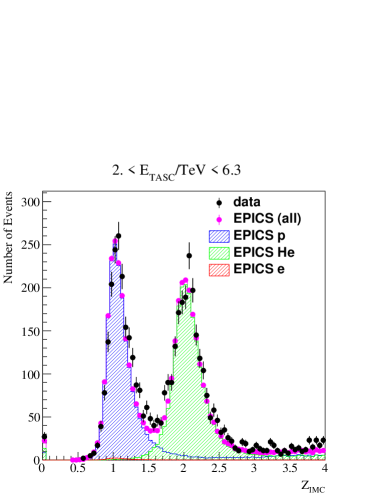
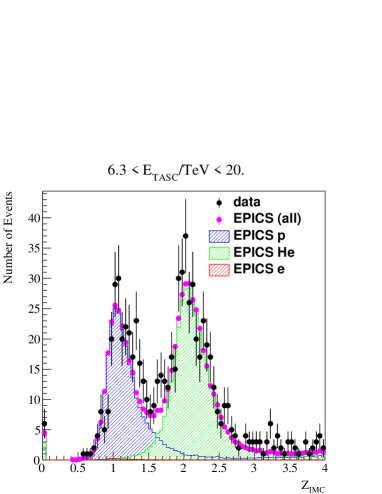
Further details on the selection criteria can be found in the Supplemental Material CAL and in Ref. Adriani et al. (2019a).
Background contamination is estimated using MC simulations of protons,
helium, and electrons.
Below TeV (TASC energy deposits sum), the dominant background comes from off-acceptance protons.
The contamination is estimated below a few percent.
At higher energies, helium is the main background source, and the contamination gradually increases with the observed energy reaching a maximum of 20% as shown in Fig. S2 of the Supplemental Material CAL .
A background contamination correction, based on the charge distribution, is applied
before application of the energy unfolding.
The calorimetric energy resolution for protons is around 30%–40% with an observed energy fraction close to 35%. Therefore, energy unfolding is required to correct for bin-to-bin migration effects. We follow a Bayesian approach, as implemented in the RooUnfold package Adye (2011); D’Agostini (1995) in ROOT Brun and Rademakers (1997), whereby the response matrix is derived from the MC simulations. The unfolded energy spectrum is presented and compared with the distribution in Fig. S3 of Supplemental Material CAL . Convergence is usually reached within two iterations, given the relatively accurate prior distribution obtained from the previous observations, i.e., by AMS-02 Aguilar et al. (2015a) and CREAM-III Yoon et al. (2017).
The proton spectrum is obtained by correcting the effective geometrical acceptance with the unfolded energy distribution as follows:
where denotes the energy bin width, the
unfolding procedure operator based on the Bayes theorem, the
bin counts of the unfolded distribution, those
of the observed energy distribution (including background), the bin counts
of background events in the observed energy distribution,
the effective acceptance including all selection efficiencies, and the live time.
At the lowest energies, the HE-trigger efficiency drops significantly, and in this region LE-trigger events are
used instead. The event selection criteria for the HE and LE analyses are identical.
While the overall difference between the two selections is relatively small, the difference in the
low-energy region is sizeable while, in the energy region above 200 GeV, LE- and HE-trigger data are consistent.
Therefore we use LE-trigger data for GeV and HE-trigger data above.
The fluxes obtained with LE and HE triggers are presented within the respective energy regions in Fig. S4 of Supplemental Material CAL .
The systematic uncertainties include energy independent and dependent contributions.
The former is estimated around 4.1% in total, from
the uncertainties on the live time (3.4%), radiation environment
(1.8%), and long-term stability (1.4%).
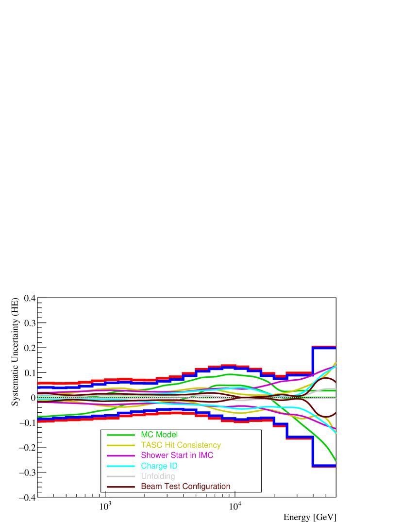
The energy dependent component is estimated to be less than 10% for TeV.
We take into account the uncertainties on MC model dependence,
IMC track consistency with the TASC energy deposits, shower start in the IMC, charge identification,
energy unfolding, and beam test configuration. For TeV the uncertainties
on MC model dependence and charge identification become dominant.
In the interval TeV the uncertainty is below 20% while reaching
a maximum 30% in the last bin.
Figure 2 shows the systematic uncertainty in the HE
sample as a function of energy.
Our extended measurement of the proton spectrum from 50 GeV to 60 TeV
is shown in Fig. 3. The CALET flux is compared with AMS-02 Aguilar et al. (2015a), DAMPE DAMPE_proton , and CREAM-III CREAM3_proton .
Our spectrum is in good agreement with the rigidity spectra measured by magnetic spectrometers in the sub-TeV region, and it is also consistent, within the errors, with the measurements carried out with calorimetric instruments at higher energies.
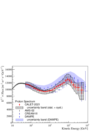
Our data confirm the presence of a spectral hardening at a few hundred GeV as reported in our previous proton Letter Adriani et al. (2019a) with a higher significance of more than 20 sigma (statistical error). We also observe a spectral softening around 10 TeV.
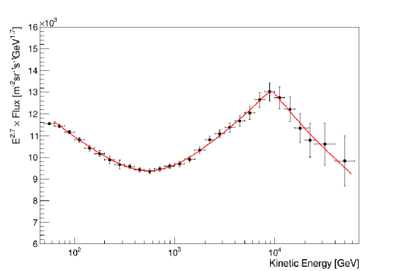
We fit the proton spectrum in the energy region from 80 GeV to 60 TeV with a double broken power law (DBPL) function defined as follows:
| (1) |
with:
| (2) |
where is the proton flux, is a normalization factor, the spectral index, is a characteristic energy of the region where a gradual spectral hardening is observed, the spectral variation due to the spectral hardening, is a characteristic energy of the transition to the region of spectral softening, and is the spectral index variation observed above . Two independent smoothness parameters and are introduced in the energy intervals where spectral hardening and softening occur, respectively.
CALET data (black filled circles) and associated statistical errors are shown in Fig. 4 where the red line shows the best fitted function with parameters
, , , GeV, , TeV, and 30 with a large error.
The is 4.4 with 20 degrees of freedom.
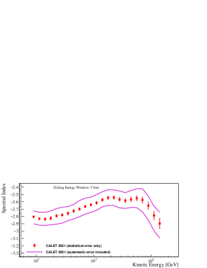
Figure 5 shows the energy dependence of the spectral index calculated within
a sliding energy window (red squares). The spectral index is determined for each bin by
a fit to the data including the neighboring 2 bins in the region below 20 TeV
above which the highest two bins have relatively large errors.
Magenta curves indicate the uncertainty band including systematic errors.
As the hardening is very gradual, its onset (around 200 GeV) can be read off directly from Figure 5. It is followed by a sharp softening of the flux above TeV. The first spectral transition is found to be parameterized [Eq.(2)] by a relatively low value of , while the second (sharper) one corresponds to a higher value of with a large uncertainty. Both parameters are left free in the fit. The fitted value of is found to be anticorrelated with the parameter. We additionally performed an independent fit to and with single-power-law functions in three energy sub-intervals, as shown in the Supplemental Material CAL . They were found to be consistent, within the errors, with the values obtained with the DBPL fit.
We have measured the cosmic-ray proton spectrum covering 3 orders of magnitude in energy from 50 GeV to 60 TeV and characterized two spectral features in the high-energy CR proton flux with a single measurement in low earth orbit. Our new data extend the energy interval of our previous measurement Adriani et al. (2019a) while keeping a good consistency with our earlier result.
Our spectrum is not consistent with a single power law covering the whole range: (i) above a few hundred GeV we confirm our previous observation Adriani et al. (2019a) of a progressive spectral hardening, also reported by CREAM, PAMELA, AMS-02, and DAMPE; (ii) at energies around 10 TeV we observe a second spectral feature with a softening starting around 10 TeV.
In this energy region the shape of the spectrum is consistent, within the errors, with the measurement reported by DAMPE. The results from two independent CALET analyses, with different efficiencies, were cross-checked and found in agreement.
Extended CALET operations were approved by JAXA/NASA/ASI in March 2021 through the end of 2024 (at least).
Improved statistics and refinement of the analysis, with additional data collected during the live time of the mission, will allow us to extend the proton measurement at higher energies and to reduce the systematic uncertainties.
We gratefully acknowledge JAXA’s contributions to the development of CALET and to the
operations onboard the International Space Station. We also express our sincere gratitude to ASI and NASA for
their support of the CALET project.
This work was supported in part by JSPS Grant-in-Aid for Scientific Research (S) Grant No.19H05608,
and by the MEXT-Supported Program for the Strategic Research Foundation at Private Universities
(2011–2015) (Grant No.S1101021) at Waseda University.
The CALET effort in Italy is supported by ASI under Agreement No. 2013-018-R.0 and its amendments.
The CALET effort in the U.S. is supported by NASA through Grants
No. 80NSSC20K0397, No. 80NSSC20K0399, and No. NNH18ZDA001N-APRA18-004.
References
- Panov et al. (2007) A. Panov et al., Bull. Russ. Acad. Sci. Phys. 71, 494 (2007).
- Ahn et al. (2009) H. Ahn et al., Astrophys. J. 707, 593 (2009).
- Ahn et al. (2010) H. Ahn et al., Astrophys. J. Lett. 714, L89 (2010).
- Yoon et al. (2011) Y. Yoon et al., Astrophys. J. 728, 122 (2011).
- Adriani et al. (2011) O. Adriani et al., Science 332, 69 (2011).
- Aguilar et al. (2015a) M. Aguilar et al. (AMS Collaboration), Phys. Rev. Lett. 114, 171103 (2015a).
- Aguilar et al. (2015b) M. Aguilar et al. (AMS Collaboration), Phys. Rev. Lett. 115, 211101 (2015b).
- Yoon et al. (2017) Y. Yoon et al., Astrophys. J. 839, 5 (2017).
- Aguilar et al. (2017) M. Aguilar et al. (AMS Collaboration), Phys. Rev. Lett. 119, 251101 (2017).
- Aguilar et al. (2018a) M. Aguilar et al. (AMS Collaboration), Phys. Rev. Lett. 120, 021101 (2018a).
- Aguilar et al. (2018b) M. Aguilar et al. (AMS Collaboration), Phys. Rev. Lett. 121, 051103 (2018b).
- Adriani et al. (2019a) O. Adriani et al. (CALET Collaboration), Phys. Rev. Lett. 122, 181102 (2019a).
- Adriani (2019) O. Adriani et al. (CALET Collaboration), Phys. Rev. Lett. 125, 251102 (2020).
- (14) M. Aguilar et al. (AMS Collaboration), Phys. Rev. Lett. 124, 211102 (2020).
- Ellison et al. (1997) D. Ellison et al., Astrophys. J. 487, 197 (1997).
- Malkov et al. (2012) M. A. Malkov, P. H. Diamond, and R. Z. Sagdeev, Phys. Rev. Lett. 108, 081104 (2012).
- Erlykin and Wolfendale (2012) A. Erlykin and A. Wolfendale, Astropart. Phys. 35, 449 (2012).
- Drury (2011) L. Drury, Mon. Not. R. Astron Soc. 415, 1807 (2011).
- Ohira et al. (2016) Y. Ohira, N. Kawanaka, and K. Ioka, Phys. Rev. D 93, 083001 (2016).
- Biermann et al. (2010) P. Biermann et al., Astrophys. J. 725, 184 (2010).
- Ptuskin et al. (2013) V. Ptuskin, V. Zirakashvili, and E. Seo, Astrophys. J. 763, 47 (2013).
- Zatsepin and Sokolskaya (2006) V. Zatsepin and N. Sokolskaya, Astron. Astrophys. 458, 1 (2006).
- Vladimirov et al. (2012) A. Vladimirov, G. Jóhannesson, I. Moskalenko, and T. Porter, Astrophys. J. 752, 68 (2012)NoStop
- Kawanaka and Yanagita (2018) N. Kawanaka and S. Yanagita, Phys. Rev. Lett. 120, 041103 (2018).
- Blasi et al. (2012) P. Blasi, E. Amato, and P. D. Serpico, Phys. Rev. Lett. 109, 061101 (2012).
- Aloisio and Blasi (2013) R. Aloisio and P. Blasi, J. Cosmol. Astropart. Phys. 07 (2013) 001.
- Thoudam and Hörandel (2014) S. Thoudam and J. Hörandel, Astron. Astrophys. 567, A33 (2014).
- Tomassetti (2012) N. Tomassetti, Astrophys. J. Lett. 752, L13 (2012).
- Tomassetti (2015) N. Tomassetti, Phys. Rev. D 92, 063001 (2015).
- Giacinti et al. (2018) G. Giacinti, M. Kachelrieß, and D. Semikoz, J. Cosmol. Astropart. Phys. 07 (2018) 051.
- Evoli et al. (2018) C. Evoli, P. Blasi, G. Morlino, and R. Aloisio, Phys. Rev. Lett. 121, 021102 (2018).
- Thoudam and Hörandel (2012) Thoudam and J. Hörandel, Mon. Not. R. Astron Soc. 421, 1209 (2012).
- Bernard et al. (2013) G. Bernard et al., Astron. Astrophys. 555, A48 (2013).
- Lipari (2021) P. Lipari, Proc. Sci., ICRC2021 (2021) 169.
- Recchia (2021) S. Recchia, Proc. Sci., ICRC2021 (2021) 168.
- (36) D. Caprioli, C. Haggerty, and P. Blasi, Proc. Sci., ICRC2021 (2021) 482.
- (37) P. Cristofari, P. Blasi, and E. Amato, Proc. Sci., ICRC2021 (2021) 151.
- Morlino (2021) G. Morlino, Proc. Sci., ICRC2021 (2021) 444.
- (39) Q. An et al. (DAMPE Collaboration), Sci. Adv. 5, eaax3793 (2019).
- K. Kobayashi and P.S. Marrocchesi (2021) K. Kobayashi and P.S. Marrocchesi (CALET Collaboration), Proc. Sci., ICRC2021 (2021) 098.
- Atkin et al. (2018) E. Atkin et al., JETP Lett. 108, 5 (2018).
- (42) Y. S. Yoon et al. (CREAM-III Collaboration), Astrophys. J 839, 5 (2017).
- Marrocchesi (2021) P. S. Marrocchesi (CALET Collaboration), Proc. Sci., ICRC2021 (2021) 010.
- Asaoka et al. (2018) Y. Asaoka, Y. Ozawa, S. Torii, et al. (CALET Collaboration), Astropart. Phys. 100, 29 (2018).
- Adriani et al. (2017a) O. Adriani et al. (CALET Collaboration), Phys. Rev. Lett. 119, 181101 (2017a).
- Adriani et al. (2018) O. Adriani et al. (CALET Collaboration), Phys. Rev. Lett. 120, 261102 (2018).
- P. Brogi and K.Kobayashi (2021) P. Brogi and K. Kobayashi (CALET Collaboration), Proc. Sci., ICRC2021 (2021) 101.
- (48) P. Maestro (CALET Collaboration), Proc. Sci. ICRC2021 (2021) 093 (2021).
- Y.Akaike and Y.Akaike (2021) Y. Akaike and P. Maestro (CALET Collaboration), Proc. Sci., ICRC2021 (2021) 112.
- Adriani et al. (2018) O. Adriani et al. (CALET Collaboration), Phys. Rev. Lett. 126, 241101 (2021).
- F.Stolzi, C.Checchia and C.Checchia (2021) F. Stolzi, C. Checchia and Y. Akaike (CALET Collaboration), Proc. Sci., ICRC2021 (2021) 109.
- Adriani et al. (2018) O. Adriani et al. (CALET Collaboration), Phys. Rev. Lett. 128, 131103 (2022).
- (53) W.V. Zober, B.F. Rauch and A.W. Ficklin (CALET Collaboration), Proc. Sci., ICRC2021 (2021) 124.
- Torii (2019) S. Torii (CALET Collaboration), Proc. Sci., ICRC2019 (2019) 142.
- (55) P. S. Marrocchesi et al., Nucl. Instrum. Methods Phys. Res., Sect. A 659, 477 (2011).
- (56) P. S. Marrocchesi (CALET Collaboration), Proc. Sci., ICRC2019 (2019) 103.
- (57) P. Brogi et al. (CALET Collaboration), Proc. Sci., ICRC2015 (2015) 595.
- Asaoka et al. (2017) Y. Asaoka, Y. Akaike, Y. Komiya, R. Miyata, S. Torii et al. (CALET Collaboration), Astropart. Phys. 91, 1 (2017).
- Kasahara (1995) K. Kasahara, in Proc. of 24th International Cosmic Ray Conference (Rome, Italy) (1995) Vol. 1, p. 399.
- (60) EPICS and COSMOS versions are 9.20 and 8.00, respectively .
- Böhlen (2014) T. Böhlen, Nucl. Data Sheets 120, 211 (2014).
- Ferrari et al. (2005) A. Ferrari et al., Report Nos. INFN/TC_05/11, SLAC-R-773, CERN-2005-10, Istituto Nazionale di Fisica Nucleare (INFN), Stanford Linear Accelerator Center (SLAC), CERN (European Organization for Nuclear Research) 2005.
- (63) The version of FLUKA is Fluka2011.2c.4.
- Agostinelli et al. (2003) S. Agostinelli et al., Nucl. Instrum. Methods Phys. Res., Sect. A 506, 250 (2003).
- (65) Geant4 version with FTFP_BERT as a physics list recommended for the simulation of high energy showers .
- Maestro et al. (2017) P. Maestro, N. Mori et al. (CALET Collaboration), Proc. Sci., ICRC2017 (2017) 208.
- (67) See Supplemental Material at http://link.aps.org/supplemental/10.1103/PhysRevLett.129.101102 for supporting figures and the tabulated proton flux, as well as the description of data analysis procedure and the detailed assessment of systematic uncertainties.
- Adye (2011) T. Adye, Proceedings of the PHYSTAT 2011 Workshop (CERN, Geneva, 2011).
- D’Agostini (1995) G. D’Agostini, Nucl. Instrum. Methods Phys. Res., Sect. A, 362, 487 (1995).
- Brun and Rademakers (1997) R. Brun and F. Rademakers, Nucl. Instrum. Methods Phys Res., Sect. A, 389, 81 (1997).