Accelerating Polynomial Multiplication for Homomorphic Encryption on GPUs

Abstract

Homomorphic Encryption (HE) enables users to securely outsource both the storage and computation of sensitive data to untrusted servers. Not only does HE offer an attractive solution for security in cloud systems, but lattice-based HE systems are also believed to be resistant to attacks by quantum computers. However, current HE implementations suffer from prohibitively high latency. For lattice-based HE to become viable for real-world systems, it is necessary for the key bottlenecks—particularly polynomial multiplication—to be highly efficient.

In this paper, we present a characterization of GPU-based implementations of polynomial multiplication. We begin with a survey of modular reduction techniques and analyze several variants of the widely-used Barrett modular reduction algorithm. We then propose a modular reduction variant optimized for $64$-bit integer words on the GPU, obtaining a $1.8\times$ speedup over the existing comparable implementations. Next, we explore the following GPU-specific improvements for polynomial multiplication targeted at optimizing latency and throughput: 1) We present a 2D mixed-radix, multi-block implementation of NTT that results in a $1.85\times$ average speedup over the previous state-of-the-art. 2) We explore shared memory optimizations aimed at reducing redundant memory accesses, further improving speedups by $1.2\times$. 3) Finally, we fuse the Hadamard product with neighboring stages of the NTT, reducing the twiddle factor memory footprint by $50\%$. By combining our NTT optimizations, we achieve an overall speedup of $123.13\times$ and $2.37\times$ over the previous state-of-the-art CPU and GPU implementations of NTT kernels, respectively.

I Introduction

Computation is increasingly outsourced to remote cloud-computing services [1, 2]. Encryption provides security as data is transmitted over the internet. However, classical encryption schemes require that data be decrypted prior to performing computation, exposing sensitive data to untrusted cloud providers [3, 4]. Using Homomorphic Encryption (HE) allows computations to be run directly on encrypted operands, offering ideal security in the cloud-computing era (Figure 1). Moreover, many of the breakthrough HE schemes are lattice-based, and are believed to be resistant to attacks by quantum computers [5].

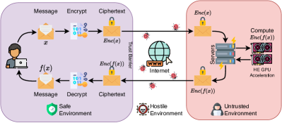
Figure 1: HE provides security from eavesdroppers on the web as well as untrusted cloud services, as encrypted data can be computed on directly.

One major challenge in deploying HE in real-world systems is overcoming the high computational costs associated with HE. For computation on data encrypted via state-of-the-art HE schemes—such as HE for Arithmetic of Approximate Numbers [6] (also known as HEAAN or CKKS) and TFHE [7]— a slowdown of 4–6 orders of magnitude is reported, as compared to running the same computation on unencrypted data [8, 9]. We aim to accelerate HE by targeting the main operation in these schemes (and, more generally, in lattice-based cryptography): polynomial multiplication [10, 11, 12]. The Number Theoretic Transform (NTT) and modular reduction are two key bottlenecks in polynomial multiplication (and, by extension, in HE), as evidenced by the performance profiling of several lattice-based cryptographic algorithms by Koteshwara et al. [13]. As lattice-based HE schemes have continued to establish themselves as leading candidates for privacy-preserving computing and other applications, there has been an increased focus on optimization and acceleration of these core operations [14, 15, 16].

For most real-world applications of lattice-based HE, the number $N$ of polynomial coefficients and the modulus $Q$ need to be large to guarantee a strong level of security and a higher degree of parallelism [9]. For example, $N=2^{16}$ and $\lceil{\log_{2}(Q)}\rceil=1240$ are the default values in the HEAAN library. The large values for $N$ and $Q$ translate to heavy workload demands, requiring a significant amount of computational power to evaluate modular arithmetic expressions, as well as placing high demands on the memory bandwidth utilization. HE workloads possess high levels of data parallelism [17]. Existing compute systems such as general-purpose CPUs do not scale well since they are unable to fully exploit this parallelism for such data-intensive workloads. However, the SIMD-style GPU platforms, with their thousands of cores and high bandwidth memory (HBM), are natural candidates for accelerating these highly parallelizable workloads. The potential of the GPU platform to accelerate HE has motivated a rapidly growing body of work over the past year [9, 18, 19, 20, 21, 22, 23, 24, 25, 26].

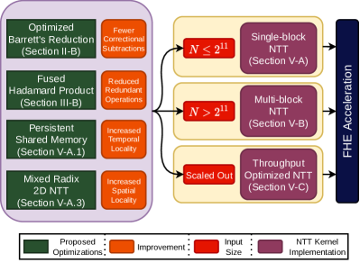
Figure 2: Our contributions: $4$ major optimizations incorporated into $3$ kernels

To address performance bottlenecks in existing polynomial multiplication algorithms, we begin by analyzing the Barrett modular reduction algorithm [27], as well as the algorithm’s variants [21, 26, 28] which have been utilized in prior HE schemes. We then analyze various NTT implementations, including mixed-radix and 2D implementations, which we tune to improve memory efficiency. Finally, we apply a number of GPU-specific optimizations to further accelerate HE. By combining all our optimizations, we achieve an overall speedup of $123.13\times$ and $2.37\times$ over the previous state-of-the-art CPU [29] and GPU [21] implementations of NTT kernels, respectively. Our key contributions are as follows (Figure 2):

1. We propose an instantiation of the Dhem–Quisquater [28] class of Barrett reduction variants which is optimized for HE, providing a $1.85\times$ speedup over prior studies [21, 23, 26, 30].

2. We present a mixed-radix, 2D NTT implementation to effectively exploit temporal and spatial locality, resulting in a $1.91\times$ speedup over the radix-2 baseline.

3. We propose a fused polynomial multiplication algorithm, which fuses the Hadamard product with its neighboring butterfly operations using an application of Karatsuba’s Algorithm [31]. This reduces the twiddle factor’s memory footprint size by $50\%$.

4. We incorporate the use of low latency, persistent, shared memory in our single-block NTT GPU kernel implementation, reducing the number of redundant data fetches from global memory, providing a further $1.25\times$ speedup.

II Barrett reduction and its variants

Modular reduction is a key operation and computational bottleneck in lattice-based cryptography [32]. This section is a self-contained survey of modular reduction algorithms, particularly Barrett reduction [27], a widely-used algorithm that we utilize in our work.

Following Shoup [33], we define the bit length $\mathrm{len}(a)$ of a positive integer $a$ to be the number of bits in the binary representation of $a$; more precisely, $\mathrm{len}(a)=\lfloor{\log_{2}a}\rfloor+1$.

II-A Background: modular reduction and arithmetic

Let $x\ \mathrm{mod}\ q$ denote the remainder of a nonnegative integer $x$ divided by a positive integer $q$. The naive method for performing modular reduction—i.e., the computation of $x\ \mathrm{mod}\ q$—is via an integer division operation:

$$x\ \mathrm{mod}\ q=x-\lfloor{x/q}\rfloor q.$$

However, there are a number of alternative methods for performing modular reduction—especially in conjunction with arithmetic operations such as addition and multiplication—that avoid expensive integer division operations.

For example, Algorithm 1 specifies a simple and efficient computation of the modular reduction of a sum. Let $\upbeta$ denote the word-size (e.g., $\upbeta=32$ or $64$). Observe that either $a+b$ lies in $[0,q)$ and is reduced, or $a+b$ lies in $[q,2q)$ and requires a single correctional subtraction to become reduced (see lines 2–3). The restriction $\mathrm{len}(q)\leq\upbeta-1$ prevents overflow of the transient operations (i.e., $a+b$).

Algorithm 1 A baseline modular addition algorithm

0:  $0\leq a,b<q$, $\mathrm{len}(q)\leq\upbeta-1$

0:  $\mathrm{sum}=(a+b)\ \mathrm{mod}\ q$

1:  $\mathrm{sum}\leftarrow a+b$

2:  if $\mathrm{sum}\geq q$ then

3:     $\mathrm{sum}\leftarrow\mathrm{sum}-q$

4:  return  $\mathrm{sum}$

There are multiple methods for reducing products. In lattice-based cryptography, commonly used algorithms for implementations on hardware platforms such as CPUs and GPUs include the algorithms of Barrett [27], Montgomery [34], and Shoup [35, 36]. In this paper, we select Barrett’s algorithm as our baseline, as Barrett’s algorithm enjoys the following features:

1. Low overhead: It requires a low-cost pre-computation (and storage) of a single word-size integer $\mu$.

2. Versatility: It may be used effectively in contexts where multiple products are reduced modulo $q$.

3. Generality: It does not restrict to special classes of moduli, such as Mersenne primes (see, e.g., [37, 38]).

4. Performant: It is significantly faster than integer division, and has comparable runtime performance with Montgomery’s algorithm (see, e.g., [39]).

Barrett’s algorithm is used in many open-source libraries, including cuHE [40], PALISADE [41], and HEANN [20, 6]. The Barrett reduction algorithm, and our proposed variant for use in HE, are analyzed in Section II-B.

II-B Barrett modular reduction: analysis and optimization

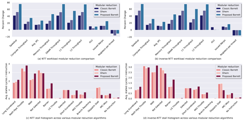
Figure 3: Modular reduction profile comparison of architectural parameters (a,b) and causes of warp stalls (c,d).

Next, we provide details of Barrett modular reduction and then explore potential improvements. Algorithm 2 specifies the classical reduction algorithm of Barrett [27].

Algorithm 2 Classical Barrett reduction

0:  $m=\mathrm{len}(q)\leq\upbeta-2$, $0\leq x<2^{2m}$, $\mu=\lfloor{\frac{2^{2m}}{q}}\rfloor$

0:  $\mathrm{rem}=x\ \mathrm{mod}\ q$

1:  $c\leftarrow x\gg(m-1)$

2:  $\mathrm{quot}\leftarrow(c\times\mu)\gg(m+1)$

3:  $\mathrm{rem}\leftarrow x-\mathrm{quot}\times q$

4:  if $\mathrm{rem}\geq q$ then

5:     $\mathrm{rem}\leftarrow\mathrm{rem}-q$

6:  if $\mathrm{rem}\geq q$ then

7:     $\mathrm{rem}\leftarrow\mathrm{rem}-q$

8:  return  $\mathrm{rem}$

Note that if $0\leq a,b<q$ and $m=\mathrm{len}(q)$, then $x=a\times b$ satisfies the condition $0\leq x<2^{2m}$ specified in Algorithm 2. This algorithm is commonly used in HE acceleration studies targeting a GPU [24, 30, 23, 42]. As noted by Sahu et al. [23], the pre-computed constant $\mu$ and the transient operations (excluding the product $c\times\mu$) are preferably word-sized. This condition imposes the restriction $\mathrm{len}(q)\leq\upbeta-2$.

Note that the classical Barrett reduction may require zero, one, or two correctional subtractions; see lines 4–7 in Algorithm 2. As noted by Barrett [27], a second conditional subtraction is required in approximately 1% of the cases. There have been several attempts to modify Barrett’s algorithm to eliminate the need for a second conditional subtraction. The algorithms proposed by Özerk et al. [21] and Lee et al. [26] each require two correctional subtractions to fully reduce the product of $a=994674970$ and $b=994705408$ modulo $q=994705409$, although we found experimentally that Özerk et al.’s proposed reduction algorithm only requires a second conditional subtraction in $0.22\%$ of cases.

Dhem–Quisquater [28] defines a class of Barrett modular reduction variants (with parameters $\alpha$ and $\beta$) that require at most one correctional subtraction. A commonly used (see, e.g., Kong and Philips [43] and Wu et al. [44]) instantiation of Dhem–Quisquater’s class of algorithms is specified in Algorithm 3 (setting parameters $\alpha=N+3$ and $\beta=-2$, as defined in Dhem–Quisquater [28]). Notably, this instantiation is used in the PALISADE HE Software Library [41].

Algorithm 3 Dhem–Quisquater’s modified Barrett reduction

0:  $m=\mathrm{len}(q)\leq\upbeta-4$, $0\leq x<2^{2m}$, $\mu=\lfloor{\frac{2^{2m+3}}{q}}\rfloor$

0:  $\mathrm{rem}=x\ \mathrm{mod}\ q$

1:  $c\leftarrow x\gg(m-2)$

2:  $\mathrm{quot}\leftarrow(c\times\mu)\gg(m+5)$

3:  $\mathrm{rem}\leftarrow x-\mathrm{quot}\times q$

4:  if $\mathrm{rem}\geq q$ then

5:     $\mathrm{rem}\leftarrow\mathrm{rem}-q$

6:  return  $\mathrm{rem}$

Although Algorithm 3 provides an improvement in algorithmic complexity over Algorithm 2, it further restricts the modulus to at most length $(\upbeta-4)$ to ensure $\mu$ is word-sized.

As discussed by Kim et al. [20], restrictions on the modulus size are significant in the context of optimizing HE, as the modulus size is inversely related to the workload size. To elaborate, polynomial multiplication is typically performed with respect to a large composite modulus $Q$. If each prime factor of $Q$ is $m$-bits, then the Chinese Remainder Theorem can be used to partition the computation of polynomial multiplication with respect to $Q$ into $\lceil{\mathrm{len}(Q)/m}\rceil$ simpler computations of polynomial multiplication with respect to the $m$-bit factors. For example, if $\mathrm{len}(Q)=1240$, then the restriction from 30-bit to 28-bit moduli increases the workload size (i.e., $\lceil{\mathrm{len}(Q)/m}\rceil$) by $7.14\%$.

Therefore, we propose Algorithm 4 for use in HE implementations on a GPU. Similar to Algorithm 3, Algorithm 4 is an instantiation of Dhem–Quisquater [28] (for $\alpha=N+1$ and $\beta=-2$) that requires at most one correctional subtraction. However, Algorithm 4 allows for moduli $q$ of length up to $\upbeta-2$, and thus results in no increase in the workload size.

Algorithm 4 Proposed Barrett reduction optimized for a GPU

0:  $m=\mathrm{len}(q)\leq\upbeta-2$, $0\leq x<2^{2m}$, $\mu=\lfloor{\frac{2^{2m+1}}{q}}\rfloor$

0:  $\mathrm{rem}=x\ \mathrm{mod}\ q$

1:  $c\leftarrow x\gg(m-2)$

2:  $\mathrm{quot}\leftarrow(c\times\mu)\gg(m+3)$

3:  $\mathrm{rem}\leftarrow x-\mathrm{quot}\times q$

4:  if $\mathrm{rem}\geq q$ then

5:     $\mathrm{rem}\leftarrow\mathrm{rem}-q$

6:  return  $\mathrm{rem}$

Figure 3 provides a snapshot of the performance of various modular reduction kernels on a V100 GPU. The detailed description of each parameter is further described in Table I and II in Section IV. The values in the Figure 3(a,b) are normalized to the built-in implementation of modular reduction on GPUs (which utilizes the modulo “$\%$” operator). In Figure 3(a,b) we see significant improvements in the proposed Barrett reduction, as marked by the speedups due to improved compute and memory throughput. The performance improvements achieved can be attributed to our implementation requiring at most $1$ correctional subtraction (as compared to $2$ for others). Figure 3(c,d) enable us to see the primary causes of kernel stalls for NTT and inverse-NTT workloads, respectively. Figure 3(c,d) highlights the reasons for the maximum number of stalls while executing NTT and inverse-NTT kernels. In Figure 3(c), the longest stall (measured in the average number of cycles per instruction) for the NTT workload is due to a “Math Pipe Throttle”, which results when the kernel begins to saturate the ALU instruction pipeline (See Table I). Figure 3(d) reports the cause of stalls in inverse-NTT, with the longest stall caused by a “Wait”, which signifies the scheduler has an abundance of “Ready” warps and is starting to saturate the streaming multiprocessors (SMs) (See Table II).

In Figure 4, we present a comparison of the implementations of the modular reduction algorithms described in this section. We report the execution time of a single modular reduction operation for 28, 29, and 30-bit prime numbers as run on a V100 GPU. The operands and moduli are randomly sampled from a uniform distribution. The classical Barrett reduction algorithm is significantly faster than reduction by integer division (i.e., the built-in reduction), as shown in Figure 4. Algorithm 4 has nearly identical performance to Algorithm 3 for 28-bit moduli (while permitting 29 and 30-bit moduli, as well). Algorithm 4 has a $1.22\times$ speedup over the classical Barrett reduction for 30-bit primes. To our knowledge, the specific instantiation of Dhem–Quisquater modular reduction specified in Algorithm 4 does not appear in an open-source library nor in the literature.

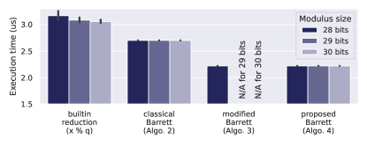
Figure 4: Execution times of modular reduction implementations for $28$, $29$, and $30$-bit prime numbers (on the V100 GPU), averaged over 10,000 iterations. The error bars represent ranges. The “builtin reduction” uses the CUDA % construct for modular reduction.

III Polynomial Multiplication

For $m>0$, define $\mathbb{Z}_{m}$ to be the set $\{0,1,2,\ldots,m-1\}$ together with the operations of modular addition $(a,b)\mapsto(a+b)\ \mathrm{mod}\ m$ and modular multiplication $(a,b)\mapsto(a\times b)\ \mathrm{mod}\ m$. The naive algorithm for multiplying two polynomials $\sum_{i=0}^{N-1}a_{i}x^{i}$ and $\sum_{i=0}^{N-1}b_{i}x^{i}$ requires order $N^{2}$ arithmetic operations. It is well known [45] that the number of operations can be reduced to the order of $N\log(N)$ using the Fast Fourier Transform (FFT) algorithm.

It is convenient to represent a polynomial $\sum_{i=0}^{N-1}a_{i}x^{i}$ as an $N$-dimensional coefficient vector ${\bf a}=(a_{0},a_{1},\ldots,a_{N-1})$.

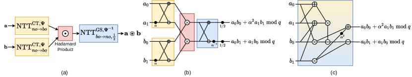
Figure 5: (a) Negacyclic convolution block diagram. (b) Hadamard product and its neighboring butterflies. (c) Fusion of butterflies into Hadamard product.

III-A Background: Number Theoretic Transform

In this section, we give a brief review of the Discrete Fourier Transform (DFT) and the Fast Fourier Transform (FFT) for the special case that the field of coefficients is $\mathbb{Z}_{q}$, for $q$ a prime. The DFT and FFT over $\mathbb{Z}_{q}$ are both commonly—and often confusingly—referred to as the Number Theoretic Transform (NTT). In the classical setup for the NTT, the parameters $N$, $q$, and $\omega$ satisfy the following properties:

1. $N>1$ is a power of $2$;

2. $q$ is a prime number such that $N$ divides $q-1$; and

3. $\omega$ is a primitive $N$th root of unity in $\mathbb{Z}_{q}$; i.e., $\omega^{i}=1$ if and only if $i$ is a multiple of $N$.

The $N$-point NTT (DFT) with respect to $\omega$ is the function $\mathrm{NTT}_{\omega}:(\mathbb{Z}_{q})^{N}\rightarrow(\mathbb{Z}_{q})^{N}$ defined by $\mathrm{NTT}_{\omega}({\bf a})=(\sum_{i=0}^{N-1}{\bf a}[i]\omega^{ij})_{j=0}^{N-1}$. The inverse transformation of $\mathrm{NTT}_{\omega}$ is $\frac{1}{N}\mathrm{NTT}_{\omega^{-1}}$. Famously, the cyclic convolution [46] of vectors ${\bf a}$ and ${\bf b}$ in $(\mathbb{Z}_{q})^{N}$ can be computed in the order of $N\log(N)$ arithmetic operations via the expression $\frac{1}{N}\mathrm{NTT}_{\omega^{-1}}(\mathrm{NTT}_{\omega}({\bf a})\odot\mathrm{NTT}_{\omega}({\bf b}))$, where $\odot$ denotes the Hadamard product (i.e., entry-wise multiplication) on $(\mathbb{Z}_{q})^{N}$.

A closely related operation to cyclic convolution is negacyclic convolution, which is widely known as polynomial multiplication in the context of lattice-based cryptography [47]. The setup for polynomial multiplication has parameters $N$, $q$, and $\psi$ satisfying the following properties:

1. $N>1$ is a power of $2$;

2. $q$ is a prime such that $2N$ is a divisor of $q-1$; and

3. $\psi$ is a primitive $2N$th root of unity in $\mathbb{Z}_{q}$ (which implies that $\omega=\psi^{2}$ is a primitive $N$th root of unity).

Let ${\bf\Psi}$ and ${\bf\Psi^{-1}}$ denote the vector of “twiddle factors” in $(\mathbb{Z}_{q})^{N}$, defined by ${\bf\Psi}[i]=\psi^{i}$ and ${\bf\Psi^{-1}}[i]=\psi^{-i}$ for all $i$. Then the negacyclic convolution ${\bf a}\circledast{\bf b}$ of vectors ${\bf a}$ and ${\bf b}$ in $(\mathbb{Z}_{q})^{N}$ satisfies the following relation [48]:

$${\bf a}\circledast{\bf b}={\bf\Psi^{-1}}\odot\frac{1}{N}\mathrm{NTT}_{\omega^{-1}}(\mathrm{NTT}_{\omega}({\bf\Psi}\odot{\bf a})\odot\mathrm{NTT}_{\omega}({\bf\Psi}\odot{\bf b}))$$

The NTT algorithm (i.e., the FFT) used to compute the NTT mathematical function (i.e., the DFT) consists of an iteration of stages, in which computations are performed in the form of butterfly operations. The computational graphs for the well-studied (radix-2) Cooley–Tukey (CT) butterfly [49] and the Gentleman–Sande (GS) butterfly [50] are shown in Figure 6.

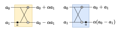
Figure 6: The Cooley–Tukey (left) and Gentleman–Sande butterflies (right).

Pöppelmann et al. [47] define an elegant algorithmic specification for polynomial multiplication using NTTs based on the CT and GS butterflies. Their design utilizes two specialized variants of the FFT/NTT:

1. the merged CT NTT, $\mathrm{NTT}^{\mathrm{CT},{\psi}}_{no\rightarrow bo}$, defined by Roy et al. [51] (see Algorithm 5); and

2. the merged GS NTT, $\mathrm{NTT}^{\mathrm{GS},{\psi}}_{bo\rightarrow no}$, defined by Pöppelmann et al. [47] (see Algorithm 6).

Algorithm 5 Merged CT NTT, $\mathrm{NTT}^{\mathrm{CT},{\psi}}_{no\rightarrow bo}$

0:  permuted twiddle factors ${\bf\Psi}_{\mathrm{br}}$

1:  $m\leftarrow 1$  

2:  $k\leftarrow N/2$

3:  while $m<N$ do

4:     for $i=0$ to $m-1$ do

5:        $jFirst\leftarrow 2\times i\times k$  

6:        $jLast\leftarrow jFirst+k-1$  

7:        $\xi\leftarrow{\bf\Psi}_{\mathrm{br}}[m+i]$  

8:        for $j=jFirst$ to $jLast$ do

9:           $\begin{bmatrix}{\bf a}[j]\\ {\bf a}[j+k]\end{bmatrix}\leftarrow\begin{bmatrix}{\bf a}[j]+\xi\times{\bf a}[j+k]\ \mathrm{mod}\ q\\ {\bf a}[j]-\xi\times{\bf a}[j+k]\ \mathrm{mod}\ q\end{bmatrix}$  

10:     $m\leftarrow 2\times m$  

11:     $k\leftarrow k/2$  

12:  return  ${\bf a}$

Algorithm 6 Merged GS NTT, $\mathrm{NTT}^{\mathrm{GS},{\psi}}_{bo\rightarrow no}$

0:  permuted twiddle factors ${\bf\Psi}_{\mathrm{br}}$

1:  $m\leftarrow N/2$  

2:  $k\leftarrow 1$

3:  while $m\geq 1$ do

4:     for $i=0$ to $m-1$ do

5:        $jFirst\leftarrow 2\times i\times k$  

6:        $jLast\leftarrow jFirst+k-1$  

7:        $\xi\leftarrow{\bf\Psi}_{\mathrm{br}}[m+i]$  

8:        for $j=jFirst$ to $jLast$ do

9:           $\begin{bmatrix}{\bf a}[j]\\ {\bf a}[j+k]\end{bmatrix}\leftarrow\begin{bmatrix}{\bf a}[j]+{\bf a}[j+k]\ \mathrm{mod}\ q\\ \xi\times({\bf a}[j]-{\bf a}[j+k])\ \mathrm{mod}\ q\end{bmatrix}$  

10:     $m\leftarrow m/2$  

11:     $k\leftarrow 2\times k$  

12:  return  ${\bf a}$

In Algorithms 5 and 6, $\mathrm{br}$ denotes the bit-reversal of a $\log_{2}(N)$-bit binary sequence, and ${\bf\Psi}_{\mathrm{br}}$ denotes the twiddle factors permuted with respect to $\mathrm{br}$; i.e., ${\bf\Psi}_{\mathrm{br}}[i]=\psi^{\mathrm{br}(i)}$ for all $i$ in $[0,N)$. Polynomial multiplication can be computed via the merged CT and GS NTTs as follows [47]:

$${\bf a}\circledast{\bf b}=\frac{1}{N}\mathrm{NTT}^{\mathrm{GS},{\psi^{-1}}}_{bo\rightarrow no}(\mathrm{NTT}^{\mathrm{CT},{\psi}}_{no\rightarrow bo}({\bf a})\odot\mathrm{NTT}^{\mathrm{CT},{\psi}}_{no\rightarrow bo}({\bf b})).$$ (1)

The advantages of this algorithmic specification for polynomial multiplication include the following:

1. Hadamard products omitted: The multiplication by powers of $\psi$, i.e., the Hadamard products with ${\bf\Psi}$ and ${\bf\Psi^{-1}}$, are “merged” into the NTT computations, saving a total of $3N$ modular multiplications.

2. Bit-reversal permutations omitted: The merged CT NTT takes the input in normal order and returns the output in a permuted bit-reversed order (hence $no\rightarrow bo$), and vice versa for the merged GS NTT. This removes the need for intermediate permutations to correct the order.

3. Good spatial locality: In the merged CT NTT, the twiddle factors ${\bf\Psi}_{\mathrm{br}}$ are read in sequential order. In the merged GS NTT, the twiddle factors are read sequentially during each stage.

Zhang et al. [52] propose a technique to merge the $\frac{1}{N}$-scaling operation in Equation (1) into the GS NTT. Rather than performing entry-wise modular multiplication by $\frac{1}{N}$, Zhang et al. multiply the output of each butterfly operation by $\frac{1}{2}$ modulo $q$. Observe that:

$$\frac{x}{2}\ \mathrm{mod}\ q=\begin{cases}\frac{x}{2}&\text{if $x$ is even}\\ \lfloor{\frac{x}{2}}\rfloor+\frac{q+1}{2}&\text{if $x$ is odd}\end{cases}$$

The computation of $\frac{x}{2}\ \mathrm{mod}\ q$ can be implemented without divisions, products, or branching via the expression

$$x\gg 1+(x\&1)\times((q+1)\gg 1).$$

Özerk et al. [21] use this technique to merge $\frac{1}{N}$-scaling into $\mathrm{NTT}^{\mathrm{GS},{\psi^{-1}}}_{bo\rightarrow no}$ (also see their open-source code [53]). We write $\mathrm{NTT}^{\mathrm{GS},{\psi{-1}}}_{bo\rightarrow no,\frac{1}{2}}$ to denote the merging of $\mathrm{NTT}^{\mathrm{GS},{\psi^{-1}}}_{bo\rightarrow no}$ with $\frac{1}{N}$-scaling. Incorporating this NTT into (1) gives the following algorithm specification for polynomial multiplication:

$${\bf a}\circledast{\bf b}=\mathrm{NTT}^{\mathrm{GS},{\psi^{-1}}}_{bo\rightarrow no,\frac{1}{2}}(\mathrm{NTT}^{\mathrm{CT},{\psi}}_{no\rightarrow bo}({\bf a})\odot\mathrm{NTT}^{\mathrm{CT},{\psi}}_{no\rightarrow bo}({\bf b}))$$ (2)

This algorithm specification is the basis for all of our implementations of polynomial multiplication.

III-B Proposed optimization: fused polynomial multiplication

Alkim et al. [54] propose several techniques for integrating the Hadamard product with its neighboring butterflies. They specify polynomial multiplication algorithms involving one, two, and three-stage integrations. These algorithms have significantly reduced complexity for the multiplication of two polynomials. However, the complexity of multiplying larger numbers of polynomials may be significantly increased, especially when more stages are integrated.

We propose a single-stage fused polynomial multiplication, which offers significant speedup for multiplying two polynomials at minimized cost for multiplying larger numbers of polynomials. Our proposal uses Karatsuba’s algorithm [31] to reduce the number of modular products by $N/2$ compared to the single-stage algorithm of Alkim et al. [54].

Consider the computational subgraph of Equation (2) induced by the final stages of $\mathrm{NTT}^{\mathrm{CT},{\psi}}_{no\rightarrow bo}$, the Hadamard product $\odot$, and the first stage of $\mathrm{NTT}^{\mathrm{GS},{\psi^{-1}}}_{bo\rightarrow no,\frac{1}{2}}$. Each of the $N/2$ connected components in this graph are of the form

$$\frac{1}{2}\mathrm{butt}_{\alpha^{-1}}^{\mathrm{GS}}\left(\mathrm{butt}_{\alpha}^{\mathrm{CT}}\left(\begin{bmatrix}a_{0}\\ a_{1}\end{bmatrix}\right)\odot\mathrm{butt}_{\alpha}^{\mathrm{GS}}\left(\begin{bmatrix}b_{0}\\ b_{1}\end{bmatrix}\right)\right)$$ (3)

for some twiddle factor $\alpha$ and inputs $a_{0},a_{1},b_{0}$, and $b_{1}$ (see Figure 5). Thus, the computation for each component consists of 5 (modular) product operations, 2 scaling by $\frac{1}{2}$ operations, 6 sum/difference operations, and $2$ memory accesses. The output of the computation in expression (3) is

$$\begin{bmatrix}a_{0}\times b_{0}+\alpha^{2}\times a_{1}\times b_{1}\ \mathrm{mod}\ q\\ a_{0}\times b_{1}+a_{1}\times b_{0}\ \mathrm{mod}\ q\end{bmatrix}$$ (4)

Algorithm 7 also computes expression (3), but requires 4 products, 0 scalings by $\frac{1}{2}$, 5 sums/differences, and $1$ memory access. This variation on Karatsuba’s Algorithm [31] relies on the fact that $a_{0}\times b_{1}+a_{1}\times b_{0}\ \mathrm{mod}\ q$ is equivalent to

$$(a_{0}+a_{1})\times(b_{0}+b_{1})-a_{0}\times b_{0}-a_{1}\times b_{1}\ \mathrm{mod}\ q.$$

We say that Algorithm 7 fuses the CT and GS butterflies into the Hadamard product.

Algorithm 7 Butterflies fused into the Hadamard product

0:  $\left[\begin{smallmatrix}a_{0}\\ a_{1}\end{smallmatrix}\right],\left[\begin{smallmatrix}b_{0}\\ b_{1}\end{smallmatrix}\right]\in(\mathbb{Z}_{q})^{2}$, twiddle factor $\alpha^{2}\in\mathbb{Z}_{q}$

0:  $\left[\begin{smallmatrix}c_{0}\\ c_{1}\end{smallmatrix}\right]\leftarrow\left[\begin{smallmatrix}a_{0}\times b_{0}+\alpha^{2}\times a_{1}\times b_{1}\ \mathrm{mod}\ q\\ a_{0}\times b_{1}+a_{1}\times b_{0}\ \mathrm{mod}\ q\end{smallmatrix}\right]$

1:  $prod1\leftarrow a_{0}\times b_{0}\ \mathrm{mod}\ q$  

2:  $prod2\leftarrow a_{1}\times b_{1}\ \mathrm{mod}\ q$  

3:  $sum1\leftarrow a_{0}+a_{1}\ \mathrm{mod}\ q$  

4:  $sum2\leftarrow b_{0}+b_{1}\ \mathrm{mod}\ q$  

5:  $prod3\leftarrow sum1\times sum2\ \mathrm{mod}\ q$  

6:  $prod4\leftarrow\alpha^{2}\times prod2\ \mathrm{mod}\ q$  

7:  $sum3\leftarrow prod1+prod4\ \mathrm{mod}\ q$  

8:  $sum4\leftarrow prod3-prod1\ \mathrm{mod}\ q$  

9:  $sum5\leftarrow sum4-prod2\ \mathrm{mod}\ q$  

10:  $\left[\begin{smallmatrix}c_{0}\\ c_{1}\end{smallmatrix}\right]\leftarrow\left[\begin{smallmatrix}sum3\\ sum5\end{smallmatrix}\right]$

11:  return  $\left[\begin{smallmatrix}c_{0}\\ c_{1}\end{smallmatrix}\right]$

To define the fused polynomial multiplication algorithm, we first define truncated versions of the CT and GS NTTs. Define the truncated CT NTT, $\mathrm{\widehat{NTT}}^{\mathrm{CT},{\psi}}_{no\rightarrow bo}$, to be the merged CT NTT with the final stage omitted (i.e., line 3 in Algorithm 5 is replaced with “while $m<(N/2)$ do”). Likewise, define the truncated GS NTT, $\mathrm{\widehat{NTT}}^{\mathrm{GS},{\psi}}_{bo\rightarrow no,\frac{1}{2}}$, to be the merged GS NTT with the first stage omitted (i.e., line 3 in Algorithm 6 is replaced with “while $m>1$ do”). Our proposed fused polynomial multiplication is specified in Algorithm 8.

Algorithm 8 Proposed fused polynomial multiplication

0:  ${\bf a},{\bf b}\in(\mathbb{Z}_{q})^{N}$, permuted twiddle factors ${\bf\Psi}_{\mathrm{br}}$

0:  ${\bf c}={\bf a}\circledast{\bf b}$

1:  ${\bf\widehat{a}}=\mathrm{\widehat{NTT}}^{\mathrm{CT},{\psi}}_{no\rightarrow bo}({\bf a})$  

2:  ${\bf\widehat{b}}=\mathrm{\widehat{NTT}}^{\mathrm{CT},{\psi}}_{no\rightarrow bo}({\bf b})$  

3:  for $i=0$ to $N/2-1$ do

4:     $u\leftarrow{\bf\widehat{a}}[2i]\times{\bf\widehat{b}}[2i]\ \mathrm{mod}\ q$  

5:     $v\leftarrow{\bf\widehat{a}}[2i+1]\times{\bf\widehat{b}}[2i+1]\ \mathrm{mod}\ q$  

6:     $w\leftarrow({\bf\widehat{a}}[2i]+{\bf\widehat{a}}[2i+1])\times({\bf\widehat{b}}[2i]+{\bf\widehat{b}}[2i+1])\ \mathrm{mod}\ q$  

7:     $y\leftarrow w-u\ \mathrm{mod}\ q$  

8:     ${\bf\widehat{c}}[2i+1]\leftarrow y-v\ \mathrm{mod}\ q$  

9:     $z\leftarrow v\times{\bf\Psi}_{\mathrm{br}}[\frac{N}{4}+\lfloor{\frac{i}{2}}\rfloor]\ \mathrm{mod}\ q$  

10:     if $i$ is even then

11:        ${\bf\widehat{c}}[2i]\leftarrow u+z\ \mathrm{mod}\ q$  

12:     else

13:        ${\bf\widehat{c}}[2i]\leftarrow u-z\ \mathrm{mod}\ q$  

14:  ${\bf c}\leftarrow\mathrm{\widehat{NTT}}^{\mathrm{GS},{\psi^{-1}}}_{bo\rightarrow no,\frac{1}{2}}({\bf\widehat{c}})$  

15:  return  ${\bf c}$

The benefits of our proposed fused polynomial multiplication algorithm include the following:

1. Fewer operations: $N/2$ fewer modular product operations, $N$ fewer scaling by $\frac{1}{2}$ operations, $N/2$ fewer sum/difference operations, and $N/2$ fewer memory accesses (but $N/4$ additional negations).

2. Number of twiddle factors halved: The second half of the entries in the twiddle factor arrays for each of the merged NTTs are not used in fused polynomial multiplication and can be omitted.

3. Re-use of recently-accessed twiddle factors: The twiddle factors read in the last stage of the truncated CT NTT are immediately re-used in the fused Hadamard product.

IV GPU Architecture

We implement our polynomial multiplication kernels targeting NVIDIA’s $7^{th}$ generation Volta GPU architecture, the V100 PCIe GPU with 16 GB onboard memory.

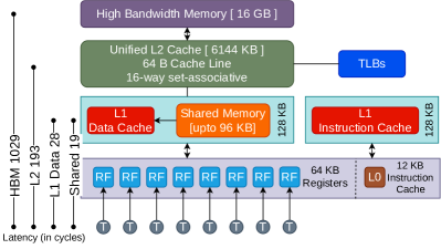
Figure 7: V100 GPU memory hierarchy and latency comparison.

The V100 has a multi-level memory, as shown in Figure 7. The V100 features a highly tuned high-bandwidth memory (HBM2), which is called global memory in the CUDA framework. The global memory, being the largest in capacity, has the highest latency to access data ($\mathtt{\sim}1029$ cycles) [55]. The V100 provides a $128$ KB L1 data cache and a $128$ KB L1 instruction cache per SM, as well as a unified L2 cache for data and instructions ($6.1$ MB in size). Each SM on a V100 has a shared memory (each configurable in size up to 96 KB). Data accesses to shared memory are much more efficient (i.e., $\mathtt{\sim}19$ cycles) as compared to accesses to global memory ($1029$ cycles) [56]. Effective use of the memory hierarchy, and especially shared memory, on a GPU is critical to obtaining the best performance [57]. Our single-block implementation of NTT utilizes shared memory for local data caching, thus reducing the number of redundant fetches from global memory [58] by a factor of $\log(N)$ times (where $N$ is the size of the input coefficient array). Furthermore, we improve cache efficiency by increasing the spatial locality of our data access patterns, exploiting memory coalescing on the GPU [58], as described in Section V-C.

We obtain performance metrics for our kernels using hardware performance counters and binary instrumentation tools. We explore performance bottlenecks using a variety of tools including the NVIDIA Binary Instrumentation Tool (NVBit) [59] for tracing memory transactions, the Nsight Compute for fetching performance counters, and the Nsight Systems [60] to obtain kernel scheduler performance, as well as measuring synchronization overheads. We compare kernel performance based on “Architectural Profile” and “Stall Profile” plots. The “Arch Profile” compares the relative change as compared to a baseline (see Table I), whereas the “Stall Profile” provides information on the primary causes of a kernel stall during execution (see Table II).

Parameter	Description
SM Throughput	% of cycles the SM was busy
Avg. IPC	Average # of instructions per cycle
ALU	ALU Pipeline utilization
DRAM B/W	% of peak memory transactions the DRAM processed per second
L1$ and L2$ B/W	% of peak memory transactions the L1$ and L2$ processed per second respectively
L1$ and L2$ Hit-Rate	% of memory transactions the L1$ and L2$ fulfilled successfully
Regs/Thread	# of registers used by each thread of the warp
Issued Warps	Avg. # of warps issued per second by scheduler

TABLE I: Description of the Arch Profile parameters.

Type of stall	Reason
Long Scoreboard	Waiting for a scoreboard dependency on a L1$ operation
Math Pipe Throttle	Waiting for the ALU execution pipe to be available
Wait	Waiting on fixed latency execution dependency Indicates highly optimized kernel
Not Selected	Waiting for the scheduler to select the warp Indicates warps oversubscribed to scheduler
Selected	Warp was selected by the micro scheduler
Barrier	Waiting for sibling warps at sync barrier Indicates diverging code paths before a barrier
LG Throttle	Waiting for the L1 instruction queue
Short Scoreboard	Scoreboard dependency on shared memory Indicates higher shared memory utilization
MIO Throttle	Stalled on MIO (memory I/O) instruction queue
Branch Resolving	Waiting for a branch target to be computed
Dispatch Stall	Warp stalled because dispatcher holds back issuing due to conflicts or events
IMC Miss	Waiting for an immediate cache (IMC) miss
No Instruction	Waiting after an instruction cache miss

TABLE II: Description of the Stall Profile parameters.

V Optimized NTT Kernels

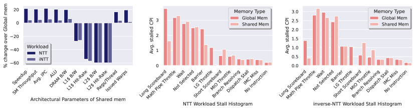
Figure 8: (a) Architectural performance profile of shared memory NTT and iNTT workloads compared against respective global memory workloads. (b) Stall profile of NTT workload comparing global and shared memory kernels. (c) Stall profile of inverse-NTT workload comparing global vs. shared memory kernels.

We observe that the NTT kernel is a memory-bound workload, heavily bottlenecked by the GPU’s DRAM latency. The butterfly operation is one of the key computations within the NTT kernel. This operation is characterized by strided accesses, with the stride varying with each stage. The changes in the stride lead to non-sequential memory accesses, reducing the spatial locality of the NTT kernel. To effectively leverage memory coalescing, we can partition data carefully across CUDA threads [61]. We propose three different implementations of NTT kernels, each optimized for different input sizes and employing different data partitioning techniques. We follow a similar approach here as described by Özerk et al. [21], though we leverage a number of algorithmic optimizations, combined with code optimizations, that are unique to this work.

The three implementations of polynomial multiplications proposed in this work are as listed below:

• LOS-NTT (Latency-optimized Single-block NTT): For single polynomial multiplication with $N~{}\leq~{}2^{11}$.

• LOM-NTT (Latency-optimized Multi-block NTT): For single polynomial multiplication with $N~{}>~{}2^{11}$.

• TOM-NTT (Throughput-optimized Multi-block NTT): For multiple polynomial multiplications with no constraints on $N$.

V-A Latency optimized Single-block NTT

The LOS-NTT kernel performs all the NTT operations within a single block of the CUDA kernel. Using a single block for computing the entire NTT workload has the following advantages:

• The overhead of a single block-level barrier ($syncthreads$) is significantly lower than a kernel-level (multi-block) barrier.

• We can leverage shared memory, which can only be addressed within the scope of a single block.

• Since all threads of a block share the same L1 and L2 caches, and L1 is write-through, write updates by any thread are reflected in L2 across all threads.

Our LOS-NTT implementation consists of two phases, separated by a block-level barrier. The first transfers the input coefficient vectors (of size $N$) from high latency global memory to the faster, low latency shared memory. The second phase performs the merged NTTs, as defined in Algorithms 5 and 6. This phase consists of two nested loops. The first iterates over the $\log(N)$ stages of the CT algorithm. This is followed by the second loop of $\frac{N}{2}$, iterating over the elements of the input coefficient vector. These iterations are free from any loop-carried dependencies, allowing them to be run in parallel. We capitalize on this inherent parallelism by computing each iteration of the second loop in parallel, assigning each loop iteration to a separate CUDA thread. We further improve the performance of our kernel with four GPU-specific optimizations.

V-A1 Shared Memory Optimization

Each stage of the CT implementation is characterized by multiple butterfly operations of varying strides. These butterfly operations result in strided memory accesses, with the step size varying from $1$ to $\frac{N}{2}$ (where $N$ can be as large as $2^{16}$). We optimize for memory access efficiency by storing the input coefficient vector, as well as the outputs of butterfly operations, in persistent shared memory, which is significantly faster than accessing global memory. We utilize $8$ KB of shared memory per SM for storing the input polynomial coefficients, as well as the output of intermediate stages. Using shared memory incurs the overhead of transferring input coefficients to shared memory and the final results back to global memory. Despite these additional overheads, incorporating the use of shared memory allows us to obtain a $1.25\times$ speedup over the use of only global memory (Figure 8). Figure 8(a) denotes a large drop in $L1\$$ and $L2\$$ performance. The primary reason for this degraded performance is memory transactions that access the shared memory do not count towards $L1$ and $L2$ cache performance. Since all the coalesced memory transactions to the global memory (which counted towards the cache performance) are now redirected towards the shared memory (which is excluded from cache performance counters), the $L1$ and $L2$ cache bandwidth and hit-rate take a performance hit. Figure 8(b,c) identifies the primary causes of stalls for the NTT and inverse-NTT kernels, respectively. The“Long Scoreboard” stall is caused by dependencies in L1 cache operations. The large drop in the stall values for the “Long Scoreboard” in Figure 8(b) is an indicator of memory pressure being reduced in the L1 cache and indirectly in the L2 cache and DRAM. Similarly, in Figure 8(c), the increase in the average “Math Pipe Throttle” stall values is tied to the compute throughput of the inverse-NTT kernel.

V-A2 Barrett’s Modular Reduction Optimization

We further accelerate our NTT kernel with the use of our modified Barrett implementation, specifically designed for GPU execution, as shown in Section II-B. The smaller number of correctional subtractions present in our implementation allows us to obtain a $1.85\times$ average speedup over previous work [21] and a $1.72\times$ speedup over the builtin modulus operation. We also obtain similar execution times to the $28$-bit modified Barrett’s reduction, as reported for PALISADE [41]. To our knowledge, our proposed Barrett variant is the fastest Barrett modular reduction for general $30$-bit and $62$-bit moduli.

V-A3 Mixed Radix Optimization

The naive implementation of NTT and inverse NTT used in this study is based on a radix-$2$ algorithm. In this implementation, each thread within a block operates on $2$ elements of the input coefficient array. We improve the performance of our kernel by experimenting with radix-$4$, $8$, and $16$ implementations that distribute $4$, $8$, and $16$ elements per thread, respectively. Higher radix implementations improve temporal locality, as the input coefficient vector data is reused. Unfortunately, this improvement in the temporal locality is associated with a significant loss in parallelism. We also experiment with kernels that use radix $4$ or radix $8$ for single-block kernels and radix $16$ for multi-block.

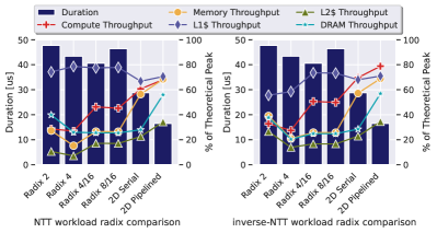
Figure 9: Higher radix comparison for (a) NTT and (b) inverse-NTT kernels.

We also experiment with $2$-dimensional NTT implementations. A 2D NTT maps the data into a matrix form, thus treating our coefficient as a row-major square matrix. This allows us to perform a column-wise NTT followed by a row-wise NTT. An $N-1$ degree polynomial can be mapped into a $\sqrt{N}\times\sqrt{N}$ matrix. This also divides the NTT kernel into two stages (column-wise NTT and row-wise NTT). The first stage computes $\sqrt{N}$ number of $\sqrt{N}$-point column-wise NTT operations, followed by the second stage that computes $\sqrt{N}$ number of $\sqrt{N}$-point row-wise NTT. Each $\sqrt{N}$-point NTT is mapped into a block with $\frac{\sqrt{N}}{2}$ threads, where each thread is responsible for computing a radix-$2$ butterfly. The 2D NTT approach allows us to map the data while preserving spatial locality. We further accelerate our computation by pipelining the two stages of row-wise and column-wise NTT operations, thus presenting two variants of our $2D$ implementation ($2D$ Serial and $2D$ Pipelined). This approach provides an average of $2.91\times$ speedup for NTT and inverse-NTT kernel over the naive radix-$2$ implementations (Figure 9). This improvement in execution time can be largely attributed to the increased memory throughput for NTT (Figure 9(a)), as well as inverse-NTT (Figure 9(b)). The improved memory throughput also contributes to the increased compute throughput, as continuous streaming of data from DRAM no longer starves the SMs of input operands.

V-A4 Fused Polynomial Multiplication Optimization

Finally, we propose an optimization that fuses together the last stage of merged CT NTT, the Hadamard product, and the first stage of merged GS NTT. Figure 5(c) shows the implementation of our fused polynomial multiplication. Our implementation of the fused kernel significantly reduces the number of multiplication operations and re-uses recently-cached twiddle factors. Experimental results show that we reduce the execution time, resulting in a $6.1\%$ and $2.4\%$ improvement as compared to the naive implementation for polynomial multiplication, for input sizes of $N=2^{11}$ and $N=2^{16}$, respectively.

V-B Latency optimized Multi-block NTT

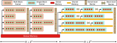
Figure 10: The Multi-block NTT task distribution.

The LOM-NTT kernel is designed to handle large input arrays ($N>2^{11}$). The LOM-NTT kernel distributes tasks using a similar strategy as used in the LOS-NTT kernel, except that it spreads them over multiple blocks. This allows us to employ multiple SMs to execute the workload in parallel. The LOM-NTT kernel splits a single $N$-point NTT between multiple blocks. Because of the use of multiple blocks, this implementation requires kernel-wide barriers for synchronization between stages. We use the LOM-NTT kernel to decompose a single $N$-point NTT into multiple $2^{11}$-point NTTs. Then we incorporate our LOS-NTT (Single-block) kernel to evaluate all the $2^{11}$-point NTTs to harness the optimizations of shared memory and block-level barriers. We show the distribution for our LOM-NTT for $N=2^{16}$ in Figure 10.

V-C Throughput-optimized Multi-block NTT

The throughput-optimized kernel is designed to compute multiple NTTs simultaneously. Unlike the latency-optimized kernel that computes just a single NTT operation, TOM-NTT is optimized to compute up to $2^{15}$ NTT operations simultaneously, with each NTT computation being a $2^{16}$-point NTT (the size of each input coefficient vector is $2^{16}$). The TOM-NTT kernel is fed $2$ input matrices. The first matrix holds the input coefficient vectors. These vectors, of size $2^{16}$, are stacked in the matrix in the row-major format. This matrix is then transferred to GPU and stored in global memory in a column-major format, coalescing reads across threads into a single memory transaction. The second input matrix contains the twiddle factors. We store twiddle factors in a similar way as the coefficient matrix. Each input matrix is of dimension $2^{16}\times 2^{15}$. Both matrices, when combined, completely fill the DRAM storage of $16$ GB on the V100 GPU. The TOM-NTT kernel executes the $2^{8}$-point NTT over $32,768$ vectors in $628~{}\mathrm{ms}$. With an average execution time is $19.17~{}\mu\mathrm{s}$ per NTT operation, this kernel exhibits close to linear weak scaling.

VI Results

VI-A Experimental Methodology

We present three different NTT kernels in this work, along with four optimizations tailored for the GPU platform. We evaluate the performance of our Single-block NTT kernel for input coefficient vector sizes of $N=2^{11}$ and of our Multi-block kernel for vector sizes of $N=2^{12}~{}\mathrm{to}~{}2^{16}$. We incrementally add each of the four optimizations to our NTT kernels and report performance improvements. Twiddle factors are pre-computed on the CPU and hence do not add to the compute overhead on the GPU. We report on multiple performance metrics for each approach, leveraging profiling tools on the GPU platform. For each optimization, the speedup achieved is reported using the respective non-optimized kernel as the baseline for comparison. Finally, we evaluate weak scaling for our throughput-optimized TOM-NTT kernel.

VI-B Performance Metrics

We incrementally add optimizations to our NTT kernels and report performance improvements in Table III (for input coefficient size $N=2^{16}$). For each optimization, the speedup achieved is reported, using the respective non-optimized kernel as the baseline for comparison.

Optimization	Relative Speedup	L1$ Throughput	DRAM Throughput
SM-only	$1.2\times$	$-27.3\%$	$+20.0\%$
SM + Alg4	$1.72\times$	$+10.86\%$	$+3.2\%$
SM + Alg4 + 2D	$2.91\times$	$+5.85\%$	$+16.14\%$
SM + Alg4 + 2D + FHP	$1.02\times$	$+0.3\%$	$-0.33\%$

TABLE III: NTT Kernel Optimizations: SM = shared memory, Alg4 = our proposed reduction, 2D = Mixed Radix 2D NTT, FHP = Fused Hadamard Product (NTT kernel with $N=2^{16}$ and $\lceil{\log_{2}(q)}\rceil=62$ used as baseline)

Our shared memory optimized kernel, when compared against the global memory kernel, achieves a $20\%$ improvement in DRAM bandwidth utilization and a $1.2\times$ speedup. Data is transferred between DRAM and shared memory using coalesced memory transactions, improving DRAM bandwidth utilization.

Next, we compare the execution time for our NTT kernel implementation by incorporating various modular reduction techniques, as shown in Figure 3. We compare our best performing NTT kernel (highlighted in Table IV) to Özerk et al. [21] and find a $1.85\times$ speedup for $N=2^{16}$ and a $1.13\times$ speedup for $N=2^{14}$. The use of radix $4$, $8$, and $16$ and $2D$ implementations provide additional speedup due to the increased temporal, as well as spatial, locality in $4$, $8$, and $16$-point butterfly operations, as compared to the baseline radix $2$ implementation. The effects of increased data locality are reflected in the $5.85\%$ improvement in the L1 cache hit-rate. Our best performing kernel, that of $2D$ NTT, achieves a $2.91\times$ speedup over a radix $2$ implementation (Figure 9). Our fused polynomial multiplication kernel reduced the execution time for the last stage of the merged CT NTT kernel, the Hadamard product, and the first stage of the merged GS NTT kernel, from $8.5~{}\mu\mathrm{s}$ down to $6.5~{}\mu\mathrm{s}$, resulting in a $1.3\times$ speedup as compared to its non-fused counterpart. When incorporated within a polynomial multiplication kernel, this translates to a $6.1\%$ improvement for Single-block kernel (for size $N=2^{11}$) and a $2.4\%$ improvement for Multi-block kernel (for size $N=2^{16}$).

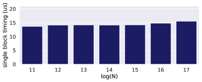
Figure 11: Timing for the Single-block NTT.

We also measured the scalability of our fastest single-block NTT implementation. As our multi-block kernel implementation leverages our Single-block code, we also analyzed the performance of the Single-block kernel by varying the input polynomial size and the hardware resources used. On each iteration, we double the size of the input array, as well as the number of potential SMs utilized (by doubling the number of blocks in the kernel). We observe that our Single-block kernel exhibits close to linear weak scaling, as execution times remain near constant as we increase both the input size and the hardware resources utilized (Figure 11).

We also evaluate our TOM-NTT kernel that is optimized for operating on a large number of NTT operations simultaneously (working with up to $2^{15}$ input coefficient vectors, each of size $2^{16}$ elements). With an average execution time of $19.17~{}\mu\mathrm{s}$ per NTT operation, this kernel exhibits close to linear weak scaling. Including all optimizations, our NTT kernels achieve a speedup of $123.13\times$ and $2.37\times$ over the previous state-of-the-art CPU [29] and GPU [21] implementations of NTT kernels, respectively.

VII Related Work

Table IV presents runtimes of various implementations of NTT and iNTT, adding to Table 8 in the work by Özerk et al. [21] with our own runtimes. Prior studies have explored accelerated NTT on FPGAs [62] and custom accelerators [8]. But these custom solutions are not typically found on general-purpose systems. On the other hand, GPUs are ubiquitous and easily programmed. In recent years, there has been growing interest in using a GPU to exploit the parallelism present in NTT [19, 20, 21]. In particular, Özerk et al. [21] propose an efficient hybrid kernel approach to accelerate NTT. Our LOS-NTT and LOM-NTT kernels are inspired by their work, however, we provide some further optimizations such as our fused Hadamard product, an improved version of Barrett reduction, and explored higher radix NTTs. Kim et al. [20] also propose some optimizations on NTTs, such as batching using shared memory. We explored how those optimizations could address the limitations we faced when implementing a kernel with a radix higher than 4.

Alkim et al. [54] define and analyze several algorithms very similar to Algorithm 8. They not only consider truncating their NTTs by one stage but by two and three stages. Although some of Alkim et al.’s algorithms utilize Karatsuba’s Algorithm, they do not consider using Karatsuba’s Algorithm to merge a single innermost pair of NTT stages. In our tests, our fused polynomial multiplication implementation provides an additional speedup of $6.1\%$ and $2.4\%$ as compared to the naive implementation for polynomial multiplication for input sizes of $N=2^{11}$ and $N=2^{16}$, respectively using Alkim et al.’s $(k-1)$-level NTT multiplication algorithm.

Work	Platform	$N$	$\lceil{\log_{2}(q)}\rceil$	NTT $(\mu s)$	iNTT $(\mu s)$
cuHE [40]∗	GTX $690$	$2^{14}$	$64^{c}$	$56$	$65.3$
		$2^{15}$	$64^{c}$	$71.2$	$83.6$
cuHE [40]∗,a	Tesla $K80$	$2^{14}$	$64^{c}$	$12.9$	$12.5$
		$2^{15}$	$64^{c}$	$19$	$21.6$
cuHE [40]∗,b	GTX $1070$	$2^{14}$	$64^{c}$	$66.8$	$-$
Faster NTT [63]∗	Tesla $K80$	$2^{14}$	$64^{c}$	$9.6$	$9.7$
		$2^{15}$	$64^{c}$	$15.3$	$16.2$
Accl NTT [24]∗	GTX $1070$	$2^{14}$	$64^{c}$	$57.8$	$-$
Bootstrap HE [20]	Titan $V$	$2^{14}$	$60$	$44.1$	$-$
		$2^{15}$	$60$	$84.2$	$-$
Re-encrypt [23]	GTX $1050$	$2^{14}$	NA	$255$	$-$
		$2^{15}$	NA	$470$	$-$
	RTX $1080$	$2^{14}$	NA	$375$	$-$
		$2^{15}$	NA	$425$	$-$
Efficient NTT [21]	GTX $980$	$2^{14}$	$55$	$51$	$41$
		$2^{15}$	$55$	$73$	$52$
	GTX $1080$	$2^{14}$	$55$	$33$	$20$
		$2^{15}$	$55$	$36$	$24$
	Tesla $V100$	$2^{14}$	$55$	$29$	$21$
		$2^{15}$	$55$	$39$	$23$
Our Work	Tesla $A100$	$2^{14}$	$62$	$13.3$	$10.9$
		$2^{16}$	$62$	$16.5$	$18.7$
	Tesla $V100$	$2^{14}$	$30$	$8.7$	$10.0$
		$2^{16}$	$30$	$13.1$	$13.4$
		$2^{14}$	$62$	$11.5$	$11.9$
		$2^{16}$	$62$	$\boldsymbol{16.4}$	$\boldsymbol{17.3}$

∗uses constant prime $q=\texttt{0xFFFFFFFF00000001}$

aresults are from [63]        bresults are from [24]

cactual $q_{i}$ is restricted by $q_{i}^{2}n<2^{64}-2^{32}+1$

TABLE IV: Comparison to related work

There is a Barrett reduction variant proposed by Yu et al. [64] that requires no correctional subtractions. We found that this algorithm has severe trade-offs in terms of operational complexity as a function of workload size, which makes it less attractive for use with HE.

VIII Conclusion

In this work, we presented an analysis and proposed implementations of polynomial multiplication, the key computational bottleneck in lattice-based HE systems, while targeting the V100 GPU platform. Specifically, we analyzed Barrett’s modular reduction algorithm and several variants. We studied the interplay between algorithmic improvements (such as multi-radix NTTs) and low-level kernel optimizations tailored towards the GPU (including memory coalescing). Our NTT optimizations achieve an overall speedup of $123.13\times$ and $2.37\times$ over the previous state-of-the-art CPU [29] and GPU [21] implementations of NTT kernels, respectively.

References

- [1] A. Ghosh and I. Arce, “Guest Editors’ Introduction: In Cloud Computing We Trust - But Should We?” IEEE Secur. Priv., vol. 8, no. 6, pp. 14–16, 2010. [Online]. Available: https://ieeexplore.ieee.org/stamp/stamp.jsp?arnumber=5655238
- [2] L. Branch, W. Eller, T. Bias, M. McCawley, D. Myers, B. Gerber, and J. Bassler, “Trends in malware attacks against United States healthcare organizations, 2016–2017,” Global Biosecurity, vol. 1, no. 1, 2019.
- [3] M. Jayaweera, K. Shivdikar, Y. Wang, and D. Kaeli, “JAXED: Reverse Engineering DNN Architectures Leveraging JIT GEMM Libraries,” in 2021 Int. Symp. on Secure and Private Execution Environ. Design (SEED). IEEE, 2021, pp. 189–202. [Online]. Available: https://wiki.kaustubh.us/w/img_auth.php/JAXED_Reverse_Engineering_DNN_Architectures_Leveraging_JIT_GEMM_Libraries.pdf
- [4] S. Thakkar, K. Shivdikar, and C. Warty, “Video steganography using encrypted payload for satellite communication,” in 2017 IEEE Aerospace Conf. IEEE, 2017, pp. 1–11. [Online]. Available: https://wiki.kaustubh.us/w/img_auth.php/Video_Steganography.pdf
- [5] E. L. Cominetti and M. A. Simplicio, “Fast additive partially homomorphic encryption from the approximate common divisor problem,” IEEE Trans. Inf. Forensics Secur., vol. 15, pp. 2988–2998, 2020.
- [6] J. H. Cheon, A. Kim, M. Kim, and Y. Song, “Homomorphic encryption for arithmetic of approximate numbers,” in Advances in Cryptology—ASIACRYPT 2017, T. Takagi and T. Peyrin, Eds. Springer, 2017.
- [7] I. Chillotti, N. Gama, M. Georgieva, and M. Izabachène, “TFHE: fast fully homomorphic encryption over the torus,” J. Cryptol., vol. 33, no. 1, pp. 34–91, 2020.
- [8] N. Samardzic, A. Feldmann, A. Krastev, S. Devadas, R. Dreslinski, C. Peikert, and D. Sanchez, “F1: A Fast and Programmable Accelerator for Fully Homomorphic Encryption,” in MICRO-54: 54th Annu. IEEE/ACM Int. Symp. on Microarchitecture, ser. MICRO ’21. New York, NY, USA: ACM, 2021, pp. 238–252.
- [9] W. Jung, E. Lee, S. Kim, J. Kim, N. Kim, K. Lee, C. Min, J. H. Cheon, and J. H. Anh, “Accelerating fully homomorphic encryption through architecture-centric analysis and optimization,” IEEE Access, vol. 9, pp. 98 772–98 789, 2021.
- [10] C. Gentry, “Fully homomorphic encryption using ideal lattices,” in Proc. of the 41st Annu. ACM Symp. on Theory of Comput.—STOC 2009. ACM, 2009, pp. 169–178.
- [11] V. Lyubashevsky, C. Peikert, and O. Regev, “On Ideal Lattices and Learning with Errors over Rings,” in Advances in Cryptology—EUROCRYPT 2010, H. Gilbert, Ed. Berlin, Heidelberg: Springer Berlin Heidelberg, 2010, pp. 1–23.
- [12] P. Longa and M. Naehrig, “Speeding up the number theoretic transform for faster ideal lattice-based cryptography,” in Int. Conf. on Cryptology and Netw. Security. Springer, 2016.
- [13] S. Koteshwara, M. Kumar, and P. Pattnaik, “Performance Optimization of Lattice Post-Quantum Cryptographic Algorithms on Many-Core Processors,” in 2020 IEEE Int. Symp. on Performance Anal. of Syst. and Softw. (ISPASS), 2020, pp. 223–225.
- [14] DARPA. (2021) DARPA Selects Researchers to Accelerate Use of Fully Homomorphic Encryption. [Online]. Available: https://www.darpa.mil/news-events/2021-03-08
- [15] A. Kim, M. Deryabin, J. Eom, R. Choi, Y. Lee, W. Ghang, and D. Yoo, “General bootstrapping approach for RLWE-based homomorphic encryption,” Cryptology ePrint Archive, 2021.
- [16] V. Kadykov and A. Levina, “Homomorphic properties within lattice-based encryption systems,” in 2021 10th Mediterranean Conf. on Embedded Comput. (MECO). IEEE, 2021, pp. 1–4.
- [17] P. Martins and L. Sousa, “Enhancing data parallelism of fully homomorphic encryption,” in Int. Conf. on Inf. Security and Cryptology. Springer, 2016, pp. 194–207.
- [18] W. Jung, S. Kim, J. H. Ahn, J. H. Cheon, and Y. Lee, “Over 100x faster bootstrapping in fully homomorphic encryption through memory-centric optimization with gpus,” IACR Transactions on Cryptographic Hardware and Embedded Syst., Aug. 2021.
- [19] Y. Zhai, M. Ibrahim, Y. Qiu, F. Boemer, Z. Chen, A. Titov, and A. Lyashevsky, “Accelerating Encrypted Computing on Intel GPUs,” 2022 IEEE Int. Parallel and Distrib. Process. Symp. (IPDPS), 2022.
- [20] S. Kim, W. Jung, J. Park, and J. H. Ahn, “Accelerating number theoretic transformations for bootstrappable homomorphic encryption on GPUs,” in 2020 IEEE Int. Symp. on Workload Characterization (IISWC), 2020.
- [21] Ö. Özerk, C. Elgezen, A. C. Mert, E. Öztürk, and E. Savaş, “Efficient number theoretic transform implementation on GPU for homomorphic encryption,” J. Supercomput., pp. 1–33, 2021. [Online]. Available: https://link.springer.com/content/pdf/10.1007/s11227-021-03980-5.pdf
- [22] S. Durrani, M. S. Chughtai, M. Hidayetoglu, R. Tahir, A. Dakkak, L. Rauchwerger, F. Zaffar, and W.-m. Hwu, “Accelerating fourier and number theoretic transforms using tensor cores and warp shuffles,” in Int. Conf. on Parallel Arch. and Compilation Tech. (PACT), 2021.
- [23] G. Sahu and K. Rohloff, “Accelerating Lattice Based Proxy Re-encryption Schemes on GPUs,” in Cryptology and Netw. Security, S. Krenn, H. Shulman, and S. Vaudenay, Eds. Springer, 2020.
- [24] J. Goey, W. Lee, B. Goi, and W. Yap, “Accelerating number theoretic transform in GPU platform for fully homomorphic encryption,” J. Supercomput., vol. 77, no. 2, pp. 1455–1474, 2021.
- [25] A. A. Badawi, B. Veeravalli, J. Lin, N. Xiao, M. Kazuaki, and A. K. M. Mi, “Multi-GPU Design and Performance Evaluation of Homomorphic Encryption on GPU Clusters,” IEEE Trans. Parallel Distrib. Syst., vol. 32, pp. 379–391, 2021.
- [26] W.-K. Lee, S. Akleylek, D. C.-K. Wong, W.-S. Yap, B.-M. Goi, and S.-O. Hwang, “Parallel implementation of Nussbaumer algorithm and number theoretic transform on a GPU platform: application to qTESLA,” J. Supercomput., vol. 77, no. 4, pp. 3289–3314, 2021.
- [27] P. Barrett, “Implementing the Rivest Shamir and Adleman Public Key Encryption Algorithm on a Standard Digital Signal Processor,” in Advances in Cryptology — CRYPTO’ 86, A. M. Odlyzko, Ed. Berlin, Heidelberg: Springer Berlin Heidelberg, 1987, pp. 311–323.
- [28] J. F. Dhem and J. J. Quisquater, “Recent results on modular multiplications for smart cards,” in Smart Card Research and Applications. Springer Berlin Heidelberg, 2000.
- [29] Microsoft SEAL (release 4.0). Microsoft Research, Redmond, WA. [Online]. Available: https://github.com/Microsoft/SEAL
- [30] W. Wang, Y. Hu, L. Chen, X. Huang, and B. Sunar, “Accelerating fully homomorphic encryption using GPU,” in 2012 IEEE Conf. on High Performance Extreme Comput., 2012, pp. 1–5.
- [31] A. A. Karatsuba and Y. P. Ofman, “Multiplication of many-digital numbers by automatic computers,” in Doklady Akademii Nauk, vol. 145, no. 2. Russian Academy of Sciences, 1962, pp. 293–294.
- [32] J. H. Cheon, K. Han, A. Kim, M. Kim, and Y. Song, “Bootstrapping for approximate homomorphic encryption,” in Annu. Int. Conf. on the Theory and Appl. of Cryptographic Tech. Springer, 2018, pp. 360–384.
- [33] V. Shoup, A Computational Introduction to Number Theory and Algebra, 2nd ed. USA: Cambridge University Press, 2009.
- [34] P. L. Montgomery, “Modular multiplication without trial division,” Math. Comput., vol. 44, pp. 519–521, 1985.
- [35] V. Shoup. NTL: A library for doing number theory. [Online]. Available: https://libntl.org/
- [36] D. Harvey, “Faster arithmetic for number-theoretic transforms,” J. Symb. Comput., vol. 60, pp. 113–119, 2014.
- [37] T. Acar and D. Shumow, “Modular reduction without pre-computation for special moduli,” Microsoft Research, Redmond, WA, USA, 2010.
- [38] M. Knezevic, F. Vercauteren, and I. M. R. Verbauwhede, “Speeding Up Barrett and Montgomery Modular Multiplications,” in IEEE Transactions on Comput., 2009.
- [39] L. Hars, “Long modular multiplication for cryptographic applications,” in Int. Workshop on Cryptographic Hardware and Embedded Syst. Springer, 2004, pp. 45–61.
- [40] W. Dai and B. Sunar, “cuHE: A homomorphic encryption accelerator library,” in Int. Conf. on Cryptography and Inf. Security in the Balkans. Springer, 2015, pp. 169–186.
- [41] PALISADE Homomorphic Encryption Software Library (release 1.11.5). [Online]. Available: https://palisade-crypto.org/
- [42] W. Dai, Y. Doröz, and B. Sunar, “Accelerating NTRU based homomorphic encryption using GPUs,” in 2014 IEEE High Performance Extreme Comput. Conf. (HPEC). IEEE, 2014, pp. 1–6.
- [43] Y. Kong and B. Phillips, “Comparison of Montgomery and Barrett modular multipliers on FPGAs,” in 2006 Fortieth Asilomar Conf. on Signals, Syst. and Computers, 2006, pp. 1687–1691.
- [44] T. Wu, S.-G. Li, and L.-T. Liu, “Modular multiplier by folding Barrett modular reduction,” in 2012 IEEE 11th Int. Conf. on Solid-State and Integrated Circuit Technol., 2012, pp. 1–3.
- [45] T. H. Cormen, C. E. Leiserson, R. L. Rivest, and C. Stein, Introduction to algorithms. MIT press, 2009.
- [46] J. Von Zur Gathen and J. Gerhard, Modern Computer Algebra. Cambridge University Press, 2013.
- [47] T. Pöppelmann, T. Oder, and T. Güneysu, “High-Performance Ideal Lattice-Based Cryptography on 8-Bit ATxmega Microcontrollers,” in Progress in Cryptology—LATINCRYPT. Springer, 2015, pp. 346–365.
- [48] R. Crandall and B. Fagin, “Discrete Weighted Transforms and Large-Integer Arithmetic,” Math. Comput., vol. 62, pp. 305–324, 1994.
- [49] J. W. Cooley and J. W. Tukey, “An algorithm for the machine calculation of complex fourier series,” Math. Comput., vol. 19, pp. 297–301, 1965.
- [50] W. M. Gentleman and G. Sande, “Fast fourier transforms: For fun and profit,” in Proc. of the November 7–10, 1966, Fall Joint Comput. Conf., ser. AFIPS ’66 (Fall). New York, NY, USA: Association for Computing Machinery, 1966, pp. 563–578.
- [51] S. S. Roy, F. Vercauteren, N. Mentens, D. D. Chen, and I. Verbauwhede, “Compact Ring-LWE Cryptoprocessor,” in Cryptographic Hardware and Embedded Syst.—CHES 2014, L. Batina and M. Robshaw, Eds. Berlin, Heidelberg: Springer Berlin Heidelberg, 2014, pp. 371–391.
- [52] N. Zhang, B. Yang, C. Chen, S. Yin, S. Wei, and L. Liu, “Highly Efficient Architecture of NewHope-NIST on FPGA using Low-Complexity NTT/INTT,” IACR Transactions on Cryptographic Hardware and Embedded Syst., vol. 2020, no. 2, pp. 49–72, Mar. 2020.
- [53] Ö. Özerk, C. Elgezen, and A. C. Mert. (retrieved Oct 2021) gpu-ntt. [Online]. Available: https://github.com/SU-CISEC/gpu-ntt
- [54] E. Alkım, Y. A. Bilgin, and M. Cenk, “Compact and Simple RLWE Based Key Encapsulation Mechanism,” in Progress in Cryptology—LATINCRYPT 2019. Springer, 2019, pp. 237–256.
- [55] Z. Jia, M. Maggioni, B. Staiger, and D. P. Scarpazza, “Dissecting the NVIDIA volta GPU architecture via microbenchmarking,” arXiv preprint arXiv:1804.06826, 2018.
- [56] T. Baruah, K. Shivdikar, S. Dong, Y. Sun, S. A. Mojumder, K. Jung, J. L. Abellán, Y. Ukidave, A. Joshi, J. Kim, and D. Kaeli, “GNNMark: A Benchmark Suite to Characterize Graph Neural Network Training on GPUs,” in 2021 IEEE Int. Symp. on Performance Anal. of Syst. and Softw. (ISPASS). IEEE, 2021, pp. 13–23. [Online]. Available: https://wiki.kaustubh.us/w/img_auth.php/GNNMark.pdf
- [57] Y. Sun, T. Baruah, S. A. Mojumder, S. Dong, X. Gong, S. Treadway, Y. Bao, S. Hance, C. McCardwell, V. Zhao, H. Barclay, A. K. Ziabari, Z. Chen, R. Ubal, J. L. Abellán, J. Kim, A. Joshi, and D. Kaeli, “MGPUSim: Enabling Multi-GPU Performance Modeling and Optimization,” in Proc. of the 46th Int. Symp. on Comput. Architecture, ser. ISCA ’19. New York, NY, USA: Association for Computing Machinery, 2019, p. 197–209. [Online]. Available: https://doi.org/10.1145/3307650.3322230
- [58] K. Shivdikar, “SMASH: Sparse Matrix Atomic Scratchpad Hashing,” Master’s thesis, Northeastern University, 2021. [Online]. Available: https://wiki.kaustubh.us/w/img_auth.php/SMASH_Thesis.pdf
- [59] O. Villa, M. Stephenson, D. Nellans, and S. W. Keckler, “Nvbit: A dynamic binary instrumentation framework for nvidia gpus,” in Proc. of the 52nd Annu. IEEE/ACM Int. Symp. on Microarchitecture, 2019, pp. 372–383.
- [60] (2022, Apr) Nvidia Nsight Systems. [Online]. Available: https://developer.nvidia.com/nsight-systems
- [61] K. Shivdikar, K. Paneri, and D. Kaeli, “Speeding up DNNs using HPL based Fine-grained Tiling for Distrib. Multi-GPU Training,” Boston Area Architecture Workshop, 2018 (BAAW/BARC), 2018. [Online]. Available: https://wiki.kaustubh.us/w/img_auth.php/BARC_speeding.pdf
- [62] M. Riazi, K. Laine, B. Pelton, and W. Dai, “HEAX: An architecture for computing on encrypted data,” Int. Conf. on Architectural Support for Programming Languages and Operating Syst. - ASPLOS, 2020.
- [63] A. Al Badawi, B. Veeravalli, and K. M. M. Aung, “Faster number theoretic transform on graphics processors for ring learning with errors based cryptography,” in 2018 IEEE Int. Conf. on Service Operations and Logistics, and Informatics (SOLI). IEEE, 2018, pp. 26–31.
- [64] H. Yu, G. Bai, and H. Hao, “Efficient Modular Reduction Algorithm Without Correction Phase,” in Frontiers in Algorithmics, J. Wang and C. Yap, Eds. Springer, 2015.