Gravity theories with local energy-momentum exchange:
a closer look at Rastall-like gravity

Abstract

Einstein’s famous equivalence principle is certainly one of the most striking features of the gravitational interaction. In a strict reading, it states that the effects of gravity can be made to disappear locally by a convenient choice of reference frame. As a consequence, no covariantly-defined gravitational force should exist and energy-momentum of all matter and interaction fields combined, with gravity excluded, should be locally conserved. Although elegant, this separate conservation law represents a strong constraint on the dynamics of a gravitating system and it is only logical to question its naturality and observational basis. This is the purpose of the present work. For concreteness sake, we analyze, in the context of metric theories of gravity, the simplest phenomenological model which allows for local energy-momentum exchange between the spacetime and matter/interaction fields while preserving the seemingly more natural principle of general covariance. This concrete model turns out to be a generalization of the socalled Rastall’s theory, with one important advantage: criticisms made to the latter, which are often used to dismiss it as a viable or interesting model, do not apply to the former in a universe containing “dark” ingredients, such as ours — a connection which seems to have been overlooked thus far. We conclude by exploring the consequences of our Rastall-like model to standard (astrophysical and cosmological) gravitational scenarios.

I Introduction

Local energy-momentum conservation has become one of the cornerstones upon which we lay the foundations of our physical theories. In its most general form, it is expressed by the vanishing of the 4-divergence of the stress-energy-momentum tensor $T^{ab}$ of an isolated system: $\nabla_{a}T^{ab}=0$ — where $\nabla_{a}$ is the covariant derivative operator compatible with the spacetime metric $g_{ab}$. In words, this equation captures the idea of energy-momentum (i.e., 4-momentum) of a system not being (covariantly) created nor destroyed anywhere locally — which we may take as the definition of an isolated system. In particular, it is usually assumed that the system comprised by all matter and interaction fields combined, with gravity excluded, constitutes an isolated system per se. This assumption finds its roots in a strict reading of the famous Einstein’s equivalence principle (EEP), according to which the effects of gravity on the dynamics of a system can be made to disappear locally. In fact, many metric theories of gravity enforce this through their field equations,

$${\cal G}^{ab}=\kappa T^{ab},$$ (1)

with $\kappa$ being a “coupling constant” and where ${\cal G}^{ab}$ is a tensor obtained from the functional derivative (w.r.t. the metric $g_{ab}$) of some action built out of a geometric Lagrangian scalar density ${\cal L}_{g}$ — General Relativity (GR) being the special case where ${\cal L}_{g}\propto R$ (the Ricci scalar curvature) and ${\cal G}^{ab}=G^{ab}$ (the Einstein’s tensor). The geometric identity $\nabla_{a}{\cal G}^{ab}\equiv 0$ — true for any ${\cal G}^{ab}$ obtained in the way described above — makes local energy-momentum conservation a direct consequence of gravity. In this framework, whatever pervades the spacetime, it influences and gets influenced by the latter without ever exchanging 4-momentum locally with it.

The idea of having local energy-momentum conservation enforced by gravity itself is undeniably elegant and simple and it played an important role in arriving at the theory of GR. However, it is only logical to question its naturality and, most importantly, how tightly constrained it is by the observational data. This was the the sole purpose of the present work. Similar investigations have been conducted in the literature (see Ref. Rev and references therein). For instance, metric theories of gravity violating $\nabla_{a}T^{ab}=0$ can be obtained, through a variational principle, in the scope of $f(R,T)$ theories HLNO — in which a Lagrangian density given by $f(R,T)$ is postulated ($T$ being the trace of $T^{ab}$). In the absence of a fundamental “microscopic” description of energy-momentum exchange between the spacetime and matter/interaction fields, here we take a phenomenological approach and focus directly on the effective field equations as starting point, not worrying whether or not there is a correspondent Lagrangian formulation. In particular, the concrete analysis conducted here is based on a generalization of Einstein’s equations — implied by Eqs. (2) and (3) below — which allows for energy-momentum exchange between the spacetime and matter/interaction fields, while preserving the seemingly more natural principle of general covariance.

Before we proceed, we must make full disclosure that, after completing the writing of the present manuscript, it came to our attention that a particular realization of our concrete model has been analyzed in the literature under the name of Rastall’s gravity Rastall ; LH ; BDFPR ; OVFC ; OVF ; Visser . In Rastall’s model, the parameter $\sigma$ appearing in Eq. (2) is taken to be universal, in the sense that its value is independent of the matter/field content in the spacetime. Although this may seem to be a minor detail, it turns out that it is enough to make Rastall’s proposal vulnerable to criticisms which have been used to dismiss it as a viable or interesting model LH ; Visser . In sharp contrast, by not making any universality assumption, our Rastall-like model can avoid this shortcoming provided we make one interesting concession: existence of “dark” ingredients (i.e., constituents which we perceive only through their gravity effects) — a topic which was mainly dormant when Rastall proposed his model Rastall . Although Rastall’s theory has been later considered in the cosmological context of dark energy and dark matter BDFPR , this was mainly done as if they were independent subjects, missing or overlooking their codependency.

Having the disclosure above been made, we have opted to keep our presentation as self-contained as possible, making it easier for the reader to follow the analysis. In Sec. II, we revisit the case for investigating the possibility of energy-momentum being exchanged between the spacetime and matter/interaction fields. In Sec. III, we focus on a simple phenomenological model in which energy-momentum exchange can occur, without violating general covariance — which turns out to be a generalization of the one proposed by Rastall fifty years ago Rastall . In Sec. IV, we discuss in detail how criticisms used to dismiss the original Rastall’s model do not pose any serious challenge to our proposal. In the process, we also obtain the modified Einstein’s equations which are consistent with the model presented in the previous section and, in addition, which recover Newtonian gravity in the proper regime. In particular, it is shown that a matter/field constituent which exchanges energy-momentum with the spacetime in a nonnegligible manner (called “nonconservative,” for short) cannot exert negligible pressure $P$ (compared to its energy density $\rho$) when considering inhomogeneous energy distributions, even in the Newtonian regime. This result inevitably ties our investigation to the existence of “dark” ingredients, a twist which was not intended by our primary motivation. In Sec. V, we discuss in more detail the Newtonian regime of nonconservative ingredients, while in Sec. VI we analyze the specific case of a cosmological-constant-like ($P=-\rho$) nonconservative component. Finally, in Secs. VII and VIII, we apply the modified Einstein’s equations to standard (astrophysical and cosmological) scenarios: (i) static, spherically symmetric and (ii) spatially homogeneous and isotropic ones. Sec. IX is dedicated to our concluding remarks.

II Minkowski vs. dynamical spacetimes

In the context of special relativity, local (leading to global) energy-momentum conservation for the system ${\cal U}$ comprising all matter and interaction fields (the “${\cal U}$niverse”) is a quite natural imposition since the background Minkowski spacetime has no dynamical degrees of freedom; ${\cal U}$ is naturally an isolated system. In contrast to that, metric theories of gravity turn the spacetime degrees of freedom on, letting ${\cal U}$ interact with them. Now, the assumption that such an interaction should not transfer 4-momentum to/from the system ${\cal U}$ is far from obvious and represents a strong (although elegant) constraint on the dynamics of ${\cal U}$. In fact, one can think of several ways in which ${\cal U}$ and the spacetime might exchange 4-momentum, even without ever violating the seemingly more natural principle of general covariance — according to which the spacetime metric $g_{ab}$ is the only quantity external to the system ${\cal U}$ which can influence its dynamics. The simplest such example, proposed originally by Rastall Rastall , is $\nabla_{b}T^{ab}=\lambda\nabla^{a}R$, with $\lambda$ some constant with dimension of $c^{4}/G_{N}$ ($c$ being the speed of light in vacuum and $G_{N}$ the Newton’s constant).

In the absence of a description of some fundamental mechanism through which 4-momentum could be exchanged between the spacetime and matter/interaction fields, the merit of such speculation should be evaluated from compliance with well-established general principles and by confronting concrete (phenomenological) proposals with observations and experimental constraints. Here, we analyze one such phenomenological model which can be seen as a generalization of Rastall’s proposal, simultaneously preserving general covariance and the EEP in the regime where it has been convincingly tested — namely, the test-particle regime in the vacuum —, and we also constrain the final theory to have the proper weak-gravity Newtonian limit — which ties this subject of “nonconservative” gravity to the existence of “dark” ingredients.

III The minimal (Rastall-like) model

As mentioned in the previous section, we shall investigate the consequences of the simplest model in which 4-momentum can be exchanged between the spacetime and matter/interaction fields (with stress-energy-momentum tensor $T^{ab}$):

$$\nabla_{b}T^{ab}=\frac{c^{4}\sigma}{8\pi G_{N}}\nabla^{a}R,$$ (2)

where $\sigma$ is a dimensionless constant (with the pre-factor $c^{4}/(8\pi G_{N})$ chosen only for convenience). One might take different approaches toward this constant. For instance, one might want to consider it as fundamental and universal — in the sense that $\sigma$ would be independent of (the constituents of) ${\cal U}$. This would take us directly to Rastall’s original proposal Rastall . However, this view is subject to two major criticisms. First, it has been argued LH ; Visser that Rastall’s theory is completely equivalent to standard (i.e., “conservative”) GR. The reason is that $T^{ab}$ satisfying Eq. (2) would not be recognized as the “physical” stress-energy-momentum tensor; instead, a conserved tensor ${\cal T}^{ab}$ (constructed from $T^{ab}$ and its trace) can be defined, in terms of which the gravity field equations would reduce to Einstein’s equations with ${\cal T}^{ab}$ playing the role of the physical stress-energy-momentum tensor. The second criticism is that, even if one concedes that $T^{ab}$ appearing in Eq. (2) might be the physical stress-energy-momentum tensor, consistency with flat-space physics would force $\sigma$ to be completely negligible, rendering Rastall’s theory irrelevant for all practical purposes.

Here, we take a different approach, which is to consider that each matter/interaction-field constituent ${\cal U}_{j}$ of ${\cal U}$ has its own effective constant $\sigma_{j}$:

$$\nabla_{b}T_{(j)}^{ab}=\frac{c^{4}\sigma_{j}}{8\pi G_{N}}\nabla^{a}R+f^{a}_{(j)},$$ (3)

where $T_{(j)}^{ab}$ is the stress-energy-momentum tensor of the subsystem ${\cal U}_{j}$ and $f^{a}_{(j)}$ is the “external” 4-force density acting on ${\cal U}_{j}$ due to “direct” interaction (i.e., not mediated by the spacetime geometry) with $\{{\cal U}_{k}\}_{k\neq j}$ — so that $\sum_{j}f^{a}_{(j)}=0$. In this latter scenario, summing up the contribution of Eq. (3) for each constituent leads to Eq. (2) with $\sigma=\sum_{j}\sigma_{j}$. It should be stressed, though, that the set of Eqs. (3) for ${\cal U}=\{{\cal U}_{j}\}$ (together with the gravity field equations) is to be seen as more fundamental than Eq. (2), so that any reasoning about what the “physical” stress-energy-momentum tensor of ${\cal U}_{j}$ looks like, in the lines presented in Refs. LH ; Visser , should be based on the former (see Sec. IV).

Before moving further, it is interesting to speculate that in case this 4-momentum transfer is quantum mechanical in nature — just because this is the least-understood regime of gravity —, a natural scale for $\lambda_{j}:=c^{4}\sigma_{j}/(8\pi G_{N})\sim Energy/length$ could be $m_{j}c^{2}/[\hbar/(m_{j}c)]=m_{j}^{2}c^{3}/\hbar$, where $m_{j}$ is the mass of the matter/interaction field being considered (and $\hbar$ is the reduced Planck’s constant). This would make $(m_{j}/m_{P})^{2}$ the natural scale for $\sigma_{j}$ ($m_{P}:=\left(\hbar c/G_{N}\right)^{1/2}$ being the Planck mass), rendering this 4-momentum exchange currently negligible for all known fields but possibly relevant for a hypothetical ultra-massive field — which might presumably be in its vacuum state today.

IV Modified Einstein’s equations, nonequivalence with General Relativity and the Newtonian-gravity regime

Since our approach here is more of giving a “proof of concept” than exhausting all possible gravity theories with 4-momentum exchange, we focus on the case where standard GR would be recovered for $\sigma\to 0$ — instead of any other conservative gravity theory. The reader might think that this is achieved by simply adding a term $\sigma g^{ab}R$ to the left-hand side of Einstein’s equations (Eq. (1) with ${\cal G}^{ab}=G^{ab}:=R^{ab}-g^{ab}R/2$ and $\kappa=8\pi G_{N}/c^{4}$). However, this is not necessarily correct: adding a term $\sigma g^{ab}R$ to the left-hand side of Einstein’s equations is not the only way to implement Eq. (2) and, more importantly, it may not lead to the proper weak-gravity, Newtonian limit for a given $\sigma\neq 0$. For this reason, we start from the general form

$$\alpha R^{ab}+\beta g^{ab}R=\frac{8\pi G_{N}}{c^{4}}T^{ab},$$ (4)

where $T^{ab}=\sum_{j}T^{ab}_{(j)}$ and $\alpha$ and $\beta$ are constants whose values depend on $\sigma$, with $\alpha\to 1$ and $\beta\to-1/2$ as $\sigma\to 0$. Then, by taking the covariant derivative of Eq. (4), using Bianchi identity, and imposing Eq. (2), we obtain $\beta=\sigma-\alpha/2$:

$$\alpha G^{ab}+\sigma g^{ab}R=\frac{8\pi G_{N}}{c^{4}}T^{ab}.$$ (5)

Note that unless $\alpha(\sigma)\equiv 1$, Eq. (5) is not equivalent to simply adding a term $\sigma g^{ab}R$ to the left-hand side of Einstein’s equations, as it will become clear below. The value of $\alpha$ for a given $\sigma$ must be fixed by imposing the correct Newtonian limit (since $G_{N}$ is the observed Newton’s constant). But before that, note that we can rewrite Eq. (5) in the equivalent forms (provided the reasonable assumption $\alpha\neq 0$)

$$G^{ab}=\frac{8\pi G_{N}}{\alpha c^{4}}\left[T^{ab}+\frac{\bar{\sigma}g^{ab}T}{(1-4\bar{\sigma})}\right]$$ (6)

and

$$R^{ab}=\frac{8\pi G_{N}}{\alpha c^{4}}\left[T^{ab}+\frac{(\bar{\sigma}-1/2)}{(1-4\bar{\sigma})}g^{ab}T\right],$$ (7)

where $\bar{\sigma}:=\sigma/\alpha$ and we also have to impose the condition $\bar{\sigma}\neq 1/4$ (i.e., $\alpha\neq 4\sigma$) — otherwise, Eq. (5) would lead to $T\equiv 0$, which seems too restrictive as a general physical condition. We promptly see that these modified equations possess the same vacuum solutions as those of standard GR: $R^{ab}=0$.

IV.1 GR, or not GR – that is the question

This is a good point to address, in the context of the present model, one criticism which is used to dismiss Rastall’s theory: the criticism of equivalence with GR. The reader might be tempted to conclude, in analogy with Refs. LH ; Visser regarding Rastall’s original proposal, that Eq. (6) implies that our model is equivalent to standard GR. This reasoning assumes that one is allowed to freely identify whatever appears in the r.h.s. of Eq. (6) as (proportional to) the (total) “physical” stress-energy-momentum tensor. This, however, is not necessarily true. First, note that any metric theory of gravity can be put in the form $G^{ab}=8\pi G_{N}{\cal T}^{ab}/c^{4}$, with ${\cal T}^{ab}$ some tensor satisfying $\nabla_{a}{\cal T}^{ab}=0$ — simply solve whatever the gravity field equations are, calculate $G^{ab}$ from the solution, and then extract ${\cal T}^{ab}$ out of ${\cal T}^{ab}=c^{4}G^{ab}/(8\pi G_{N})$. This trivial fact only means that one can always interpret the spacetime evolution through the lens of GR (i.e., taking GR for granted) — possibly at the expense of having to postulate “exotic” constituents with ad hoc, effective energy-momentum distributions, dynamics, and interactions. Hence, arguing that whatever ${\cal T}^{ab}$ satisfying $G^{ab}=8\pi G_{N}{\cal T}^{ab}/c^{4}$ should be seen as the physical stress-energy-momentum tensor would reduce GR to a mere tautology.

The point is that although Eq. (6) does imply Eq. (2), it is not equivalent to (nor imply) the set of equations given by Eq. (3), which, in the present model, is more fundamental than Eq. (2). Substituting $R$, obtained from any of the Eqs. (5)-(7), directly into Eq. (3) leads to

$$\nabla_{b}\left[T^{ab}_{(j)}+\frac{\bar{\sigma}_{j}}{(1-4\bar{\sigma})}g^{ab}T\right]=f^{a}_{(j)},$$ (8)

where $\bar{\sigma}_{j}:=\sigma_{j}/\alpha$. It is important to note that Eq. (8) does not, in general, determine the evolution of ${\cal U}_{j}$; it is rather a constraint, either enforced by ${\cal U}_{j}$’s own equations of motion or which must be supplemented by additional relations (e.g., constitutive relations, equations of state, etc.) in order to determine ${\cal U}_{j}$’s evolution. Either way, additional equations, relating the components of ${\cal U}_{j}$’s stress-energy-momentum tensor among themselves and/or to ${\cal U}_{j}$’s kinematic variables, must be provided. These equations, supposed to be generic — in the sense that they are valid for generic ${\cal U}_{j}$’s configurations — and to involve only ${\cal U}_{j}$’s variables, are essential to giving physical/observable meaning to ${\cal U}_{j}$’s stresses, momenta, and energies. Note that this already prevents the expression in brackets in Eq. (8) to play the role of the physical stress-energy-momentum tensor of ${\cal U}_{j}$, since it is $T=\sum_{j}T_{(j)}$, not $T_{(j)}$ alone, which appears there. Any reasoning about whether or not $T^{ab}_{(j)}$ is the physical stress-energy-momentum tensor of ${\cal U}_{j}$, without addressing these additional relations, is meaningless.

Obviously, the whole point of the present work is to investigate the consequences of having Eq. (3) satisfied by the physical stress-energy-momentum tensor (something which Ref. LH recognizes to be possible even w.r.t. Rastall’s original proposal). This means that the additional equations needed to determine ${\cal U}_{j}$’s evolution are supposed to take generic, definite forms (which may vary for different $j$) when expressed in terms of $T^{ab}_{(j)}$’s components (in a given basis). This not only is perfectly plausible, as it is particularly appealing in cases where $T^{ab}_{(j)}$ is obtained from general physical arguments in flat spacetime, since the geometric nonconservative term in Eq. (3) vanishes in that case. Nonetheless, the experimentalist/phenomenologist may well object that equations of state and constitutive relations are often obtained through tabulated experimental data instead of theoretical modeling. In that case, Eq. (8) may be put in a more appealing form,

$$\nabla_{b}\left[T^{ab}_{(j)}+\frac{\bar{\sigma}_{j}}{(1-4\bar{\sigma})}g^{ab}T_{(j)}\right]=-\frac{\bar{\sigma}_{j}}{(1-4\bar{\sigma})}\nabla^{a}T_{(\backslash{\!\!\!j})}+f^{a}_{(j)}$$ (9)

(where quantities with subscript $\backslash{\!\!\!j}$ stand for their sum over $k\neq j$), and one may argue that even if $T^{ab}_{(j)}$ is the “true” stress-energy-momentum tensor, mechanical nongravitational experiments conducted in the flat-spacetime limit (i.e., arbitrarily close, but not equal, to flat) might hide $T^{ab}_{(j)}$ behind the combination

$${\cal T}^{ab}_{(j)}:=T^{ab}_{(j)}+\frac{\bar{\sigma}_{j}}{(1-4\bar{\sigma})}g^{ab}T_{(j)},$$ (10)

which also depends only on ${\cal U}_{j}$ (assuming $T_{(j)}^{ab}$ does) and, in addition, satisfies $\nabla_{b}{\cal T}_{(j)}^{ab}=0$ wherever only ${\cal U}_{j}$ is present — a situation the experimentalist, neglecting the spacetime degrees of freedom, might take for granted ${\cal U}_{j}$ to be isolated. Note, however, that even in this case our multicomponent Rastall-like model would not be equivalent to GR, since, in terms of ${\cal T}^{ab}_{(j)}$, Eq. (6) would take the form

$$G^{ab}=\frac{8\pi G_{N}}{\alpha c^{4}}\left[{\cal T}^{ab}+g^{ab}\sum_{j}\frac{\bar{\sigma}_{\backslash{\!\!\!j}}{\cal T}_{(j)}}{(1-4\bar{\sigma}_{\backslash{\!\!\!j}})}\right],$$ (11)

with ${\cal T}^{ab}:=\sum_{j}{\cal T}^{ab}_{(j)}$.

In summary, we have shown not only that it is possible, but also that it is quite reasonable and natural to consider that the Rastall-like model presented here does not reduce to mere GR; Eq. (6) with a given modeling for the constituents $\{{\cal U}_{j}\}$ (either theoretical or phenomenological) leads to a different overall evolution than would GR with the same constituents — as our concrete calculations will make explicit later on.

IV.2 Newtonian-gravity regime and the modified Einstein’s equations

Now, let us turn our attention to the other criticism which is used to dismiss Rastall’s theory, namely, that it would be inconsistent with flat-spacetime physics (more precisely, with the flat-spacetime limit) if $T^{ab}$ appearing in Eq. (2) is taken to be the physical stress-energy-momentum tensor LH .

In standard GR, the Newtonian limit is taken to describe nonrelativistic test particles freely falling in “weak” gravitational fields generated by nonrelativistic distributions of matter. In other words, it is imposed that Newtonian gravity should be recovered when the following criteria are met:

(i)

The spacetime can be described by the line element

$$ds^{2}=(\eta_{\mu\nu}+h_{\mu\nu})dx^{\mu}dx^{\nu},$$ (12)

with $\eta_{\mu\nu}={\rm diag}(-1,1,1,1)$, $|h_{\mu\nu}|\ll 1$, $|\partial_{0}h_{\mu\nu}|\ll|\partial_{j}h_{\mu\nu}|$, and only first-order terms in $h_{\mu\nu}$ (and their spatial derivatives) are considered in the field equations;

(ii)

Free-fall motion of a test particle is described by the nonrelativistic limit of the geodesic equation:

$$\frac{d^{2}x^{j}}{dt^{2}}=-\partial^{j}\phi,$$

where $\phi=-c^{2}h_{00}/2$ (with $x^{0}:=ct$);

(iii)

The total (physical) stress-energy-momentum tensor curving the spacetime satisfies $|T^{00}|\gg|T^{0j}|\gg|T^{jk}|$ in the coordinate basis associated to Eq. (12).

When these conditions hold, $\phi$ appearing above plays the role of the Newtonian potential and must satisfy

$$\partial^{j}\partial_{j}\phi=4\pi G_{N}\rho_{m},$$ (13)

where $\rho_{m}$ is the observable mass density of ordinary matter.

One might be tempted to apply the same criteria to obtain the Newtonian limit in our model. However, although points (i) and (ii) can be consistently assumed, point (iii) is too restrictive if $T^{ab}$ appearing in Eq. (2) is the physical stress-energy-momentum tensor curving the spacetime. This is easy to understand: if condition $|T^{00}|\gg|T^{0j}|\gg|T^{jk}|$ holds, then, from the trace of Eq. (7), it follows that $|R|\sim G_{N}|T^{00}|/(\alpha c^{4})$, which then implies, according to our model, $|\partial_{\mu}T^{\mu j}|\sim|\bar{\sigma}\partial^{j}T^{00}|$. In other words, spatial inhomogeneities in $T^{00}$ source the time-space and/or space-space components of the stress-energy-momentum tensor, $T^{\mu j}$, so that condition $|T^{00}|\gg|T^{0j}|\gg|T^{jk}|$, even if initially true, may eventually be violated — unless $\bar{\sigma}$ is negligible or we restrict attention to very special configurations. So, criterion (iii) should be replaced by:

(iii’)

In the coordinate basis associated to Eq. (12), the total stress-energy-momentum tensor curving the spacetime satisfies, to zeroth order in $h_{\mu\nu}$, the equation obtained by combining the trace of Eq. (7) and Eq. (2) — which is also the equation implied by the Bianchi identity applied to Eq. (6), to zeroth order in $h_{\mu\nu}$:

$$\partial_{\mu}T^{\mu\nu}=-\frac{\bar{\sigma}}{(1-4\bar{\sigma})}\partial^{\nu}T.$$ (14)

In particular, for a static distribution of perfect fluids (as is customary to assume in obtaining the Newtonian regime), Eq. (14) can be integrated, leading to:

$$(1-\bar{\sigma})P-\bar{\sigma}\rho=0,$$ (15)

where $P$ and $\rho$ are the total pressure and energy density of the fluid distribution (and the constant of integration has been fixed by the condition that $P=0$ where $\rho=0$ — assuming such a region exists).

Some remarks are in order w.r.t. point (iii’). First, note that Eq. (14) shows that, for nonnegligible $\bar{\sigma}$, the behavior of the whole system ${\cal U}$ in the flat-spacetime limit (i.e., weak-gravity regime) is quite different from its behavior in exact Minkowski spacetime (i.e., with gravity turned off), since, in the latter, $\partial_{\mu}T^{\mu\nu}=0$. Not surprisingly, Eq. (14) is at the heart of the criticism which says that Rastall’s proposal is inconsistent with flat-spacetime physics; it is taken to imply that, conceding $T^{ab}$ to be the physical stress-energy-momentum tensor — which has been established previously to be perfectly plausible —, nonconservation would be ubiquitous in the flat-spacetime limit (for nonnegligible $\bar{\sigma}$), in sharp contradiction with observations LH . However, it is clear that in the present Rastall-like model, Eq. (14) is not supposed to hold for each and every component ${\cal U}_{j}$ of our system; instead, the stress-energy-momentum tensor of each individual constituent ${\cal U}_{j}$ should satisfy, to zeroth order in $h_{\mu\nu}$ (and neglecting non-gravitational interactions among the constituents ${\cal U}_{j}$),

$$\partial_{\mu}T_{(j)}^{\mu\nu}=-\frac{\bar{\sigma}_{j}}{(1-4\bar{\sigma})}\partial^{\nu}T,$$ (16)

which for a perfect fluid with nonrelativistic spatial velocity $v^{k}\ll c$ implies

$$\frac{\partial}{\partial t}\left[\rho_{j}+\frac{\bar{\sigma}_{j}}{(1-4\bar{\sigma})}(\rho-3P)\right]=-\partial_{k}\left[(\rho_{j}+P_{j})v^{k}\right],$$ (17)

$$\partial^{k}\left[P_{j}-\frac{\bar{\sigma}_{j}}{(1-4\bar{\sigma})}(\rho-3P)\right]=-\frac{1}{c^{2}}\frac{\partial}{\partial t}\left[(\rho_{j}+P_{j})v^{k}\right]$$ (18)

(the subscript $j$ indicates quantities associated to ${\cal U}_{j}$). Therefore, for negligible values of $\bar{\sigma}_{j}$ — for which the second term in the left-hand side of Eqs. (17) and (18) can be neglected —, the condition $|P_{j}|\ll|\rho_{j}|$ can be consistently assumed in the nonrelativistic regime of ${\cal U}_{j}$ — as observed for nonrelativistic ordinary matter. On the other hand, those constituents ${\cal U}_{j}$ with significative values of $\bar{\sigma}_{j}$ have their pressures $P_{j}$ sourced by spatial inhomogeneities on the spacetime scalar curvature $R$ (hence, by spatial inhomogeneities on the trace of the total stress-energy-momentum tensor), forcing them to exert pressures which cannot be ignored ($|P_{j}|\sim|\bar{\sigma}_{j}\rho|$). In fact, considering the time-independent regime, Eq. (18) implies

$$P_{j}=\frac{\bar{\sigma}_{j}\,\rho}{(1-\bar{\sigma})},$$ (19)

where the integration constant was fixed by imposing that $P_{j}=0$ where $\rho=0$ (assuming there is such a region). Notice that it is the total energy density which appears in the r.h.s. of the equation above, not just $\rho_{j}$. We see that any constituent ${\cal U}_{j}$ with nonnegligible value of $\bar{\sigma}_{j}$ would exhibit a behavior which we do not observe for ordinary matter: pressure which cannot be ignored even in the nonrelativistic limit — a fact which was used to dismiss Rastall’s original proposal in a time when dark matter and dark energy were topics mainly dormant and nonexistent, respectively. Notwithstanding, the Rastall-like model we consider here (with $T_{(j)}^{ab}$ in Eq. (3) being the physical stress-energy-momentum tensor of ${\cal U}_{j}$) can be well accommodated in a Universe containing “dark ingredients” — such as ours —, provided ordinary matter has negligible $\bar{\sigma}_{j}$ and any ${\cal U}_{j}$ with a nonnegligible value of $\bar{\sigma}_{j}$ is hidden as a “dark ingredient.”

In order to proceed with the Newtonian-regime discussion, let us split the whole system ${\cal U}$ in two subsystems: ${\cal U}_{(c)}:=\{{\cal U}_{j}\,;\;\bar{\sigma}_{j}=0\}$ — the “conservative” subsystem — and ${\cal U}_{(nc)}:=\{{\cal U}_{j}\,;\;\bar{\sigma}_{j}\neq 0\}$ — the “nonconservative” subsystem —, with their own total pressures ($P_{(c)}$ and $P_{(nc)}$, respectively) and energy densities ($\rho_{(c)}$ and $\rho_{(nc)}$, respectively). Based on the discussion above, let us assume that the nonrelativistic ordinary-matter density appearing in Eq. (13) is given by $\rho_{m}=\rho_{(c)}/c^{2}$. Moreover, let $w_{0}:=P_{(nc)}/\rho_{(nc)}$ be the (effective) equation of state of ${\cal U}_{(nc)}$ in the nonrelativistic regime (i.e., when $P_{(c)}\approx 0$). Then, Eq. (19) summed over $j$ leads to

$$\rho_{(nc)}\approx\frac{\bar{\sigma}\rho_{(c)}}{[w_{0}-\bar{\sigma}(w_{0}+1)]}.$$ (20)

This relation, valid in the nonrelativistic, weak-gravity regime, shall play an important role below.

Using (i)–(iii’) to express the time-time component of Eq. (7) to first order in $h_{\mu\nu}$, we obtain

$$\partial^{j}\partial_{j}\phi = \frac{4\pi G_{N}}{\alpha(1-4\bar{\sigma})c^{2}}[(1-6\bar{\sigma})\rho+3(1-2\bar{\sigma})P]$$ (21)

$$= \frac{4\pi G_{N}\,\rho}{\alpha(1-\bar{\sigma})c^{2}}.$$

The reader might be tempted to conclude, by comparing Eqs. (13) and (21), that we should set $\alpha=1/(1-\bar{\sigma})=1+\sigma$ in order to recover the correct Newtonian regime. However, this would crucially depend on the assumption that all constituents ${\cal U}_{j}$, including the ones with $\bar{\sigma}_{j}\neq 0$, are accounted for in the observed mass density in the Newtonian limit (i.e., when setting the experimental value of $G_{N}$) — which we have already discussed above not to be consistent with observations. Using Eq. (20) to relate $\rho=\rho_{(c)}+\rho_{(nc)}$ with $\rho_{m}=\rho_{(c)}/c^{2}$, we obtain

$$\partial^{j}\partial_{j}\phi\approx\frac{4\pi G_{N}\,w_{0}\rho_{m}}{\alpha[w_{0}-\bar{\sigma}(w_{0}+1)]},$$ (22)

from where we finally get the proper value of $\alpha$:

$$\alpha=\frac{w_{0}}{[w_{0}-\bar{\sigma}(w_{0}+1)]}=1+(1+w_{0}^{-1})\sigma.$$ (23)

Substituting this result into Eq. (5), we finally obtain the modified Einstein’s equations for our Rastall-like model which recover Newtonian gravity in the proper limit:

$$G^{ab}+\sigma\left[(1+w_{0}^{-1})R^{ab}+\frac{1}{2}(1-w_{0}^{-1})g^{ab}R\right]=\frac{8\pi G_{N}}{c^{4}}T^{ab},$$ (24)

or, equivalently [Eq. (6)],

$$G^{ab}=\frac{8\pi G_{N}}{[1+(1+w_{0}^{-1})\sigma]c^{4}}\left[T^{ab}+\frac{\sigma g^{ab}T}{1-(3-w_{0}^{-1})\sigma}\right].$$ (25)

The latter equation is very convenient in some applications since it maps our Rastall-like model to standard GR with the effective stress-energy-momentum tensor

$$T_{\text{\it eff}}^{ab}:=\frac{1}{[1+(1+w_{0}^{-1})\sigma]}\left[T^{ab}+\frac{\sigma g^{ab}T}{1-(3-w_{0}^{-1})\sigma}\right]$$ (26)

— stressing, again, that this does not mean that our model is equivalent to GR for the given constituents $\{{\cal U}_{j}\}$ (see Subsec. IV.1). In case $T^{ab}$ assumes the perfect-fluid form with a common 4-velocity field for all constituents ${\cal U}_{j}$ (as in the next sections), the effective energy density and pressure are given by

$$\rho_{\text{\it eff}} = \frac{(\alpha-3\sigma)\rho-3\sigma P}{\alpha(\alpha-4\sigma)},$$ (27)

$$P_{\text{\it eff}} = \frac{(\alpha-\sigma)P-\sigma\rho}{\alpha(\alpha-4\sigma)},$$ (28)

with $\alpha$ given by Eq. (23).

Before exploring strong gravity consequences of this simple model, let us briefly discuss the parameter $w_{0}$.

V Nonrelativistic equation of state for ${\cal U}_{(nc)}$

In the previous section, we have seen that if $\sigma$ is nonnegligible, then the pressure $P_{(nc)}$ associated to the nonconservative constituents ${\cal U}_{(nc)}$ cannot, in general, be neglected as a source of spacetime curvature even in the socalled Newtonian regime (when $P_{(c)}\approx 0$). (An exception to this rule appears in the special case of homogeneous cosmology, as we shall see in Sec. VIII.)

There are different approaches we can take regarding the value of $w_{0}$. We can consider it to be fixed by the nature of ${\cal U}_{(nc)}$ — in which case, momentum densities and energy currents arise, in the course of nonrelativistic evolution [governed by Eqs. (17) and (18)], so that $P_{(nc)}/\rho_{(nc)}=w_{0}$ is ensured. Or, alternatively, we can consider that $\rho_{(nc)}$ and $P_{(nc)}$ can be independently sourced according to Eq. (2). In this latter scenario, $P_{(nc)}/\rho_{(nc)}$ may assume different values depending on the details of the evolution. A particularly interesting situation is the one in which momentum densities and energy currents, in the r.h.s. of Eqs. (17) and (18), can be neglected in comparison to the second term in the l.h.s. of the corresponding equations (for some particular constituent ${\cal U}_{j}\in{\cal U}_{(nc)}$). Then, using an initially and distantly diluted ($\rho\approx P\approx 0$) configuration as initial and boundary conditions, respectively, to evolve the system according to Eqs. (17) and (18), we get the implicit relations

$$\rho_{j} \approx -\frac{\bar{\sigma}_{j}}{(1-4\bar{\sigma})}(\rho-3P),$$ (29)

$$P_{j} \approx \frac{\bar{\sigma}_{j}}{(1-4\bar{\sigma})}(\rho-3P);$$ (30)

i.e., regardless the value of $\bar{\sigma}_{j}$, this constituent ${\cal U}_{j}$ would have an effective equation of state given by $P_{j}\approx-\rho_{j}$ in this regime. It is an interesting (if not intriguing) coincidence that such a natural condition for the nonrelativistic evolution (namely, negligible momentum densities and energy currents) would force a constituent with a significative value of $\bar{\sigma}_{j}$ to exhibit the same equation of state $P_{j}/\rho_{j}\approx-1$ which seems to be needed to account for the large-scale behavior of our Universe. In case all nonconservative constituents behave like this, we would have $w_{0}\approx-1$; but, in general, $w_{0}$ will be the average of the equations of state of ${\cal U}_{j}\in{\cal U}_{(nc)}$.

VI Residual cosmological constant from $P=-\rho$ equation of state

Before jumping to the analysis of how Eqs. (2) and (3), with the correct Newtonian limit, affects standard scenarios of gravitation, such as the Schwarzschild and the Friedmann-Lemaître-Robertson-Walker (FLRW) solutions, let us consider the effects of a given nonconservative constituent ${\cal U}_{k}\in{\cal U}_{(nc)}$ with equation of state $P_{k}=-\rho_{k}$. The motivation for this is twofold. On one hand, it has been shown, in the previous section, that a nonconservative constituent ${\cal U}_{k}$ with a significative value of $\sigma_{k}$, for which momentum densities and energy currents can be neglected in the Newtonian regime, has energy density and pressure satisfying $P_{k}\approx-\rho_{k}$ [Eqs. (29) and (30)]. On the other hand, in standard GR, a “dark” constituent with such an equation of state — the cosmological constant — is needed to explain the observed accelerating cosmic expansion. Therefore, it is only natural to explore the effects of such a fixed equation of state in the present model.

The stress-energy-momentum tensor of a perfect fluid with $P_{k}=-\rho_{k}$ is $T_{(k)}^{ab}=-\rho_{k}g^{ab}$, which plugged into Eq. (3) (with $f_{(k)}^{a}=0$, for simplicity) leads to $\rho_{k}=-c^{4}\sigma_{k}R/(8\pi G_{N})+C_{k}$, where $C_{k}$ is a mere integration constant. Substituting this result into Eq. (5), we get

$$G^{ab}+\Lambda_{k}g^{ab}+\bar{\sigma}_{\backslash{\!\!\!k}}\,g^{ab}R=\frac{8\pi G_{N}}{\alpha c^{4}}T_{(\backslash{\!\!\!k})}^{ab},$$ (31)

with $\Lambda_{k}:=8\pi G_{N}C_{k}/(\alpha c^{4})$. In words, Eq. (31) shows that a nonconservative constituent with equation of state $P_{k}=-\rho_{k}$ would fall almost into oblivion, regardless its energy density $\rho_{k}$, except, possibly, for a constant term which leads to a cosmological-constant-like contribution. Note that, although similar, this is different than what happens in standard GR: in the latter, $P_{k}=-\rho_{k}$ implies that the whole energy density $\rho_{k}$ is kept constant and contributes to the cosmological-constant term $\Lambda=8\pi G_{N}\rho_{k}/c^{4}$. This difference may alleviate the problem of the naturalness of the value of the cosmological constant $\Lambda$, since in the present model most of $\rho_{k}$ might simply drop out from the dynamical equations, leaving only a residual contribution $\Lambda_{k}=8\pi G_{N}C_{k}/(\alpha c^{4})$. (Note, in particular, that if such ${\cal U}_{k}$ is the only nonconservative constituent, then $\alpha=1$, $\bar{\sigma}_{\backslash{\!\!\!k}}=0$, and $T_{(\backslash{\!\!\!k})}^{ab}=T_{(c)}^{ab}$.)

VII Modified Schwarzschild solution

As we pointed out earlier, our modified Einstein’s equations possess the same vacuum solutions as standard GR. Therefore, the line element outside a static, spherically-symmetric body is given by the usual exterior Schwarzschild solution:

$$ds^{2}=-\left(1-\frac{2G_{N}M_{g}}{c^{2}r}\right)c^{2}dt^{2}+\left(1-\frac{2G_{N}M_{g}}{c^{2}r}\right)^{\!\!-1}dr^{2}+r^{2}d\Omega^{2},$$ (32)

where $d\Omega^{2}=d\theta^{2}+(\sin\theta)^{2}d\varphi^{2}$ is the line element of the unit 2-sphere — $\{(t,r,\theta,\varphi)\}$ being the usual Schwarzschild coordinate system — and $M_{g}$ is an integration constant (the “gravitational mass”) which in the Newtonian limit is given by the mass of the spherical body in the form of ordinary matter (see Subsec. IV.2).

In the interior region, spherical symmetry and staticity allow the line element to be put in the form

$$ds^{2}=-e^{2\phi(r)/c^{2}}c^{2}dt^{2}+g(r)dr^{2}+r^{2}d\Omega^{2},$$ (33)

where $\phi(r)$ and $g(r)$ must be determined from Eq. (24). Mapping this problem to the one of standard GR with effective stress-energy-momentum tensor given by Eqs. (26)-(28), we have:

$$g(r) = \left(1-\frac{2G_{N}}{c^{2}r}m_{\text{\it eff}}(r)\right)^{\!\!-1},$$ (34)

$$\frac{d}{dr}\phi(r) = g(r)\left(\frac{G_{N}m_{\text{\it eff}}(r)}{r^{2}}+\frac{4\pi G_{N}\,r}{c^{2}}P_{\text{\it eff}}(r)\right),$$ (35)

$$c^{2}\frac{d}{dr}P_{\text{\it eff}}(r) = -[\rho_{\text{\it eff}}(r)+P_{\text{\it eff}}(r)]\frac{d}{dr}\phi(r),$$ (36)

where

$$m_{\text{\it eff}}(r) = 4\pi\int_{0}^{r}dr^{\prime}r^{\prime 2}\rho_{\text{\it eff}}(r^{\prime})/c^{2}.$$ (37)

Note that $M_{g}$ appearing in Eq. (32) is set by $M_{g}=m_{\text{\it eff}}(R)$, where $r=R$ determines the surface of the central object.

The reader, noticing that $\sigma$ appears nowhere explicitly in Eqs. (34)-(37), might conclude that the effect of this parameter gets “screened” from the spacetime geometry, so that nothing interesting will arise from solving these equations in comparison to standard GR — apparently siding with the view of equivalence between Rastall-like models and GR. However, in line with our discussion in Subsec. IV.1, we should recall, from standard GR, that Eqs. (34)-(37) constitute an underdetermined system of integro-differential equations for the functions $g$, $\phi$, $\rho_{\text{\it eff}}$, $P_{\text{\it eff}}$, and $m_{\text{\it eff}}$; additional information must be provided in order to determine their solutions. Such additional information is usually provided in the form of an equation of state, relating pressure and energy density, or some other similar condition (e.g., uniformity of the energy density distribution). And this is how $\sigma$ comes into play: this additional information is more naturally given in terms of $\rho$ and $P$ — actually, in terms of $\rho_{j}$ and $P_{j}$ for each constituent ${\cal U}_{j}$ — rather than in terms of $\rho_{\text{\it eff}}$ and $P_{\text{\it eff}}$. The net effect of this is that the additional condition provided to the system of Eqs. (34)-(37) will almost inevitably involve $\sigma$ when expressed in terms of $\rho_{\text{\it eff}}$ and $P_{\text{\it eff}}$. In fact, Eq. (36) is actually the combination of as many equations as there are constituents (Eq. (3) for each ${\cal U}_{j}$); in particular, in terms of ${\cal U}_{(c)}$ and ${\cal U}_{(nc)}$, we have

$$c^{2}\frac{dP_{(c)}}{dr} = -(\rho_{(c)}+P_{(c)})\frac{d\phi}{dr},$$ (38)

$$c^{2}\frac{d}{dr}\left[\frac{(1-\bar{\sigma})P_{(nc)}-\bar{\sigma}\rho_{(nc)}}{(1-4\bar{\sigma})}\right] = -(\rho_{(nc)}+P_{(nc)})\frac{d\phi}{dr}+\frac{\bar{\sigma}c^{2}}{(1-4\bar{\sigma})}\frac{d}{dr}\left(\rho_{(c)}-3P_{(c)}\right),$$ (39)

where the latter equation comes from substituting the trace of Eq. (7) into Eq. (3) for ${\cal U}_{(nc)}$ and rearranging some terms [or, equivalently, from combining Eqs. (36) and (38), recalling Eqs. (27) and (28)].

In order to concretely illustrate the possible effects of $\sigma$ in this static, spherically-symmetric scenario, let us consider our central body to be constituted by “ordinary matter” (making up ${\cal U}_{(c)}$) and some “dark constituent” which exchange 4-momentum with the spacetime (making up ${\cal U}_{(nc)}$). For ${\cal U}_{(c)}$ we impose $\rho_{(c)}=\rho_{0}=\text{ constant}$ for $r<R$ (the radius of the central object), whereas for ${\cal U}_{(nc)}$ we consider two scenarios: (i) one with barotropic equation of state $P_{(nc)}=w_{0}\rho_{(nc)}$, with $w_{0}$ constant, and (ii) one in which $P_{(nc)}=-\rho_{(nc)}$ in the region where $P_{(c)}\approx 0$ [motivated by the nonrelativistic analysis which led to Eqs. (29) and (30)] but with $\rho_{(nc)}$ constant — hence, given by $\rho_{(nc)}=-\sigma\rho_{0}$ (see Eqs. (20) and (23) with $w_{0}=-1$) — throughout the central object.

(i) $P_{(nc)}=w_{0}\rho_{(nc)}$: Substituting $\rho_{(c)}=\rho_{0}$ and $P_{(nc)}=w_{0}\rho_{(nc)}$ into Eqs. (38) and (39), combining the results, and using Eq. (23), we obtain

$$\frac{d\rho_{(nc)}}{dr}-\left[1-\sigma(3-w_{0}^{-1})\right]\left(1+w_{0}^{-1}\right)\frac{\rho_{(nc)}}{(\rho_{0}+P_{(c)})}\frac{dP_{(c)}}{dr}=-3\sigma w_{0}^{-1}\frac{dP_{(c)}}{dr},$$ (40)

which can be integrated to give 

$$P_{(nc)}=w_{0}\rho_{(nc)} = \sigma(\rho_{0}+P_{(c)})\left\{\frac{3w_{0}}{1+\sigma(w_{0}+1)(w_{0}^{-1}-3)}\right.$$ (41)

$$\;\;\;\;\;\;\;\;\;\;\;\;\;\;\;\;\;\;\;\;\;\;\left.+\left[1-\frac{3w_{0}}{1+\sigma(w_{0}+1)(w_{0}^{-1}-3)}\right]\left(1+\frac{P_{(c)}}{\rho_{0}}\right)^{w_{0}^{-1}+\sigma(1+w_{0}^{-1})(w_{0}^{-1}-3)}\right\},$$

where we have already imposed the boundary condition $\left.\rho_{(nc)}\right|_{R}=\sigma w_{0}^{-1}\rho_{0}$ at the surface of the central object (where $P_{(c)}=0$). This boundary condition can be inferred either from Eq. (15) or directly through Eq. (39), which imposes that any “jump” $\Delta\rho_{(c)}$ in $\rho_{(c)}$ should be accompanied by “jumps” $\Delta\rho_{(nc)}$ and $\Delta P_{(nc)}$ in $\rho_{(nc)}$ and $P_{(nc)}$, respectively, satisfying $(1-\bar{\sigma})\Delta P_{(nc)}-\bar{\sigma}\Delta\rho_{(nc)}=\bar{\sigma}\Delta\rho_{(c)}$ [recalling that $P_{(c)}$ is continuous as a result of Eq. (38)].

The Eq. (41) allows us to determine $\rho_{\text{\it eff}}$ and $P_{\text{\it eff}}$ explicitly in terms of $P_{(c)}$ [recall Eqs. (27) and (28)], closing the system of Eqs. (34)-(37) for the functions $g$, $\phi$, $P_{(c)}$, and $m_{\text{\it eff}}$ — which should then be calculated numerically. One can easily verify that the special cases $w_{0}=-1$ and $w_{0}=1/3$ turn out to be trivial, in the sense that, for these values, $\rho_{\text{\it eff}}\equiv\rho_{0}$, which means that these models would be indistinguishable from standard GR. But this is certainly not the general behavior. In Fig. 1, we plot a mass-radius diagram for the case $w_{0}=-1/3$, showing the possible equilibrium configurations $(R,M_{g})$ of objects with radius $R$ and effective gravitational mass $M_{g}=m_{\text{\it eff}}(R)$, for different values of $\sigma$ and varying the central pressure $P_{(c)}(0)=:P_{(c)0}$. The relevance of $M_{g}$ lies in the fact that this is the total mass anyone assuming GR would infer for the central object through gravitational observations, even though its true total mass is given by $M=4\pi\int_{0}^{R}dr\,r^{2}\rho$ and the total mass in the form of ordinary matter is $M_{(c)}=4\pi\rho_{0}R^{3}/3$ . In Fig. 2, we plot the ratio $M_{g}/M_{(c)}$ as a function of the central pressure $P_{(c)0}$. We see that in this particular case $w_{0}=-1/3$, an object will generally appear to be more (resp., less) massive than it is in terms of ordinary (conservative) matter if $\sigma>0$ (resp., $\sigma<0$). In Fig. 3, we plot again the ratio $M_{g}/M_{(c)}$ but now comparing $M_{g}$ to the mass $M_{(c)}$ of an object with the same central pressure $P_{(c)0}$ in standard GR ($\sigma=0$). Although central pressure is not a direct observable, it is more directly related to the temperature of a star. Therefore, in spite of the fact that real stars are not really described by this highly idealized constant-density model $\rho_{(c)}=\rho_{0}$, it is interesting to note that the qualitative dependencies of $M_{g}/M_{(c)}$ with $\sigma$ in Figs. 2 and 3 are inverted. Just for the sake of illustration, in Figs. 4-6 we plot the same quantities as in Figs. 1-3, but now for $w_{0}=1$. A peculiarity of the case $w_{0}>0$ is that we cannot find equilibrium configurations for $P_{(c)0}$ arbitrarily large if $\sigma<0$ (in case $0<w_{0}<1/3$) and $\sigma>0$ (in case $w_{0}>1/3)$.

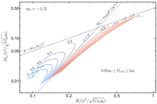
Figure 1: Phase diagram showing the effective gravitational mass ($M_{g}$) and radius ($R$) of a spherical object, with uniform ordinary-matter density $\rho_{0}$, in hydrostatic equilibrium, for $w_{0}=-1/3$. Each solid curve represents equilibrium configurations for values of ordinary-matter central pressure in the range $0.05\rho_{0}<P_{(c)0}<5\rho_{0}$, for a given value of $\sigma$ (indicated next to the corresponding curve). As expected, no equilibrium configuration is possible beyond the Schwarzschild limit ($R=2G_{N}M_{g}/c^{2}$; dashed line). The dot-dashed line gives the ordinary mass contained in an object with radius $R$ and uniform energy density $\rho_{0}$ — which coincides with the gravitational mass an object with the same density and radius would have (if possible) in standard GR.

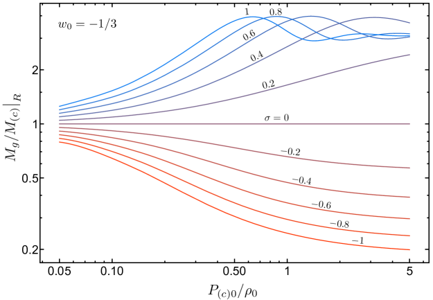
Figure 2: Ratio between the effective gravitational mass $M_{g}$ of a central body with uniform ordinary-matter density $\rho_{0}$, in case $w_{0}=-1/3$, and its ordinary mass $M_{(c)}=4\pi\rho_{0}R^{3}/(3c^{2})$ — the latter also being the gravitational mass a body with same $\rho_{0}$ and same radius $R$ would have (if possible) in standard GR. Each curve represents a given value of $\sigma$ (indicated next to the corresponding curve).

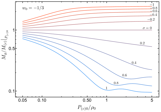
Figure 3: Ratio between the effective gravitational mass $M_{g}$ of a central body with uniform ordinary-matter density $\rho_{0}$, in case $w_{0}=-1/3$, and the ordinary mass $M_{(c)}=4\pi\rho_{0}R^{3}/(3c^{2})$ a body with same $\rho_{0}$ and same central pressure $P_{(c)0}$ would have in standard GR. Each curve represents a given value of $\sigma$ (indicated next to the corresponding curve).

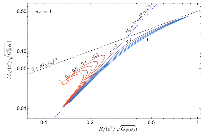
Figure 4: Phase diagram showing the effective gravitational mass ($M_{g}$) and radius ($R$) of a spherical object, with uniform ordinary-matter density $\rho_{0}$, in hydrostatic equilibrium, for $w_{0}=1$. Each solid curve represents equilibrium configurations for varying ordinary-matter central pressures ($P_{(c)0}$), for a given value of $\sigma$ (indicated next to the corresponding curve, when possible; the curves in between the ones with $\sigma=0.2$ and $\sigma=1$ correspond to $\sigma=0.4$, $0.6$, and $0.8$, in this order). As expected, no equilibrium configuration is possible beyond the Schwarzschild limit ($R=2G_{N}M_{g}/c^{2}$; dashed line). The dot-dashed line gives the ordinary mass contained in an object with radius $R$ and uniform energy density $\rho_{0}$ — which coincides with the gravitational mass an object with the same density and radius would have (if possible) in standard GR.

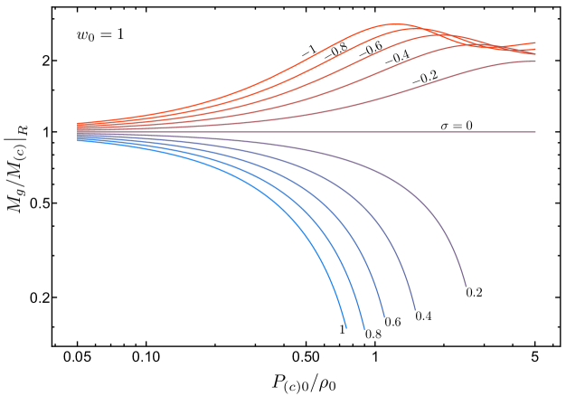
Figure 5: Ratio between the effective gravitational mass $M_{g}$ of a central body with uniform ordinary-matter density $\rho_{0}$, in case $w_{0}=1$, and its ordinary mass $M_{(c)}=4\pi\rho_{0}R^{3}/(3c^{2})$ — the latter also being the gravitational mass a body with same $\rho_{0}$ and same radius $R$ would have (if possible) in standard GR. Each curve represents a given value of $\sigma$ (indicated next to the corresponding curve).

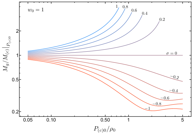
Figure 6: Ratio between the effective gravitational mass $M_{g}$ of a central body with uniform ordinary-matter density $\rho_{0}$, in case $w_{0}=1$, and the ordinary mass $M_{(c)}=4\pi\rho_{0}R^{3}/(3c^{2})$ a body with same $\rho_{0}$ and same central pressure $P_{(c)0}$ would have in standard GR. Each curve represents a given value of $\sigma$ (indicated next to the corresponding curve).

(ii) $\rho_{(nc)}=-\sigma\rho_{(c)}=-\sigma\rho_{0}$: Repeating the procedure described in the previous scenario, but now for $\rho_{(nc)}=-\sigma\rho_{(c)}=-\sigma\rho_{0}$ throughout the central object, we obtain that $P_{(nc)}$ satisfies

$$(1-\sigma)\frac{dP_{(nc)}}{dr}-(1-4\sigma)\frac{P_{(nc)}}{(\rho_{0}+P_{(c)})}\frac{dP_{(c)}}{dr}=-\frac{[4\sigma(1-\sigma)\rho_{0}+3\sigma P_{(c)}]}{(\rho_{0}+P_{(c)})}\frac{dP_{(c)}}{dr},$$ (42)

whose solution subject to the boundary condition $\left.P_{(nc)}\right|_{R}=-\left.\rho_{(nc)}\right|_{R}=\sigma\rho_{0}$ reads (for $\sigma\neq 1$ )

$$P_{(nc)}=\sigma\rho_{0}-(\rho_{0}+P_{(c)})\left[1-\left(1+\frac{P_{(c)}}{\rho_{0}}\right)^{\!\!-\frac{3\sigma}{1-\sigma}}\right].$$ (43)

Feeding this relation into Eqs. (27) and (28) determines $\rho_{\text{\it eff}}$ and $P_{\text{\it eff}}$ explicitly in terms of $P_{(c)}$, closing, again, the system of Eqs. (34)-(37) for $g$, $\phi$, $P_{(c)}$, and $m_{\text{\it eff}}$. In Figs. 7-9 we plot the same quantities as for the previous scenario (except for the omission of the uninteresting case $\sigma=1$). Notice that the effect of different values of $\sigma$ in the present scenario exhibits some similarities with the case $w_{0}>1/3$ of the previous scenario.

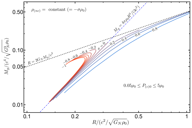
Figure 7: Phase diagram showing the effective gravitational mass ($M_{g}$) and radius ($R$) of a spherical object with uniform energy densities $\rho_{(c)}=\rho_{0}$ and $\rho_{(nc)}=-\sigma\rho_{0}$, in hydrostatic equilibrium. Each solid curve represents equilibrium configurations for values of ordinary-matter central pressure in the range $0.05\rho_{0}<P_{(c)0}<5\rho_{0}$, for a given value of $\sigma$ (indicated next to the corresponding curve). As expected, no equilibrium configuration is possible beyond the Schwarzschild limit ($R=2G_{N}M_{g}/c^{2}$; dashed line). The dot-dashed line gives the ordinary mass contained in an object with radius $R$ and uniform energy density $\rho_{0}$ — which coincides with the gravitational mass an object with the same density and radius would have (if possible) in standard GR.

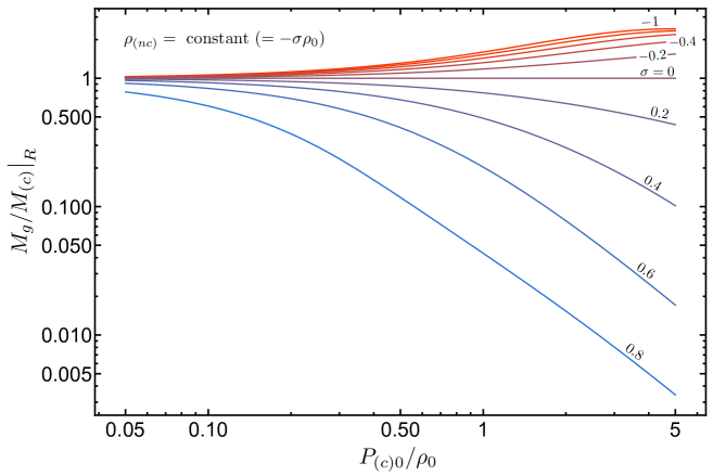
Figure 8: Ratio between the effective gravitational mass $M_{g}$ of a central body with uniform energy densities ($\rho_{(c)}=\rho_{0}$, $\rho_{(nc)}=-\sigma\rho_{0}$) and its ordinary mass $M_{(c)}=4\pi\rho_{0}R^{3}/(3c^{2})$ — the latter also being the gravitational mass a body with same $\rho_{0}$ and same radius $R$ would have (if possible) in standard GR. Each curve represents a given value of $\sigma$ (indicated next to the corresponding curve, when possible; the curves in between the ones with $\sigma=-0.4$ and $\sigma=-1$ correspond to $\sigma=-0.6$ and $-0.8$, in this order).

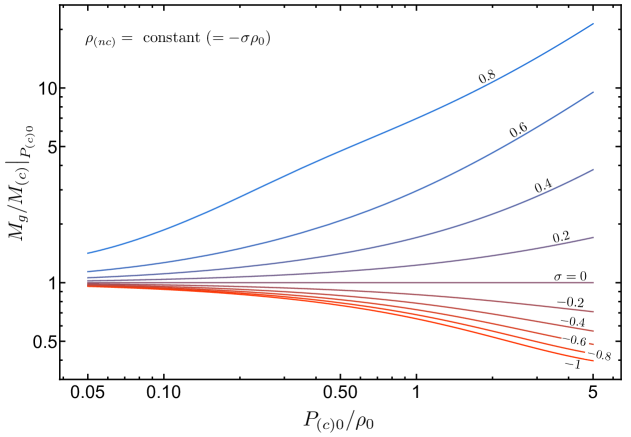
Figure 9: Ratio between the effective gravitational mass $M_{g}$ of a central body with uniform energy densities ($\rho_{(c)}=\rho_{0}$, $\rho_{(nc)}=-\sigma\rho_{0}$) and the ordinary mass $M_{(c)}=4\pi\rho_{0}R^{3}/(3c^{2})$ a body with same $\rho_{0}$ and same central pressure $P_{(c)0}$ would have in standard GR. Each curve represents a given value of $\sigma$ (indicated next to the corresponding curve).

VIII Modified cosmology

Now, we proceed to investigate possible consequences of Eq. (25) to spatially homogeneous and isotropic cosmology. Considering the FLRW line element

$$ds^{2}=-c^{2}dt^{2}+a(t)^{2}d\Sigma_{(k)}^{2},$$

with $d\Sigma_{(k)}^{2}$ being the Riemannian line element of a unit 3-sphere ($k=1$), an Euclidean 3-space ($k=0$) or a unit hyperbolic 3-space ($k=-1$) and $a(t)$ being the scale factor, Eq. (25) implies the usual Friedmann equations for the effective energy density and pressure [see Eqs. (27) and (28)]:

$$\left(\frac{\dot{a}}{a}\right)^{\!\!2}\!\! = \frac{8\pi G_{N}}{3c^{2}}\rho_{\text{\it eff}}-\frac{kc^{2}}{a^{2}},$$ (44)

$$\frac{\ddot{a}}{a} = -\frac{4\pi G_{N}}{3c^{2}}(\rho_{\text{\it eff}}-3P_{\text{\it eff}}),$$ (45)

where each dot represents derivative w.r.t. $t$. Moreover, Eq. (3) applied to each constituent ${\cal U}_{j}$ (with no nongravitational interactions) reads

$$\frac{d\rho_{j}}{dt}+3\frac{\dot{a}}{a}(\rho_{j}+P_{j})=-\sigma_{j}\frac{d}{dt}(\rho_{\text{\it eff}}-3P_{\text{\it eff}}),$$ (46)

which summed over $j$ leads to

$$\frac{d\rho_{\text{\it eff}}}{dt}+3\frac{\dot{a}}{a}(\rho_{\text{\it eff}}+P_{\text{\it eff}})=0$$ (47)

— the latter also being a direct consequence of Eqs. (44) and (45). In terms of ${\cal U}_{(c)}$ and ${\cal U}_{(nc)}$, these equations imply

$$\frac{d}{dt}\left[\rho_{(nc)}-3\bar{\sigma}(\rho_{(nc)}+P_{(nc)})\right]+3(1-4\bar{\sigma})\frac{\dot{a}}{a}(\rho_{(nc)}+P_{(nc)})=-\bar{\sigma}\frac{d}{dt}(\rho_{(c)}-3P_{(c)}).$$ (48)

It is interesting to note that out of the usual ingredients considered in cosmological scenarios — namely, radiation, whose energy density and pressure are, respectively, $\rho_{r}=\rho_{r0}(a_{0}/a)^{4}$ and $P_{r}=\rho_{r}/3$, and nonrelativistic matter (“dust”), whose energy density and pressure are $\rho_{m}=\rho_{m0}(a_{0}/a)^{3}$ and $P_{m}=0$ (subscript “0” indicates present value of the corresponding quantity) —, only nonrelativistic matter contributes to the r.h.s. of Eq. (48).

Assuming, for simplicity, that ${\cal U}_{(nc)}$ is characterized by a constant equation of state $w_{(nc)}:=P_{(nc)}/\rho_{(nc)}$ and using $\rho_{(c)}=\rho_{m}+\rho_{r}$ and $P_{(c)}=P_{r}+P_{m}$, Eq. (48) can be integrated to give

$$\rho_{(nc)}=\frac{\bar{\sigma}\rho_{m}}{[w_{(nc)}-\bar{\sigma}(1+w_{(nc)})]}+Ca^{-\frac{3(1-4\bar{\sigma})(1+w_{(nc)})}{[1-3\bar{\sigma}(1+w_{(nc)})]}},$$ (49)

where $C$ is a mere integration constant. Substituting this result into the expression for $\rho_{\text{\it eff}}$ — which is the relevant quantity to determine the expansion rate of the universe [see Eq. (44)] — and $P_{\text{\it eff}}$ — which influences the acceleration of the expansion [see Eq. (45)] —, we have

$$\rho_{\text{\it eff}} = \frac{w_{(nc)}\rho_{m}}{\alpha[w_{(nc)}-\bar{\sigma}(1+w_{(nc)})]}+\frac{\rho_{r}}{\alpha}+\frac{[1-3\bar{\sigma}(1+w_{(nc)})]}{\alpha(1-4\bar{\sigma})}Ca^{-\frac{3(1-4\bar{\sigma})(1+w_{(nc)})}{[1-3\bar{\sigma}(1+w_{(nc)})]}},$$ (50)

$$P_{\text{\it eff}} = \frac{\rho_{r}}{3\alpha}+\frac{[w_{(nc)}-\bar{\sigma}(1+w_{(nc)})]}{\alpha(1-4\bar{\sigma})}Ca^{-\frac{3(1-4\bar{\sigma})(1+w_{(nc)})}{[1-3\bar{\sigma}(1+w_{(nc)})]}}.$$ (51)

Now, we must proceed with some caution. The reader might be ready to identify $w_{(nc)}\equiv w_{0}$ and use Eq. (23), which would then lead to

$$\rho_{\text{\it eff}} = \rho_{m}+\frac{\rho_{r}}{1+\sigma(1+w_{0}^{-1})}+\frac{[1+\sigma(1+w_{0})(w_{0}^{-1}-3)]}{[1+\sigma(1+w_{0}^{-1})][1+\sigma(w_{0}^{-1}-3)]}Ca^{-\frac{3(1+w_{0})[1+\sigma(w_{0}^{-1}-3)]}{[1+\sigma(1+w_{0})(w_{0}^{-1}-3)]}},$$ (52)

$$P_{\text{\it eff}} = \frac{\rho_{r}}{3[1+\sigma(1+w_{0}^{-1})]}+\frac{w_{0}}{[1+\sigma(1+w_{0}^{-1})][1+\sigma(w_{0}^{-1}-3)]}Ca^{-\frac{3(1+w_{0})[1+\sigma(w_{0}^{-1}-3)]}{[1+\sigma(1+w_{0})(w_{0}^{-1}-3)]}}.$$ (53)

And this indeed makes sense in case ${\cal U}_{(nc)}$ has a single component with a fixed equation of state — as considered in scenario (i) of the previous section. However, in case $\rho_{(nc)}$ and $P_{(nc)}$ can be sourced independently — as in scenario (ii) of the previous section —, $w_{(nc)}$ and $w_{0}$ do not have to match. In fact, notice that $w_{0}$, referring to the static, spatially inhomogeneous energy distribution in the Newtonian regime, cannot vanish, while in the spatially homogeneous scenario nothing forbids $P_{(nc)}$ (and, therefore, $w_{(nc)}$) to be null. In particular, a simple cosmological analogous of scenario (ii) of the previous section would be one with $w_{0}=-1$ (see Sec. V) and $w_{(nc)}=0$ (a dust-like homogeneous dark constituent), leading to

$$\rho_{\text{\it eff}}=\rho_{r}+\frac{(1-3\sigma)}{(1-4\sigma)}Ca^{-\frac{3(1-4\sigma)}{(1-3\sigma)}},$$ (54)

$$P_{\text{\it eff}}=\frac{\rho_{r}}{3}-\frac{\sigma}{(1-4\sigma)}Ca^{-\frac{3(1-4\sigma)}{(1-3\sigma)}}.$$ (55)

The most interesting aspect of the results presented in Eqs. (50)-(55) is that a nonconservative constituent ${\cal U}_{(nc)}$ with given equation of state $w_{(nc)}$ can mimic a conservative ingredient with an effective equation of state

$$w_{\text{\it eff}}=\frac{w_{(nc)}-\bar{\sigma}(1+w_{(nc)})}{1-3\bar{\sigma}(1+w_{(nc)})}$$ (56)

when the data are interpreted through the lens of standard GR. In particular, if we consider $w_{(nc)}=w_{0}$ [as in Eqs. (52) and (53)], we have

$$w_{\text{\it eff}}=\frac{w_{0}}{1+{\sigma}(1+w_{0})(w_{0}^{-1}-3)}.$$ (57)

Moreover, in the scenario where $w_{(nc)}$ and $w_{0}$ are independent, there is also a residual effect of the nonconservative equations on the conservative constituents ${\cal U}_{(c)}$: interpreted through the lens of standard GR, the effective amount of nonrelativistic matter and radiation relate to the actual values by the multiplicative factors $\alpha^{-1}w_{(nc)}/[w_{(nc)}-\bar{\sigma}(1+w_{(nc)})]$ and $\alpha^{-1}$, respectively [see Eq. (50)]. All these results combined open up the possibility of a “dark” ingredient ${\cal U}_{(nc)}$ being responsible, at once, for driving the cosmic expansion through an accelerating phase (if $w_{\text{\it eff}}<-1/3$, $\rho_{\text{\it eff}}>0$) and for an excess in the (gravitationally) observed amount of nonrelativistic matter (if $\alpha^{-1}w_{(nc)}/[w_{(nc)}-\bar{\sigma}(1+w_{(nc)})]>1$).

Using Eqs. (56) and (57), in Figs. 10 and 11 we highlight the regions in the parameter spaces $\{(w_{(nc)},\bar{\sigma})\}$ and $\{(w_{0},{\sigma})\}$, respectively, where $w_{\text{\it eff}}<-1/3$ — which represent models with late accelerating cosmic expansion (for $\rho_{\text{\it eff}}>0$). We also represent curves where $w_{\text{\it eff}}$ assumes some constant values (given next to the corresponding curve). This is only to make it clearer that in the scenario where $w_{(nc)}$ and $w_{0}$ are independent (Fig. 10), even a dust-like nonconservative constituent ($w_{(nc)}=0$) could, in principle, mimic a dark-energy-like ingredient in standard GR.

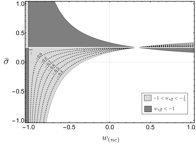
Figure 10: Diagram showing the values $(w_{(nc)},\bar{\sigma})$ for which $-1<w_{\text{\it eff}}<-1/3$ (light-gray region) and $w_{\text{\it eff}}<-1$ (dark-gray region) — according to Eq. (56). The dashed curves represent constant values of $w_{\text{\it eff}}$ (given next to the corresponding curve).

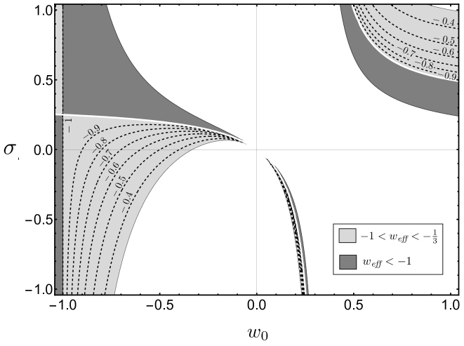
Figure 11: Diagram showing the values $(w_{0},{\sigma})$ for which $-1<w_{\text{\it eff}}<-1/3$ (light-gray region) and $w_{\text{\it eff}}<-1$ (dark-gray region) — according to Eq. (57). The dashed curves represent constant values of $w_{\text{\it eff}}$ (given next to the corresponding curve).

IX Conclusion

In the present work, we have investigated to which extent the canon of local energy-momentum conservation applied to matter/interaction fields (other than gravity) — as enforced by standard GR and other metric theories of gravity through Eq. (1) with $\nabla_{a}{\cal G}^{ab}\equiv 0$ — can be challenged to allow local energy-momentum exchange between the nongravitational system and the spacetime. There are several ways in which such an exchange of energy-momentum can take place without violating the other (seemingly more natural) canon of general covariance. As a proof of concept and in the absence of a fundamental description of how such an exchange could occur, here we adopted a phenomenological approach and explored the simplest model one could devise, given by Eqs. (2) and (3) — which generalizes the model proposed by Rastall fifty years ago Rastall , explored in subsequent works LH ; BDFPR ; OVFC ; OVF ; Visser . Although the distinction between Rastall’s theory — Eq. (2) with an ingredient-independent parameter $\sigma$ — and our Rastall-like model — Eq. (3) with ingredient-dependent parameters $\sigma_{j}$ — might seem unimportant at first, we have explicitly shown that it is enough, in a universe containing “dark” ingredients (such as ours), to render the latter immune to the criticisms which are used to discard the former as a viable model. Interestingly enough, in spite of our primary motivation relying purely on “naturality” arguments, we showed that this issue of “nonconservative gravity” gets tied to the existence of “dark” ingredients in our Universe — a connection which seems to have been overlooked in the literature. This fact is essential when confronting the consequences of the model with observations and it bears effects on many of the results presented in this manuscript (summarized in Figs. 1-11). In fact, were we living in a Universe with no room for “dark” ingredients and the Rastall-like model given by Eq. (3) (with $T^{ab}_{(j)}$ being the physical stress-energy-momentum tensor) would have been discarded (or at least have the $\sigma_{j}$ parameters severely constrained) by simple observations of lower bounds on pressure-density ratios in the Newtonian regime (Sec. IV). On the other hand, as we have discussed in Sec. VIII, a “dark” nonconservative ingredient satisfying Eq. (3) could, in principle, mimic dark-energy and dark-matter effects, at once, when observations are interpreted through the lens of standard GR. Hence, although a violation of $\nabla_{a}T^{ab}=0$ may seem “radical” at first, analyses like the one presented here suggest otherwise: not only it is natural (from a logical perspective), but it also finds room to be true in our observed Universe.

References

- (1) H. Velten and T. Caramês. To Conserve, or Not to Conserve: A Review of Nonconservative Theories of Gravity, Universe 7, 38 (2021).
- (2) T. Harko, F. S. N. Lobo, S. Nojiri, and S. D. Odintsov. gravity, Phys. Rev. D 84, 024020 (2011).
- (3) P. Rastall. Generalization of the Einstein theory, Phys. Rev. D 6, 3357 (1972).
- (4) L. Lindblom and W. A. Hiscock. Criticism of some non-conservative gravitational theories, J. Phys. A 15, 1827-1830 (1982).
- (5) C. E. M. Batista, M. H. Daouda, J. C. Fabris, O. F. Piattella, and D. C. Rodrigues. Rastall cosmology and the CDM model, Phys. Rev. D 85, 084008 (2012).
- (6) A. M. Oliveira, H. E. S. Velten, J. C. Fabris, and L. Casarini. Neutron stars in Rastall gravity, Phys. Rev. D 92, 044020 (2015).
- (7) A. M. Oliveira, H. E. S. Velten, and J. C. Fabris. Nontrivial static, spherically symmetric vacuum solution in a nonconservative theory of gravity, Phys. Rev. D 93, 124020 (2016).
- (8) M. Visser. Rastall gravity is equivalent to Einstein gravity, Phys. Lett. B 782, 83-86 (2018).