Continuously varying critical exponents in long-range quantum spin ladders

Abstract

We investigate the quantum-critical behavior between the rung-singlet phase with hidden string order and the Néel phase with broken $SU(2)$-symmetry on quantum spin ladders with algebraically decaying unfrustrated long-range Heisenberg interactions. Combining perturbative continuous unitary transformations (pCUT) with a white-graph expansion and Monte Carlo simulations yields high-order series expansions of energies and observables in the thermodynamic limit about the isolated rung-dimer limit. The breakdown of the rung-singlet phase allows to determine the critical line and the entire set of critical exponents as a function of the decay exponent of the long-range interaction. A non-trivial regime of continuously varying critical exponents as well as long-range mean-field behavior is demonstrated reminiscent of the long-range transverse-field Ising model.

Introduction.- While in electromagnetism the interaction between charged particles is long-range decaying as a power-law with distance, in condensed matter systems the interaction is typically screened, justifying to consider short-range interactions in most microscopic investigations. There are, however, notable examples where the long-range behavior persists like in conventional dipolar ferromagnetism Bitko et al. (1996); Chakraborty et al. (2004) and exotic spin-ice materials Bramwell and Gingras (2001); Castelnovo et al. (2008) giving rise to magnetic monopoles. In quantum optical platforms, long-range interactions are commonly present and there has been formidable experimental advancements over the past decades. Indeed, among others, ions in magneto-optical traps Islam et al. (2011); Britton et al. (2012); Islam et al. (2013); Jurcevic et al. (2014); Richerme et al. (2014); Mielenz et al. (2016); Bohnet et al. (2016); Jurcevic et al. (2017); Zhang et al. (2017); Žunkovič et al. (2018); Hempel et al. (2018); Joshi et al. (2022) and neutral atoms in optical lattices Weimer et al. (2010); Xia et al. (2015); Labuhn et al. (2016); Wang et al. (2016); Schauss (2018); de Léséleuc et al. (2019); Levine et al. (2019); Wu et al. (2019); Ebadi et al. (2021); Semeghini et al. (2021) have gained vast attention as these platforms can realize one- and two-dimensional lattices with adaptable geometries and a mesoscopic number of entities offering high-fidelity control and read-out. This makes them viable candidates for versatile quantum simulators and scalable quantum computers Saffman et al. (2010); Bruzewicz et al. (2019); Browaeys and Lahaye (2020). Both platforms realize effective Ising- and XY-type spin interactions which decay algebraically with distance. In neutral-atom platforms the decay exponent is fixed while it can be continuously tuned in trapped-ion systems. Recent progress ranges from the determination of molecular ground-state energies Hempel et al. (2018) and the realization of equilibrium Islam et al. (2011); Ebadi et al. (2021) and dynamical quantum phase transitions Zhang et al. (2017); Jurcevic et al. (2017); Žunkovič et al. (2018) to the direct observation of a symmetry-protected topological phase de Léséleuc et al. (2019) or a topologically-ordered quantum spin liquid Semeghini et al. (2021) by measuring non-local string operators.
The majority of numerical studies has focused on a variety of spin chains Sandvik (2003); Koffel et al. (2012); Knap et al. (2013); Sun (2017); Zhu et al. (2018); Sandvik (2010); Vanderstraeten et al. (2018); Fey and Schmidt (2016); Adelhardt et al. (2020); Langheld et al. (2022); Yang et al. (2020a); Yusuf et al. (2004); Laflorencie et al. (2005); Zhu and Wang (2006); Li and Wang (2015); Tang and Sandvik (2015); Gong et al. (2016); Maghrebi et al. (2017); Ren et al. (2020); Yang et al. (2020a); Vodola et al. (2014, 2015); Gong et al. (2016); Maity et al. (2019); Sadhukhan and Dziarmaga (2021) as well as two-dimensional systems directly related to Rydberg atom platforms with quickly decaying ($\sim r^{-6}$) long-range interactions Samajdar et al. (2021); Verresen et al. (2021); Liu et al. (2022). One prominent exception is the long-range transverse-field Ising model (LRTFIM), which was recently analyzed on the two-dimensional square and triangular lattice with tunable long-range interactions Humeniuk (2016); Fey et al. (2019); Koziol et al. (2021). Geometrically unfrustrated LRTFIMs in one and two dimensions are known to display three distinct regimes of quantum criticality between the high-field polarized phase and the low-field $\mathbb{Z}_{2}$-symmetry broken ground state: For short-range interactions the system exhibits nearest-neighbor criticality, for strong long-range interactions long-range mean-field behavior, and in-between continuously varying critical exponents Dutta and Bhattacharjee (2001); Sak (1973); Defenu et al. (2017); Behan et al. (2017a, b); Defenu et al. (2020).
Less is known about the quantum-critical behavior of systems with long-range interactions possessing a continuous symmetry like the antiferromagnetic spin-1/2 Heisenberg model. For the one-dimensional short-range Heisenberg chain, the spontaneous breaking of its continuous $SU(2)$-symmetry is forbidden by the Mermin-Wagner theorem Mermin and Wagner (1966); Hohenberg (1967); Coleman (1973); Bruno (2001) and the system displays quasi long-range order with gapless fractional spinon excitations. Interestingly, this theorem can be circumvented when unfrustrated long-range interactions are sufficiently strong giving rise to a quantum phase transition to a Néel state with broken $SU(2)$-symmetry Yusuf et al. (2004); Laflorencie et al. (2005); Sandvik (2010); Tang and Sandvik (2015); Maghrebi et al. (2017); Yang et al. (2020a); Yang and Feiguin (2021). Furthermore, a recent work Yang et al. (2020b) has studied antiferromagnetic two-leg quantum spin ladders with unfrustrated long-range Heisenberg interactions. Here a quantum phase transition between the gapped short-range isotropic ladder and the Néel state with broken $SU(2)$-symmetry is present. Since the isotropic ladder displays a rung-singlet phase with non-local string-order parameter, a deconfined criticality Vishwanath et al. (2004); Senthil et al. (2004a, b, 2005) between two distinct ordered quantum phases has been suggested.
In this letter, we investigate two types of long-range quantum spin ladders with arbitrary ratios of nearest-neighbor leg and rung exchange coupling and for arbitrary decay exponent of the long-range Heisenberg interaction so that the system studied in Ref. Yang et al. (2020b) is contained as one specific parameter line. To this end we extend the pCUT approach developed in Ref. Fey et al. (2019) to generic observables which allows us to locate the critical breakdown of the rung-singlet phase and determine the entire set of canonical critical exponents as a function of the decay exponent. A non-trivial regime of continuously varying critical exponents as well as long-range mean-field behavior is observed similar to the LRTFIM implying the absence of deconfined criticality.

Model.- We consider the following spin-$1/2$ Hamiltonian

$$\begin{split}\mathcal{H}=J_{\perp}&\sum_{i}\vec{S}_{i,1}\vec{S}_{i,2}-\sum_{i,\delta>0}\sum_{n=1}^{2}J_{\shortparallel}(\delta)\vec{S}_{i,n}\vec{S}_{i+\delta,n}\\ &-\sum_{i,\delta>0}J_{\times}(\delta)\left(\vec{S}_{i,1}\vec{S}_{i+\delta,2}+\vec{S}_{i,2}\vec{S}_{i+\delta,1}\right),\end{split}$$ (1)

where the indices $i$ and $i+\delta$ denote the rung position, the second index $n\in\{1,2\}$ the leg of the ladder and the exchange parameters $J_{\perp}>0$, $J_{\shortparallel}(\delta)$, and $J_{\times}(\delta)$ couple spin operators on the rungs, legs, and diagonals, respectively. In the following, we restrict to the limiting cases $\mathcal{H}_{\shortparallel}\equiv\mathcal{H}|_{J_{\times}=0}$ and $\mathcal{H}_{\bowtie}\equiv\mathcal{H}|_{J_{\shortparallel}=J_{\times}}$, set $J_{\perp}=1$, and introduce $\lambda=J$ with $J\equiv J_{\shortparallel}$. Further, we define the distant-dependent coupling parameters to be of the form

$$\begin{gathered}\begin{aligned} &\lambda_{\shortparallel}(\delta)=\lambda\frac{(-1)^{\delta}}{|\delta|^{1+\sigma}},\quad&\lambda_{\times}(\delta)=\lambda\frac{(-1)^{1+\delta}}{|1+\delta|^{1+\sigma}},\end{aligned}\end{gathered}$$ (2)

with $\lambda\geq 0$ realizing an unfrustrated algebraically decaying long-range interaction which induces antiferromagnetic Néel ordering for sufficiently small $\sigma$. Indeed, the decay exponent $\sigma$ can be tuned between the limiting cases of all-to-all interactions at $\sigma=-1$ and nearest-rung couplings at $\sigma=\infty$ (see Fig. 1 for an illustration of the two different ladder models $\mathcal{H}_{\shortparallel}$ and $\mathcal{H}_{\bowtie}$ in the neighboring rung limit). Here, we focus on $\sigma\geq 0$ so that the energy of the system is extensive in the thermodynamic limit.

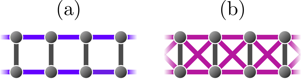
Figure 1: Illustration of the two underlying short-range quantum spin ladders with nearest-neighbor Heisenberg interaction $J_{\perp}$ on rung dimers as well as Heisenberg couplings between nearest-neighbor rung dimers (a) along the legs $\mathcal{H}_{\shortparallel}$ or (b) along the legs and the diagonals $\mathcal{H}_{\bowtie}$.

In the limit of isolated rung dimers $\lambda=0$, the ground state is given exactly by the product state of rung singlets $\ket{s}=\leavevmode\nobreak\ \left(\ket{\uparrow\downarrow}-\ket{\downarrow\uparrow}\right)/\sqrt{2}$ with localized rung triplets $\ket{t_{x}}=-(\ket{\uparrow\uparrow}-\ket{\downarrow\downarrow})/\sqrt{2}$, $\ket{t_{y}}={\rm i}(\ket{\uparrow\uparrow}+\ket{\downarrow\downarrow})/\sqrt{2}$, and $\ket{t_{z}}=\left(\ket{\uparrow\downarrow}+\ket{\downarrow\uparrow}\right)/\sqrt{2}$ as elementary excitations. For small $\lambda$ the ground state is adiabatically connected to this product state and the system is in the rung-singlet phase. The associated elementary excitations of the rung-singlet phase are gapped triplons corresponding to dressed rung-triplet excitations. For $\mathcal{H}_{\shortparallel}$ and $\sigma=\infty$ this holds for any finite $\lambda$ and only at $\lambda=\infty$ the system decouples into two spin-1/2 Heisenberg chains with gapless spinon excitations and a quasi long-range ordered ground state. In contrast, the Hamiltonian $\mathcal{H}_{\bowtie}$ becomes a diagonal spin-ladder at $\lambda=\infty$ for $\sigma=\infty$ and is expected to realize the gapped Haldane phase with exponentially decaying correlations for $\lambda>2$ falling into the category of symmetry-protected topological phases Kim et al. (2000); Pollmann et al. (2012). The ground states of both Heisenberg ladders at any finite $\lambda$ only break a hidden $\mathbb{Z}_{2}\times\mathbb{Z}_{2}$ symmetry and can be characterized by non-local string order parameters Takada and Watanabe (1992); Watanabe (1995); Nishiyama et al. (1995); White (1996); Kim et al. (2000).
Previous studies of the spin-$1/2$ Heisenberg chain Yusuf et al. (2004); Laflorencie et al. (2005); Tang and Sandvik (2015); Yang et al. (2020a) and the two-leg ladder $\mathcal{H}_{\bowtie}$ for $\lambda=1$ Yang et al. (2020b) with unfrustrated long-range interactions deduced a quantum phase transition towards Néel order with broken $SU(2)$-symmetry and thus circumventing the Mermin-Wagner theorem Mermin and Wagner (1966); Hohenberg (1967); Coleman (1973). Further, Goldstone’s theorem states that the spontaneous breaking of a continuous symmetry gives rise to massless Nambu-Goldstone modes Nambu (1960); Goldstone (1961); Goldstone et al. (1962), however, the same restriction applies and the theorem loses its validity in the presence of long-range interactions. Indeed, in the extreme case of an all-to-all coupling the elementary excitation above the superextensive ground-state energy becomes proportional to the system size, evidently breaking Goldstone’s theorem Yusuf et al. (2004); Yang et al. (2020b).

pCUT method.- Interpreting the Heisenberg ladders as systems of coupled dimers, we introduce hard-core bosonic triplet (creation) annihilation operators $t_{i,\rho}^{(\dagger)}$ (creating) annihilating local triplets with flavor $\rho\in\{x,y,z\}$ on rung $i$ Sachdev and Bhatt (1990); Hörmann et al. (2018), the Hamiltonian (1) can be written as

$$\mathcal{H}=\mathcal{H}_{0}+\mathcal{V}=E_{0}+\mathcal{Q}+\sum_{\delta>0}\lambda(\delta)\sum_{m=-2}^{2}T_{m},$$ (3)

where the unperturbed Hamiltonian of decoupled rungs is $\mathcal{H}_{0}=E_{0}+\mathcal{Q}$ and $E_{0}=-3/4N_{\rm rung}$ is the unperturbed ground-state energy with $N_{\rm rung}$ the number of rungs, $\mathcal{Q}=\sum_{i,\rho}t_{i,\rho}^{\dagger}t_{i,\rho}^{\phantom{\dagger}}$ counts the number of triplet quasi-particles (QPs), and the perturbation $\mathcal{V}$ decomposes into a sum of operators $T_{m}$ containing processes of triplet operators that change the system’s energy by $m\in\{0,\pm 2\}$ quanta. In the following we employ high-order series expansions along the same lines as in previous studies on the LRTFIM Fey et al. (2019); Koziol et al. (2019); Adelhardt et al. (2020); Langheld et al. (2022). The pCUT method Knetter and Uhrig (2000); Knetter et al. (2003) transforms the original Hamiltonian $\mathcal{H}$, perturbatively order by order in $\lambda$, into an effective Hamiltonian $\mathcal{H}_{\text{eff}}$ which conserves the number of triplon excitations $[\mathcal{Q},\mathcal{H}_{\text{eff}}]=0$. Similarly, observables $\mathcal{O}$ can be mapped to effective observables $\mathcal{O}_{\text{eff}}$ resulting in an expression analogous to $\mathcal{H}_{\text{eff}}$. However, the quasiparticle-conserving property is lost Knetter et al. (2003). In a next step the effective Hamiltonian and observables have to be normal-ordered which is most efficiently done via a full-graph decomposition exploiting the linked-cluster theorem Coester and Schmidt (2015). For long-range interactions this is only feasible by applying a white-graph expansion Coester and Schmidt (2015); Fey and Schmidt (2016), i.e., the most general linked contribution of a graph is extracted. To obtain the physical properties in the thermodynamic limit these general white-graph contributions have to be embedded on an infinite chain with rung dimers as effective supersites. Due to the presence of long-range interactions, every realization of a graph on the lattice except for overlapping configurations is possible leading to infinite nested sums that are evaluated using Markov-chain Monte Carlo integration for a fixed decay exponent $\sigma$ Fey et al. (2019) (see also Ref. Sup for details).
After applying the above procedure and Fourier transforming into quasi-momentum space, the effective one-triplon (1QP) Hamiltonian reads

$$\tilde{\mathcal{H}}_{\text{eff}}^{\text{1QP}}=\bar{E}_{0}+\sum_{k,\rho}\omega(k)t^{\dagger}_{k,\rho}t_{k,\rho}^{\phantom{\dagger}},$$ (4)

with the ground-state energy $\bar{E}_{0}$ and the 1QP dispersion $\omega(k)$. We can calculate the control-parameter susceptibility and the elementary one-triplon excitation gap directly

$$\begin{gathered}\begin{aligned} &\chi=\derivative[2]{\bar{E}_{0}}{\lambda},\qquad&\Delta=\min_{k}\omega(k)=\omega(k_{\rm c})\end{aligned}\end{gathered}$$ (5)

with the critical momentum $k_{\rm c}=\pi$ for antiferromagnetic interactions. We further determine the one-triplon spectral weight. With $\mathcal{O}_{\rho}(k)=\frac{1}{2}(t_{k,\rho}^{\dagger}+t_{k,\rho}^{\phantom{\dagger}})$, one finds

$$\mathcal{S}^{\rm 1QP}(k)=\left|\bra{t_{k,\rho}}\mathcal{O}^{\text{1QP}}_{\text{eff},\rho}(k)\ket{\rm ref}\right|^{2}=|s(k)|^{2},$$ (6)

where $\ket{\text{ref}}=\bigotimes_{i}\ket{s_{i}}$ is the unperturbed rung-singlet ground state, $\ket{t_{k,\rho}}$ is the one-triplon state with momentum $k$ and flavor $\rho\in\{x,y,z\}$, and $\mathcal{O}^{\text{1QP}}_{\text{eff},\rho}(k)=s(k)(t_{k,\rho}^{\dagger}+t_{k,\rho}^{\phantom{\dagger}})$ the effective observable in second quantization restricted to the one-triplon channel. Here, we calculated the perturbative series of the ground-state energy $\bar{E}_{0}$ up to order 12 (8), the elementary gap $\Delta$ up to order 10 (7), and the one-triplon spectral weight $\mathcal{S}^{\rm 1QP}(k_{c})$ up to order 9 (7) in the perturbation parameter $\lambda$ for $\mathcal{H}_{\shortparallel}$ ($\mathcal{H}_{\bowtie}$).
The above quantities show the dominant power-law behavior

$$\chi \sim|\lambda-\lambda_{\rm c}|^{-\alpha},$$ (7)

$$\Delta \sim|\lambda-\lambda_{\rm c}|^{z\nu},$$ (8)

$$\mathcal{S}^{\rm 1QP}(k_{\rm c}) \sim|\lambda-\lambda_{\rm c}|^{-(2-z-\eta)\nu}$$ (9)

close to the critical point $\lambda_{c}$ when the rung-singlet phase breaks down. The critical point and associated critical exponents can be directly determined from physical poles and associated residuals using (biased) DlogPadé extrapolants. More detailed information on the employed procedure from the graph embedding to extrapolations can be found in Ref. Sup .

Quantum phase diagram.- We determine the phase transition point $\lambda_{\rm c}$ as a function of the decay exponent $\sigma$ by the quantum-critical breakdown of the rung-singlet phase and the accompanied closing of the elementary gap. The corresponding quantum phase diagram is shown in Fig. 2 for $\mathcal{H}_{\shortparallel}$ and $\mathcal{H}_{\bowtie}$. In the limit of $\lambda=0$ the system’s ground state is given by the product of rung singlets and for $\sigma>2$ a quantum phase transition can be ruled out from one-loop RG Dutta and Bhattacharjee (2001) since the $N$-component quantum rotor model can be mapped to the low-energy physics of the Heisenberg ladder Sachdev (2011) in accordance with the Mermin-Wagner theorem.

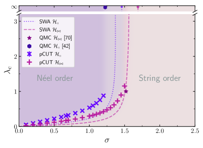
Figure 2: Phase diagram depicting the critical point $\lambda_{c}$ as a function of the decay exponent $\sigma$. Crosses are determined by DlogPadé extrapolations of the one-triplon gap series from the pCUT method while dashed lines are extracted from the self-consistency condition for the magnetization within linear spin-wave approximation (SWA). Diagonal crosses in navy blue correspond to $\mathcal{H}_{\shortparallel}$ and upright crosses in purple to $\mathcal{H}_{\bowtie}$. For the latter we observe that the Néel ordered phase sets in at smaller $\lambda$ or larger $\sigma$ exponents. The hexagon point at $\lambda=\infty$ for $\mathcal{H}_{\shortparallel}$ from Ref. Laflorencie et al. (2005) as well the star-shaped point along the $\lambda=1$ line for $\mathcal{H}_{\bowtie}$ from Ref. Yang et al. (2020b) are consistent with our results.

At small $\sigma\lesssim 0.7$ ($\sigma\lesssim 1.0$) for $\mathcal{H}_{\shortparallel}$ ($\mathcal{H}_{\bowtie}$) the critical point $\lambda_{c}$ shifts linearly towards larger $\lambda$ with increasing $\sigma$. The gap closes earlier for $\mathcal{H}_{\bowtie}$ in agreement with expectation since the additional diagonal interactions further stabilize the antiferromagnetic Néel order. For larger $\sigma$ the critical points start to deviate from the linear behavior and bend upwards towards larger critical points until eventually DlogPadé extrapolations break down when the critical point shifts away significantly from the radius of convergence of the series.
We complement the pCUT aproach with linear spin-wave calculations similar to Yusuf et al. (2004); Laflorencie et al. (2005). Exploiting the fact that spin-wave theory is expected to work in the Néel ordered phase we can to determine the quantum-critical point (see Ref. Sup ). The spin-wave results are in qualitative rather than quantitative agreement with pCUT which is no surprise considering the crude approximation. In contrast to the pCUT results, the linear spin-wave calculations can be performed up to the limit $\lambda=\infty$. We find that $\lambda_{\rm c}$ diverges inline with expectations as the absence of criticality at large enough $\sigma$ suggests the existence of an upper critical decay exponent $\sigma_{\rm c}$. In fact, for $\mathcal{H}_{\shortparallel}$ at $\lambda=\infty$ we recover the spin-wave dispersion in Ref. Laflorencie et al. (2005) yielding $\sigma^{\rm SW}_{\rm c}\approx 1.46$ and for $\mathcal{H}_{\bowtie}$ we find $\sigma^{\rm SW}_{\rm c}\approx 1.69$. Moreover, our data is consistent with $\sigma_{c}=1.225(25)$ from Ref. Laflorencie et al. (2005) for $\mathcal{H}_{\shortparallel}$ and with $\sigma\approx 1.52$ at $\lambda_{\rm c}=1$ for $\mathcal{H}_{\bowtie}$ in Ref. Yang et al. (2020b) as depicted in Fig. 2.

Critical Exponents.- We extract the critical exponents according to Eqs. (7)-(9) from DlogPadé extrapolants of the perturbative series. The exponents are depicted in Fig. 3 as a function of the decay exponent $\sigma$.

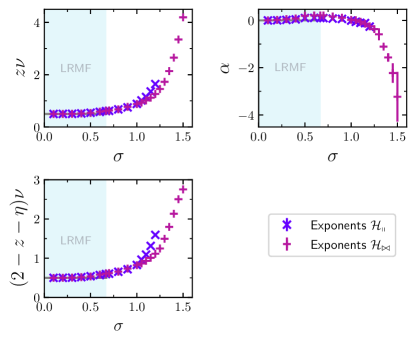
Figure 3: Critical exponents from Eqs. (7)-(9) determined by the pCUT approach as a function of the decay exponent $\sigma$ for both ladder models $\mathcal{H}_{\shortparallel}$ and $\mathcal{H}_{\bowtie}$. For $\sigma\leq 2/3$ the exponents clearly coincide with the expected long-range mean-field values (shaded region). For $\sigma>2/3$ they become continuously larger and apparently start to diverge. While the critical exponent for both models match well for $\sigma\lesssim 2.1$, they start to deviate from each other for larger values of $\sigma$ but this can probably be attributed to the difference in $\sigma_{\rm c}$.

The long-range mean-field regime (LRMF) is expected to extend to $\sigma\leq 2/3$ Dutta and Bhattacharjee (2001). The exponents extracted from DlogPadé extrapolants agree well with expected long-range mean-field exponents, although the presence of multiplicative logarithmic corrections to the dominant power-law behavior at the upper critical dimension $d_{\text{uc}}=2/(3\sigma)$ spoil the critical exponents. Excluding the $\alpha$-exponent the critical exponents deviate less than 1.1 % (1.3 %) deep in the long-range regime $\sigma\leq 0.3$ for $\mathcal{H}_{\shortparallel}$ ($\mathcal{H}_{\bowtie}$). We also observe continuously varying exponents for $\sigma>2/3$ which seem to diverge for $\sigma\rightarrow\sigma_{\rm c}$. In terms of the gap closing this can be understood from the nearest-neighbor limit where the gap does not close but with the presence of long-range interactions the finite gap is lowered until eventually the gap closes. Further strengthening the long-range interactions shifts the critical point from infinity to smaller values and thus continuously tuning the exponent $z\nu$ from infinity to smaller values as the gap closes increasingly steep. In the region $\sigma\gtrsim 2.1$ for $\mathcal{H}_{\shortparallel}$ ($\sigma\gtrsim 2.2$ for $\mathcal{H}_{\bowtie}$) close to $\sigma_{c}$ it becomes difficult to extrapolate the critical point that starts to shift quickly towards $\lambda=\infty$ and therefore negatively affects the accuracy of the exponent estimates.
Using the three critical exponents from Fig. 3, one can apply (hyper-) scaling relations to derive all canonical critical exponents (see Ref. Sup for details) which are displayed in Fig. 4 for $\mathcal{H}_{\shortparallel}$ and $\mathcal{H}_{\bowtie}$.

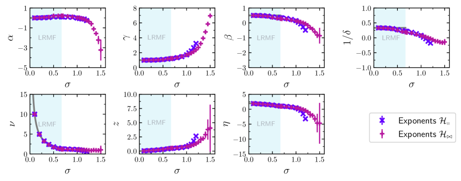
Figure 4: Canonical critical exponents obtained from (hyper-) scaling relations as a function of the decay exponent $\sigma$. The critical exponents are in good agreement with expectations in the long-range mean-field regime (shaded region) and show continuously varying exponents for $\sigma>2/3$. While some critical exponents appear to diverge others seem to go to a constant value for increasing $\sigma$. For some exponents the error bars become large for $\sigma\approx\sigma_{c}$.

In the long-range mean-field regime the exponents agree well with the expectations except for the exponents $\beta$ and $1/\delta$ around the upper critical dimension which we attribute to error propagation due to the presence of multiplicative logarithmic corrections. While the critical exponent $\gamma$ diverges for larger values of $\sigma$, the critical exponent $\nu$ approaches a constant value $\nu\approx 1$. The exponent $1/\delta$ goes to $-0.125$ in this limit, however we attribute this to a systematic error and that the correct limit might be $0$ since a jump of $\delta$ from $\infty$ to $-\infty$ is considered as unlikely. For the exponents $\beta$, $z$ and $\eta$ the uncertainty in the regime $\sigma\gtrsim 2.2$ becomes large due to error propagation and it is hard to make reliable statements in this region.
Comparing the above results with Ref. Yang et al. (2020b) for $\mathcal{H}_{\bowtie}$ at $\lambda=1$ we find that the exponent $\nu=1.8$ at about $\sigma\approx 1.5$ is inconsistent with our result with constant $\nu=0.97(7)$ for all $\sigma>1.0$. Furthermore, the monotonously increasing exponent $z>1$ for $\sigma>1.1$ is not in line with a proposed deconfined critical point with $z=1$ at $\sigma\approx 1.5$. Our finding of continuously varying exponents reminiscent of the criticality of the unfrustrated LRTFIM Dutta and Bhattacharjee (2001); Sak (1973); Defenu et al. (2017); Behan et al. (2017a, b); Defenu et al. (2020); Fey and Schmidt (2016); Fey et al. (2019) rises the question why this specific point should be extraordinary, particularly considering that despite the presence of a non-local string order parameter the rung singlet-phase of both models $\mathcal{H}_{\shortparallel}$ and $\mathcal{H}_{\bowtie}$ for all relevant $\lambda$ is not topologically protected but trivially connected to the product state of rung singlets Pollmann et al. (2012).

Conclusions.- We investigated the quantum-critical behavior of unfrustrated two-leg quantum spin ladders with long-range Heisenberg interactions by applying and extending the pCUT method using white graphs and classical Monte Carlo integration. Calculating the ground-state energy, the one-triplon gap, and the one-triplon spectral weight allows us to extract the full set of critical exponents as a function of the decay exponent by appropriate extrapolation techniques. A non-trivial regime of continuously varying critical exponents as well as long-range mean-field behavior is observed similar to the unfrustrated LRTFIM implying the absence of deconfined criticality. Let us note that our approach can be naturally extended to two-dimensional models with long-range interactions like Heisenberg bilayers offering a completely unexplored playground for future investigations.

Acknowledgments.- PA and KPS gratefully acknowledge the support by the Deutsche Forschungsgemeinschaft (DFG, German Research Foundation) – Project-ID 429529648—TRR 306 QuCoLiMa (“Quantum Cooperativity of Light and Matter”) as well as the Munich Quantum Valley, which is supported by the Bavarian state government with funds from the Hightech Agenda Bayern Plus and the scientific support and HPC resources provided by the Erlangen National High Performance Computing Center (NHR@FAU) of the Friedrich-Alexander-Universität Erlangen-Nürnberg (FAU). The hardware is funded by the DFG.

In the supplementary materials we first discuss the high-order series-expansion approach for long-range systems and extend the established approach to ground-state energies and observables. Second, we briefly introduce DlogPadé extrapolants and discuss the extrapolation scheme employed. Third, we provide the major steps of the linear spin-wave calculations used to determine the critical points within this approximations as a supplement to the pCUT results. Last, we provide an overview of scaling relations and hyperscaling which was only recently consistently generalized to the quantum long-range case Langheld et al. (2022).

I High-order series expansion

I.1 The pCUT method

In order to apply the pCUT method Knetter and Uhrig (2000); Knetter et al. (2003) it must be possible to describe the problem under consideration with a Hamiltonian of the form

$$\mathcal{H}=\mathcal{H}_{0}+\mathcal{V}=E_{0}+\mathcal{Q}+\sum_{\delta>0}^{\infty}\lambda(\delta)\mathcal{V}(\delta)\,$$ (S1)

with an unperturbed Hamiltonian $\mathcal{H}_{0}$ with equidistant spectrum that is bounded from below and a perturbation $\mathcal{V}$. The unperturbed part becomes $\mathcal{H}_{0}=E_{0}+\mathcal{Q}$ with $\mathcal{Q}=\sum_{i,\rho}t_{i,\rho}^{\dagger}t_{i,\rho}^{\phantom{\dagger}}$ counting the number of triplet quasiparticles (QPs). For long-range systems the perturbation $\mathcal{V}$ can be written as a sum between interacting processes of distance $\delta$ with a distance-dependent expansion parameter $\lambda(\delta)$. Also, the perturbation must decompose into

$$\mathcal{V}=\sum_{m=-N}^{N}\hat{T}_{m}=\sum_{m=-N}^{N}\sum_{l}\hat{\tau}_{m,l},$$ (S2)

where the operators $\hat{T}_{m}$ change the system’s energy by $m$ energy quanta such that $[\mathcal{Q},\hat{T}_{m}]=m\hat{T}_{m}$. The operator $\hat{T}_{m}$ decomposes into a sum of local operators $\hat{\tau}_{m,l}$ on a link $l$ connecting different sites of the underlying lattice. When the above prerequisites are fulfilled the pCUT method unitarily transforms the original Hamiltonian, order by order in perturbation, to an effective, quasiparticle-conserving Hamiltonian $\mathcal{H}_{\text{eff}}$ reducing the complicated many-body problem to an easier effective few-body problem. The effective Hamiltonian in a generic form for an arbitrary number of expansion parameters $\lambda_{i}$ is then given by

$$\mathcal{H}_{\text{eff}}=\mathcal{H}_{0}+\sum_{\sum_{j}n_{j}=k}^{\infty}\lambda_{1}^{n_{1}}\dots\lambda_{k}^{n_{k}}\sum_{\begin{subarray}{c}\dim(\bm{m})=k,\\ \sum_{i}m_{i}=0\end{subarray}}C(\bm{m})\;\hat{T}_{m_{1}}\dots\hat{T}_{m_{k}}\,$$ (S3)

where the coefficients $C(\bm{m})$ are exactly given by rational numbers and the condition $\sum_{i}m_{i}=0$ enforces the quasiparticle conservation $[\mathcal{Q},\mathcal{H}_{\text{eff}}]=0$. Analogously, an effective observable is given by

$$\mathcal{O}_{\text{eff}}=\sum_{\sum_{j}n_{j}=k}^{\infty}\lambda_{1}^{n_{1}}\dots\lambda_{k}^{n_{k}}\sum_{i=1}^{k+1}\sum_{\dim(\bm{m})=k}\tilde{C}(\bm{m};i)\;\hat{T}_{m_{1}}\dots\hat{T}_{m_{i-1}}\mathcal{O}\hat{T}_{m_{i}}\dots\hat{T}_{m_{k}}$$ (S4)

with the rational coefficient $\tilde{C}(\bm{m};i)$. In contrast to the effective Hamiltonian the effective observable is not quasiparticle conserving. The effective Hamiltonian and observables are generally independent of the exact form of the original Hamiltonian as long as the pCUT prerequisites are satisfied. To bring $\mathcal{H}_{\text{eff}}$ and $\mathcal{O}_{\text{eff}}$ into normal-ordered form, a model-dependent extraction process must be applied. For long-range interactions this is done most efficiently by a full-graph decomposition.

I.2 Graph decomposition

We apply the effective quantities to finite, topologically distinct graphs to bring them into normal-ordered structure. We refer to this approach as a linked-cluster expansion implemented as a full-graph decomposition. The underlying principle is the linked-cluster theorem which states that only linked processes have an overall contributions to cluster-additive quantities Coester and Schmidt (2015). Since the effective pCUT Hamiltonian and observables are cluster-additive quantities we can reformulate Eqs. (S3) and (S4) as

$$\mathcal{H}_{\text{eff}} =\mathcal{H}_{0}+\sum_{\sum_{j}n_{j}=k}^{\infty}\lambda_{1}^{n_{1}}\dots\lambda_{k}^{n_{k}}\sum_{\begin{subarray}{c}\dim(\bm{m})=k,\\ \sum_{i}m_{i}=0\end{subarray}}\sum_{\begin{subarray}{c}\mathcal{G},\\ |\mathcal{E}_{\mathcal{G}}|\leq k\end{subarray}}C(\bm{m})\sum_{\begin{subarray}{c}l_{1},\dots,l_{k},\\ \bigcup_{i=1}^{k}l_{i}=\mathcal{G}\end{subarray}}\hat{\tau}_{m_{1},l_{1}}\dots\hat{\tau}_{m_{k},l_{k}},$$ (S5)

$$\mathcal{O}_{\text{eff}} =\sum_{\sum_{j}n_{j}=k}^{\infty}\lambda_{1}^{n_{1}}\dots\lambda_{k}^{n_{k}}\sum_{i=1}^{k+1}\sum_{\dim(\bm{m})=k}\sum_{\begin{subarray}{c}\mathcal{G},\\ |\mathcal{E}_{\mathcal{G}}|\leq k\end{subarray}}\tilde{C}(\bm{m};i)\sum_{\begin{subarray}{c}l_{1},\dots,l_{k},\\ \bigcup_{i=1}^{k}l_{i}\cup x=\mathcal{G}\end{subarray}}\hat{\tau}_{m_{1},l_{1}}\dots\hat{\tau}_{m_{i-1},l_{i-1}}\mathcal{O}_{x}\hat{\tau}_{m_{i},l_{i}}\dots\hat{\tau}_{m_{k},l_{k}},$$ (S6)

where the sum over $\mathcal{G}$ runs over all possible simple connected graphs of perturbative order $k\geq|\mathcal{E}_{\mathcal{G}}|$. A graph $\mathcal{G}$ is a tuple $(\mathcal{E}_{\mathcal{G}},\mathcal{V}_{\mathcal{G}})$ consisting of an edge or link set $\mathcal{E}_{\mathcal{G}}$ with $|\mathcal{E}_{\mathcal{G}}|$ edges and a set of vertices or sites $\mathcal{V}_{\mathcal{G}}$ with $|\mathcal{V}_{\mathcal{G}}|$ vertices. The conditions $\bigcup_{i=1}^{k}l_{i}=\mathcal{G}$ and $\bigcup_{i=1}^{k}l_{i}\cup x=\mathcal{G}$ arising from the linked-cluster theorem ensure that the cluster made up of active links and sites during a process must match with the edge and vertex set of a simple connected graph $\mathcal{G}$. Note, we generalized the notation for observables $\mathcal{O}_{x}$ where the index $x$ can either refer to a site (local observable) or a link (non-local observable). Thus, we can set up a full-graph decomposition applying the effective quantities to a set of finite, topologically distinct, simple connected graphs.
In the standard approach one would identify different expansion parameters with link colors which serve as another topological attribute in the classification of graphs. However, this approach fails for long-range interactions because every coupling parameter $\lambda(\delta)$ between sites of distance $\delta$ would be associated to a distinct link color and the number of graphs would already be infinite in first order of perturbation. We can overcome this obstacle by introducing white graphs Coester and Schmidt (2015) where different link colors are ignored in the topological classification of graphs and instead additional information is tracked during the calculation on white graphs. Only after the calculation during the embedding on the lattice the proper link color is introduced by reinserting the proper interaction strength. In particular, every link on a graph is associated with a distinct expansion parameter $\lambda_{n}^{\mathcal{G}}$ yielding a multivariable polynomial after applying the effective quantities to the graph. Only during the embedding on the lattice the expansion parameters of this polynomial is replaced by the actual coupling strength for each realization decaying algebraically with the distance between interacting sites.

I.3 Monte Carlo embedding

Since we describe the ladder system in the language of rung dimers as super sites the graph contributions from the linked-cluster expansion must be embedded into a one-dimensional chain to determine the values of physical quantities $\kappa=\sum_{m}c_{m}^{(\kappa)}\lambda^{m}$ as a high-order series in the thermodynamic limit. Due to the infinite range of the algebraically decaying interactions every graph can be embedded infinitely many times at any order of perturbation. For each realization of a graph on the infinite chain the generic couplings $\lambda_{n}^{\mathcal{G}}$ in the multivariable polynomial corresponding to distinct edges is substituted by the true coupling strength $\lambda(-1)^{\delta}|\delta|^{-1-\sigma}$ or $\lambda(-1)^{1+\delta}|1+\delta|^{-1-\sigma}$ between graph vertices on sites $i$ and $i+\delta$ on the chain. For a prefactor $c_{m}$ in the high-order series only (reduced) contributions from graphs with up to $m$ links and $m+1$ sites can contribute. See Ref. Coester and Schmidt (2015) for remarks about reduced quantities. We can write explicitly

$$c_{m}^{(\kappa)}=\sum_{N=2}^{m+1}\sum_{a}f_{N}(a)=\sum_{N=2}^{m+1}S[f_{N}],$$ (S7)

where the first sum goes over the number of vertices and the second sum over all possible configurations excluding embeddings with overlapping vertices. The integrand $f_{N}$ combines all contributions from graphs with the same number of vertices $N$ since the $m-1$ sums contained in the sum $\sum_{a}$ are identical for graphs with the same number of vertices. The integration of these high-dimensional infinite nested sums $S[\cdot]$ quickly becomes very challenging when the perturbative order increases. It is essential to use Monte Carlo (MC) integration to evaluate these sums since MC techniques are known to be well suited for high-dimensional problems. We take a Markov-chain Monte Carlo approach to sample the configuration space Fey et al. (2019). The fundamental moves consist of randomly selecting and moving graph vertices on the chain. For every embedding the integrands $f_{N}$ are evaluated with the correct couplings and added up to the overall contributions Fey et al. (2019).

II DlogPadé extrapolations

We extract the quantum-critical point including critical exponents from the pCUT method well beyond the radius of convergence of the pure high-order series using DlogPadé extrapolations. For a detailed description on DlogPadés and its application to critical phenomena we refer to Refs. Baker (1975); Guttmann (1989). The Padé extrapolant of a physical quantity $\kappa$ given as a perturbative series is defined as

$$P[L,M]_{\kappa}=\frac{P_{L}(\lambda)}{Q_{M}(\lambda)}=\frac{p_{0}+p_{1}\lambda+\cdots+p_{L}\lambda^{L}}{1+q_{1}\lambda+\cdots+q_{M}\lambda^{M}}$$ (S8)

with $p_{i},q_{i}\in\mathbb{R}$ and the degrees $L$, $M$ of $P_{L}(x)$ and $Q_{M}(x)$ with $r\equiv L+M$, i.e., the Taylor expansion of Eq. (S8) about $\lambda=0$ up to order $r$ must recover the quantity $\kappa$ up to the same order. For DlogPadé extrapolants we introduce

$$\mathcal{D}(\lambda)=\derivative{\lambda}\ln(\kappa)\equiv P[L,M]_{\mathcal{D}}$$ (S9)

the Padé extrapolant of the logarithmic derivative $\mathcal{D}$ with $r-1=L+M$. Thus the DlogPadé extrapolant of $\kappa$ is given by

$$\mathrm{d}P[L,M]_{\kappa}=\exp\left(\int_{0}^{\lambda}P[L,M]_{\mathcal{D}}\,\mathrm{d}\lambda^{\prime}\right).$$ (S10)

Given a dominant power-law behavior $\kappa\sim|\lambda-\lambda_{c}|^{-\theta}$, an estimate for the critical point $\lambda_{c}$ can be determined by excluding spurious extrapolants and analyzing the physical pole of $P[L,M]_{\mathcal{D}}$. If $\lambda_{c}$ is known, we can define biased DlogPadés by the Padé extrapolant

$$\theta^{*}=(\lambda_{c}-\lambda)\derivative{\lambda}\ln(\kappa)\equiv P[L,M]_{\theta^{*}}$$ (S11)

In the unbiased as well as the biased case we can extract estimates for the critical exponent $\theta$ by calculating the residua

$$\begin{split}\theta_{\rm unbiased}=\Res P[L,M]_{\mathcal{D}}|_{\lambda=\lambda_{c}},\\ \theta_{\rm biased}=\Res P[L,M]_{\theta^{*}}|_{\lambda=\lambda_{c}}.\end{split}$$ (S12)

At the upper critical dimension $\sigma=2/3$ multiplicative logarithmic corrections to the dominant power law behavior

$$\kappa\sim\left|\lambda-\lambda_{c}\right|^{-\theta}\left(\ln\left(\lambda-\lambda_{c}\right)\right)^{p_{\theta}}$$ (S13)

in the vicinity of the quantum-critical point $\lambda_{c}$ are present. By biasing the critical point $\lambda_{c}$ and the exponent $\theta$ to its mean-field value, we define

$$p^{*}_{\theta}=-\ln(1-\lambda/\lambda_{c})[(\lambda_{c}-\lambda)\mathcal{D}(\lambda)-\theta]\equiv P[L,M]_{p^{*}_{\theta}},$$ (S14)

such that we can determine an estimate for $p_{\theta}$ by again calculating the residuum of the Padé extrapolants $P[L,M]_{p^{*}_{\theta}}$. Note, for all quantities we calculate a large set of DlogPadé extrapolants with $L+M=r^{\prime}\leq r$, exclude defective extrapolants, and arrange the remaining DlogPadés in families with $L-M=\text{const}$. Although individual extrapolations deviate from each other, the quality of the extrapolations increases with the order of perturbation as members of different families but mutual order $r^{\prime}$ converge. To systematically analyze the quantum-critical regime, we take the mean of the highest order extrapolants of different families with more than one member.

III Linear Spin-wave calculations

We supplement the critical behavior determined by the pCUT approach with critical points from linear spin-wave approximation. As spin-wave theory considers fluctuations about the classical ground state it is certainly valid in the Néel-ordered phase of the long-range Heisenberg ladders. We start by mapping the spin operators to boson creation and annihilation operators using the Holstein-Primakoff transformation up to linear order in the boson operators. For the antiferromagnetic Heisenberg spin ladder the system must be divided into two sublattices constituting the expected antiferromagnetic Néel order for strong long-range interactions. The transformation thus reads

$$\begin{gathered}\begin{aligned} S_{i,1}^{z}&=S-a_{i,1}^{\dagger}a_{i,1}^{\phantom{\dagger}}&\quad S_{i,1}^{-}&\approx\sqrt{2S}a_{i,1}^{\dagger}&\quad S_{i,1}^{+}&\approx\sqrt{2S}a_{i,1}^{\phantom{\dagger}},\end{aligned}\\ \begin{aligned} S_{i,2}^{z}&=b_{i,2}^{\dagger}b_{i,2}^{\phantom{\dagger}}-S&\quad S_{i,2}^{-}&\approx\sqrt{2S}b_{i,2}^{\phantom{\dagger}}&\quad S_{i,2}^{+}&\approx\sqrt{2S}b_{i,2}^{\dagger},\end{aligned}\\ \begin{aligned} S_{j,1}^{z}&=b_{j,1}^{\dagger}b_{j,1}^{\phantom{\dagger}}-S&\quad S_{j,1}^{-}&\approx\sqrt{2S}b_{j,1}^{\phantom{\dagger}}&\quad S_{j,1}^{+}&\approx\sqrt{2S}b_{j,1}^{\dagger},\end{aligned}\\ \begin{aligned} S_{j,2}^{z}&=S-a_{j,2}^{\dagger}a_{j,2}^{\phantom{\dagger}}&\quad S_{j,2}^{-}&\approx\sqrt{2S}a_{j,2}^{\dagger}&\quad S_{j,2}^{+}&\approx\sqrt{2S}a_{j,2}^{\phantom{\dagger}}\end{aligned}\end{gathered}$$ (S15)

with $i$ odd and $j$ even rungs. Inserting these identities into the Hamiltonian $\mathcal{H}_{\shortparallel}$, neglecting quartic terms and Fourier transforming the problem we arrive at

$$\begin{split}\mathcal{H}_{\shortparallel}^{\text{SW}}\approx\text{const.}+S\sum_{k}\Big{\{}&\sum_{\nu}\left[\left(\gamma-f(k)\right)\left(a_{k,\nu}^{\dagger}a_{k,\nu}^{\phantom{\dagger}}+b_{-k,\nu}^{\dagger}b_{-k,\nu}^{\phantom{\dagger}}\right)+g(k)\left(a_{k,\nu}^{\phantom{\dagger}}b_{-k,\nu}^{\phantom{\dagger}}+a_{k,\nu}^{\dagger}b_{-k,\nu}^{\dagger}\right)\right]\\ &+a_{k,1}^{\phantom{\dagger}}b_{-k,2}^{\phantom{\dagger}}+a_{k,2}^{\phantom{\dagger}}b_{-k,1}^{\phantom{\dagger}}+a_{k,1}^{\dagger}b_{-k,2}^{\dagger}+a_{k,2}^{\dagger}b_{-k,1}^{\dagger}\Big{\}}.\end{split}$$ (S16)

Incorporating the long-range couplings for an infinite chain into the prefactors we can define the quantities

$$\begin{gathered}\begin{aligned} &\gamma=1+2\lambda\sum_{\delta=1}^{\infty}\frac{1}{(2\delta-1)^{1+\sigma}},\qquad&f(k)=2\lambda\sum_{\delta=1}^{\infty}\frac{\cos(2k\delta)-1}{(2\delta)^{1+\sigma}},\qquad&g(k)=2\lambda\sum_{\delta=1}^{\infty}\frac{\cos\left[(2\delta-1)k\right]}{(2\delta-1)^{1+\sigma}}.\end{aligned}\end{gathered}$$ (S17)

This Hamiltonian is quadratic in creation and annihilation operators in quasimomenta and we intend to diagonalize the problem employing a Bogoliubov-Valatin transformation. Following Ref. Xiao (2009) we introduce the operator

$$\vec{\psi}_{k}^{\dagger}=\begin{pmatrix}\vec{c}_{k}^{\dagger}&\vec{c}_{k}^{T}\end{pmatrix}=\begin{pmatrix}a_{k,1}^{\dagger}&b_{-k,1}^{\dagger}&a_{k,2}^{\dagger}&b_{-k,2}^{\dagger}&a_{k,1}^{\phantom{\dagger}}&b_{-k,1}^{\phantom{\dagger}}&a_{k,2}^{\phantom{\dagger}}&b_{-k,2}^{\phantom{\dagger}}\end{pmatrix}.$$ (S18)

We use this operator to bring the spin-wave Hamiltonian into canonical quadratic form

$$\mathcal{H}_{\shortparallel}^{\text{SW}}=\sum_{k}\Bigg{[}\frac{1}{2}\vec{\psi}^{\dagger}\underbrace{\begin{pmatrix}A_{k}^{\phantom{\dagger}}&B_{k}^{\phantom{\dagger}}\\ B_{k}^{\dagger}&A_{k}^{T}\end{pmatrix}}_{\equiv M_{k}}\vec{\psi}^{\phantom{\dagger}}-\frac{1}{2}\tr A_{k}^{\phantom{\dagger}}\Bigg{]},$$ (S19)

where $A_{k}$ and $M_{k}$ are Hermitian matrices and $B_{k}$ is a symmetric matrix. To solve the diagonalization problem we must find a transformation $\vec{\psi}_{k}=T\vec{\varphi}_{k}$ that brings $M_{k}$ into diagonal form and preserves the bosonic anticommutation relations of $\vec{\psi}_{k}$. Xiao Xiao (2009) proofs that the problem can be reformulated in terms of the eigenvalue problem of the dynamic matrix

$$D_{k}=\begin{pmatrix}A_{k}^{\phantom{\dagger}}&B_{k}^{\phantom{\dagger}}\\ -B_{k}^{\dagger}&-A_{k}^{T}\end{pmatrix}$$ (S20)

arising from the Heisenberg equation of motion and that the transformation matrix $T$ can be constructed using appropriately normalized eigenvectors. A physical solution to the problem exists if and only if the dynamical matrix is diagonalizable and the eigenvalues are real. Employing this scheme we find

$$\mathcal{H}_{\shortparallel}^{\text{SW}}=\text{const.}+S\sum_{k,\nu}\left(\omega_{+}(k)\alpha_{k,\nu}^{\dagger}\alpha_{k,\nu}^{\phantom{\dagger}}+\omega_{-}(k)\beta_{k,\nu}^{\dagger}\beta_{k,\nu}^{\phantom{\dagger}}\right)$$ (S21)

in terms of the new boson creation and annihilation operators $\alpha_{k,\nu}^{(\dagger)}$ and $\beta_{k,\nu}^{(\dagger)}$ and the spin-wave dispersion

$$\omega_{\pm}(k)=\sqrt{\left(\gamma-f(k)\right)^{2}-\left(g(k)\pm 1\right)^{2}}.$$ (S22)

In the limit $\lambda\rightarrow\infty$ we recover the spin-wave dispersion in Ref. Yusuf et al. (2004) for the long-range Heisenberg spin chain. The staggered magnetization deep in the antiferromagnetic regime can be expressed as $m=S-\Delta m$ where $\Delta m$ is the correction induced by quantum fluctuations. We start with the expression

$$\Delta m=\sum_{\nu=1}^{2}\langle a_{j,\nu}^{\dagger}a_{j,\nu}\rangle\overset{N\rightarrow\infty}{=}\frac{1}{\pi}\sum_{\nu}^{2}\int_{-\pi/2}^{\pi/2}\mathrm{d}k\langle a_{k,\nu}^{\dagger}a_{k,\nu}\rangle$$ (S23)

and rewriting it in terms of the boson operators $\alpha_{k,\nu}^{(\dagger)}$ and $\beta_{k,\nu}^{(\dagger)}$ we find

$$\Delta m=\frac{1}{\pi}\int_{-\pi/2}^{\pi/2}\mathrm{d}k\left[\frac{1}{2}\left(\frac{\gamma-f(k)}{\omega_{+}(k)}+\frac{\gamma-f(k)}{\omega_{-}(k)}\right)-1\right].$$ (S24)

Introducing the linear Holstein-Primakoff transformation for the Hamiltonian $\mathcal{H}_{\bowtie}$ including diagonal long-range interactions the linear spin-wave Hamiltonian reads

$$\begin{split}\mathcal{H}_{\bowtie}^{\text{SW}}=\text{const.}+S\sum_{k}\Big{\{}&\sum_{\nu}\left[\left(\Gamma-f(k)\right)\left(a_{k,\nu}^{\dagger}a_{k,\nu}^{\phantom{\dagger}}+b_{-k,\nu}^{\dagger}b_{-k,\nu}^{\phantom{\dagger}}\right)+g(k)\left(a_{k,\nu}^{\phantom{\dagger}}b_{-k,\nu}^{\phantom{\dagger}}+a_{k,\nu}^{\dagger}b_{-k,\nu}^{\dagger}\right)\right]\\ &+v(k)\left(a_{k,1}^{\phantom{\dagger}}b_{-k,2}^{\phantom{\dagger}}+a_{k,2}^{\phantom{\dagger}}b_{-k,1}^{\phantom{\dagger}}+a_{k,1}^{\dagger}b_{-k,2}^{\dagger}+a_{k,2}^{\dagger}b_{-k,1}^{\dagger}\right)\\ &+w(k)\left(a_{k,1}^{\dagger}a_{k,2}^{\phantom{\dagger}}+a_{k,2}^{\dagger}a_{k,1}^{\phantom{\dagger}}+b_{-k,1}^{\dagger}b_{-k,2}^{\phantom{\dagger}}+b_{-k,2}^{\dagger}b_{-k,1}^{\phantom{\dagger}}\right)\Big{\}},\end{split}$$ (S25)

where we introduced the multiple prefactors defined as $\kappa=\kappa_{1}+\kappa_{2}$, $\Gamma=\gamma+\kappa$ and as

$$\begin{gathered}\begin{aligned} &\kappa_{1}=2\lambda\sum_{\delta=1}^{\infty}\frac{1}{\left((2\delta)^{2}+1\right)^{\frac{1+\sigma}{2}}},\quad&\kappa_{2}=2\lambda\sum_{\delta=1}^{\infty}\frac{1}{\left((2\delta-1)^{2}+1\right)^{\frac{1+\sigma}{2}}},\quad&v(k)=1+2\lambda\sum_{\delta=1}^{\infty}\frac{\cos(2\delta k)}{\left((2\delta)^{2}+1\right)^{\frac{1+\sigma}{2}}},\\ &&w(k)=2\lambda\sum_{\delta=1}^{\infty}\frac{\cos\left[(2\delta-1)k\right]}{\left((2\delta-1)^{2}+1\right)^{\frac{1+\sigma}{2}}}.\end{aligned}\end{gathered}$$ (S26)

Again employing the same Bogoliubov-Valatin transformation we can derive the spin-wave dispersion

$$\omega_{\pm}(k)=\sqrt{\left[\Gamma-(f(k)\pm w(k))\right]^{2}-\left[g(k)\pm v(k)\right]^{2}}$$ (S27)

and the corrections to the staggered magnetization

$$\Delta m=\frac{1}{\pi}\int_{-\pi/2}^{\pi/2}\mathrm{d}k\left[\frac{1}{2}\left(\frac{\Gamma-f(k)-w(k)}{\omega_{+}(k)}+\frac{\Gamma-f(k)+w(k)}{\omega_{-}(k)}\right)-1\right].$$ (S28)

For both Hamiltonians $\mathcal{H}_{\shortparallel}$ and $\mathcal{H}_{\bowtie}$ we evaluate the integrals $\Delta m$ numerically and use the consistency condition $\Delta m<S$ in the antiferromagnetic regime to approximate the phase transition point.

IV (Hyper-)scaling relations

In RG theory the generalized homogeneity of the free energy density is exploited Fisher (1974). Connecting the critical exponents of observables with the derivatives of the free energy density and exploiting the homogeneity properties the (hyper-) scaling relations

$$\gamma =(2-\eta)\nu\qquad\leavevmode\nobreak\ \text{(Fisher equality)},$$ (S29)

$$\gamma =\beta(\delta-1)\qquad\leavevmode\nobreak\ \text{(Widom equality)},$$ (S30)

$$2 =\alpha+2\beta+\gamma\quad\,\text{(Essam-Fisher equality)},$$ (S31)

$$2-\alpha =\left(d+z\right)\nu\quad\quad\,\text{(Hyperscaling relation)}$$ (S32)

can be derived. However, the hyperscaling relation breaks down above the upper critical dimension due to dangerous irrelevant variables in the free energy sector since these variables cannot be set to zero as the free energy density becomes singular in this limit Fisher (1983); Binder (1987). Allowing the correlation sector to be affected by dangerous irrelevant variables for quantum systems in analogy to previous works in classical systems Berche et al. (2012); Kenna and Berche (2013) the hyperscaling relation can be generalized to

$$2-\alpha=\left(\frac{d}{\text{{\LGR\textkoppa}}}+z\right)\nu$$ (S33)

with the pseudocritical exponent $\text{{\LGR\textkoppa}}=\max\left(1,d/d_{\text{uc}}\right)$ Langheld et al. (2022). As the one-dimensional $O(3)$ quantum rotor model can be mapped to the low-energy properties of the dimerized antiferromagnetic Heisenberg ladder Sachdev (2011) we can insert the long-range mean-field critical exponents

$$\begin{gathered}\begin{aligned} &\gamma=1,\qquad&\nu=\frac{1}{\sigma},&\qquad z=\frac{\sigma}{2},\qquad&\eta=2-\sigma\end{aligned}\end{gathered}$$ (S34)

derived from one-loop RG SDutta and Bhattacharjee (2001) for quantum rotor models at the upper critical dimension into Eq. (S31). We find $d_{\text{uc}}(\sigma)=3\sigma/2$. It directly follows that $d>d_{\text{uc}}$ in the regime $\sigma<2/3$. Thus, we can rewrite

$$\text{{\LGR\textkoppa}}=\max\left(1,\frac{2}{3\sigma}\right)=\begin{cases}1&\text{ for }\sigma\geq 2/3\\ \frac{2}{3\sigma}&\text{ for }\sigma<2/3.\end{cases}$$ (S35)

which together with equation Eq. (S33) is the generalized hyperscaling relation as derived in Ref. Langheld et al. (2022).

References

- Bitko et al. (1996) D. Bitko, T. F. Rosenbaum, and G. Aeppli, Phys. Rev. Lett. 77, 940 (1996).
- Chakraborty et al. (2004) P. B. Chakraborty, P. Henelius, H. Kjønsberg, A. W. Sandvik, and S. M. Girvin, Phys. Rev. B 70, 144411 (2004).
- Bramwell and Gingras (2001) S. T. Bramwell and M. J. P. Gingras, Science 294, 1495 (2001).
- Castelnovo et al. (2008) C. Castelnovo, R. Moessner, and S. L. Sondhi, Nature 452, 43 (2008).
- Islam et al. (2011) R. Islam, E. E. Edwards, K. Kim, S. Korenblit, C. Noh, H. Carmichael, G.-D. Lin, L.-M. Duan, C.-C. Joseph Wang, J. K. Freericks, and C. Monroe, Nature Communications 2, 377 (2011).
- Britton et al. (2012) J. W. Britton, B. C. Sawyer, A. C. Keith, C.-C. J. Wang, J. K. Freericks, H. Uys, M. J. Biercuk, and J. J. Bollinger, Nature 484, 489 (2012).
- Islam et al. (2013) R. Islam, C. Senko, W. C. Campbell, S. Korenblit, J. Smith, A. Lee, E. E. Edwards, C.-C. J. Wang, J. K. Freericks, and C. Monroe, Science 340, 583 (2013).
- Jurcevic et al. (2014) P. Jurcevic, B. P. Lanyon, P. Hauke, C. Hempel, P. Zoller, R. Blatt, and C. F. Roos, Nature 511, 202 (2014).
- Richerme et al. (2014) P. Richerme, Z.-X. Gong, A. Lee, C. Senko, J. Smith, M. Foss-Feig, S. Michalakis, A. V. Gorshkov, and C. Monroe, Nature 511, 198 (2014).
- Mielenz et al. (2016) M. Mielenz, H. Kalis, M. Wittemer, F. Hakelberg, U. Warring, R. Schmied, M. Blain, P. Maunz, D. L. Moehring, D. Leibfried, and T. Schaetz, Nature Communications 7, ncomms11839 (2016).
- Bohnet et al. (2016) J. G. Bohnet, B. C. Sawyer, J. W. Britton, M. L. Wall, A. M. Rey, M. Foss-Feig, and J. J. Bollinger, Science 352, 1297 (2016).
- Jurcevic et al. (2017) P. Jurcevic, H. Shen, P. Hauke, C. Maier, T. Brydges, C. Hempel, B. P. Lanyon, M. Heyl, R. Blatt, and C. F. Roos, Phys. Rev. Lett. 119, 080501 (2017).
- Zhang et al. (2017) J. Zhang, G. Pagano, P. W. Hess, A. Kyprianidis, P. Becker, H. Kaplan, A. V. Gorshkov, Z.-X. Gong, and C. Monroe, Nature 551, 601 (2017).
- Žunkovič et al. (2018) B. Žunkovič, M. Heyl, M. Knap, and A. Silva, Phys. Rev. Lett. 120, 130601 (2018).
- Hempel et al. (2018) C. Hempel, C. Maier, J. Romero, J. McClean, T. Monz, H. Shen, P. Jurcevic, B. P. Lanyon, P. Love, R. Babbush, A. Aspuru-Guzik, R. Blatt, and C. F. Roos, Phys. Rev. X 8, 031022 (2018).
- Joshi et al. (2022) M. K. Joshi, F. Kranzl, A. Schuckert, I. Lovas, C. Maier, R. Blatt, M. Knap, and C. F. Roos, Science 376, 720 (2022).
- Weimer et al. (2010) H. Weimer, M. Müller, I. Lesanovsky, P. Zoller, and H. P. Büchler, Nature Physics 6, 382 (2010).
- Xia et al. (2015) T. Xia, M. Lichtman, K. Maller, A. W. Carr, M. J. Piotrowicz, L. Isenhower, and M. Saffman, Phys. Rev. Lett. 114, 100503 (2015).
- Labuhn et al. (2016) H. Labuhn, D. Barredo, S. Ravets, S. de Léséleuc, T. Macrì, T. Lahaye, and A. Browaeys, Nature 534, 667 (2016).
- Wang et al. (2016) Y. Wang, A. Kumar, T.-Y. Wu, and D. S. Weiss, Science 352, 1562 (2016).
- Schauss (2018) P. Schauss, Quantum Science and Technology 3, 023001 (2018).
- de Léséleuc et al. (2019) S. de Léséleuc, V. Lienhard, P. Scholl, D. Barredo, S. Weber, N. Lang, H. P. Büchler, T. Lahaye, and A. Browaeys, Science 365, 775 (2019).
- Levine et al. (2019) H. Levine, A. Keesling, G. Semeghini, A. Omran, T. T. Wang, S. Ebadi, H. Bernien, M. Greiner, V. Vuletić, H. Pichler, and M. D. Lukin, Phys. Rev. Lett. 123, 170503 (2019).
- Wu et al. (2019) T.-Y. Wu, A. Kumar, F. Giraldo, and D. S. Weiss, Nature Physics 15, 538 (2019).
- Ebadi et al. (2021) S. Ebadi, T. T. Wang, H. Levine, A. Keesling, G. Semeghini, A. Omran, D. Bluvstein, R. Samajdar, H. Pichler, W. W. Ho, S. Choi, S. Sachdev, M. Greiner, V. Vuletić, and M. D. Lukin, Nature 595, 227 (2021).
- Semeghini et al. (2021) G. Semeghini, H. Levine, A. Keesling, S. Ebadi, T. T. Wang, D. Bluvstein, R. Verresen, H. Pichler, M. Kalinowski, R. Samajdar, A. Omran, S. Sachdev, A. Vishwanath, M. Greiner, V. Vuletić, and M. D. Lukin, Science 374, 1242 (2021).
- Saffman et al. (2010) M. Saffman, T. G. Walker, and K. Mølmer, Rev. Mod. Phys. 82, 2313 (2010).
- Bruzewicz et al. (2019) C. D. Bruzewicz, J. Chiaverini, R. McConnell, and J. M. Sage, Applied Physics Reviews 6, 021314 (2019).
- Browaeys and Lahaye (2020) A. Browaeys and T. Lahaye, Nature Physics 16, 132 (2020).
- Sandvik (2003) A. W. Sandvik, Phys. Rev. E 68, 056701 (2003).
- Koffel et al. (2012) T. Koffel, M. Lewenstein, and L. Tagliacozzo, Phys. Rev. Lett. 109, 267203 (2012).
- Knap et al. (2013) M. Knap, A. Kantian, T. Giamarchi, I. Bloch, M. D. Lukin, and E. Demler, Phys. Rev. Lett. 111, 147205 (2013).
- Sun (2017) G. Sun, Phys. Rev. A 96, 043621 (2017).
- Zhu et al. (2018) Z. Zhu, G. Sun, W.-L. You, and D.-N. Shi, Phys. Rev. A 98, 023607 (2018).
- Sandvik (2010) A. W. Sandvik, Phys. Rev. Lett. 104, 137204 (2010).
- Vanderstraeten et al. (2018) L. Vanderstraeten, M. Van Damme, H. P. Büchler, and F. Verstraete, Phys. Rev. Lett. 121, 090603 (2018).
- Fey and Schmidt (2016) S. Fey and K. P. Schmidt, Phys. Rev. B 94, 075156 (2016).
- Adelhardt et al. (2020) P. Adelhardt, J. A. Koziol, A. Schellenberger, and K. P. Schmidt, Phys. Rev. B 102, 174424 (2020).
- Langheld et al. (2022) A. Langheld, J. A. Koziol, P. Adelhardt, S. C. Kapfer, and K. P. Schmidt, “Scaling at quantum phase transitions above the upper critical dimension,” (2022).
- Yang et al. (2020a) S. Yang, D.-X. Yao, and A. W. Sandvik, “Deconfined quantum criticality in spin-1/2 chains with long-range interactions,” (2020a).
- Yusuf et al. (2004) E. Yusuf, A. Joshi, and K. Yang, Phys. Rev. B 69, 144412 (2004).
- Laflorencie et al. (2005) N. Laflorencie, I. Affleck, and M. Berciu, Journal of Statistical Mechanics: Theory and Experiment 2005, P12001 (2005).
- Zhu and Wang (2006) R.-G. Zhu and A.-M. Wang, Phys. Rev. B 74, 012406 (2006).
- Li and Wang (2015) Z.-H. Li and A.-M. Wang, Phys. Rev. B 91, 235110 (2015).
- Tang and Sandvik (2015) Y. Tang and A. W. Sandvik, Phys. Rev. B 92, 184425 (2015).
- Gong et al. (2016) Z.-X. Gong, M. F. Maghrebi, A. Hu, M. Foss-Feig, P. Richerme, C. Monroe, and A. V. Gorshkov, Phys. Rev. B 93, 205115 (2016).
- Maghrebi et al. (2017) M. F. Maghrebi, Z.-X. Gong, and A. V. Gorshkov, Phys. Rev. Lett. 119, 023001 (2017).
- Ren et al. (2020) J. Ren, W.-L. You, and A. M. Oleś, Phys. Rev. B 102, 024425 (2020).
- Vodola et al. (2014) D. Vodola, L. Lepori, E. Ercolessi, A. V. Gorshkov, and G. Pupillo, Phys. Rev. Lett. 113, 156402 (2014).
- Vodola et al. (2015) D. Vodola, L. Lepori, E. Ercolessi, and G. Pupillo, New Journal of Physics 18, 015001 (2015).
- Maity et al. (2019) S. Maity, U. Bhattacharya, and A. Dutta, Journal of Physics A: Mathematical and Theoretical 53, 013001 (2019).
- Sadhukhan and Dziarmaga (2021) D. Sadhukhan and J. Dziarmaga, “Is there a correlation length in a model with long-range interactions?” (2021).
- Samajdar et al. (2021) R. Samajdar, W. W. Ho, H. Pichler, M. D. Lukin, and S. Sachdev, Proceedings of the National Academy of Sciences 118, e2015785118 (2021).
- Verresen et al. (2021) R. Verresen, M. D. Lukin, and A. Vishwanath, Phys. Rev. X 11, 031005 (2021).
- Liu et al. (2022) F. Liu, Z.-C. Yang, P. Bienias, T. Iadecola, and A. V. Gorshkov, Phys. Rev. Lett. 128, 013603 (2022).
- Humeniuk (2016) S. Humeniuk, Phys. Rev. B 93, 104412 (2016).
- Fey et al. (2019) S. Fey, S. C. Kapfer, and K. P. Schmidt, Phys. Rev. Lett. 122, 017203 (2019).
- Koziol et al. (2021) J. A. Koziol, A. Langheld, S. C. Kapfer, and K. P. Schmidt, Phys. Rev. B 103, 245135 (2021).
- Dutta and Bhattacharjee (2001) A. Dutta and J. K. Bhattacharjee, Phys. Rev. B 64, 184106 (2001).
- Sak (1973) J. Sak, Phys. Rev. B 8, 281 (1973).
- Defenu et al. (2017) N. Defenu, A. Trombettoni, and S. Ruffo, Phys. Rev. B 96, 104432 (2017).
- Behan et al. (2017a) C. Behan, L. Rastelli, S. Rychkov, and B. Zan, Phys. Rev. Lett. 118, 241601 (2017a).
- Behan et al. (2017b) C. Behan, L. Rastelli, S. Rychkov, and B. Zan, J. Phys. A 50, 354002 (2017b).
- Defenu et al. (2020) N. Defenu, A. Codello, S. Ruffo, and A. Trombettoni, J. Phys. A 53, 143001 (2020).
- Mermin and Wagner (1966) N. D. Mermin and H. Wagner, Phys. Rev. Lett. 17, 1133 (1966).
- Hohenberg (1967) P. C. Hohenberg, Phys. Rev. 158, 383 (1967).
- Coleman (1973) S. Coleman, Communications in Mathematical Physics 31, 259 (1973).
- Bruno (2001) P. Bruno, Phys. Rev. Lett. 87, 137203 (2001).
- Yang and Feiguin (2021) L. Yang and A. E. Feiguin, SciPost Phys. 10, 110 (2021).
- Yang et al. (2020b) L. Yang, P. Weinberg, and A. E. Feiguin, “Topological to magnetically ordered quantum phase transition in antiferromagnetic spin ladders with long-range interactions,” (2020b).
- Vishwanath et al. (2004) A. Vishwanath, L. Balents, and T. Senthil, Phys. Rev. B 69, 224416 (2004).
- Senthil et al. (2004a) T. Senthil, A. Vishwanath, L. Balents, S. Sachdev, and M. P. A. Fisher, Science 303, 1490 (2004a).
- Senthil et al. (2004b) T. Senthil, L. Balents, S. Sachdev, A. Vishwanath, and M. P. A. Fisher, Phys. Rev. B 70, 144407 (2004b).
- Senthil et al. (2005) T. Senthil, L. Balents, S. Sachdev, A. Vishwanath, and M. P. A. Fisher, Journal of the Physical Society of Japan 74, 1 (2005).
- Kim et al. (2000) E. H. Kim, G. Fáth, J. Sólyom, and D. J. Scalapino, Phys. Rev. B 62, 14965 (2000).
- Pollmann et al. (2012) F. Pollmann, E. Berg, A. M. Turner, and M. Oshikawa, Phys. Rev. B 85, 075125 (2012).
- Takada and Watanabe (1992) S. Takada and H. Watanabe, Journal of the Physical Society of Japan 61, 39 (1992).
- Watanabe (1995) H. Watanabe, Phys. Rev. B 52, 12508 (1995).
- Nishiyama et al. (1995) Y. Nishiyama, N. Hatano, and M. Suzuki, Journal of the Physical Society of Japan 64, 1967 (1995).
- White (1996) S. R. White, Phys. Rev. B 53, 52 (1996).
- Nambu (1960) Y. Nambu, Phys. Rev. 117, 648 (1960).
- Goldstone (1961) J. Goldstone, Il Nuovo Cimento (1955-1965) 19, 154 (1961).
- Goldstone et al. (1962) J. Goldstone, A. Salam, and S. Weinberg, Phys. Rev. 127, 965 (1962).
- Sachdev and Bhatt (1990) S. Sachdev and R. N. Bhatt, Phys. Rev. B 41, 9323 (1990).
- Hörmann et al. (2018) M. Hörmann, P. Wunderlich, and K. P. Schmidt, Phys. Rev. Lett. 121, 167201 (2018).
- Koziol et al. (2019) J. Koziol, S. Fey, S. C. Kapfer, and K. P. Schmidt, Phys. Rev. B 100, 144411 (2019).
- Knetter and Uhrig (2000) C. Knetter and G. S. Uhrig, Eur. Phys. J. B 13, 209 (2000).
- Knetter et al. (2003) C. Knetter, K. P. Schmidt, and G. S. Uhrig, J. Phys. A 36, 7889 (2003).
- Coester and Schmidt (2015) K. Coester and K. P. Schmidt, Phys. Rev. E 92, 022118 (2015).
- (90) Details on the pCUT method, DlogPadé extrapolation techniques, linear spin-wave calculations and scaling relations, as well as multiplicative logarithmic exponents can be found in the Supplementary Material .
- Sachdev (2011) S. Sachdev, Quantum Phase Transitions (Cambridge University Press, 2011).

References

- Langheld et al. (2022) A. Langheld, J. A. Koziol, P. Adelhardt, S. C. Kapfer, and K. P. Schmidt, “Scaling at quantum phase transitions above the upper critical dimension,” (2022).
- Knetter and Uhrig (2000) C. Knetter and G. S. Uhrig, Eur. Phys. J. B 13, 209 (2000).
- Knetter et al. (2003) C. Knetter, K. P. Schmidt, and G. S. Uhrig, J. Phys. A 36, 7889 (2003).
- Coester and Schmidt (2015) K. Coester and K. P. Schmidt, Phys. Rev. E 92, 022118 (2015).
- Fey et al. (2019) S. Fey, S. C. Kapfer, and K. P. Schmidt, Phys. Rev. Lett. 122, 017203 (2019).
- Baker (1975) G. Baker, Essentials of Padé Approximants (Elsevier Science, 1975).
- Guttmann (1989) A. J. Guttmann, in Phase Transitions and Critical Phenomena, Vol. 13, edited by C. Domb, M. S. Green, and J. L. Lebowitz (Academic Press, 1989).
- Xiao (2009) M.-w. Xiao, “Theory of transformation for the diagonalization of quadratic hamiltonians,” (2009).
- Yusuf et al. (2004) E. Yusuf, A. Joshi, and K. Yang, Phys. Rev. B 69, 144412 (2004).
- Fisher (1974) M. E. Fisher, Rev. Mod. Phys. 46, 597 (1974).
- Fisher (1983) M. E. Fisher, in Critical Phenomena, edited by F. J. W. Hahne (Springer Berlin Heidelberg, Berlin, Heidelberg, 1983) pp. 1–139.
- Binder (1987) K. Binder, Ferroelectrics 73, 43 (1987).
- Berche et al. (2012) B. Berche, R. Kenna, and J.-C. Walter, Nuclear Physics B 865, 115 (2012).
- Kenna and Berche (2013) Kenna and Berche, Condensed Matter Physics 16, 23601 (2013).
- Sachdev (2011) S. Sachdev, Quantum Phase Transitions (Cambridge University Press, 2011).
- SDutta and Bhattacharjee (2001) A. Dutta and J. K. Bhattacharjee, Phys. Rev. B 64, 184106 (2001).