Verifying $k$-Contraction without Computing $k$-Compounds

Abstract

Compound matrices have found applications in many fields of science including systems and control theory. In particular, a sufficient condition for $k$-contraction is that a logarithmic norm (also called matrix measure) of the $k$-additive compound of the Jacobian is uniformly negative. However, this may be difficult to check in practice because the $k$-additive compound of an $n\times n$ matrix has dimensions $\binom{n}{k}\times\binom{n}{k}$. For an $n\times n$ matrix $A$, we prove a duality relation between the $k$ and $(n-k)$ compounds of $A$. We use this duality relation to derive a sufficient condition for $k$-contraction that does not require the computation of any $k$-compounds. We demonstrate our results by deriving a sufficient condition for $k$-contraction of an $n$-dimensional Hopfield network that does not require to compute any compounds. In particular, for $k=2$ this sufficient condition implies that the network is $2$-contracting and this implies a strong asymptotic property: every bounded solution of the network converges to an equilibrium point, that may not be unique. This is relevant, for example, when using the Hopfield network as an associative memory that stores patterns as equilibrium points of the dynamics.

I Introduction

A nonlinear dynamical system is called contracting if any two solutions approach one another at an exponential rate [7]. This implies many useful asymptotic properties that resemble those of asymptotically stable linear systems. For example, if the vector field is time-varying and $T$-periodic and the state-space is convex and bounded then the system admits a unique $T$-periodic solution that is globally exponentially stable [28, 42, 1]. If the periodicity of the vector field represents a $T$-periodic excitation then this implies that the system entrains to the excitation. In fact, contracting systems have a well-defined frequency response, as shown in [38] in the closely-related context of convergent systems [39].

These properties are important in many applications ranging from the synchronized response of biological processes to periodic excitations like the cell cycle [29, 42] or the 24h solar day, to the entrainment of synchronous generators to the frequency of the electric grid.

In particular, if the vector field of a contracting system is time-invariant then the system admits a globally exponentially stable equilibrium point. Contractivity implies many other useful properties e.g., a contractive system is input-to-state stable [9, 45].

An important advantage of contraction theory is that there exists a simple sufficient condition for contraction, namely, that a logarithmic norm (also called matrix measure) of the Jacobian of the vector field is uniformly negative. For the $L_{1}$, $L_{2}$, and $L_{\infty}$ norms this sufficient condition is easy to check, and, in particular, does not require explicit knowledge of the solutions of the system.

Contraction theory has found numerous applications in robotics [47], synchronization in multi-agent systems [49], the design of observes and closed-loop controllers [14, 2], neural networks and learning theory [51], and more.

However, many systems cannot be studied using contraction theory. For example, if the dynamics admits more than a single equilibrium then the system is clearly not contracting. Existence of more than a single equilibrium, i.e., multi-stability, is prevalent in many important mathematical models and real-world systems. Ecological models that include several equilibrium points allow switching between several possible behaviours e.g., outbreaks [19]. Epidemiological models typically include at least two equilibrium points corresponding to the disease-free steady state and the endemic steady state [21]. Multi-stability in biochemical and cellular systems allows to transform graded signals into an all-or-nothing response and to “remember” transitory stimuli [24, 4]. Other important examples of systems that are not contractive are systems whose trajectories contract at a rate that is slower than exponential, systems that are almost globally stable, and more (see, e.g., [3]).

There is considerable interest in extending contraction theory to systems that are not contractive in the usual sense, see, e.g. [31, 18]. Motivated by the seminal work of Muldowney [34], Wu et al. [52] recently introduced the notion of $k$-contractive systems. Roughly speaking, the solutions of these systems contract $k$-dimensional parallelotopes. For $k=1$, this reduces to standard contraction. However, $k$-contraction with $k>1$ can be used to analyze the asymptotic behaviour of systems that are not contractive. For example, every bounded solution of a time-invariant $2$-contractive system converges to an equilibrium, that is not necessarily unique [26].

A sufficient condition for $k$-contraction is that a log norm of the $k$-additive compound of the Jacobian of the vector field is uniformly negative. However, this is not always easy to check, as the $k$ compound of an $n\times n$ matrix has dimensions $r\times r$, with $r:=\binom{n}{k}$. For more on the applications of compound systems to systems and control theory, see e.g. [53, 30, 37, 36, 15, 25] and the recent tutorial [5].

Here, we derive new duality relations between the $k$ and the $(n-k)$ compounds of a matrix $A\in\mathbb{C}^{n\times n}$. We then use these duality relations to derive a new sufficient condition for $k$-contraction that does not require computing any compounds. We demonstrate our theoretical results by deriving a sufficient condition for $k$-contraction in an $n$-dimensional Hopfield neural network. This system typically admits more than a single equilibrium and is thus not contractive (i.e., not $1$-contractive) with respect to (w.r.t.) any norm. Our condition does not require to compute any compounds. For $k=2$, this condition implies a strong asymptotic property: any bounded solution of the network converges to an equilibrium.

The remainder of this paper is organized as follows. The next section reviews known definitions and results that are used later on. Section III derives the duality relations between compounds. Section IV shows how these duality relations can be used to prove $k$-contraction without computing any compounds. We demonstrate the usefulness of the theoretical results by deriving a sufficient condition for $k$-contraction in Hopfield neural networks. The final section concludes.

We use standard notation. Vectors [matrices] are denoted by small [capital] letters. For a matrix $A$, $a_{ij}$ is entry $(i,j)$ of $A$, and $A^{T}$ is the transpose of $A$. For a square matrix $A$, $\operatorname{tr}(A)$ [$\det(A)$] is the trace [determinant] of $A$. For a symmetric matrix $Q\in\mathbb{R}^{n\times n}$, we use $Q\succ 0$ [$Q\succeq 0$] to denote that $Q$ is positive-definite [non-negative definite]. A square matrix is called anti-diagonal if all its entries are zero except those on the diagonal going from the lower left corner to the upper right corner, known as the anti-diagonal.

II Preliminaries

This section reviews several known definitions and results that are used later on. Let $Q(k,n)$ denote all the $\binom{n}{k}$ increasing sequences of $k$ integers from the set $\{1,\dots,n\}$, ordered lexicographically. For example,

$$Q(3,4)=((1,2,3),(1,2,4),(1,3,4),(2,3,4)).$$

Let $A\in\mathbb{C}^{n\times m}$. Fix $k\in\{1,\dots,\min(n,m)\}$. For two sequences $\alpha\in Q(k,n)$, $\beta\in Q(k,m)$, let $A[\alpha|\beta]$ denote the $k\times k$ submatrix obtained by taking the entries of $A$ in the rows indexed by $\alpha$ and the columns indexed by $\beta$. For example

$$A[(2,4)|(1,2)]=\begin{bmatrix}a_{21}&a_{22}\\ a_{41}&a_{42}\end{bmatrix}.$$

The minor of $A$ corresponding to $\alpha,\beta$ is

$$A(\alpha|\beta):=\det(A[\alpha|\beta]).$$

For example, if $m=n$ then $Q(n,n)$ includes the single element $\alpha=(1,\dots,n)$, so $A[\alpha|\alpha]=A$, and $A(\alpha|\alpha)=\det(A)$.

II-A Compound Matrices

The $k$-multiplicative compound of a matrix $A$ is a matrix that collects all the $k$-minors of $A$.

Definition 1.

Let $A\in\mathbb{C}^{n\times m}$ and fix $k\in\{1,\dots,\min(n,m)\}$. The $k$-multiplicative compound of $A$, denoted $A^{(k)}$, is the $\binom{n}{k}\times\binom{m}{k}$ matrix that contains all the $k$-minors of $A$ ordered lexicographically.

For example, if $n=m=3$ and $k=2$ then

$$A^{(2)}=\begin{bmatrix}A((12)|(12))&A((12)|(13))&A((12)|(23))\\ A((13)|(12))&A((13)|(13))&A((13)|(23))\\ A((23)|(12))&A((23)|(13))&A((23)|(23))\end{bmatrix}.$$

In particular, Definition 1 implies that $A^{(1)}=A$, and if $n=m$ then $A^{(n)}=\det(A)$. Note also that by definition $(A^{T})^{(k)}=(A^{(k)})^{T}$. In particular, if $A$ is symmetric then $(A^{(k)})^{T}=(A^{T})^{(k)}=A^{(k)}$, so $A^{(k)}$ is also symmetric.

The term multiplicative compound is justified by the following important result.

Theorem 1 (Cauchy-Binet Theorem).

Let $A\in\mathbb{C}^{n\times m}$ and $B\in\mathbb{C}^{m\times p}$. Then for any $k\in\{1,2,\dots,\min\{n,m,p\}\}$, we have

$$(AB)^{(k)}=A^{(k)}B^{(k)}.$$

Note that for $m=p=k=n$ this reduces to $\det(AB)=\det(A)\det(B)$.

Thm. 1 implies in particular that if $A$ is square and invertible then $A^{(k)}$ is also invertible, and $(A^{(k)})^{-1}=(A^{-1})^{(k)}$.

If $A=\operatorname{diag}(\lambda_{1},\lambda_{2},\lambda_{3})$ then Definition 1 implies that $A^{(2)}=\operatorname{diag}(\lambda_{1}\lambda_{2},\lambda_{1}\lambda_{3},\lambda_{2}\lambda_{3})$, so every eigenvalue of $A^{(2)}$ is a product of two eigenvalues of $A$. More generally, the multiplicative compound has a useful spectral property. Let $\lambda_{1},\dots,\lambda_{n}$ denote the eigenvalues of $A\in\mathbb{C}^{m\times m}$. Then the $\binom{n}{k}$ eigenvalues of $A^{(k)}$ are all the products of $k$ eigenvalues of $A$, i.e.

$$\prod_{i=1}^{k}\lambda_{\alpha_{i}},\text{for all }\alpha\in Q(k,n).$$ (1)

A similar property also holds for the singular values of $A^{(k)}$. Eq. (1) implies the Sylvester-Franke identity:

$$\det(A^{(k)})=(\det(A))^{\binom{n-1}{k-1}}$$ (2)

(see, e.g., [12]).

The $k$-multiplicative compound can be used to study the evolution of the volume of $k$-dimensional parallelotopes under a differential equation. The parallelotope with vertices $x^{1},\dots,x^{k}\in\mathbb{R}^{n}$ (and the zero vertex) is

$$P(x^{1},\dots,x^{k}):=\{\sum_{i=1}^{k}c_{i}x^{i}\,|\,c_{i}\in[0,1]\}.$$

Let $X:=\begin{bmatrix}x^{1}&\dots&x^{k}\end{bmatrix}^{(k)}$. Note that $X$ has dimensions $\binom{n}{k}\times 1$. It is well-known (see, e.g., [5]) that the volume of $P(x^{1},\dots,x^{k})$ satisfies

$$\text{volume}(P(x^{1},\dots,x^{n}))=|\begin{bmatrix}x^{1}&\cdots&x^{k}\end{bmatrix}^{(k)}|_{2},$$

where $|\cdot|_{p}$ denotes the $L_{p}$ norm. For the particular case $k=n$ this becomes the well-known formula

$$\text{volume}(P(x^{1},\dots,x^{n}))=|\det(x^{1},\dots,x^{n})|.$$

To study the time evolution of such $k$-volumes under the action of a differential equation requires the $k$-additive compound of a square matrix.

Definition 2.

Let $A\in\mathbb{C}^{n\times n}$. The $k$-additive compound matrix of $A$ is the $\binom{n}{k}\times\binom{n}{k}$ matrix defined by:

$$A^{[k]}:=\frac{d}{d\varepsilon}(I_{n}+\varepsilon A)^{(k)}|_{\varepsilon=0}.$$ (3)

The derivative here is well-defined, as every entry of $(I_{n}+\varepsilon A)^{(k)}$ is a polynomial in $\varepsilon$. Note that this definition implies that

$$A^{[k]}=\frac{d}{d\varepsilon}(\exp(A\varepsilon))^{(k)}|_{\varepsilon=0},$$ (4)

and also the Taylor series expansion

$$(I_{n}+\varepsilon A)^{(k)}=I_{r}+\varepsilon A^{[k]}+o(\varepsilon),$$ (5)

where $r:=\binom{n}{k}$.

Definition 2 implies that many properties of $A^{[k]}$ can be deduced from properties of $A^{(k)}$. For example, (1) implies that the $\binom{n}{k}$ eigenvalues of $A^{[k]}$ are

$$\sum_{i=1}^{k}\lambda_{\alpha_{i}},\text{for all }\alpha\in Q(k,n).$$ (6)

Also, (2) implies that

$$\operatorname{tr}(A^{[k]})=\binom{n-1}{k-1}\operatorname{tr}(A).$$ (7)

The next result provides a useful explicit formula for $A^{[k]}$ in terms of the entries $a_{ij}$ of $A$. Recall that any entry of $A^{(k)}$ is a minor $A(\alpha|\beta)$. Thus, it is natural to index the entries of $A^{(k)}$ and $A^{[k]}$ using $\alpha,\beta\in Q(k,n)$.

Proposition 2.

[43] Fix $\alpha,\beta\in Q(k,n)$ and let $\alpha=\{i_{1},\dots,i_{k}\}$ and $\beta=\{j_{1},\dots,j_{k}\}$. Then the entry of $A^{[k]}$ corresponding to $(\alpha,\beta)$ is equal to:

1. $\sum_{\ell=1}^{k}a_{i_{\ell}i_{\ell}}$, if $i_{\ell}=j_{\ell}$ for all $\ell\in\{1,\ldots,k\}$;

2. $(-1)^{\ell+m}a_{i_{\ell}j_{m}}$, if all the indices in $\alpha$ and $\beta$ agree, except for a single index $i_{\ell}\neq j_{m}$; and

3. $0$, otherwise.

Note that the first case in the proposition corresponds to the diagonal entries of $A^{[k]}$. Also, the proposition implies in particular that $A^{[1]}=A$, and $A^{[n]}=\sum_{\ell=1}^{n}a_{\ell\ell}=\operatorname{tr}(A)$.

Example 1.

For $A\in\mathbb{R}^{3\times 3}$ and $k=2$, Prop. 2 yields

$$A^{[2]}=\pNiceMatrix[first-row,last-col](1,2)&(1,3)(2,3)\\ a_{11}+a_{22}a_{23}-a_{13}(1,2)\\ a_{32}a_{11}+a_{33}a_{12}(1,3)\\ -a_{31}a_{21}a_{22}+a_{33}(2,3),$$

where the indexes $\alpha\in Q(2,3)$ [$\beta\in Q(2,3)$] are marked on right-hand [top] side of the matrix. For example, the entry in the second row and third column of $A^{[3]}$ corresponds to $(\alpha|\beta)=((1,3)|(2,3))$. As $\alpha$ and $\beta$ agree in all indices except for the index $i_{1}=1$ and $j_{1}=2$, this entry is equal to $(-1)^{1+1}a_{12}=a_{12}$.

Prop. 2 implies that the mapping $A\to A^{[k]}$ is linear and, in particular,

$$(A+B)^{[k]}=A^{[k]}+B^{[k]},\text{ for any }A,B\in\mathbb{C}^{n\times n}.$$

This justifies the term additive compound.

It is useful to consider the additive compound of a matrix under a coordinate transformation. Let $A\in\mathbb{C}^{n\times n}$. Fix $k\in\{1,\dots,n\}$, and an invertible matrix $T\in\mathbb{C}^{n\times n}$. Then

$$(TAT^{-1})^{[k]}=T^{(k)}A^{[k]}(T^{(k)})^{-1}.$$ (8)

To explain the use of the additive compound to study $k$-contraction in nonlinear dynamical systems, we briefly review log norms (also called matrix measures and Lozinskiǐ meaures).

II-B Logarithmic norms

A norm $|\cdot|:\mathbb{R}^{n}\to\mathbb{R}_{+}$ induces a matrix norm $\|\cdot\|:\mathbb{R}^{n\times n}\to\mathbb{R}_{+}$ defined by $\|A\|:=\max_{|x|=1}|Ax|$, and a log norm $\mu:\mathbb{R}^{n\times n}\to\mathbb{R}$ defined by

$$\mu(A):=\lim_{\varepsilon\downarrow 0}\frac{\|I+\varepsilon A\|-1}{\varepsilon}.$$

It is well-known that the solution of $\dot{x}=Ax$ satisfies

$$\frac{d}{dt}\log(|x(t)|)\leq\mu(A),$$

where the derivative here is the upper right Dini derivative.

Log norms play an important role in numerical linear algebra and in contraction theory (see e.g., [1, 48, 46]). For the $L_{1}$, $L_{2}$, and $L_{\infty}$ norms, there exist closed-form expressions for the induced log norms, namely,

$$\mu_{1}(A) =\displaystyle\max_{j}\Big{(}a_{jj}+\sum^{n}_{\begin{subarray}{c}i=1\\ i\neq j\end{subarray}}|a_{ij}|\Big{)},$$

$$\mu_{2}(A) =\lambda_{1}\Big{(}\frac{A+A^{T}}{2}\Big{)},$$

$$\mu_{\infty}(A) =\displaystyle\max_{i}\Big{(}a_{ii}+\sum^{n}_{\begin{subarray}{c}j=1\\ i\neq j\end{subarray}}|a_{ij}|\Big{)},$$

where $\lambda_{i}(S)$ denotes the $ith$ largest eigenvalue of the symmetric matrix $S$, that is, $\lambda_{1}(S)\geq\lambda_{2}(S)\geq\ldots\geq\lambda_{n}(S)$. Using Prop. 2, this can be generalized to closed-form expressions for the induced log norms of the additive compounds of a matrix.

Proposition 3.

(see e.g., [34]) Let $A\in\mathbb{R}^{n\times n}$, and fix $k\in\{1,\dots,n\}$. Then

$$\mu_{1}(A^{[k]}) =\max_{\alpha\in Q(k,n)}\sum_{i\in\alpha}\left(a_{ii}+\sum_{j\notin\alpha}|a_{ji}|\right),$$

$$\mu_{2}(A^{[k]}) =\sum_{i=1}^{k}\lambda_{i}\Big{(}\frac{A+A^{T}}{2}\Big{)},$$

$$\mu_{\infty}(A^{[k]}) =\max_{\alpha\in Q(k,n)}\sum_{i\in\alpha}\left(a_{ii}+\sum_{j\notin\alpha}|a_{ij}|\right).$$

It is straightforward to verify that if $H\in\mathbb{R}^{n\times n}$ is invertible then the scaled norm $|\cdot|_{H}$, defined by $|x|_{H}:=|Hx|$, induces the log norm

$$\mu_{H}(A):=\mu(HAH^{-1}).$$ (9)

$L_{p}$ norms are invariant under permutations and sign changes, i.e., if $P$ [$S$] is a a permutation [signature] matrix then $|x|_{p}=|PSx|_{p}$ for any $x$. This yields the following result.

Lemma 4.

Let $\mu_{p}(\cdot)$ denote the log norm induced by $|\cdot|_{p}$. If $U\in\mathbb{R}^{n\times n}$ is the product of a permutation matrix and a signature matrix, then

$$\mu_{p,U}(A)=\mu_{p}(A),\text{ for any }A\in\mathbb{R}^{n\times n}.$$

We also require a duality result for the log norm that follows from a well-known relation between an $L_{p}$ norm and its dual norm.

Lemma 5.

Let $p,q\in[1,\infty]$ such that ${p}^{-1}+{q}^{-1}=1$. Then

$$\mu_{p}(A)=\mu_{q}(A^{T}),\text{ for any }A\in\mathbb{R}^{n\times n}.$$

Proof:

We begin by proving a duality for the induced matrix norm. Using the definition of the induced matrix norm and the dual norm of $L_{p}$ norms, we have

$$\|A\|_{p} =\max_{|x|_{p}=1}|Ax|_{p}$$

$$=\max_{|x|_{p}=1}\max_{|y|_{q}=1}|(Ax)^{T}y|$$

$$=\max_{|x|_{p}=1}\max_{|y|_{q}=1}|x^{T}(A^{T}y)|$$

$$\leq\max_{|x|_{p}=1}\max_{|y|_{q}=1}|x|_{p}|A^{T}y|_{q}$$

$$=\|A^{T}\|_{q},$$

where we used Hölder’s inequality. Since $(A^{T})^{T}=A$, this implies that $\|A\|_{p}=\|A^{T}\|_{q}$. Thus,

$$\mu_{p}(A) =\lim_{h\to 0^{+}}\frac{\|I_{n}+hA\|_{p}-1}{h}$$

$$=\lim_{h\to 0^{+}}\frac{\|I_{n}+hA^{T}\|_{q}-1}{h}$$

$$=\mu_{q}(A^{T}),$$

and this completes the proof. ∎

II-C $k$-contraction

Motivated by the seminal work of Muldowney [34], Wu et al. [52] recently introduced the notion of $k$-contractive systems. Roughly speaking, the solutions of these systems contract $k$-dimensional parallelotopes. For $k=1$, this reduces to standard contraction.

Consider the time-varying non-linear system:

$$\dot{x}=f(t,x),$$ (10)

where $x\in\Omega\subseteq\mathbb{R}^{n}$, and $\Omega$ is a convex set. We assume that $f$ is $C^{1}$, and denote its Jacobian with respect to $x$ by $J(t,x):=\frac{\partial}{\partial x}f(t,x)$. A sufficient condition for $k$-contraction with rate $\eta>0$ is that

$$\mu(J^{[k]}(t,x))\leq-\eta<0,\text{ for all }x\in\Omega,t\geq 0.$$ (11)

For $k=1$, this reduces to the standard sufficient condition for contraction. However, for $k>1$ this condition is weaker than the one required for $1$-contraction. As a simple example, a matrix $A\in\mathbb{R}^{n\times n}$ is Hurwitz iff there exists $P\succ 0$ such that $PA+A^{T}P\prec 0$, that is, iff $\mu_{2,P^{1/2}}(A)<0$ [1]. This implies that $A^{[2]}$ is contractive w.r.t. some scaled $L_{2}$ norm iff $A^{[2]}$ is Hurwitz, that is, iff the sum of any two eigenvalues of $A$ has a negative real part. Note that this spectral property implies that any bounded solution of $\dot{x}=Ax$ converges to the origin.

$k$-contraction has several important implication. First, every bounded solution of a $2$-contractive time-invariant nonlinear dynamical system converges to an equilibrium (that may not be unique) [26]. Second, for LTV systems $k$-contraction implies the existence of a stable subspace.

Proposition 6.

[34] Suppose that the LTV system $\dot{x}(t)=A(t)x(t)$, where $A(t)$ is a continuous matrix function, is uniformly stable. Let $x(t_{0})=x_{0}$ denote an initial condition at time $t_{0}$. Fix $k\in\{1,\dots,n\}$. The following two conditions are equivalent.

1. The LTV system admits an $(n-k+1)$-dimensional linear subspace $\mathcal{X}(t_{0})\subseteq\mathbb{R}^{n}$ such that

   $$\lim_{t\to\infty}x(t,t_{0},x_{0})=0\text{ for any }x_{0}\in\mathcal{X}(t_{0}).$$ (12)

2. Every solution of

   $$\dot{y}(t)=A^{[k]}(t)y(t)$$ (13)

   converges to the origin as $t\to\infty$.

Note that if $\mu(A^{[k]}(t))\leq-\eta<0$ then clearly condition (b) holds, and thus (a) holds.

Example 2.

Consider the LTV $\dot{x}(t)=A(t)x(t)$, $x(t_{0})=x_{0}$, with

$$A(t)=(1/2)\begin{bmatrix}-3+3\cos^{2}(t)&2-3\cos(t)\sin(t)\\ -2-3\cos(t)\sin(t)&-3+3\sin^{2}(t)\end{bmatrix}.$$

It can be verified that $x(t)=\Phi(t,t_{0})x_{0}$, where the transition matrix $\Phi(t,t_{0})$ is

$$\Phi(t,t_{0}) =\begin{bmatrix}\cos(t)&\sin(t)\\ -\sin(t)&\cos(t)\end{bmatrix}\operatorname{diag}\left(1,\exp(-3(t-t_{0})/2)\right)$$

$$\times\begin{bmatrix}\cos(t_{0})&-\sin(t_{0})\\ \sin(t_{0})&\cos(t_{0})\end{bmatrix}.$$ (14)

This implies that the LTV is uniformly stable, but not contractive. Here,

$$A^{[2]}(t)=\operatorname{tr}(A(t))=-3/2,$$

so the LTV is $2$-contractive, and Prop. 6 implies that the LTV admits a $1$-dimensional linear subspace $\mathcal{X}\subseteq\mathbb{R}^{2}$ such that (12) holds. Indeed, it follows from (2) that $\operatorname{span}(\begin{bmatrix}\sin(t_{0})\\ \cos(t_{0})\end{bmatrix})$ is such a subspace.

In principle, verifying that (11) holds can be done by first computing $J^{[k]}(t,x)$, for $p\in\{1,2,\infty\}$, and then using the expressions in Prop. 2. However, in practice this is non-trivial, as $|Q(k,n)|=\binom{n}{k}$.

III Main Results

From here on we fix an integer $n>0$, and an integer $k\in\{1,\dots,n-1\}.$ Let $r:=\binom{n}{k}$. Note that the matrices $A^{(k)}$, $A^{(n-k)}$, $A^{[k]}$, and $A^{[n-k]}$ all have the same dimensions, namely, $r\times r$. Our goal is to derive certain duality relations between these matrices, and then use them to relate $\mu(A^{[k]})$ and $\mu(A^{[n-k]})$.

We begin by defining an anti-diagonal matrix $U(k,n)$ that will be used in the results below. Denote the lexicographically ordered sequences in $Q(k,n)$ by $\alpha^{1},\dots,\alpha^{r}$. The signature of $\alpha^{j}$ is $s(\alpha^{j}):=(-1)^{\alpha^{j}_{1}+\dots+\alpha^{j}_{k}}$, and the complement of $\alpha^{j}$ is

$$\overline{\alpha^{j}}:=\{1,\dots,n\}\setminus\alpha^{j}.$$

For simplicity, we use set notation here, but we always assume that the entries of $\overline{\alpha^{j}}$ are arranged in the lexicographic order.

Definition 3.

Let $U=U(k,n)\in\{-1,0,1\}^{r\times r}$ be the anti-diagonal matrix with entries:

$$u_{ij}=\begin{cases}s(\alpha^{j}),&\text{if }i+j=r+1,\\ 0,&\text{otherwise}.\end{cases}$$ (15)

Example 3.

For $n=4$ and $k=2$, we have $\alpha^{1}=(1,2)$, $\alpha^{2}=(1,3)$, $\alpha^{3}=(1,4)$, $\alpha^{4}=(2,3)$, $\alpha^{5}=(2,4)$, and $\alpha^{6}=(3,4)$, so $s(\alpha^{1})=-1$, $s(\alpha^{2})=1$, $s(\alpha^{3})=-1$, $s(\alpha^{4})=-1$, $s(\alpha^{5})=1$, $s(\alpha^{6})=-1$. Thus,

$$U =\begin{bmatrix}0&0&0&0&0&s(\alpha^{6})\\ 0&0&0&0&s(\alpha^{5})&0\\ 0&0&0&s(\alpha^{4})&0&0\\ 0&0&s(\alpha^{3})&0&0&0\\ 0&s(\alpha^{2})&0&0&0&0\\ s(\alpha^{1})&0&0&0&0&0\end{bmatrix}$$

$$=\begin{bmatrix}0&0&0&0&0&-1\\ 0&0&0&0&1&0\\ 0&0&0&-1&0&0\\ 0&0&-1&0&0&0\\ 0&1&0&0&0&0\\ -1&0&0&0&0&0\end{bmatrix}.$$

Example 4.

For $k=1$, we have $Q(1,n)=((1),(2),\dots,(n))$, so $s(\alpha^{j})=(-1)^{j}$, and thus in this particular case the definition of $U$ yields

$$u_{ij}=\begin{cases}(-1)^{j},&\text{if }i+j=r+1,\\ 0,&\text{otherwise}.\end{cases}$$ (16)

However, Example 3 shows that this expression does not hold in general.

Note that $U^{T}U=UU^{T}=I_{r}$. A direct calculation shows that for any $B\in\mathbb{C}^{r\times r}$ and any $i,j\in\{1,\dots,r\}$, we have

$$(U^{T}BU)_{ij} =s(\alpha^{i})s(\alpha^{r+1-j})b_{r+1-i,r+1-j}$$

$$=s(\alpha^{i})s(\alpha^{j})b_{r+1-i,r+1-j}.$$ (17)

III-A Duality between multiplicative compounds

The next result describes a duality relation between the two multiplicative compound matrices $A^{(k)}$ and $A^{(n-k)}$.

Theorem 7.

Fix $A\in\mathbb{C}^{n\times n}$, and let $U\in\{-1,0,1\}^{r\times r}$ be the anti-diagonal matrix defined in Definition 3. Then

$$(A^{(k)})^{T}U^{T}A^{(n-k)}U=\det(A)I_{r}.$$ (18)

In other words, $U^{T}A^{(n-k)}U$ is the adjugate matrix of $(A^{(k)})^{T}$. For $k=1$, $U$ becomes the matrix in (16), and Eq. (18) becomes $A^{T}U^{T}A^{(n-1)}U=\det(A)I_{n}$, which is just $\operatorname{adj}(A)A=\det(A)I_{n}$. Formulas that are equivalent to (18) are known, see e.g., [17, p. 29] (where it appears without a proof), but without the explicit expression of the matrix $U$.

The proof of Thm. 7 uses two auxiliary results. The first result describes a duality relation between $Q(k,n)$ and $Q(n-k,n)$.

Lemma 8.

If $Q(k,n)=(\alpha^{1},\dots,\alpha^{r})$ then

$$Q(n-k,n)=(\overline{\alpha^{r}},\dots,\overline{\alpha^{1}}).$$ (19)

Proof:

It is clear that $Q(n-k,n)$ includes the sequences $\overline{\alpha^{i}}$, $i\in\{1,\dots,r\}$. The ordering in (19) follows from the fact that the lexicographic ordering of $Q(k,n)$ is $\alpha^{1},\dots,\alpha^{r}$, and the definition of the lexicographic ordering. ∎

Example 5.

For $n=4$ and $k=3$, we have $r=4$, and

$$Q(3,4)=((1,2,3),(1,2,4),(1,3,4),(2,3,4)).$$

Clearly,

$$Q(1,4)=((1),(2),(3),(4)),$$

and this agrees with (19).

Lemma 9.

For any $i,j\in\{1,\dots,r\}$, we have

$$(U^{T}A^{(n-k)}U)_{ij}=s(\alpha^{i})s(\alpha^{j})A(\overline{\alpha^{i}}|\overline{\alpha^{j}}).$$ (20)

Proof:

By Lemma 8,

$$(A^{(n-k)})_{pq}=A(\overline{\alpha^{r+1-p}}|\overline{\alpha^{r+1-q}}),$$

for any $p,q\in\{1,\dots,r\}$. Combining this with (III) yields (20). ∎

We can now prove Thm. 7. We assume that $A$ is non-singular. The general case follows by a continuity argument. Denote $Z:=(A^{(k)})^{T}U^{T}A^{(n-k)}U$. Fix $i,j\in\{1,\dots,r\}$. Then $z_{ij}$ is the product of row $i$ of $(A^{(k)})^{T}$ and column $j$ of $U^{T}A^{(n-k)}U$, and combining this with Lemma 9 gives

$$z_{ij} =\sum_{\ell=1}^{r}A(\alpha^{\ell}|\alpha^{i})s(\alpha^{\ell})s(\alpha^{j})A(\overline{\alpha^{\ell}}|\overline{\alpha^{j}}).$$ (21)

Jacobi’s Identity [33, p. 166] asserts that for any $p,q$:

$$A(\alpha^{p}|\alpha^{q})=\det(A)s(\alpha^{p})s(\alpha^{q})B(\overline{\alpha^{q}}|\overline{\alpha^{p}}),$$

where $B:=A^{-1}$. In particular,

$$A(\overline{\alpha^{\ell}}|\overline{\alpha^{j}})=\det(A)s(\alpha^{\ell})s(\alpha^{j})B({\alpha^{j}}|{\alpha^{\ell}}),$$

and substituting this in (21) yields

$$z_{ij} =\det(A)\sum_{\ell=1}^{r}A(\alpha^{\ell}|\alpha^{i})s(\alpha^{\ell})s(\alpha^{j})s(\alpha^{\ell})s(\alpha^{j})B({\alpha^{j}}|{\alpha^{\ell}})$$

$$=\det(A)\sum_{\ell=1}^{r}A(\alpha^{\ell}|\alpha^{i})B({\alpha^{j}}|{\alpha^{\ell}}).$$

In other words, $z_{ij}/\det(A)$ is the product of row $j$ of $(A^{-1})^{(k)}$ with column $i$ of $A^{(k)}$, that is,

$$Z^{T} =\det(A)(A^{-1})^{(k)}A^{(k)}$$

$$=\det(A)(A^{-1}A)^{(k)}$$

$$=\det(A)I_{r},$$

and this completes the proof of Thm. 7.

Example 6.

Consider the case $n=3$, $k=2$, and $A=\operatorname{diag}(a_{1},a_{2},a_{3})$. Then $A^{(2)}=\operatorname{diag}(a_{1}a_{2},a_{1}a_{3},a_{2}a_{3})$,

$$U=\begin{bmatrix}0&0&-1\\ 0&1&0\\ -1&0&0\end{bmatrix},$$ (22)

and $U^{T}AU=\operatorname{diag}(a_{3},a_{2},a_{1})$. Thus,

$$(A^{(2)})^{T}U^{T}AU=(a_{1}a_{2}a_{3})I_{3},$$ (23)

and this agrees with (18).

To provide a geometric intuition for (23), let $e^{i}$, $i=1,2,3$, denote the $i$th canonical vector in $\mathbb{R}^{3}$. Assume for simplicity that $a_{i}\geq 0$, $i=1,2,3$. Then $(A^{(2)})_{11}$ is the volume of a parallelotope with vertices $a_{1}e^{1},a_{2}e^{2}$, and $(U^{T}AU)_{11}$ is the volume of the parallelotope (in fact, line) with vertex $a_{3}e^{3}$. The product of these two volumes is the volume of a parallelotope with vertices $a_{1}e^{1}$, $a_{2}e^{2}$, and $a_{3}e^{3}$, i.e., $\det(A)$ (see Fig. 1).

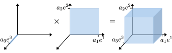
Figure 1: Multiplying the volume of a two-dimensional parallelotope and a one-dimensional parallelotope.

If $n$ is even, then taking $k=n/2$ in Thm. 7 yields the following result.

Corollary 10.

Let $A\in\mathbb{C}^{n\times n}$, with $n$ even. Let $r:=\binom{n}{n/2}$. Then

$$(UA^{(n/2)})^{T}A^{(n/2)}U=\det(A)I_{r}.$$ (24)

III-B Duality between additive compounds

The next result describes a duality relation between the additive compound matrices $A^{[k]}$ and $A^{[n-k]}$.

Theorem 11.

Let $A\in\mathbb{C}^{n\times n}$. Then

$$(A^{[k]})^{T}+U^{T}A^{[n-k]}U=\operatorname{tr}(A)I_{r}.$$ (25)

Proof:

Fix $\varepsilon>0$. Thm. 7 yields

$$\big{(}(I_{n}+\varepsilon A)^{(k)}\big{)}^{T}U^{T}(I_{n}+\varepsilon A)^{(n-k)}U =\det(I+\varepsilon A)I_{r}.$$ (26)

By (5), the term on the left-hand side of (26) is

$$(I_{r}+\varepsilon A^{[k]})^{T} U^{T}(I_{r}+\varepsilon A^{[n-k]})U+o(\varepsilon)$$

$$=I_{r}+\varepsilon(A^{[k]})^{T}+\varepsilon U^{T}A^{[n-k]}U+o(\varepsilon).$$

The term on the right-hand side of (26) is

$$\det(I+\varepsilon A)I_{r}=(1+\varepsilon\operatorname{tr}(A)+o(\varepsilon))I_{r}.$$

We conclude that

$$\varepsilon(A^{[k]})^{T}+\varepsilon U^{T}A^{[n-k]}U+o(\varepsilon)=(\varepsilon\operatorname{tr}(A)+o(\varepsilon))I_{r}.$$

Dividing both sides by $\varepsilon$, and taking $\varepsilon\to 0$ completes the proof. ∎

Example 7.

Consider the case $n=3$, $k=2$, and $A=\operatorname{diag}(a_{1},a_{2},a_{3})$. Then $A^{[2]}=\operatorname{diag}(a_{1}+a_{2},a_{1}+a_{3},a_{2}+a_{3})$, $U$ is as in (22), and $U^{T}AU=\operatorname{diag}(a_{3},a_{2},a_{1})$. Thus,

$$(A^{[2]})^{T}+U^{T}AU=(a_{1}+a_{2}+a_{3})I_{3}.$$

and this agrees with (25).

Remark 1.

Ref. [35] includes a result that is similar to Thm. 11. However, the result there uses a different matrix $U$, and is in fact wrong. A counterexample to the result as stated in Ref. [35] is, for example, the case $n=4$ and $k=2$.

Remark 2.

It follows from (25) that $A^{[n-1]}=\operatorname{tr}(A)I_{r}-U^{T}A^{T}U.$ This special case already appeared in [43], and has been used in the analysis of $(n-1)$-positive systems [50].

One implication of Thm. 11, that will be used below, is the following.

Corollary 12.

The matrices $(A^{[k]})^{T}$ and $U^{T}A^{[n-k]}U$ commute.

Proof:

It follows from Thm. 11 that $(A^{[k]})^{T}=\operatorname{tr}(A)I_{r}-U^{T}A^{[n-k]}U$, so

$$(A^{[k]})^{T}U^{T}A^{[n-k]}U =(\operatorname{tr}(A)I_{r}-U^{T}A^{[n-k]}U)U^{T}A^{[n-k]}U$$

$$=U^{T}A^{[n-k]}U(\operatorname{tr}(A)I_{r}-U^{T}A^{[n-k]}U)$$

$$=U^{T}A^{[n-k]}U(A^{[k]})^{T},$$

and this completes the proof. ∎

If $n$ is even then taking $k=n/2$ in Thm. 11 yields the following result.

Corollary 13.

Let $A\in\mathbb{C}^{n\times n}$, with $n$ even. Let $r:=\binom{n}{n/2}$. Then

$$(A^{[n/2]})^{T}+U^{T}A^{[n/2]}U=\operatorname{tr}(A)I_{r}.$$ (27)

III-C Duality between multiplicative compounds of the matrix exponential

The next result uses the duality relations above to derive a duality relation for the multiplicative compounds of the exponential of a matrix.

Theorem 14.

Let $A\in\mathbb{C}^{n\times n}$. Then

$$((\exp(A))^{(k)})^{T}=\exp(\operatorname{tr}(A))U^{T}\big{(}\exp(-A)\big{)}^{(n-k)}U.$$ (28)

Proof:

Let $D:=\big{(}(\exp(A))^{(k)}\big{)}^{T}U^{T}(\exp(A))^{(n-k)}U$. Using the identity $(\exp(A))^{(k)}=\exp(A^{[k]})$ (see, e.g., [34]) and the fact that $U^{T}=U^{-1}$ yields

$$U^{T}(\exp(A))^{(n-k)}U=U^{T}\exp(A^{[n-k]})U=\exp(U^{T}A^{[n-k]}U).$$

Thus, $D=(\exp(A^{[k]}))^{T}\exp(U^{T}A^{[n-k]}U)$, and applying Corollary 12 gives

$$D =\exp((A^{[k]})^{T}+U^{T}A^{[n-k]}U)$$

$$=\exp(\operatorname{tr}(A)I_{r})$$

$$=\exp(\operatorname{tr}(A))I_{r},$$

and this completes the proof. ∎

Example 8.

For $n=3$ and $k=2$, (28) becomes

$$((\exp(A))^{(2)})^{T}=\exp(\operatorname{tr}(A))U^{T}\exp(-A)U.$$

This provides an expression for all the $2$-minors of $\exp(A)$ that does not require to compute any minors.

III-D Duality between Log Norms of Additive Compounds

Proposition 15.

Let $A\in\mathbb{R}^{n\times n}$. Fix $k\in\{1,\ldots,n-1\}$, and let $r=\binom{n}{k}$. Let $U\in\{-1,0,1\}^{r\times r}$ be the matrix defined in (15). Then for any log norm $\mu:\mathbb{R}^{r\times r}\to\mathbb{R}$, we have:

$$\mu(A^{[k]})=\operatorname{tr}(A)+\mu_{U^{T}}(-(A^{[n-k]})^{T}).$$ (29)

Proof:

By (25),

$$A^{[k]}=\operatorname{tr}(A)I_{r}-U^{T}(A^{[n-k]})^{T}U.$$

Applying $\mu$ on both sides of this equation and using the fact that $\mu(cI+B)=c+\mu(B)$ for any scalar $c$ (see, e.g., [10]) yields:

$$\mu(A^{[k]}) =\operatorname{tr}(A)+\mu(-U^{T}(A^{[n-k]})^{T}U),$$

and this completes the proof. ∎

Corollary 16.

Let $A\in\mathbb{R}^{n\times n}$, with $n$ even. Let $r:=\binom{n}{n/2}$. Then for any log norm $\mu:\mathbb{R}^{r\times r}\to\mathbb{R}$, we have:

$$\mu(A^{[n/2]})=\operatorname{tr}(A)+\mu_{U^{T}}(-(A^{[n/2]})^{T}).$$ (30)

In particular, for any log norm $\mu_{p}$ induced by an $L_{p}$ norm, we have

$$\mu_{p}(A^{[n/2]})=\operatorname{tr}(A)+\mu_{q}(-(A^{[n/2]})),$$

and for the log norm induced by the $L_{2}$ norm:

$$\mu_{2}(A^{[n/2]})=\operatorname{tr}(A)+\mu_{2}(-A^{[n/2]}).$$ (31)

Example 9.

Consider $A\in\mathbb{R}^{(2\ell)\times(2\ell)}$, with $A=\operatorname{diag}(\lambda_{1},\dots,\lambda_{2\ell})$, and $\lambda_{1}\geq\dots\geq\lambda_{2\ell}$. Then $\operatorname{tr}(A)=\sum_{i=1}^{2\ell}\lambda_{i}$, $\mu_{2}(A^{[n/2]})=\sum_{i=1}^{\ell}\lambda_{i}$, and $\mu_{2}(-A^{[n/2]})=-\sum_{i=\ell+1}^{2\ell}\lambda_{i}$, so clearly (31) holds.

The formulas in Prop. 3 are not always easy to use. Indeed, the cardinality of the set $Q(k,n)$ is $\binom{n}{k}$ and this may be very large. In the next section, we use the duality relation (29) to derive a sufficient condition for $k$-contraction of non-linear dynamical systems which does not require calculating compounds of the Jacobian.

IV Compound-free sufficient condition for $k$-contraction

We begin by defining a new matrix operator.

Definition 4.

Given an integer $n\geq 1$, $k\in\{1,\dots,n\}$, $p\in\{1,2,\infty\}$, and an invertible matrix $T\in\mathbb{R}^{n\times n}$, the $k$-shifted log norm $\tau_{p,k}:\mathbb{R}^{n\times n}\to\mathbb{R}$ is defined by

$$\tau_{p,k}(A):=\operatorname{tr}(A)+(n-k)\mu_{q,T}(-A),$$ (32)

where $q$ is such that $q^{-1}+p^{-1}=1$.

Note that the name is justified by the equality $\tau_{p,k}(A)=\mu_{q,T}(\operatorname{tr}(A)I_{n}+(n-k)(-A))$. Note also that the matrix $U$ does not appear in the definition of $\tau_{p,k}$. As we will see below, this is due to Lemma 4,

We can now state the main result in this section.

Theorem 17.

For any $A\in\mathbb{R}^{n\times n}$, $k\in\{1,\dots,n\}$, $p\in\{1,2,\infty\}$, and an invertible matrix $T\in\mathbb{R}^{n\times n}$, we have

$$\mu_{p,T^{(k)}}(A^{[k]})\leq\tau_{p,k}(A).$$ (33)

In other words, $\tau_{p,k}(A)$ provides an upper bound on $\mu_{p,T^{(k)}}(A^{[k]})$ that does not require to compute any compounds. In particular, if $\tau_{p,k}(A)\leq-\eta<0$ then $\dot{x}=Ax$ is $k$-contracting with rate $\eta$ w.r.t. the scaled $L_{p}$ norm with weight matrix $T^{(k)}$. Similarly, if the Jacobian $J(t,x)$ of (10) satisfies

$$\tau_{p,k}(J(t,x))\leq-\eta<0,\text{ for all }t\geq 0,x\in\Omega$$

then (10) is $k$-contracting with rate $\eta$ w.r.t. the scaled $L_{p}$ norm with weight matrix $T^{(k)}$. Note that for $k=1$ this yields a non-standard sufficient condition for contraction w.r.t. $L_{p}$, namely,

$$\operatorname{tr}(J(t,x))+(n-1)\mu_{q,T}(-J(t,x))\leq-\eta<0$$

for all $t\geq 0$, $x\in\Omega$. More importantly, for $k>1$, this provides a sufficient condition for $k$-contraction that does not require computing any compounds.

The remainder of this section is devoted to the proof of Thm. 17. This requires the following auxiliary result that may be of independent interest.

Proposition 18.

Fix $A\in\mathbb{R}^{n\times n}$, $p\in\{1,2,\infty\}$, and $k,\ell\in\{1,\dots,n\}$ with $\ell\leq k$. Let $T\in\mathbb{R}^{n\times n}$ be invertible. Then

$$\frac{1}{k}\mu_{p,T^{(k)}}(A^{[k]}) \leq\frac{1}{\ell}\mu_{p,T^{(\ell)}}(A^{[\ell]}).$$ (34)

For example, for $\ell=1$ this gives $\mu_{p,T^{(k)}}(A^{[k]})\leq k\mu_{p,T}(A)$.

Proof:

We will use the following easy to verify fact. If $a_{1}\geq\dots\geq a_{n}$ and $k\in\{1,\dots,n-1\}$ then

$$\frac{1}{k}\sum_{i=1}^{k}a_{i}-\frac{1}{k+1}\sum_{i=1}^{k+1}a_{i}\geq\frac{a_{k}-a_{k+1}}{k+1}\geq 0.$$ (35)

We begin by proving (34) for $T=I_{n}$. We first consider the case $p=2$. Let $\lambda_{1}\geq\dots\geq\lambda_{n}$ denote the eigenvalues of $(A+A^{T})/2$. Then

$$\frac{\mu_{2}(A^{[k]})}{k}-\frac{\mu_{2}(A^{[k+1]})}{k+1} =\frac{1}{k}\sum_{i=1}^{k}\lambda_{i}-\frac{1}{k+1}\sum_{i=1}^{k+1}\lambda_{i}$$

$$\geq 0.$$

We now consider the case $p=1$. For any $\alpha\in Q(k,n)$, let $c_{\alpha,i}:=a_{ii}+\sum_{j\notin\alpha}|a_{ji}|$, with $i\in\{1,\dots,n\}$. Let $\beta:=\operatorname{argmax}_{\alpha\in Q(k,n)}\sum_{i\in\alpha}c_{\alpha,i}$. Let $i_{1},\dots,i_{k}\in\{1,\dots,n\}$ be such that $c_{\beta,i_{1}}\geq\dots\geq c_{\beta,i_{k}}$. Using Prop. 3 and (35) gives

$${k}^{-1}\mu_{1}\left(A^{[k]}\right) =\max_{\alpha\in Q(k,n)}{k}^{-1}\sum_{i\in\alpha}c_{\alpha,i}$$

$$={k}^{-1}(c_{\beta,i_{1}}+\dots+c_{\beta,i_{k}})$$

$$\leq{\ell}^{-1}(c_{\beta,i_{1}}+\dots+c_{\beta,i_{\ell}})$$

$$\leq\max_{\gamma\in Q(\ell,n)}{\ell}^{-1}\max_{i\in\gamma}(a_{ii}+\sum_{\begin{subarray}{c}j\notin\gamma\end{subarray}}|a_{ji}|)$$

$$={\ell}^{-1}\mu_{1}(A^{[\ell]}).$$

The proof for the case $p=\infty$ is similar and thus omitted. We conclude that

$$\frac{1}{k}\mu_{p}(A^{[k]}) \leq\frac{1}{\ell}\mu_{p}(A^{[\ell]}).$$

To complete the proof of (34), fix an invertible matrix $T$. Using (8) and the fact that $\mu_{T}(A)=\mu(TAT^{-1})$, we have that

$$k^{-1}\mu_{p,T^{(k)}}(A^{[k]}) =k^{-1}\mu_{p}((TAT^{-1})^{[k]})$$

$$\leq{\ell}^{-1}\mu_{p}((TAT^{-1})^{[\ell]})$$

$$={\ell}^{-1}\mu_{p,T^{(\ell)}}(A^{[\ell]}),$$

and this completes the proof. ∎

Example 10.

Let $A=I_{n}$ and fix $k\in\{1,\dots,n\}$. Then $A^{[k]}=kI_{r}$, so for any monotonic norm  and any invertible matrix $T$, we have $\mu_{p,T^{(k)}}(A^{[k]})=k$. Thus, inequality (34) holds with an equality, implying that the bound cannot be improved in general.

Remark 3.

Prop. 18 implies in particular that if the system (10) satisfies the infinitesimal condition for $\ell$-contraction with rate $\eta$ in (11) w.r.t. an $L_{p}$ norm scaled by $T^{(\ell)}$, with $p\in\{1,2,\infty\}$, then for any $k\in\{\ell,\ell+1,\dots,n\}$ it is $k$-contracting with rate $\frac{k}{\ell}\eta$ w.r.t. the same norm scaled by $T^{(k)}$ (see also [52, 3]). More generally, if a system is $\alpha$-contracting, with $\alpha>0$ real, then it is also $(\alpha+\varepsilon)$-contracting for any $\varepsilon\geq 0$ [54].

Remark 4.

Suppose that the system (10) satisfies the infinitesimal condition for $k$-contraction w.r.t. to $L_{p}$ for some $p\in\{1,2,\infty\}$. Then the system is also $n$-contractive, that is, $\operatorname{tr}(J(x))<0$ for all $x\in\Omega$. Suppose now that either $p=1$ or $p=\infty$. Since there exists at least one diagonal entry of $J(x)$ that is negative,

$$\mu_{p}(-J(x))>0,\text{ for all }x\in\Omega.$$ (36)

For $p=2$ we have $\mu_{2}(-J(x))=\lambda_{1}(-(J(x)+J^{T}(x))/2)$ and since

$$\operatorname{tr}(-(J(x)+J^{T}(x))/2)=\operatorname{tr}(-J(x))>0,$$

the formula for the $L_{2}$ log norm implies that Eq. (36) holds also when $p=2$. Thus, the sufficient condition for $k$-contraction in Thm. 17 is a trade-off between the negativity of $\operatorname{tr}(J(x))$ and the positivity of $(n-k)\mu_{p}(-J(x))$. In this case, if the sufficient condition for $k$-contraction holds, that is,

$$tr(J)+(n-k)\mu_{p}(-J)\leq-\eta<0,$$

then clearly

$$tr(J)+(n-(k+1))\mu_{p}(-J)\leq-\eta<0$$

so the sufficient condition for $(k+1)$-contraction also holds.

We can now prove Thm. 17.

Proof:

Using (9) and (8) yields

$$\mu_{p,T^{(k)}}(A^{[k]}) =\mu_{p}(T^{(k)}A^{[k]}(T^{(k)})^{-1})$$

$$=\mu_{p}((TAT^{-1})^{[k]})$$

$$=\mu_{q}(((TAT^{-1})^{[k]})^{T}),$$

where we used the duality relation for log norms in Lemma 5. Applying the duality for additive compounds in Thm. 11, and using the fact that $\mu(A+cI)=\mu(A)+c$ and $\mu(cI)=c$ for all log norms and any $c\in\mathbb{R}$, we get

$$\mu_{p,T^{(k)}}(A^{[k]}) =\operatorname{tr}(TAT^{-1})+\mu_{q}(-U^{T}(TAT^{-1})^{[n-k]}U)$$

$$=\operatorname{tr}(A)+\mu_{q}(-(TAT^{-1})^{[n-k]})$$

$$=\operatorname{tr}(A)+\mu_{q,T^{(n-k)}}(-A^{[n-k]}),$$ (37)

where we used Lemma 4. Applying Prop. 18 yields

$$\mu_{p,T^{(k)}}(A^{[k]})\leq\operatorname{tr}(A)+(n-k)\mu_{q,T}(-A),$$ (38)

and this completes the proof. ∎

The next result summarizes some properties of the $k$-shifted log norm $\tau_{p,k}$. The proof follows from Definition 4, linearity of the trace operator, and known properties of log norms (see, e.g., [10]).

Proposition 19.

Fix $A,B\in\mathbb{R}^{n\times n}$, $k\in\{1,\dots,n\}$, and $p\in\{1,2,\infty\}$. Then

1. $\tau_{p,k}(0)=0$.

2. $|\tau_{p,k}(A)-\tau_{p,k}(B)|\leq|\operatorname{tr}(A-B)|+(n-k)\|A-B\|_{q,T}$.

3. $\tau_{p,k}(A+B)\leq\tau_{p,k}(A)+\tau_{p,k}(B)$.

4. $\tau_{p,k}(cA)=c\tau_{p,k}(A)$, for any $c\in\mathbb{R}_{+}$.

5. $\tau_{p,k}(A+cI_{n})=\tau_{p,k}(A)+kc$, for any $c\in\mathbb{R}$. In particular,

   $$\tau_{p,k}(I_{n})=k,\quad\tau_{p,k}(-I_{n})=-k.$$

6. $$\operatorname{tr}(A)-(n-k)\|A\|_{q,T} \leq\operatorname{tr}(A)-(n-k)\mu_{q,T}(A)$$

   $$\leq\tau_{p,k}(A)$$

   $$\leq\operatorname{tr}(A)+(n-k)\|A\|_{q,T}.$$

7. $\tau_{p,k}(rA+(1-r)B)\leq r\tau_{p,k}(A)+(1-r)\tau_{p,k}(B)$, for any $r\in[0,1]$.

In particular, $\tau_{p,k}$ is continuous, sub-additive, positively homogeneous of degree one, and convex. The latter property implies that it is possible to verify the sufficient condition for $k$-contraction in Thm. 17 for a polytope of dynamical systems by checking only the vertices of this polytope.

V Applications

We now describe several applications of Thm. 17. In particular, we show how it can be used to prove $k$-contraction in $n$-dimensional nonlinear systems without computing any $k$-compounds. However, it is instructive to begin with LTI systems.

V-A $k$-contraction in LTI systems

Consider the LTI system

$$\dot{x}(t)=Ax(t),$$ (39)

with $A\in\mathbb{R}^{n\times n}$.

Suppose first that $A=\operatorname{diag}(\lambda_{1},\dots,\lambda_{n})$, with

$$\lambda_{1}\geq\dots\geq\lambda_{n}.$$ (40)

Fix $p\in\{1,2,\infty\}$. Then

$$\tau_{p,k}(A) =\operatorname{tr}(A)+(n-k)\mu_{q}(-A)$$

$$=\lambda_{1}+\dots+\lambda_{n}-(n-k)\lambda_{n}$$

$$=-(n-k-1)\lambda_{n}+\lambda_{1}+\dots+\lambda_{n-1}.$$

Combining this with (40) implies that $\tau_{p,k}(A)<0$ iff

$$\lambda_{1}+\dots+\lambda_{n-1}<(n-k-1)\lambda_{n}<0.$$ (41)

If $k=n-1$ then this is equivalent to $\lambda_{1}+\dots+\lambda_{n-1}<0$ which is indeed a necessary and sufficient condition for $(n-1)$-contraction of (39). For $k<n-1$ condition (41) requires that the sum of the first $n-1$ eigenvalues is “negative enough” to guarantee $k$-contraction.

Now assume that $A$ is not necessarily diagonal. Let $\lambda_{1},\dots,\lambda_{n}$ denote the eigenvalues of $A$, ordered such that $(\lambda_{1})\geq\dots\geq(\lambda_{n})$. Then (32) with $T=I_{n}$ yields

$$\tau_{p,k}(A)=\operatorname{tr}(A)+(n-k)\mu_{q}(-A).$$

Using the bound $\mu(-A)\geq(-\lambda_{n})$ gives

$$\tau_{p,k}(A) \geq\sum_{i=1}^{n}(\lambda_{i})+(n-k)(-\lambda_{n})$$

$$\geq n(\lambda_{n})-(n-k)(\lambda_{n})$$

$$=k(\lambda_{n}),$$

so in particular if $\tau_{p,k}(A)<0$ then we must have that $(\lambda_{n})<0$. In other words, if the sufficient $k$-contractivity condition holds then $A$ is not “too unstable” in the sense that it has at least one eigenvalue with a negative real part.

Recall that for the LTI system (39) $k$-contraction implies that every sum of $k$ eigenvalues of $A$ has a negative real part [52]. Combining this with Thm. 17 yields the following result.

Corollary 20.

Let $A\in\mathbb{R}^{n\times n}$. Suppose that there exist an invertible matrix $T\in\mathbb{R}^{n\times n}$, $k\in\{1,\dots,n\}$, and $q\in\{1,2,\infty\}$ such that

$$\operatorname{tr}(A)+(n-k)\mu_{q,T}(-A)<0.$$

Then every sum of $k$ eigenvalues of $A$ has a negative real part.

The next result shows how Thm. 17 can be used to derive a “$k$-trace dominance condition” guaranteeing $k$-contraction.

Corollary 21.

Fix $k\in\{1,\dots,n\}$. If there exist $d_{1},\dots,d_{n}>0$ such that

$$-(n-k-1)a_{ii}+\sum_{j\not=i}\Big{(}a_{jj}+(n-k)\frac{d_{j}}{d_{i}}|a_{ji}|\Big{)}\leq-\eta<0,$$ (42)

for all $i\in\{1,\dots,n\}$, then the LTI (39) is $k$-contractive with rate $\eta$ w.r.t. the scaled norm $|\cdot|_{\infty,D}$, where $D:=\operatorname{diag}(d_{1},\dots,d_{n})$.

Note that for $k=n$ condition (42) becomes

$$\operatorname{tr}(A)\leq-\eta<0,$$

whereas for $k=n-1$ and $D=I_{n}$ it becomes

$$\operatorname{tr}(A)-a_{pp}+\sum_{j\not=p}|a_{jp}|\leq-\eta<0,\text{ for all }p\in\{1,\dots,n\}.$$

Proof:

We prove Corollary 21 for the case $D=I_{n}$. The general case follows by replacing $A$ with $DAD^{-1}$. Consider

$$\tau_{\infty,k}(A) =\operatorname{tr}(A)+(n-k)\mu_{1}(-A)$$

$$=\sum_{i=1}^{n}a_{ii}+(n-k)\max(c_{1},\dots,c_{n}),$$

where $c_{i}:=-a_{ii}+\sum_{j\not=i}|a_{ji}|$, that is, the sum of the entries in column $i$ of $(-A)$, with off-diagonal entries taken with absolute value. For concreteness, assume that $\max(c_{1},\dots,c_{n})=c_{1}$, that is,

$$-a_{11}+\sum_{j\not=1}|a_{j1}|\geq-a_{\ell\ell}+\sum_{j\not=\ell}|a_{j\ell}|,\text{ for all }\ell\geq 1.$$

Then

$$\tau_{\infty,k}(A) =\sum_{i=1}^{n}a_{ii}+(n-k)(-a_{11}+\sum_{j\not=1}|a_{j1}|)$$

$$=-(n-k-1)a_{11}+\sum_{j\not=1}(a_{jj}+(n-k)|a_{j1}|).$$

Comparing this with (42) completes the proof. ∎

V-B $k$-contraction in LTV systems

Applying Thm. 17 to prove $k$-contraction requires bounding $\mu_{q,T}(-J(t,x))$ from above. For the case of an LTV system and the $L_{2}$ norm (i.e., $q=2$), a useful bound was derived in [44].

Lemma 22.

[44] Consider the matrix LTV system

$$\dot{X}(t)=A(t)X(t),\quad X(0)=I,$$ (43)

with $A:\mathbb{R}_{+}\to\mathbb{R}^{n\times n}$ continuous. Suppose that there exist $Q\succ 0$ and a continuous function $\theta:\mathbb{R}_{+}\to\mathbb{R}$ such that

$$A^{T}(t)Q+QA(t)+2\theta(t)Q\succeq 0,\text{ for all }t\geq 0.$$ (44)

Let $P\succ 0$ be such that $P^{2}=Q$. Then

$$\mu_{2,P}(-A(t))\leq\theta(t),\text{ for all }t\geq 0.$$ (45)

The proof follows from multiplying (44) by $P^{-1}$ on the left- and right-hand sides.

Combining this bound with Thm. 17 yields the following result.

Proposition 23.

Consider the matrix LTV system (43) and suppose that the conditions in Lemma 22 hold. Fix $k\in\{1,\dots,n\}$. If

$$\operatorname{tr}(A(t))+(n-k)\theta(t)\leq-\eta<0,\text{ for all }t\geq 0$$

then the LTV system is $k$-contracting with rate $\eta$ w.r.t. the scaled $L_{2}$ norm $|\cdot|_{2,P}$.

Proof:

Consider

$$\tau_{2,k}(A(t))=\operatorname{tr}(A(t))+(n-k)\mu_{2,P}(-A(t)).$$

Combining this with (45) gives

$$\tau_{2,k}(A(t))\leq\operatorname{tr}(A(t))+(n-k)\theta(t),$$

and applying Thm. 17 completes the proof. ∎

Example 11.

Consider the LTI (39), but with an uncertainty in the matrix $A$. A standard approach for modeling this is to assume that $A$ is constant, unknown, and belongs to the convex hull of a set of $s$ known matrices $A_{1},\dots,A_{s}$. We assume that all the matrices have the same trace

$$r:=\operatorname{tr}(A_{i}),\quad i=1,\dots,s.$$

This is a typical case, for example, in modeling biological interaction networks (also known as chemical reaction networks), see, e.g., [3]. Prop. 23 implies that if we can find $Q\succ 0$ and $\theta\in\mathbb{R}$ such that

$$A_{i}^{T}Q+QA_{i}+2\theta Q\succeq 0,\text{ for all }i\in\{1,\dots,s\},$$

and

$$r+(n-k)\theta\leq-\eta<0,$$

then the uncertain LTI is $k$-contractive. We emphasize again that this does not require computing any compounds.

V-C $k$-contraction in $n$-dimensional Hopfield Neural Networks

Consider the Hopfield neural network [16]

$$\dot{x}_{i}(t)=-\frac{x_{i}(t)}{r_{i}}+\sum_{j=1}^{n}w_{ij}\phi_{j}(x_{j}(t))+u_{i},\quad i=1,\dots,n,$$ (46)

where $r_{i}>0$, $u_{i}$ is a constant input to neuron $i$, $\phi_{j}:\mathbb{R}\to\mathbb{R}$ is the activation function of neuron $j$, and $W=\{w_{ij}\}_{i,j=1}^{n}$ is the network connection matrix. We assume that every $\phi_{i}$ is $C^{1}$.

The stability of (46) has been studied extensively, e.g., via Lyapunov analysis in [32, 20, 13]. Ref. [11] seems to be the first application of log norms to analyze Hopfield neural networks; later works include [40, 8] on contractivity w.r.t. non-Euclidean norms, and [41, 22] on contractivity w.r.t. Euclidean norms. However, in many applications the network admits more than a single equilibrium. For example, in using a Hopfield network as an associative memory [16, 23], every stored pattern corresponds to an equilibrium. Thus, if the network stores more than a single memory than it cannot be contractive w.r.t. any norm.

The Jacobian of (46) is

$$J(x)=-\operatorname{diag}\big{(}r_{1}^{-1},\dots,r_{n}^{-1})+W\operatorname{diag}(\phi_{1}^{\prime}(x_{1}),\dots,\phi_{n}^{\prime}(x_{n})\big{)},$$ (47)

where $\phi_{i}^{\prime}(x_{i}):=\frac{d}{dx}\phi_{i}(x)|_{x=x_{i}}$. Thm. 17 allows to derive a sufficient condition for $k$-contraction of the Hopfield network without computing compounds. One possibility is to assume that the $\phi_{i}^{\prime}$s are bounded, and then apply the same approach as in Corollary 21.

Proposition 24.

Consider the Hopfield network (46). Assume that the neuron activation functions satisfy

$$0\leq m_{i}\leq|\phi_{i}^{\prime}(z)|\leq M_{i},\text{ for all }z\in\mathbb{R}\text{ and }i\in\{1,\dots,n\}.$$ (48)

If there exist $d_{1},\dots,d_{n}>0$ such that

$$-(n-k-1)(-r_{i}^{-1}-m_{i}|w_{ii}|)$$

$$+\sum_{j\not=i}\Big{(}-r_{j}^{-1}+M_{j}|w_{jj}|+(n-k)\frac{d_{j}}{d_{i}}M_{i}|w_{ji}|\Big{)}\leq-\eta<0,$$ (49)

for all $i\in\{1,\dots,n\}$, then (46) is $k$-contractive with rate $\eta$ w.r.t. the scaled norm $|\cdot|_{\infty,D}$, with $D:=\operatorname{diag}(d_{1},\dots,d_{n})$.

A common choice for the activation functions in neural network models is $\phi_{i}(z)=a_{i}\tanh(b_{i}z)$ and then clearly condition (48) indeed holds. Note also that if we set $r_{1}=\dots=r_{n}=r$ then (24) will hold for any $r>0$ sufficiently small. This makes sense, as a smaller $r$ makes (46) “more stable”. We emphasize again that condition (24) does not require to compute any compounds of the Jacobian $J(x)$ in (47).

Proof:

Consider

$$\tau_{\infty,k}(J(x))(J(x)) =\operatorname{tr}(J(x))+(n-k)\mu_{1}(-J(x))$$

$$=\sum_{i=1}^{n}(w_{ii}\phi_{i}^{\prime}(x_{i})-r_{i}^{-1})$$

$$+(n-k)\max(c_{1}(x),\dots,c_{n}(x)),$$

where

$$c_{i}(x):=r_{i}^{-1}-w_{ii}\phi^{\prime}_{i}+\sum_{j\not=i}|w_{ji}\phi^{\prime}_{i}|.$$

For concreteness, assume that $\max(c_{1}(x),\dots,c_{n}(x))=c_{1}(x)$. Then

$$\tau_{\infty,k}(J(x)) =-(n-k-1)(w_{11}\phi_{1}^{\prime}(x_{1})-r_{1}^{-1})$$

$$+\sum_{i\not=1}(w_{ii}\phi_{i}^{\prime}(x_{i})-r_{i}^{-1})+(n-k)\sum_{j\not=1}|w_{ji}\phi^{\prime}_{i}|.$$

Applying (48) gives

$$\tau_{\infty,k}(J(x)) \leq-(n-k-1)(-|w_{11}|m_{1}-r_{1}^{-1})$$

$$+\sum_{i\not=1}(|w_{ii}|M_{i}-r_{i}^{-1})+(n-k)\sum_{j\not=1}|w_{ji}|M_{i}$$

for all $x$, and this completes the proof. ∎

Example 12.

Consider (46) with $|w_{ij}|=1$ for all $i,j$ (i.e., a binary weight matrix), $r_{i}=r$ and $\phi_{i}(z)=\tanh(z)$ for all $i$, that is,

$$\dot{x}_{i}=-\frac{x_{i}}{r}+\sum_{j=1}^{n}(\pm 1)\tanh(x_{j})+u_{i},\quad i=1,\dots,n,$$ (50)

where $\pm 1$ indicates a value that can be either $-1$ or $+1$. For large $r$, this system may have more than a single equilibrium and may not be contractive w.r.t. any norm. We apply Prop. 24 with $D=I_{n}$ to find a sufficient condition for $k$-contraction. In this case, $m_{i}=0$ and $M_{i}=1$ for all $i$, and (24) becomes

$$-kr^{-1}+(n-1)(n-k+1)\leq-\eta<0.$$

Thus, a sufficient condition for $k$-contraction is

$$r<\frac{k}{(n-1)(n-k+1)}.$$ (51)

Note also that this did not require to compute and analyze $J^{[k]}(x)$ which in this case is an $\binom{n}{k}\times\binom{n}{k}$ state-dependent matrix.

For example, if we require $(n-1)$-contraction then (51) becomes the condition $r<1/2$. As a specific example, take $n=3$, $w_{ij}=1$ for all $i,j$, $r_{i}=0.49$ and $f_{i}(z)=\tanh(z)$ for all $i$, that is,

$$\dot{x}_{i}=-\frac{x_{1}}{0.49}+\sum_{i=1}^{3}\tanh(x_{i}),\quad i=1,2,3.$$ (52)

This system admits at least three equilibrium points:

$$e^{1}=0,\;e^{2}\approx 1.2447\begin{bmatrix}1&1&1\end{bmatrix}^{T},\;e^{3}=-e^{2},$$ (53)

so it is not contractive w.r.t any norm. It satisfies the sufficient condition for $2$-contraction (namely, $r<1/2$), so the results of Muldowney and Li [34, 26] imply that every bounded solution converges to an equilibrium point. It is clear from (52) that all trajectories of the system are bounded. Fig. 2 depicts several trajectories of this system from random initial conditions. It may be seen that all the trajectories indeed converge to either $e^{2}$ or $e^{3}$. Note that in this example, $n=3$ and $k=2$, so we can easily compute and analyze $J^{[2]}(x)$ directly, but our goal is merely to demonstrate the bound derived in Thm. 17.

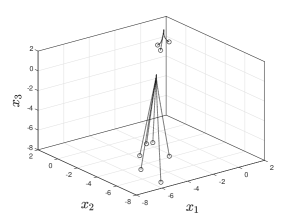
Figure 2: Trajectories of the Hopfield network in (52). Initial conditions are marked by o.

V-D Local stability of an equilibrium of a non-linear dynamical system

Li and Wang [27] proved that a matrix $A\in\mathbb{R}^{n\times n}$ is Hurwitz iff the following two conditions hold:

$$A^{[2]}\text{ is Hurwitz and }(-1)^{n}\det(A)>0.$$ (54)

The proof is based on the fact that every eigenvalue of $A^{[2]}$ is the sum of two eigenvalues of $A$. This result was applied to prove the local stability of the endemic equilibrium $e$ in an SEIR model with a varying total population size [27] by verifying that $J(e)$, the Jacobian of the vector field evaluated at the equilibrium, is Hurwitz. In this case, $J(e)\in\mathbb{R}^{3\times 3}$ depends on various parameters of the model and verifying that $J(e)$ is Hurwitz using the Routh–Hurwitz stability criterion is non-trivial. However, in general verifying that (54) holds requires computing $A^{[2]}$ which is a matrix of dimensions $\binom{n}{2}\times\binom{n}{2}$. The next result uses the operator $\tau_{p,k}$ and does not require to compute $2$-compounds.

Corollary 25.

Let $e\in\mathbb{R}^{n}$ be an equilibrium of the system $\dot{x}=f(x)$, with $f\in C^{1}$. Let $J(x):=\frac{\partial}{\partial x}f(x)$. If there exist $p\in\{1,2,\infty\}$ and an invertible matrix $T\in\mathbb{R}^{n\times n}$ such that

$$\tau_{p,2}(J(e))=\operatorname{tr}(J(e))+(n-2)\mu_{q,T}(-J(e))<0,$$ (55)

where $p^{-1}+q^{-1}=1$, and

$$(-1)^{n}\det(J(e))>0$$ (56)

then $e$ is locally asymptotically stable.

Proof:

By Thm. 17, Eq. (55) implies that $\mu((J(e))^{[2]})<0$, and combining this with (56) implies that $J(e)$ is Hurwitz. ∎

Note that conditions (55) and (56) do not require to compute $(J(e))^{[2]}$.

As a simple example consider again the Hopfield network in (52) and the equilibrium points in (53). We already know that condition (55) holds at any point in the state-space, so we only need to check condition (56), that is,

$$\det(J(e))<0.$$ (57)

Using (47) gives

$$J(x) =-\operatorname{diag}(1/0.49,1/0.49,1/0.49)$$

$$+\begin{bmatrix}1-\tanh^{2}(x_{1})&1-\tanh^{2}(x_{2})&1-\tanh^{2}(x_{3})\\ 1-\tanh^{2}(x_{1})&1-\tanh^{2}(x_{2})&1-\tanh^{2}(x_{3})\\ 1-\tanh^{2}(x_{1})&1-\tanh^{2}(x_{2})&1-\tanh^{2}(x_{3})\end{bmatrix}.$$

It follows that $\det(J(x))=(-1/0.49)^{2}((-1/0.49)+3-\sum_{i=1}^{3}\tanh^{2}(x_{i}))$. In particular, $\operatorname{sgn}(\det(J(e^{1})))>0$ and $\operatorname{sgn}(\det(J(e^{2})))<0$. Thus, $e^{2}$ is locally asymptotically stable, and $e^{1}$ is not locally asymptotically stable.

VI Conclusion

Contraction theory plays an important role in systems and control theory. However, many systems cannot be analyzed using contraction theory. For example, systems with more than a single equilibrium are not contractive w.r.t. any norm.

The notion of $k$-contraction provides a useful geometric generalization of contraction theory, but the standard sufficient condition for $k$-contraction of $n$-dimensional systems may be difficult to verify, as it is based on a compound matrix with dimensions $\binom{n}{k}\times\binom{n}{k}$. We derived duality relations between compound matrices, and used these to develop a sufficient condition for $k$-contraction that does not require to compute any compounds. We demonstrated our approach by deriving a sufficient condition for $k$-contraction of a Hopfield neural network. In the particular case where $k=2$ this implies that every bounded solution of the network converges to an equilibrium, which is of course a useful property when using the network as an associative memory [23]. We believe that the sufficient conditions for $k$-contraction derived here will prove useful in more applications.

Several results in this paper are proved for $L_{p}$ norms, with $p\in\{1,2,\infty\}$. It may be of interest to try and generalize the proofs to any $L_{p}$ norm. Another interesting direction for future research is to extend the tools described here to control synthesis. In other words, to systematically design a controller such that the closed-loop system satisfies the sufficient condition for $k$-contraction.

Omri Dalin received the BSc degree in Mech. Eng. from Tel Aviv University, in 2020. He is currently an MSc student at the Dept. of Mech. Eng. at Tel Aviv University.

Ron Ofir (Student Member, IEEE) received his BSc degree (cum laude) in Elec. Eng. from the Technion-Israel Institute of Technology in 2019. He is currently pursuing his Ph.D. degree in the Vitebri Faculty of Electrical Engineering, Technion- Israel Institute of Technology. His current research interests include contraction theory and its applications in dynamics and control of power systems.

Eyal Bar-Shalom received the BSc degree (cum laude) and MSc degree (cum laude) in Elec. Eng. from Tel Aviv University, in 2012 and 2019, respectively. He is currently a PhD student at the Dept. of Elec. Eng. at Tel Aviv University.

Alexander Ovseevich received his MSc in Mathematics from the Moscow State University in 1973, and PhD in Mathematics from the Leningrad division of the Steklov mathematical institute, RAS in 1976. He got a degree of the doctor of Phys.-Math. Sciences from the Institute for Problems in Mechanics, Moscow, Russia in 1997. He worked in the Institute for Problems in Mechanics from 1978 to 2022 as a senior research fellow and a leading research fellow. In 2022 he joined the Dept. of Elec. Eng.-Systems, Tel Aviv University, where he is currently a research assistant. His research interests include many topics from Number Theory to Mathematical Physics and Control Theory.

Francesco Bullo (Fellow, IEEE) is a Distinguished Professor of Mechanical Engineering at the University of California, Santa Barbara. He was previously associated with the University of Padova, the California Institute of Technology, and the University of Illinois. He served as IEEE CSS President and as SIAG CST Chair. His research focuses on contraction theory, network systems and distributed control with application to machine learning, power grids, social networks, and robotics. He is the coauthor of “Geometric Control of Mechanical Systems” (Springer, 2004), “Distributed Control of Robotic Networks” (Princeton, 2009), “Lectures on Network Systems” (KDP, 2022, v1.6), and ”Contraction Theory for Dynamical Systems” (KDP, 2022, v1.0). He is a Fellow of ASME, IFAC, and SIAM.

Michael Margaliot received the BSc (cum laude) and MSc degrees in Elec. Eng. from the Technion-Israel Institute of Technology-in 1992 and 1995, respectively, and the PhD degree (summa cum laude) from Tel Aviv University in 1999. He was a post-doctoral fellow in the Dept. of Theoretical Math. at the Weizmann Institute of Science. In 2000, he joined the Dept. of Elec. Eng.-Systems, Tel Aviv University, where he is currently a Professor. His research interests include the stability analysis of differential inclusions and switched systems, optimal control theory, computation with words, Boolean control networks, contraction theory, $k$-positive systems, and systems biology. He is co-author of New Approaches to Fuzzy Modeling and Control: Design and Analysis, World Scientific, 2000 and of Knowledge-Based Neurocomputing, Springer, 2009. He served as an Associate Editor of IEEE Transactions on Automatic Control during 2015-2017.

References

• [1] Z. Aminzare and E. D. Sontag, “Contraction methods for nonlinear systems: A brief introduction and some open problems,” in Proc. 53rd IEEE Conf. on Decision and Control, Los Angeles, CA, 2014, pp. 3835–3847.
• [2] V. Andrieu, B. Jayawardhana, and L. Praly, “Transverse exponential stability and applications,” IEEE Trans. Automat. Control, vol. 61, no. 11, pp. 3396–3411, 2016.
• [3] D. Angeli, M. Ali Al-Radhawi, and E. Sontag, “A robust Lyapunov criterion for non-oscillatory behaviors in biological interaction networks,” IEEE Trans. Automat. Control, vol. 67, no. 7, pp. 3305–3320, 2022.
• [4] D. Angeli, J. E. Ferrell, and E. D. Sontag, “Detection of multistability, bifurcations, and hysteresis in a large class of biological positive-feedback systems,” Proceedings of the National Academy of Sciences, vol. 101, no. 7, pp. 1822–1827, 2004.
• [5] E. Bar-Shalom, O. Dalin, and M. Margaliot, “Compound matrices in systems and control theory: a tutorial,” 2022. [Online]. Available: https://arxiv.org/abs/2204.00676
• [6] F. L. Bauer, J. Stoer, and C. Witzgall, “Absolute and monotonic norms,” Numer. Math., vol. 3, pp. 257–264, 1961.
• [7] F. Bullo, Contraction Theory for Dynamical Systems.   Kindle Direct Publishing, 2022. [Online]. Available: http://motion.me.ucsb.edu/book-ctds
• [8] A. Davydov, A. V. Proskurnikov, and F. Bullo, “Non-Euclidean contractivity of recurrent neural networks,” in American Control Conference, May 2022.
• [9] C. Desoer and H. Haneda, “The measure of a matrix as a tool to analyze computer algorithms for circuit analysis,” IEEE Trans. Circuit Theory, vol. 19, no. 5, pp. 480–486, 1972.
• [10] C. A. Desoer and M. Vidyasagar, Feedback Synthesis: Input-Output Properties.   Philadelphia: SIAM, 2009.
• [11] Y. Fang and T. G. Kincaid, “Stability analysis of dynamical neural networks,” IEEE Transactions on Neural Networks, vol. 7, no. 4, pp. 996–1006, 1996.
• [12] H. Flanders, “A note on the Sylvester-Franke theorem,” The American Mathematical Monthly, vol. 60, no. 8, pp. 543–545, 1953.
• [13] M. Forti and A. Tesi, “New conditions for global stability of neural networks with application to linear and quadratic programming problems,” IEEE Transactions on Circuits and Systems I: Fundamental Theory and Applications, vol. 42, no. 7, pp. 354–366, 1995.
• [14] M. Giaccagli, V. Andrieu, S. Tarbouriech, and D. Astolfi, “Infinite gain margin, contraction and optimality: an LMI-based design,” Euro. J. Control, 2022, to appear.
• [15] C. Grussler and R. Sepulchre, “Variation diminishing linear time-invariant systems,” Automatica, vol. 136, p. 109985, 2022.
• [16] J. J. Hopfield, “Neural networks and physical systems with emergent collective computational abilities,” Proceedings of the National Academy of Sciences, vol. 79, no. 8, p. 2554–2558, 1982.
• [17] R. A. Horn and C. R. Johnson, Matrix Analysis, 2nd ed.   Cambridge University Press, 2013.
• [18] S. Jafarpour, P. Cisneros-Velarde, and F. Bullo, “Weak and semi-contraction for network systems and diffusively coupled oscillators,” IEEE Trans. Automat. Control, vol. 67, no. 3, pp. 1285–1300, 2022.
• [19] J. Jiang and J. Shi, “Bistability dynamics in structured ecological models,” in Spatial Ecology, S. Cantrell, C. Cosner, and S. Ruan, Eds.   Chapman and Hall, 2009.
• [20] E. Kaszkurewicz and A. Bhaya, “On a class of globally stable neural circuits,” IEEE Transactions on Circuits and Systems I: Fundamental Theory and Applications, vol. 41, no. 2, pp. 171–174, 1994.
• [21] I. Z. Kiss, J. C. Miller, and P. L. Simon, Mathematics of Epidemics on Networks: From Exact to Approximate Models.   Springer, 2017.
• [22] L. Kozachkov, M. Ennis, and J.-J. E. Slotine, “Recursive construction of stable assemblies of recurrent neural networks,” 2021. [Online]. Available: https://arxiv.org/abs/2106.08928
• [23] D. Krotov and J. J. Hopfield, “Dense associative memory for pattern recognition,” in Advances in Neural Information Processing Systems, D. Lee, M. Sugiyama, U. Luxburg, I. Guyon, and R. Garnett, Eds., vol. 29.   Curran Associates, Inc., 2016.
• [24] M. Laurent and N. Kellershohn, “Multistability: a major means of differentiation and evolution in biological systems,” Trends Biochem Sci., vol. 24, no. 11, pp. 418–22, 1999.
• [25] M. Y. Li, J. R. Graef, L. Wang, and J. Karsai, “Global dynamics of a SEIR model with varying total population size,” Mathematical Biosciences, vol. 160, no. 2, pp. 191–213, 1999.
• [26] M. Y. Li and J. S. Muldowney, “On R. A. Smith’s autonomous convergence theorem,” Rocky Mountain J. Math., vol. 25, no. 1, pp. 365–378, 1995.
• [27] M. Y. Li and L. Wang, “A criterion for stability of matrices,” J. Mathematical Analysis and Applications, vol. 225, no. 1, pp. 249–264, 1998.
• [28] W. Lohmiller and J.-J. E. Slotine, “On contraction analysis for non-linear systems,” Automatica, vol. 34, pp. 683–696, 1998.
• [29] M. Margaliot, E. D. Sontag, and T. Tuller, “Entrainment to periodic initiation and transition rates in a computational model for gene translation,” PLoS ONE, vol. 9, no. 5, p. e96039, 2014.
• [30] M. Margaliot and E. D. Sontag, “Revisiting totally positive differential systems: A tutorial and new results,” Automatica, vol. 101, pp. 1–14, 2019.
• [31] M. Margaliot, E. D. Sontag, and T. Tuller, “Contraction after small transients,” Automatica, vol. 67, pp. 178–184, 2016.
• [32] A. N. Michel, J. A. Farrell, and W. Porod, “Qualitative analysis of neural networks,” IEEE Transactions on Circuits and Systems, vol. 36, no. 2, pp. 229–243, 1989.
• [33] T. Muir, A Treatise on the Theory of Determinants.   London: Longmans, 1933, revised edition.
• [34] J. S. Muldowney, “Compound matrices and ordinary differential equations,” The Rocky Mountain Journal of Mathematics, pp. 857–872, 1990.
• [35] ——, “Compound matrices and applications,” 1998. [Online]. Available: https://sites.ualberta.ca/~mathirl/IUSEP/IUSEP_2019/lecture_notes/compound_ula.pdf
• [36] R. Ofir and M. Margaliot, “The multiplicative compound of a matrix pencil with applications to difference-algebraic equations,” 2021. [Online]. Available: arXivpreprintarXiv:2111.01419
• [37] R. Ofir, M. Margaliot, Y. Levron, and J.-J. Slotine, “A sufficient condition for $k$-contraction of the series connection of two systems,” IEEE Trans. Automat. Control, vol. 67, no. 9, pp. 4994–5001, 2022.
• [38] A. Pavlov, N. van de Wouw, and H. Nijmeijer, “Frequency response functions and Bode plots for nonlinear convergent systems,” in Proc. 45th IEEE Conf. on Decision and Control, 2006, pp. 3765–3770.
• [39] A. V. Pavlov, N. van de Wouw, and H. Nijmeijer, Uniform Output Regulation of Nonlinear Systems: A Convergent Dynamics Approach.   Boston, MA: Birkhauser, 2006.
• [40] H. Qiao, J. Peng, and Z.-B. Xu, “Nonlinear measures: a new approach to exponential stability analysis for Hopfield-type neural networks,” IEEE Trans. Neural Networks, vol. 12, no. 2, pp. 360–370, 2001.
• [41] M. Revay, R. Wang, and I. R. Manchester, “Lipschitz bounded equilibrium networks,” 2020. [Online]. Available: https://arxiv.org/abs/2010.01732
• [42] G. Russo, M. di Bernardo, and E. D. Sontag, “Global entrainment of transcriptional systems to periodic inputs,” PLOS Computational Biology, vol. 6, p. e1000739, 2010.
• [43] B. Schwarz, “Totally positive differential systems,” Pacific J. Math., vol. 32, no. 1, pp. 203–229, 1970.
• [44] R. A. Smith, “Some applications of Hausdorff dimension inequalities for ordinary differential equations,” Proc. Royal Society of Edinburgh: Section A Mathematics, vol. 104, no. 3-4, pp. 235–259, 1986.
• [45] E. D. Sontag, “Contractive systems with inputs,” in Perspectives in Mathematical System Theory, Control, and Signal Processing: A Festschrift in Honor of Yutaka Yamamoto on the Occasion of his 60th Birthday, J. C. Willems, S. Hara, Y. Ohta, and H. Fujioka, Eds.   Berlin, Heidelberg: Springer, 2010, pp. 217–228.
• [46] T. StrĂśm, “On logarithmic norms,” SIAM J. Numerical Analysis, vol. 12, no. 5, pp. 741–753, 1975.
• [47] H. Tsukamoto and S. J. Chung, “Learning-based robust motion planning with guaranteed stability: A contraction theory approach,” IEEE Robotics and Automation Letters, vol. 6, no. 4, pp. 6164–6171, 2021.
• [48] M. Vidyasagar, Nonlinear Systems Analysis.   SIAM, 2002.
• [49] W. Wang and J. J. E. Slotine, “On partial contraction analysis for coupled nonlinear oscillators,” Biological Cybernetics, vol. 92, no. 1, 2005.
• [50] E. Weiss and M. Margaliot, “A generalization of linear positive systems with applications to nonlinear systems: Invariant sets and the PoincarĂŠ-Bendixson property,” Automatica, vol. 123, p. 109358, 2021.
• [51] P. M. Wensing and J.-J. Slotine, “Beyond convexity—contraction and global convergence of gradient descent,” PLOS ONE, vol. 15, no. 8, pp. 1–29, 08 2020.
• [52] C. Wu, I. Kanevskiy, and M. Margaliot, “$k$-contraction: theory and applications,” Automatica, vol. 136, p. 110048, 2022.
• [53] C. Wu and M. Margaliot, “Diagonal stability of discrete-time k-positive linear systems with applications to nonlinear systems,” IEEE Trans. Automat. Control, vol. 67, no. 8, pp. 4308–4313, 2022.
• [54] C. Wu, R. Pines, M. Margaliot, and J.-J. Slotine, “Generalization of the multiplicative and additive compounds of square matrices and contraction theory in the Hausdorff dimension,” IEEE Trans. Automat. Control, vol. 67, no. 9, pp. 4629–4644, 2022.