Classification of eye-state using EEG recordings: speed-up gains using signal epochs and mutual information measure

Abstract.

The classification of electroencephalography (EEG) signals is useful in a wide range of applications such as seizure detection/prediction, motor imagery classification, emotion classification and drug effects diagnosis, amongst others. With the large number of EEG channels acquired, it has become vital that efficient data-reduction methods are developed, with varying importance from one application to another. It is also important that online classification is achieved during EEG recording for many applications, to monitor changes as they happen. In this paper we introduce a method based on Mutual Information (MI), for channel selection. Obtained results show that whilst there is a penalty on classification accuracy scores, promising speed-up gains can be achieved using MI techniques. Using MI with signal epochs (3secs) containing signal transitions enhances these speed-up gains. This work is exploratory and we suggest further research to be carried out for validation and development. Benefits to improving classification speed include improving application in clinical or educational settings.

1. Introduction

Since its invention in 1929 (Berger, 1931), the electroencephalogram (EEG) has allowed the recording and interpretation of the electro-magnetic activity of neurons, from the scalp. Research using this technology has allowed crucial insights into the sleep wake cycle (e.g. (Ferrara and De Gennaro, 2011)), neuropsychological abnormality (e.g. (Stam et al., 2005)), functional networks in the brain (e.g. (Brovelli et al., 2002)) and neural development (e.g. (Boersma et al., 2011)).

Recently, identifying eye-state using EEG has become of interest with findings that eye-state behavior such as blink frequency can demonstrate stress response (Haak et al., 2009) or an underlying neuropsychological problem (Sandyk, 1990). EEG signal changes related to eye-state have often been identified by separating raw data into different frequency bands (Vermani et al., 2015). However, this does not allow for online classification of eye-state.

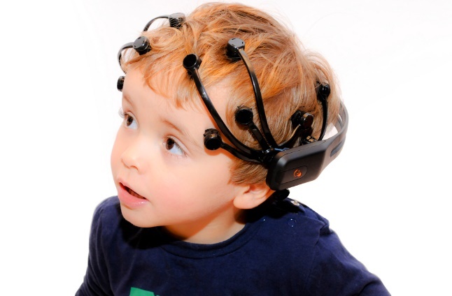
More recently the use of portable EEGs has become more prevalent, with the development of innovative technologies (see Fig. 1). Research has demonstrated that with use of portable headsets, the eye-state of a participant can be identified using the raw time-series recorded at different channels, rather than separating data into different frequency bands (Wang et al., 2014). Despite some concerns around the measurement capabilities of the headsets, the potential of portable devices in current and future research is recognized within the field (e.g. see (Xu and Zhong, 2018) for review in educational research). Portable EEGs are easier to implement than traditional EEGs and can be used with subjects ”in the field” or who may have difficulty sitting still (e.g. young children). Having online eye-state classification capabilities with this portable technology is an exciting step towards a dynamic resource in cognitive-neuroscientific research.

Figure 1. Example of portable EEG use with children.

The application of machine learning methods for the classification of EEG signals has been widely explored in the last two decades. Examples include methods for feature selection and optimization as in (Baig et al., 2017) and channel selection as in (Yang et al., 2012; Alotaiby et al., 2015), amongst others (see (Rösler and Suendermann, 2013) for a wide range of machine learning methods applied).

In previous work EEG signals have been used to classify eye-state relatively successfully using Incremental Attribute Learning (IAL) with extended timeseries (Wang et al., 2014). Epochs of ten seconds have also been adequate for identifying drowsiness from eyestate (Yeo et al., 2009). However, to be useful as an online classifier, a shorter snapshot of data must be used to identify eye-state rather than an extended time-series, to reduce calculation time and processing power. This is also important for identifying blinks, which typically last 100-400ms (Reddy and Behera, 2016). Levy (Levy, 1987) explored the effect of epoch length on signal analysis of the EEG and found that epochs as short as 2 seconds could be used for intraoperative EEG monitoring. For eye-state classification in particular, it has been demonstrated that a snapshot of EEG signal time-series in the alpha frequency range can be used to identify eye-state, rather than an extended time-series (Barry et al., 2007).

In this research, we provide experimental analysis for sample size reduction based on a method to capture signals in discrete EEG signal slices compared to longer EEG signal time-series. Additionally, we investigate the effect of possible signal redundancy on classification scores and computational performance. This will be investigated using the raw EEG data rather than splitting it into different frequency bands, therefore eliminating data preparation steps.

Results show that with both channel selection and sample reduction methods, we could accomplish comparable classification results with KNN, Support Vector Machines (Classifier: SVC), KNN and RF when run on the entire dataset containing signals from all channels. Additionally, outcomes suggest that significant computational speed-up could be achieved using a Mutual Information (MI) measure for EEG

2. Dataset

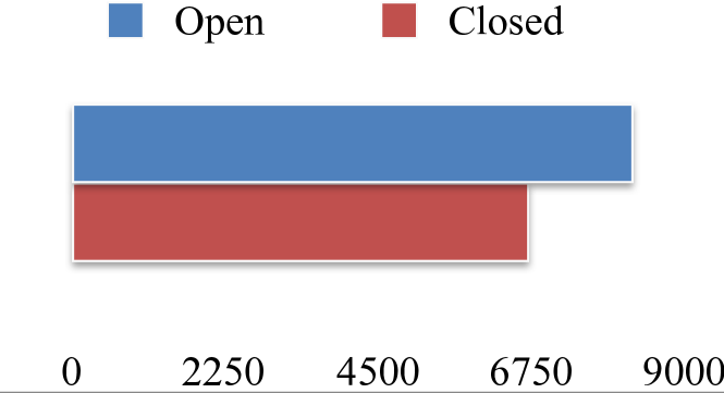
The data corpus explored in this work was collected and compiled by Roesler (Rösler and Suendermann, 2013), and provided for open access on UCI data repository(Irvine and Science, [n.d.]). The dataset comprises of raw electro-magnetic recordings taken from the scalp of one participant and information about eye-state (eyes open or closed) over the same time period. The participant was asked to relax, look forwards towards a camera and blink naturally, without restriction (Garrett et al., 2003). While looking toward the camera a video was recorded of the eye. Once recorded the video data was coded; binary labels were used to identify the two different eye-states; ’1’ for an ”eye-blink” and ’0’ for ”eye-open” state — the distribution of eye-states over the course of the recording in the dataset is shown in Fig. 2.

Figure 2. Eye-state distribution of the recorded observations.

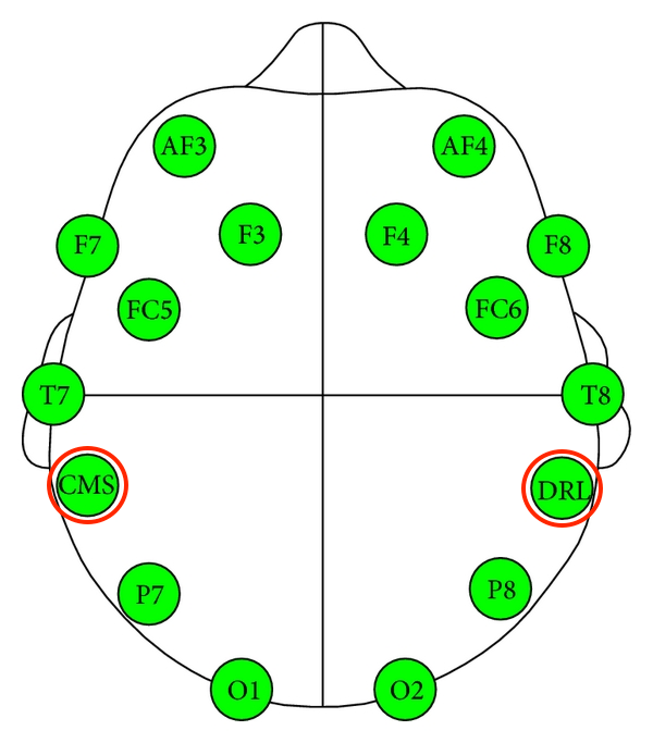
During this time, recordings were also taken at the scalp using the Emotiv EEG Neuroheadset, which measured the electro-magnetic signal at 14 electrode positions (see Fig. 3 - note that two electrode positions where excluded, as indicated in the figure). 14980 sequential timepoints (observations) were recorded from each of the 14 EEG channels (features), The recording took place over 117 seconds period (this is a rate of 128Hz) and measured signals were stored as floating-point values.

Figure 3. The 14 EEG channels compiled by Roesler(Rösler and Suendermann, 2013). Excluded channels are circled in red.

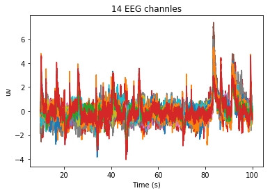
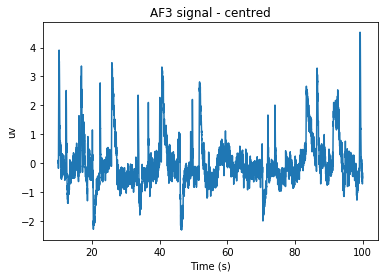
Initial exploration of the dataset indicated three outliers (value ¿ 10x the average recording) , which were removed. Observations were therefore reduced to 14977 at each electrode; each of these 14 timeseries represented the signal variability of an electrode over the experimental period. The timeseries were then normalised using zero centring (”de-meaning” applied) to explore the positive and negative deviation from their mean, as an indicator of signal similarity — centred signals are shown in Fig.4 . By eye, the timeseries show overall similarity across the different electrodes.

(a) 14 channel time-series

(b) 1 channel time-series

Figure 4. (a) Sliced window of the 14 EEG channel centered time-series- um is signal voltage. Signals show similarity across the EEG channels. (b) Only one channel (AF3) signal is shown.

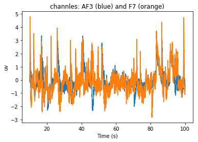
For example, a strong signal similarity can be observed when looking at the time-series of AF3 and F7 as in Fig. 5.

(a)

(b)

Figure 5. Signal time-series for AF3 and F7, (b) shows a smaller time-slot of the same time-series.

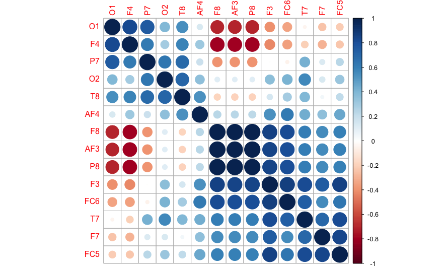
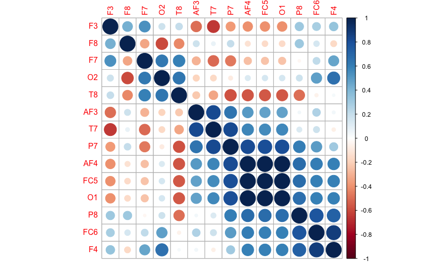
Similarities across the EEG timeseries are observable overall. Indeed, if we separate all EEG time-series relative to eye-state and cross-correlate, topological patterns in signal variability across the channels exist, see Fig. 6 (note that order of variables varies across the matrices to facilitate visualisation of possible similarities). The correlation between electrode signals is also seen to change during eyes-close state compared to eyes-open.

(a) eye-state=1

(b) eye-state=0

Figure 6. Correlation matrices for an ’eye-blink’ time-series in (a), and ’eye-open’ in (b). Hierarchical clustering (Hurley, 2004) is applied to cluster higher-correlated channels together. Note the difference of order in each matrix.

3. Methods and findings

Patterns between EEG channel signals relative to eye-state could be further explored by techniques from graph theory. Linear correlations between the time series $T_{i}(t_{k})$ and $T_{j}(t_{k})$ (the Pearson correlation coefficient $R_{ij}$) given by

(1) $$R_{ij}=\frac{{\sum\limits_{k=1}^{L}}T_{i}(t_{k})T_{j}(t_{k})}{\sqrt{(\sum\limits_{k=1}^{L}T^{2}_{i}(t_{k}))(\sum\limits_{k=1}^{L}T^{2}_{j}(t_{k}))}}$$

is widely used (Wilks, 2011), whereby strong linearity between two channels can be expressed as a link between two graph nodes. Having derived the correlation matrix $C$, a threshold $\tau$ is usually applied to define strong similarities between graph nodes as ‘links’. The adjacency matrix $A$ for the graph is then found by

(2) $$A_{ij}=A_{ji}=\Theta{(C_{ij}-\tau)}-\delta_{ij},$$

where $\Theta$ is the Heaviside function and $\delta$ is Kronecker delta. Graphs based on the two different eye-states have been constructed, considering different values for $\Theta$ — see Fig. 7.

(a) eye-open, $\Theta$ = 0.6

(b) eye-open, $\Theta$ = 0.7

(c) eye-open, $\Theta$ = 0.8

(d) eye-blink, $\Theta$ = 0.6

(e) eye-blink, $\Theta$ = 0.7

(f) eye-blink, $\Theta$ = 0.8

Figure 7. Different graphs constructed from 14 EEG channel time-series, relative to eye-state and a value for $\Theta$; strength of linear similarity.

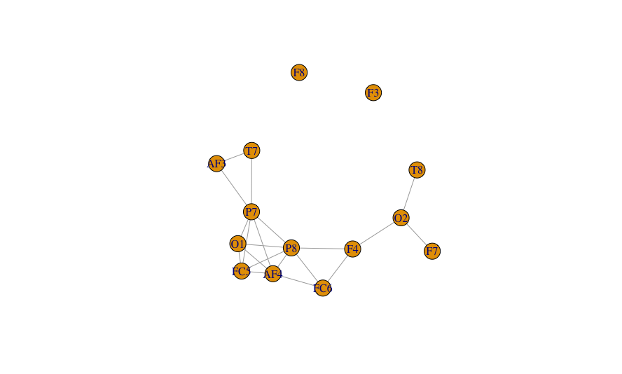
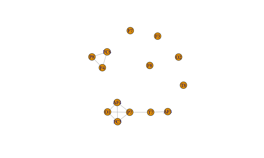
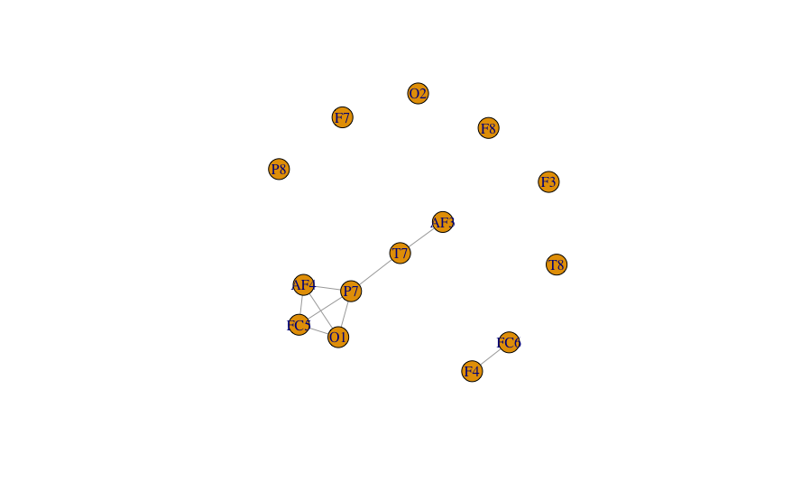
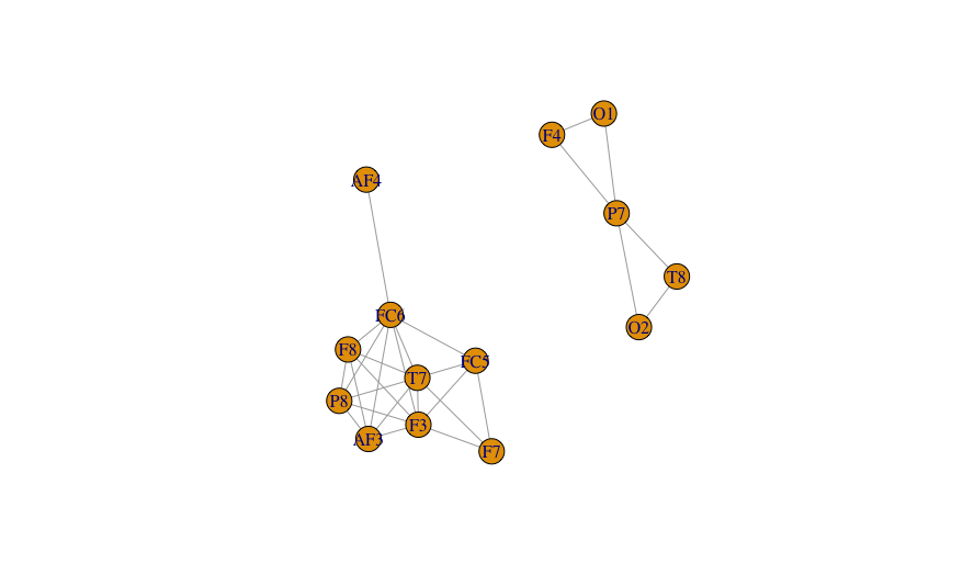
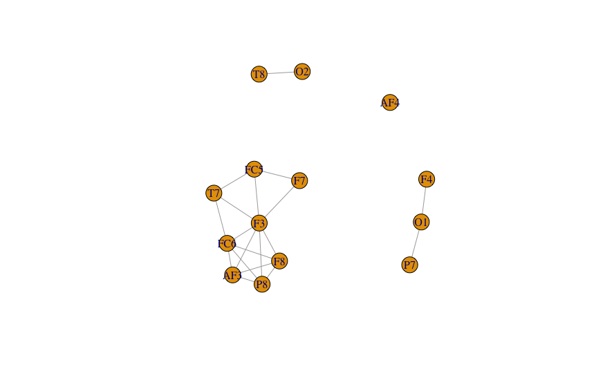
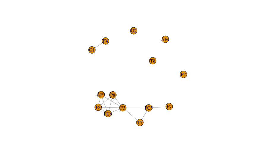
The constructed graphs (small, provided the number of channels) show a strong dissimilarity in topological structure between first set (eye-open signals) and the second (constructed from eye-blink signals). Studying metrics such as the average degree for nodes of both types of graphs can be used to quantify the topological similarity further.

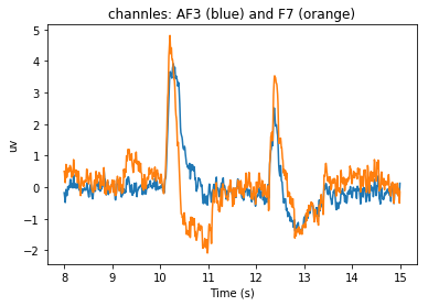
Based on observed similarities (linear similarity explored here), we argue that machine learning methods should provide comparable results if, on the one hand features’ space is reduced based on the relevance of features and their ’score’ of redundancy, and on another, the similarity between signals can be captured in shorter time-series of signals. To test both assumptions we sliced the provided time-series for all channels into time-windows of 3 seconds (384 timepoints, collected at a rate of 128Hz), containing a transition between eye-blink and eye-open and vice versa. — Fig 8 shows a time-series window of 7 seconds for demonstration purposes.

Figure 8. Example of F7 signal time-series window — window here is of 7 seconds. Light blue represent recordings in the closed-eye state and dark blue eyes-open.

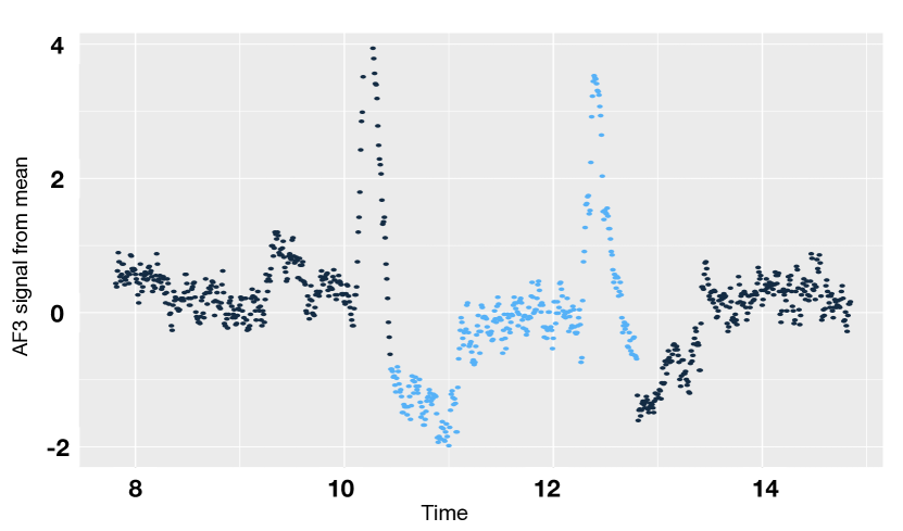
20 time-series slices (windows of 3s length each) were generated for each channel, resulting in the total number of observations reduced to 7,680. We then implemented a filtering approach based on mutual information ($M_{ij}$), given by

(3) $$M_{ij}=\sum\limits_{T_{i},T_{j}}{P_{ij}(T_{i},T_{j})\;\log\frac{P_{ij}(T_{i},T_{j})}{P_{i}(T_{i})P_{j}(T_{j})}}.$$

Here $P_{i}(T_{i})$ is the probability density function (PDF) of time series $T_{i}$, and $P_{ij}(T_{i},T_{j})$ is the joint PDF for $(T_{i},T_{j})$.

The minimum redundancy maximum relevance (mRMRe) algorithm (Battiti, 1994), as a filtering method, uses differences of $M_{ij}$ to compute the degree of dependency between multiple random variables. The method then sequentially compares the relevancy/redundancy balance of information between variables, providing scores for both their relevance and redundancy. The variable (channel time-series) selected at each step is the one with the highest score. A negative score indicates a redundancy final trade of information and a positive score indicates a relevancy final trade of information. The scoring results averaged for the 20 time-series slices is shown in Fig 9.

Figure 9. The variable selected at each step is the one with the highest scores (the variables are ordered in the plot). The scores at selection can thus be read from the diagonal.

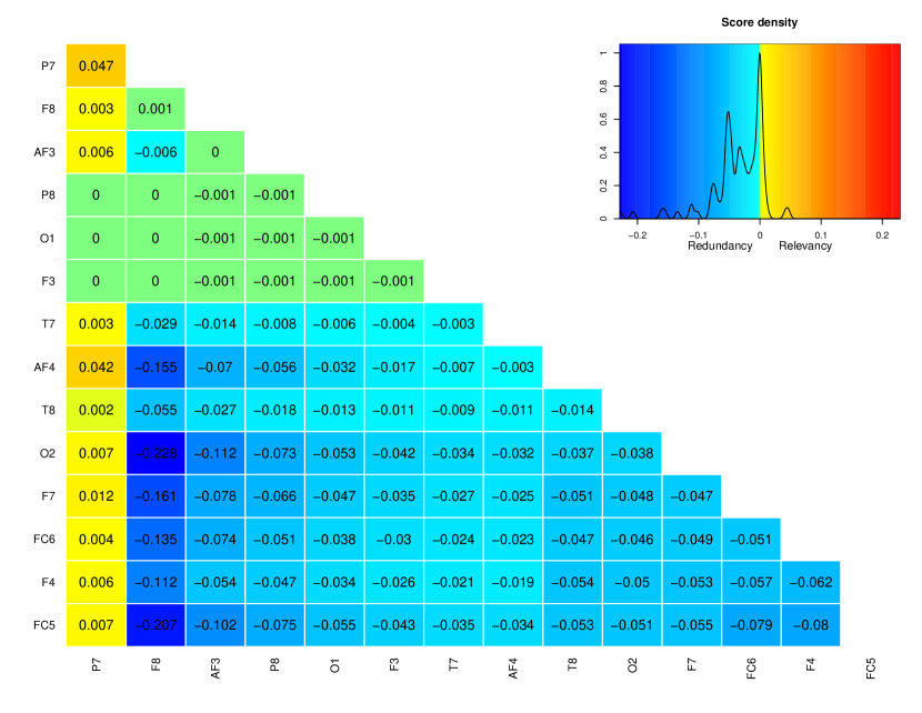
Accordingly we ran a series of experiments on a 3.2 GHz Intel Core i5 processor with 16 GB 1600 MHz DDR3 memory, which included a base run of different machine learning methods for classification; Nearest neighbors (KNN), Logistic Regression, Support Vector Machines classifier (SVC) and Random Forests (RF). The base run included the tuning of K for nearest neighbors and regularisation, using grid search methods, for SVC hyper-parameters (C=10, gamma=0.001) with radial basis function (rbf) kernel. RF is run with bootstrapping enabled and the number of selected features set to ’automatic’, in order to decrease variance amongst constructed member trees.

K-fold validation score of F1 metric was obtained over the entire dataset of 14977 time-series (117 seconds and sampling rate of 128Hz). Although F1 score’s value is not the main concern here, a comparison between classification methods’ accuracy can be found in (Rösler and Suendermann, 2013) and in (Reddy and Behera, 2016) for deep learning architectures’ performance. The resulting classification F1 Score and processing speed where then compared to those of 3 different experimental settings, for KNN, Logistic Regression, SVC and RF, which included:

• (A) 9 features from mRMRe analysis are selected from the available 14. Entire dataset of 14977 time-series is used to learn the classifiers. Accuracy and performance results compared to base run are shown in Table 1 below:

  Classifier	F1 Score gain	Speed-up gain
  $KNN$	-0.2	$2.1x$
  $LogReg$	-0.36	$2x$
  $SVC$	-0.3	$3x$
  $RF$	-0.5	$0.3x$

  Table 1. Accuracy and processing time comparison between base run and experiment A.

• (B) 9 features from mRMRe analysis are selected from the available 14. 7,680 observations (based reducing time-series to 20 sliced windows containing eye-state transition) used for learning. Accuracy and performance results compared to base run are shown in Table 2 below:

  Classifier	F1 Score gain	Speed-up gain
  $KNN$	-0.4	$4.3x$
  $LogReg$	-0.6	$2.5x$
  $SVC$	-0.7	$5.6x$
  $RF$	-0.7	$3x$

  Table 2. Accuracy and processing time comparison between base run and experiment B.

• (C) 14 features (no channel selection) on the 7,680 observations are used to learn a classifier. Accuracy and performance results compared to base run are shown in Table 3 below:

  Classifier	F1 Score gain	Speed-up gain
  $KNN$	-0.1	not observed
  $LogReg$	-0.17	$2.3x$
  $SVC$	-0.3	$1.9x$
  $RF$	-0.63	$3x$

  Table 3. Accuracy and processing time comparison between base run and experiment C.

The obtained results show some classification score penalty in most runs of the presented methods, generally, yet speed-up gain is promising. The accuracy score declines more as both feature reduction as well as data slicing method are applied together, however, processing speed-up gains are maximised. Further tuning to, namely, SVC is believed to show better scores by the application of this work’s methods, which we aim at focusing on for future developments. That said, the method introduced can be vastly useful for the analysis of higher-dimensional EEG/MEG signals which are typically characterised by the existence of both redundancy of information in their signals, and most importantly, noise.

4. Conclusions and further work

This paper presented a brief literature on the analysis of the electroencephalogram (EEG) signals and the application of their analysis. Information obtained by Emotiv headsets on subjects/humans include signal time-series from different electrodes, which typically exhibit variability, in response to events designed for a study of interest. The resolution of collected data as well as the quantity of time-series which could be obtained by such devices is, increasingly, producing both opportunities to gain further insights into brain functionality, and a challenge on the analysis side; accuracy and efficiency. In the presented work, we showed that efficiency could be improved with some (arguably marginal) penalty on a range of popular machine learning accuracy outcomes that are applied for the analysis of EEG data. The introduced method assumes that much of EEG signal information can be captured by (A) signals in a subset of EEG channels, which we filtered by the application of mRMRe technique and (B) signal information from discrete time-series slices (3secs) which contain signal (eye-state) transitions. Experimental results obtained show that both assumptions hold for the classification of eye-state from 14 EEG channels based on the dataset provided by Roesler, see Section 2.

When developing this work, results should be considered alongside deep neural network architectures which have shown low convergence times and may be applicable in real-time classification of eye-state (Reddy and Behera, 2016).

Slicing frequency and the number of features/channels to select have been done heuristically here, and therefore, based on these preliminary outcomes, we hope to validate the presented method and obtained outcomes on larger datasets, in future work. Also, we believe that more noticeable gains in learning efficiency should be possible for datasets of significantly higher-dimensional features’ spaces.

Code availability

Authors will provide link to code and dataset in camera-ready manuscript.

References

- (1)
- Alotaiby et al. (2015) Turky Alotaiby, Fathi E. Abd El-Samie, Saleh A. Alshebeili, and Ishtiaq Ahmad. 2015. A review of channel selection algorithms for EEG signal processing. EURASIP Journal on Advances in Signal Processing 2015, 1 (01 Aug 2015), 66. https://doi.org/10.1186/s13634-015-0251-9
- Baig et al. (2017) Muhammad Zeeshan Baig, Nauman Aslam, Hubert P.H. Shum, and Li Zhang. 2017. Differential evolution algorithm as a tool for optimal feature subset selection in motor imagery EEG. Expert Systems with Applications 90 (2017), 184 – 195. https://doi.org/10.1016/j.eswa.2017.07.033
- Barry et al. (2007) Robert J Barry, Adam R Clarke, Stuart J Johnstone, Christopher A Magee, and Jacqueline A Rushby. 2007. EEG differences between eyes-closed and eyes-open resting conditions. Clin Neurophysiol 118, 12 (Dec 2007), 2765–2773. https://doi.org/10.1016/j.clinph.2007.07.028
- Battiti (1994) R. Battiti. 1994. Using mutual information for selecting features in supervised neural net learning. IEEE Transactions on Neural Networks 5, 4 (1994), 537–550. https://doi.org/10.1109/72.298224
- Berger (1931) Hans Berger. 1931. Über das Elektrenkephalogramm des Menschen. Archiv für Psychiatrie und Nervenkrankheiten 94, 1 (01 Dec 1931), 16–60. https://doi.org/10.1007/BF01835097
- Boersma et al. (2011) Maria Boersma, Dirk J A Smit, Henrica M A de Bie, G Caroline M Van Baal, Dorret I Boomsma, Eco J C de Geus, Henriette A Delemarre-van de Waal, and Cornelis J Stam. 2011. Network analysis of resting state EEG in the developing young brain: structure comes with maturation. Hum Brain Mapp 32, 3 (Mar 2011), 413–425. https://doi.org/10.1002/hbm.21030
- Brovelli et al. (2002) Andrea Brovelli, Piero Paolo Battaglini, Jose Raul Naranjo, and Riccardo Budai. 2002. Medium-Range Oscillatory Network and the 20-Hz Sensorimotor Induced Potential. NeuroImage 16, 1 (2002), 130 – 141. https://doi.org/10.1006/nimg.2002.1058
- Ferrara and De Gennaro (2011) Michele Ferrara and Luigi De Gennaro. 2011. Going Local: Insights from EEG and Stereo-EEG Studies of the Human Sleep-Wake Cycle. Current topics in medicinal chemistry 11 (08 2011), 2423–37. https://doi.org/10.2174/156802611797470268
- Garrett et al. (2003) D. Garrett, D. A. Peterson, C. W. Anderson, and M. H. Thaut. 2003. Comparison of linear, nonlinear, and feature selection methods for EEG signal classification. IEEE Transactions on Neural Systems and Rehabilitation Engineering 11, 2 (2003), 141–144. https://doi.org/10.1109/TNSRE.2003.814441
- Haak et al. (2009) M Haak, S Bos, Sacha Panic, and Léon Rothkrantz. 2009. Detecting Stress using Eye Blinks during Game Playing. 10th International Conference on Intelligent Games and Simulation, GAME-ON 2009, 75–82.
- Hurley (2004) Catherine B Hurley. 2004. Clustering Visualizations of Multidimensional Data. Journal of Computational and Graphical Statistics 13, 4 (2004), 788–806. https://doi.org/10.1198/106186004X12425 arXiv:https://doi.org/10.1198/106186004X12425
- Irvine and Science ([n.d.]) School of Information Irvine, CA. University of California and Computer Science. [n.d.]. UCI Data Repository. https://archive.ics.uci.edu/ml/datasets/
- Levy (1987) W J Levy. 1987. Effect of epoch length on power spectrum analysis of the EEG. Anesthesiology 66, 4 (Apr 1987), 489–495.
- Reddy and Behera (2016) T. K. Reddy and L. Behera. 2016. Online Eye state recognition from EEG data using Deep architectures, In 2016 IEEE International Conference on Systems, Man, and Cybernetics (SMC). 2016 IEEE International Conference on Systems, Man, and Cybernetics (SMC), 000712–000717. https://doi.org/10.1109/SMC.2016.7844325
- Rösler and Suendermann (2013) Oliver Rösler and David Suendermann. 2013. A First Step towards Eye State Prediction Using EEG. In International Conference on Applied Informatics for Health and Life Sciences (AIHLS 13).
- Sandyk (1990) R Sandyk. 1990. The significance of eye blink rate in parkinsonism: a hypothesis. Int J Neurosci 51, 1-2 (Mar 1990), 99–103.
- Stam et al. (2005) C.J. Stam, T. Montez, B.F. Jones, S.A.R.B. Rombouts, Y. van der Made, Y.A.L. Pijnenburg, and Ph. Scheltens. 2005. Disturbed fluctuations of resting state EEG synchronization in Alzheimer’s disease. Clinical Neurophysiology 116, 3 (2005), 708–715. https://doi.org/10.1016/j.clinph.2004.09.022
- Vermani et al. (2015) Bhawna Vermani, Neha Hooda, and Neelesh Kumar. 2015. Parametric evaluation of EEG signal during Eyes Close and Eyes Open state. 1–5 pages. https://doi.org/10.1109/INDICON.2015.7443754
- Wang et al. (2014) T. Wang, S. U. Guan, K. L. Man, and T. O. Ting. 2014. Time Series Classification for EEG Eye State Identification Based on Incremental Attribute Learning, In 2014 International Symposium on Computer, Consumer and Control. 2014 International Symposium on Computer, Consumer and Control, 158–161. https://doi.org/10.1109/IS3C.2014.52
- Wilks (2011) Daniel S. Wilks. 2011. Statistical Methods in the Atmospheric Sciences. Elsevier. http://books.google.com/books?hl=en&lr=&id=IJuCVtQ0ySIC&oi=fnd&pg=PP2&dq=Statistical+Methods+in+the+Atmospheric+Sciences&ots=anFosWzIJ_&sig=kCqI0fmU8UjjV5ZtVlifGWGcSJc
- Xu and Zhong (2018) Jiahui Xu and Baichang Zhong. 2018. Review on portable EEG technology in educational research. Computers in Human Behavior 81 (2018), 340 – 349. https://doi.org/10.1016/j.chb.2017.12.037
- Yang et al. (2012) Jianhua Yang, Harsimrat Singh, Evor L. Hines, Friederike Schlaghecken, Daciana D. Iliescu, Mark S. Leeson, and Nigel G. Stocks. 2012. Channel selection and classification of electroencephalogram signals: An artificial neural network and genetic algorithm-based approach. Artificial Intelligence in Medicine 55, 2 (2012), 117 – 126. https://doi.org/10.1016/j.artmed.2012.02.001
- Yeo et al. (2009) Mervyn V.M. Yeo, Xiaoping Li, Kaiquan Shen, and Einar P.V. Wilder-Smith. 2009. Can SVM be used for automatic EEG detection of drowsiness during car driving? Safety Science 47, 1 (2009), 115 – 124. https://doi.org/10.1016/j.ssci.2008.01.007