Vacuum polarization instead of ”dark matter” in a galaxy

S.L. Cherkas ^a, V.L. Kalashnikov^b

^aInstitute for Nuclear Problems, Belarus State University

Minsk 220006, Belarus

Email: cherkas@inp.bsu.by

^b Department of Physics,

Norwegian University of Science and Technology,

Høgskoleringen 5, Realfagbygget, 7491, Trondheim, Norway

Email: vladimir.kalashnikov@ntnu.no

Submitted: August 30, 2022

We considered a vacuum polarization inside a galaxy in the eikonal approximation and found that two possible types of polarization exist. The first type is described by the equation of state $p=\rho/3$, similar to radiation. Using the conformally-unimodular metric allows constructing a nonsingular solution for this vacuum “substance”, if a compact astrophysical object exists in the galaxy’s center. As a result, a “dark” galactical halo appears that increases the rotation velocity of a test particle as a function of the distance from a galactic center. The second type of vacuum polarization has a more complicated equation of state. As a static physical effect, it produces renormalization of the gravitational constant, thus, causing no static halo. However, a nonstationary polarization of the second type, resulting from an exponential increase (or decrease) of the galactic nuclei mass with time in some hypothetical time-dependent process, produces a gravitational potential looking like a dark matter halo.

I Introduction

Among the various issues of combining general relativity (GR) and the quantum mechanics, one encounters the problems of vacuum energy and black holes.

The first problem is to explain why enormous zero-point vacuum energy density $\rho_{v}\sim k_{max}^{4}$ (here $k_{max}$ is the UV energy scale of quantum field theory associated with a hard 3-momentum cutoff of the order of the Planck mass $M_{p}$) does not influence a universe expansion (e.g., see [1, 2, 3] and references herein). The second problem is associated with the loss of unitarity and information inside of the black hole horizon (e.g., see [4, 5] and references therein), that prevents the definition of a pure quantum state.

On the other hand, the basis of GR is a notion of manifold [6], i.e., a metric space, which could be covered by coordinate maps. When a concrete space-time possessing some symmetry is considered, one aims to introduce a system of coordinates allowing maximal covering of this particular manifold. For instance, the Schwarzschild solution only describes the region outside the horizon, and one has to introduce the Kruscal coordinates to cover the complete domain [7]. Nevertheless, one could admit an opposite view: restricting the manifold by sewing all the black hole horizons by some coordinate transformation. This approach is similar to a case when a man finds a hole in his trousers at a knee. In such a case, he steps back a little from the hole border and then subtends it into a node with the help of sewing.

It is allowed using the conformally-unimodular (CUM) metric [8], where an ultra-compact black hole-like astrophysical object appears as a nonsingular ball named “eicheons” [9]. Besides, the vacuum energy problem could be partially solved in the CUM metric if one builds a gravity theory admitting an arbitrary choice of the energy density level [8]. That is possible because the equations for evolution of the Hamiltonian $\mathcal{H}$ and the momentum constraints $\mathcal{P}$ admit not only the trivial solution $\mathcal{P}=0$, $\mathcal{H}=0$, but also $\mathcal{P}=0$, $\mathcal{H}=const$. The constant compensates for the main part of the vacuum energy density proportional to the Planck mass in the fourth degree [8, 10]. Residual energy density, remaining after omitting the main part of the vacuum energy density, is some kind of dark energy and results in a cosmological picture containing a period of linear evolution in cosmic time [11, 10] followed by late accelerated expansion.

Both dark energy and dark matter (DM) are unknown “substances” appearing in modern cosmology and astrophysics [12, 13, 14]. DM appears not only in cosmological scales but also at galaxy scales. The lowest scale at which there is evidence for DM is of $\approx$ kpc [15, 16]. Dark energy is associated with vacuum energy, whereas DM is expected to be some kind of a non-baryonic matter weakly interacting with the known particles of the standard model [17, 18, 19]. Nevertheless, there are attempts to explain the DM by a DM-like behavior of vacuum energy [20], or a vacuum polarization induced by the gravitational field. Heuristic models of vacuum polarization like [21, 22, 23, 24, 25], which would demand dipolar fluid [26], anti-gravitation [27] or hydrodynamical phenomena in a vacuum treated as hypothetical (super-)fluid [28, 29, 30], are of interest.

The conventional renormalization procedure of the quantum field theory applied to vacuum energy near a massive object [31, 32, 33, 34, 35, 36], leads to modification of the gravitational potential only at small distances of the order of gravitational radius that are unobservable with current technologies. That is, the renormalization excludes the manifestation of micro-scale phenomena on the macro-scales (nevertheless, see [20]). This conclusion assumes the general covariance of the mean vacuum value of stress-energy tensor $<0|T_{\mu\nu}|0>$ on a curved background. However, the vacuum state $|0>$, invariant relatively general transformation of coordinates does not exist [37]. That raises a question: is it reasonable to demand the covariance of $<0|T_{\mu\nu}|0>$ in the absence of invariant $|0>$? If invariance violation, which implies the existence of “æther”, takes place, then, like condensed-matter physics, DM still could be treated as an emergent phenomenon produced by vacuum polarization.

The outline of this paper is as follows. In Section II, we argue the necessity of considering a vacuum polarization from a cosmological point of view and explain that the CUM metric is needed to omit the main part of vacuum energy. Section III contains a perturbation formalism in the CUM metric, which is required to introduce a vacuum polarization as some media, i.e., “æther”. The eikonal approximation is used in Section IV to obtain the vacuum energy density and pressure of a quantum scalar field by summating the contributions from the distorted virtual plane waves. The expression for a vacuum equation of state is obtained. In Section V, the $F$-type vacuum polarization, possessing a radiation equation of state, is used in the Tolman-Volkov-Oppenheimer (TOV) equations for two substances. This type of vacuum polarization results in a dark halo if eicheon is situated in the galactic center. In Section VI, the $\Phi$-type of vacuum polarization is considered. This type of polarization leads to the renormalization of the gravitational constant in the stationary case. But it can contribute to the DM halo for the nonstationary processes. In Conclusion, we summarize the consequences of two types of vacuum polarization for galaxies. In Appendix, we consider the static and empty universe to demonstrate an example of an exact solution for the system of perturbations, taking into account the $F$-type vacuum polarization.

II A spatially uniform universe in the CUM metric

II.1 CUM metric in the five vectors theory of gravity

We based our analysis on using the CUM metric, which is the foundation of the so-called five vectors theory (FVT) [8]. In the course of this analysis, we will use the particular cases of the CUM metric appropriate to the physics considered.

A general class of CUM metrics is defined as [8]

$$ds^{2}\equiv g_{\mu\nu}dx^{\mu}dx^{\nu}=a^{2}\left(1-\partial_{m}P^{m}\right)^{2}d\eta^{2}-\gamma_{ij}(dx^{i}+N^{i}d\eta)(dx^{j}+N^{j}d\eta),$$ (1)

where $x^{\mu}=\{\eta,\bm{x}\}$, $\gamma_{ij}$ is a spatial metric, $a=\gamma^{1/6}$ is a locally defined scale factor, and $\gamma=\det\gamma_{ij}$, $\eta$ is a conformal time connected with a cosmic time $t$ through $dt=a(\eta,\bm{x})d\eta$. The spatial part of the interval (1) looks as

$$dl^{2}\equiv\gamma_{ij}dx^{i}dx^{j}=a^{2}(\eta,\bm{x})\tilde{\gamma}_{ij}dx^{i}dx^{j},$$ (2)

where $\tilde{\gamma}_{ij}=\gamma_{ij}/a^{2}$ is a matrix with the unit determinant. The interval (1) is similar formally to the ADM one [38], but the lapse function is taken in the form of $a(1-\partial_{m}P^{m})$, where $P^{m}$ is a three-dimensional vector, and $\partial_{m}$ is a conventional partial derivative. In the gravity theory admitting arbitrary choice of the energy density level [8], there are the Lagrange multipliers $\bm{P}$, the shift function $\bm{N}$, and three triads $\bm{e}^{a}$ to parameterize the spatial metric $\gamma_{ij}=e^{a}_{i}e^{a}_{j}$. Such model was named the FVT of gravity [8]. In contrast to GR, where the lapse and shift functions are arbitrary, the restrictions $\partial_{n}(\partial_{m}N^{m})=0$ and $\partial_{n}(\partial_{m}P^{m})=0$ arise in FVT. The Hamiltonian $\mathcal{H}$ and momentum $\mathcal{P}_{i}$ constraints in the particular gauge $P^{i}=0$, $N^{i}=0$ obey the constraint evolution equations [8]:

$$\partial_{\eta}{\mathcal{H}}=\partial_{i}\left(\tilde{\gamma}^{ij}\mathcal{P}_{j}\right),$$ (3)

$$\partial_{\eta}{\mathcal{P}_{i}}=\frac{1}{3}\partial_{i}{\mathcal{H}},$$ (4)

which admits adding some constant to ${\mathcal{H}}$. In the FVT frame, it is not necessary that $\mathcal{H}=0$, but $\mathcal{H}=const$ is also allowed. The particular cases of the CUM metric corresponding to the Bianchi I model and the spherically symmetric space-time were analyzed in [39, 40].

II.2 Uniform, isotropic and flat universe

Let us consider a particular case of (1)

$$ds^{2}=a(\eta)^{2}(d\eta^{2}-d\bm{x}^{2})$$ (5)

corresponding to a spatially uniform, isotropic and flat universe, where the Friedmann equations take the form [11, 41, 42]:

$$M_{p}^{-2}e^{4\alpha}\rho-\frac{1}{2}e^{2\alpha}\alpha^{\prime 2}=const,$$ (6)

$$\alpha^{\prime\prime}+\alpha^{\prime 2}=M_{p}^{-2}e^{2\alpha}(\rho-3p).$$ (7)

Here $\alpha(\eta)=\log a(\eta)$, the prime denotes the derivative in respect to the conformal time. We use the system of units $\hbar=c=1$ and the reduced Planck mass $M_{p}=\sqrt{\frac{3}{4\pi G}}$ (in physical units $M_{p}=\sqrt{\frac{3\hbar c}{4\pi G}}$ ). According to FVT [8], the first Friedmann equation (6) is satisfied up to some constant, and the main parts of the vacuum energy density and pressure

$$\rho_{v}\approx(N_{boson}-N_{ferm})\frac{k_{max}^{4}}{16\pi^{2}a^{4}},$$ (8)

$$p_{v}=\frac{1}{3}\rho_{v}$$ (9)

do not contribute to the universe expansion because the constant in (6) compensates the vacuum energy density, whereas there is no vacuum contribution in Eq. (7) by virtue of the equation of state (9).

Bosons and fermions contribute with opposite signs into a vacuum energy density (8) [43, 44]. Here, we do not consider the supersymmetry hypotheses $N_{boson}-N_{ferm}$ due to the absence of evidence for supersymmetric partners to date [45].

For the mass contributions of particles and condensates, we imply the Pauli sum rules [44, 46]. These rules are not fulfilled at this moment due to the incompleteness of the standard model. Nevertheless, one may hope they will be satisfied after possible discoveries beyond the standard model.

Other contributors to the vacuum energy density are the terms depending on the derivatives of the universe expansion rate [41, 46, 42, 10]. They have the correct order of magnitude $\rho_{v}\sim M_{p}^{2}H^{2}$, where $H$ is the Hubble constant, and explain the accelerated expansion of the universe driven by the residual energy density and pressure [41, 46, 42, 10]:

$$\rho_{v}=\frac{a^{\prime 2}}{2a^{6}}M_{p}^{2}(2+N_{sc}){\mathcal{S}}_{0},~{}~{}~{}~{}p_{v}=\frac{M_{p}^{2}(2+N_{sc}){\mathcal{S}}_{0}}{a^{6}}\left(\frac{1}{2}a^{\prime 2}-\frac{1}{3}a^{\prime\prime}a\right),$$ (10)

where ${\mathcal{S}}_{0}=\frac{k_{max}^{2}}{8\pi^{2}M_{p}^{2}}.$ Eqs. (10) include the number of minimally coupled scalar fields $N_{sc}$ plus two degrees of freedom of the gravitational waves [41]. The massless fermions and photons do not contribute to (10) [41].

According to (10), the accelerated expansion of universe allows finding a value of the momentum UV cut-off

$$k_{max}\approx\frac{12M_{p}}{\sqrt{2+N_{sc}}}$$ (11)

from the measured value of the universe deceleration parameter and other cosmological observations [41, 10]. It should be noted that the UV cut-off of the 3-momentums $k_{max}$ in (8) and hereafter also reflects the diffeomorphism symmetry violation (e.g., see [47, 48, 49, 50, 51, 52] and references herein).

III Perturbations of a uniform background in the CUM metric

In this section, the scalar perturbations of the CUM metric (1) are considered [53]:

$$ds^{2}=a(\eta,\bm{x})^{2}\left(d\eta^{2}-\left(\left(1+\frac{1}{3}\sum_{m=1}^{3}\partial_{m}^{2}F(\eta,\bm{x})\right)\delta_{ij}-\partial_{i}\partial_{j}F(\eta,\bm{x})\right)dx^{i}dx^{j}\right).$$ (12)

Here the perturbations of the locally defined scale factor are expressed through a gravitational potential $\Phi$:

$$a(\eta,\bm{x})=e^{\alpha(\eta,\bm{x})}\approx e^{\alpha(\eta)}(1+\Phi(\eta,\bm{x})).$$ (13)

A stress-energy tensor can be written in the hydrodynamic approximation

$$T_{\mu\nu}=(p+\rho)u_{\mu}u_{\nu}-p\,g_{\mu\nu}.$$ (14)

The perturbations of the energy density $\rho(\eta,\bm{x})=\rho(\eta)+\delta\rho(\eta,\bm{x})$ and pressure $p(\eta,\bm{x})=p(\eta)+\delta p(\eta,\bm{x})$ are considered around spatially uniform values.

Let us introduce new variables

$$\wp(\eta,\bm{x})=a^{4}(\eta,\bm{x})\rho(\eta,\bm{x}),$$ (15)

$$\Pi(\eta,\bm{x})=a^{4}(\eta,\bm{x})p(\eta,\bm{x})$$ (16)

for reasons which will be explained below. The perturbations of (15), (16) around the uniform values can be written now as $\wp(\eta,\bm{x})=e^{4\alpha(\eta)}\rho(\eta)+\delta\wp(\eta,\bm{x})$, $\Pi(\eta,\bm{x})=e^{4\alpha(\eta)}p(\eta)+\delta\Pi(\eta,\bm{x})$. The 4-velocity $u$ is represented in the form of

$$u^{\mu}=e^{-\alpha(\eta)}\{1,\bm{\nabla}\frac{v(\eta,\bm{x})}{\rho(\eta)+p(\eta)}\}\approx\{e^{-\alpha(\eta)}(1-\Phi(\eta,\bm{x})),e^{3\alpha(\eta)}\bm{\nabla}\frac{v(\eta,\bm{x})}{\wp(\eta)+\Pi(\eta)}\},$$ (17)

where $v(\eta,\bm{x})$ is a scalar function. Expanding all perturbations into the Fourier series $\delta\wp(\eta,\bm{x})=\sum_{\bm{k}}\delta\wp_{\bm{k}}(\eta)e^{i\bm{k}\bm{x}}...$ etc. results in the equations for the perturbations:

$$-6\Phi_{\bm{k}}^{\prime}+6\alpha^{\prime}\Phi_{\bm{k}}+k^{2}F_{\bm{k}}^{\prime}+\frac{18}{M_{p}^{2}}e^{-2\alpha}\sum_{i}v_{\bm{k}i}=0,$$ (18)

$$-18\alpha^{\prime}\Phi_{\bm{k}}^{\prime}-6(k^{2}+3\alpha^{\prime 2})\Phi_{\bm{k}}+k^{4}F_{\bm{k}}+\frac{18}{M_{p}^{2}}e^{-2\alpha}\sum_{i}\delta\wp_{\bm{k}i}\,=0,$$ (19)

$$-12\Phi_{\bm{k}}-3(F_{\bm{k}}^{\prime\prime}+2\alpha^{\prime}F_{\bm{k}}^{\prime})+k^{2}F_{\bm{k}}=0,$$ (20)

$$-9(\Phi_{\bm{k}}^{\prime\prime}+2\alpha^{\prime}\Phi_{\bm{k}}^{\prime})-9(2\alpha^{\prime\prime}+2\alpha^{\prime 2}+k^{2})\Phi_{\bm{k}}+k^{4}F_{\bm{k}}-\frac{9}{M_{p}^{2}}e^{-2\alpha}\left(\sum_{i}3\delta\Pi_{\bm{k}i}-\delta\wp_{\bm{k}i}\right)=0,$$ (21)

where the index $i$ denoting the kind of substance has been introduced. It is remarkable that, as a result of the choice of the variables (15), (16), (17), the unperturbed values $\rho$ and $p$ do not appear in the system (18)-(21). That allows us to avoid the influence of the large uniform energy density and pressure (8), (9) on the evolution of perturbation. Eqs. (18), (19) are consequences of the Hamiltonian and momentum constraints, while Eqs. (20), (21) are equations of motion. For consistency of the constraints with the equations of motion, every kind of fluid has to satisfy the continuity and Euler equations:

$$\alpha^{\prime}(\delta\wp_{\bm{k}i}-3\delta\Pi_{\bm{k}i})-(3\Pi_{i}-\wp_{i})(\Phi_{\bm{k}}^{\prime}-4\Phi_{\bm{k}}\alpha^{\prime})+4\wp_{i}^{\prime}\Phi_{\bm{k}}-\delta\wp_{\bm{k}i}^{\prime}+k^{2}v_{\bm{k}i}=0,$$ (22)

$$\Phi_{\bm{k}}(\wp_{i}-3\Pi_{i})+\delta\Pi_{\bm{k}i}+v_{\bm{k}i}^{\prime}=0.$$ (23)

The equations (18)-(23) have the same form as in GR, but for the consistency of Hamiltonian and momentum constraints (18), (19) with the equations of motions (20)-(23), it is sufficient for the first Friedmann equation (6) to be valid up to some constant. Namely, for such consistency, it is necessary that the differentiation of constraints with the subsequent substitution of the second time derivatives from the equations of motion (7), (20)-(23) lead to identical equalities. This consistency is a feature of using the CUM metric, in particular, and the FVT theory, in general. In any other metrics different from CUM (that is, in a frame of GR), the first Friedmann equation (6) with the $const=0$ in the right hand side is needed for consistency of the constraints and the equations of motion.

IV Vacuum as a medium: the eikonal approximation for quantum fields

Generally, a vacuum could also be considered as some fluid (e.g., see [28, 29, 30]), i.e., “æther” [54], but with some stochastic properties along with its elastic ones [46, 42, 55]. Here we are interested in its elastic properties only. In Refs. [46, 42], the speed of sound for the scalar waves of vacuum polarization $c_{s}^{2}=\frac{p_{v}^{\prime}(\eta)}{\rho_{v}^{\prime}(\eta)}$ was introduced, where $p_{v}$ and $\rho_{v}$ are given by (10). That is only heuristic conjecture.

Here the actual calculations of the vacuum density and pressure on the curved background are performed in the eikonal approximation. The last one has a very transparent background. In the Minkowski’s space-time, the virtual plane waves penetrate space-time and, to obtain a vacuum energy density, we must summarize the contributions of every wave. In the curved space-time, it is necessary to summarize the contributions of the distorted waves to obtain the spatially non-uniform energy density and pressure. It should be mentioned that the eikonal approximation was successfully used in high energy physics [56] and even in gravity [57], where the small-angle scattering amplitude of two massive particles were calculated in all orders on gravitational constant $G$.

A massless scalar field in the external gravitational field obeys the equation

$$\frac{1}{\sqrt{-g}}\partial_{\mu}\left(\sqrt{-g}g^{\mu\nu}\partial_{\nu}\right)\phi=0.$$ (24)

Using the gauge $\bm{N}=0$, $\bm{P}=0$ in (1) reduces the CUM metric to

$$ds^{2}=a^{2}(d\eta^{2}-\tilde{\gamma}_{ij}dx^{i}dx^{j}),$$ (25)

so that Eq. (24) takes the form

$$\phi^{\prime\prime}+2\frac{a^{\prime}}{a}\phi^{\prime}-\frac{1}{a^{2}}\partial_{i}\left(a^{2}\tilde{\gamma}^{ij}\partial_{j}\right)\phi=0.$$ (26)

That leads to

$$\chi^{\prime\prime}-\chi\frac{a^{\prime\prime}}{a}-\tilde{\gamma}^{ij}\partial_{i}\partial_{j}\chi\ -\partial_{i}\tilde{\gamma}^{ij}\partial_{j}\,\chi+\frac{\chi}{a}\left(\tilde{\gamma}^{ij}\partial_{i}\partial_{j}a+\partial_{j}a\partial_{i}\tilde{\gamma}^{ij}\right)=0$$ (27)

after the change of variables $\phi=\chi/a$. Further, in the terms of the metric perturbations $\Phi$ and $F$, we come to

$$\chi^{\prime\prime}-\Delta\chi+\hat{V}\chi=0,$$ (28)

where a “potential” operator $\hat{V}$ has the form

$$\hat{V}=-\alpha^{\prime\prime}-\alpha^{\prime 2}-2\alpha^{\prime}\Phi^{\prime}-\Phi^{\prime\prime}+\Delta\Phi+\frac{1}{3}\Delta F\,\Delta-\frac{\partial^{2}F}{\partial x^{j}\partial x^{i}}\frac{\partial^{2}}{\partial x^{j}\partial x^{i}}-\frac{2}{3}(\bm{\nabla}(\Delta F))\cdot\bm{\nabla}~{}~{}.~{}~{}$$ (29)

A quantization of the scalar field in terms of creation and annihilation operators implies [37]

$$\hat{\chi}(\eta,\bm{x})=\sum_{\bm{k}}u_{\bm{k}}(\eta,\bm{x})\hat{\mbox{a}}_{\bm{k}}+u_{\bm{k}}^{*}(\eta,\bm{x})\hat{\mbox{a}}_{\bm{k}}^{+},$$ (30)

where the function $u_{\bm{k}}$ satisfies Eq. (27), and the orthogonality condition is [37]

$$\int(u_{\bm{k}}\partial_{\eta}u_{\bm{q}}^{*}-u_{\bm{k}}^{*}\partial_{\eta}u_{\bm{q}})d^{3}\bm{x}=i\delta_{\bm{k}\bm{q}}.$$ (31)

Solution of Eqs. (27), (29) for the functions $u_{\bm{k}}$ can be written in the eikonal approximation

$$u_{\bm{k}}(\eta,\bm{x})=\frac{1}{\sqrt{2k}}\exp\left(-i\eta k+i\bm{k}\bm{x}-i\Theta_{\bm{k}}(\eta,\bm{x})\right),$$ (32)

which leads to the equation for the eikonal function

$$2k\Theta_{\bm{k}}^{\prime}+\left(2k_{m}\tilde{\gamma}^{mj}-i\partial_{m}\tilde{\gamma}^{mj}\right)\partial_{j}\Theta_{\bm{k}}+\frac{1}{a}\bigl{(}a^{\prime\prime}-\tilde{\gamma}^{ij}\partial_{i}\partial_{j}a-\partial_{j}a\partial_{i}\tilde{\gamma}^{ij}\bigr{)}+i\,k_{j}\partial_{m}\tilde{h}^{mj}-k_{m}k_{j}\tilde{h}^{mj}=0,$$ (33)

and, according to Eqs. (12), (13), is written in the terms of the metric perturbations $\Phi(\eta,\bm{x})$, $F(\eta,\bm{x})$:

$$k\Theta_{\bm{k}}^{\prime}+\bm{k}\bm{\nabla}\Theta_{\bm{k}}(\eta,\bm{x})=\frac{1}{2}V_{\bm{k}},$$ (34)

where

$$V_{\bm{k}}(\eta,\bm{x})=-2\alpha^{\prime}\Phi^{\prime}-\Phi^{\prime\prime}+\Delta\Phi+k_{i}k_{j}\partial_{i}\partial_{j}F-\frac{k^{2}}{3}\Delta F.$$ (35)

A solution of (34) can be obtained in the form

$$\Theta_{\bm{k}}(\eta,\bm{x})=\frac{1}{2k}\int_{\eta_{0}}^{\eta}\,V_{\bm{k}}\left(\tau,\bm{x}+\frac{\bm{k}}{k}(\tau-\eta)\right)d\tau,$$ (36)

where the lower integration limit $\eta_{0}$ depends on the cosmological model. In particular, it could be $0$ or $-\infty$. The mean value of the stress-energy tensor of a massless scalar field

$$\hat{T}_{\mu\nu}=\partial_{\mu}\,{\hat{\phi}}\partial_{\nu}{\hat{\phi}}-\frac{1}{2}g_{\mu\nu}g^{\alpha\beta}\partial_{\alpha}\,{\hat{\phi}}\partial_{\beta}\hat{\phi}$$ (37)

can be averaged over the vacuum state and compared with the hydrodynamic expression (14). That gives

$$\delta\wp(\eta,\bm{x})=e^{2\alpha(\eta)}<0|\frac{\hat{\phi}^{\prime 2}}{2}+\frac{(\bm{\nabla}\hat{\phi})^{2}}{2}|0>\approx\frac{1}{2}\sum_{\bm{k}}\frac{\alpha^{\prime}\Phi^{\prime}}{k}+\Theta_{\bm{k}}^{\prime}-\frac{\bm{k}\bm{\nabla}\Theta_{\bm{k}}}{k},$$ (38)

$$\delta\Pi(\eta,\bm{x})=e^{2\alpha(\eta)}<0|\frac{\hat{\phi}^{\prime 2}}{2}-\frac{(\bm{\nabla}\hat{\phi})^{2}}{6}|0>\approx\frac{1}{2}\sum_{\bm{k}}\frac{\alpha^{\prime}\Phi^{\prime}}{k}+\Theta_{\bm{k}}^{\prime}+\frac{\bm{k}\bm{\nabla}\Theta_{\bm{k}}}{3k},$$ (39)

$$\bm{\nabla}v=-e^{2\alpha(\eta)}<0|\hat{\phi}^{\prime}\bm{\nabla}{\hat{\phi}}|0>\approx\sum_{\bm{k}}\frac{\bm{k}\,\Theta^{\prime}_{\bm{k}}}{k}-\bm{\nabla}\Theta_{\bm{k}}-\frac{\alpha^{\prime}\bm{\nabla}\Phi}{k},$$ (40)

where only spatially non-uniform parts of the vacuum averages are implied in the second equalities on the right-hand side of (38), (39) and (40). The last depends on the metric perturbations $F(\eta,\bm{x})$ and $\Phi(\eta,\bm{x})$ contained in Eqs. (12), (13). The final equalities in (38), (39) and (40) result from calculations in the eikonal approximation (32).

Considering the quantity $\delta\wp(\eta,\bm{x})-3\delta\Pi(\eta,\bm{x})$ and using equations (34) and (35) result in

$$\delta\wp(\eta,\bm{x})-3\delta\Pi(\eta,\bm{x})=-\sum_{\bm{k}}\frac{\bm{k}\bm{\nabla}\Theta_{\bm{k}}}{k}+\Theta_{\bm{k}}^{\prime}+\frac{\alpha^{\prime}\Phi^{\prime}}{k}=~{}~{}~{}~{}~{}~{}~{}~{}~{}~{}~{}~{}~{}~{}~{}~{}~{}~{}~{}~{}~{}~{}~{}~{}~{}~{}~{}~{}~{}~{}~{}~{}~{}~{}~{}~{}~{}~{}~{}~{}~{}~{}~{}~{}~{}~{}~{}~{}~{}~{}~{}~{}~{}~{}~{}~{}$$

$$-\sum_{\bm{k}}\frac{1}{2k}V_{\bm{k}}+\frac{\alpha^{\prime}\Phi^{\prime}}{k}=\sum_{\bm{k}}\frac{1}{2k}\left(\Phi^{\prime\prime}-\Delta\Phi-k_{i}k_{j}\partial_{i}\partial_{j}F+\frac{k^{2}}{3}\Delta F\right)=\frac{N_{sc}}{8\pi^{2}}k_{max}^{2}(\Phi^{\prime\prime}-\Delta\Phi),$$ (41)

where summation has been changed by integration $\sum_{\bm{k}}\rightarrow\int d^{3}\bm{k}/(2\pi)^{3}$ and it is taken into account that

$\int_{k<k_{max}}\frac{1}{2k}\left(k_{i}k_{j}-\frac{k^{2}}{3}\delta_{ij}\right)d^{3}\bm{k}=0$. The number $N_{sc}$ of the scalar fields minimally coupled with gravity has been introduced also in (10).

In consequence of Eq. (41), two types of spatially nonuniform vacuum polarization exist. Namely, the $F$-polarization has a radiation-type equation of state

$$\delta\Pi_{vF}(\eta,\bm{x})=\frac{1}{3}\delta\wp_{vF}(\eta,\bm{x}),$$ (42)

whereas the $\Phi$-polarization has an equation of state

$$\delta\Pi_{v\Phi}(\eta,\bm{x})=\frac{1}{3}\delta\wp_{v\Phi}(\eta,\bm{x})-\frac{N_{sc}}{24\pi^{2}}k_{max}^{2}(\Phi^{\prime\prime}-\Delta\Phi).$$ (43)

Both types of spatially nonuniform vacuum polarizations correspond to the uniform component of (8), (9), whereas the uniform polarization given by (10) has no non-uniform counterpart with an accuracy of our consideration, i.e., in the second-order on derivatives. It must be emphasized that it is easy to obtain the equation of state (9) for a spatially uniform main part of the vacuum energy density, but it is not so trivial to do that for a spatially non-uniform vacuum energy density.

In principle, the system (18,19,20,21,22,23,42,43) is a fundamental system allowing to consider a broad range of cosmological and astrophysical phenomena including CMB and BAO. However below, we restrict ourselves to a galactic DM, which scales from kpc to Mpc.

V Galactic DM as a $F$-vacuum polarization

As it was shown in the section IV, the $F$-component of vacuum polarization has the equation of state analogous to radiation (see Eq. 9). In this sense, it is similar to the uniform part of vacuum energy density in Eq. (8).

At the same time, it is difficult to determine the concrete value of the nonuniform vacuum energy density because, according to (38), it contains an eikonal function $\Theta_{\bm{k}}$, which is determined by the integral (36). For instance, one has $\Theta_{\bm{k}}(\eta,\bm{r})=\sum_{\bm{q}}\tilde{\Theta}_{\bm{k},\bm{q}}(\eta)e^{i\bm{q}\bm{r}}$ from (35),(36) and

$$\tilde{\Theta}_{\bm{k},\bm{q}}(\eta)=\frac{1}{k}\left(\frac{1}{3}k^{2}q^{2}-(\bm{q}\bm{k})^{2}\right)\int_{\eta_{0}}^{\eta}F_{\bm{q}}(\tau)e^{i\bm{k}\bm{q}(\tau-\eta)/k}d\tau.$$ (44)

Calculation of the integral (44) requires one to know the full evolution history of $F_{\bm{q}}(\tau)$. It is simpler to use only the fact that the F-contribution to the vacuum polarization has the equation of state

$$p_{vF}=\rho_{vF}/3.$$ (45)

The distributions of matter-energy density and potential are not determined for the static case in the first order on perturbations (see Appendix). However, it is possible to consider a nonlinear heuristic model treating the $F$-vacuum as an abstract substance with the above equation of state. The model consists of a core of some incompressible substance, modeling a baryonic-like matter placed on the radiation background, i.e., the $F$-polarized vacuum or “dark radiation”, which interacts with this core only gravitationally. Below, we find a spherically symmetric solution for an incompressible substance with the constant energy density $\rho_{1}$ on the background of radiation density $\rho_{2}$.

V.1 Equations in the CUM metric

The CUM metric in the case of spherical symmetry acquires the form [9]

$$ds^{2}=a^{2}(d\eta^{2}-\tilde{\gamma}_{ij}dx^{i}dx^{j})=e^{2\alpha}\left({d\eta^{2}-e^{-2\lambda}(d{\bm{x}})^{2}-(e^{4\lambda}-e^{-2\lambda})({\bm{x}}d{\bm{x}})^{2}/r^{2}}\right),$$ (46)

where $r=|\bm{x}|$, $a=\exp\alpha$, and $\lambda$ are functions of $\eta,r$. The matrix $\tilde{\gamma}_{ij}$ with the unit determinant is expressed through $\lambda(\eta,r)$. The interval (46) could be also rewritten in the spherical coordinates:

$$x=r\sin\theta\cos\phi,~{}~{}y=r\sin\theta\sin\phi,~{}~{}z=r\cos\theta$$ (47)

to give

$$ds^{2}=e^{2\alpha}\left({d\eta^{2}-dr^{2}e^{4\lambda}-e^{-2\lambda}r^{2}\left({d\theta^{2}+\sin^{2}\theta d\phi^{2}}\right)}\right){\kern 1.0pt}.$$ (48)

Restricting ourselfves to static solutions, the equations for the functions $\alpha(r)$ and $\lambda(r)$ are written as [9]

$$\mathcal{H}=e^{2\alpha}\Biggl{(}-\frac{e^{2\lambda}}{6r^{2}}+e^{-4\lambda}\Biggl{(}\frac{1}{6r^{2}}-\frac{4}{3}\frac{d\alpha}{dr}\frac{d\lambda}{dr}+\frac{1}{6}\left(\frac{d\alpha}{dr}\right)^{2}+\frac{2}{3r}\frac{d\alpha}{dr}+\frac{1}{3}\frac{d^{2}\alpha}{dr^{2}}+~{}~{}~{}~{}~{}~{}~{}~{}~{}~{}~{}~{}~{}~{}~{}~{}$$

$$\frac{7}{6}\left(\frac{d\lambda}{dr}\right)^{2}-\frac{5}{3r}\frac{d\lambda}{dr}-\frac{1}{3}\frac{d^{2}\lambda}{dr^{2}}\Biggr{)}+\frac{e^{2\alpha}}{{M_{p}^{2}}}\sum_{j}\rho_{j}(r)\Biggr{)}=const,$$ (49)

$$\frac{d^{2}\alpha}{dr^{2}}=-\frac{3e^{6\lambda}}{r^{2}}+\frac{3}{r^{2}}-8\frac{d\alpha}{dr}\frac{d\lambda}{dr}+7\left(\frac{d\alpha}{dr}\right)^{2}+\frac{10}{r}\frac{d\alpha}{dr}+3\left(\frac{d\lambda}{dr}\right)^{2}-\frac{6}{r}\frac{d\lambda}{dr}+3\frac{e^{2\alpha+4\lambda}}{M_{p}^{2}}\sum_{j}\rho_{j}-3p_{j},$$ (50)

$$\frac{d^{2}\lambda}{dr^{2}}=-\frac{5e^{6\lambda}}{r^{2}}+\frac{5}{r^{2}}-18\frac{d\alpha}{dr}\frac{d\lambda}{dr}+12\left(\frac{d\alpha}{dr}\right)^{2}+\frac{18}{r}\frac{d\alpha}{dr}+8\left(\frac{d\lambda}{dr}\right)^{2}-\frac{14}{r}\frac{d\lambda}{dr}+6\frac{e^{2\alpha+4\lambda}}{M_{p}^{2}}\sum_{j}\rho_{j}-3p_{j},$$ (51)

where Eq. (49) is the Hamiltonian constraint, which could be rewritten in a form containing no second derivatives using Eqs. (50), (51):

$$\mathcal{H}=\frac{e^{2\alpha-4\lambda}}{2r^{2}}{\left(-3r^{2}\left(\frac{d\alpha}{dr}\right)^{2}+4r\frac{d\alpha}{dr}\left(r\frac{d\lambda}{dr}-1\right)-\left(r\frac{d\lambda}{dr}-1\right)^{2}+e^{6\lambda}\right)}+\frac{3e^{4\alpha}}{M_{p}^{2}}\sum_{j}p_{j}=const.$$ (52)

Each kind of substance has to satisfy

$$\frac{d\,p_{j}}{dr}+(p_{j}+\rho_{j})\frac{d\alpha}{dr}=0.$$ (53)

A vacuum solution of the equations (49), (50), (51) corresponding to the point massive particle was considered in [9] where an absence of evidence for a horizon was demonstrated. Let us consider another solution, corresponding to the substance of a radiation type filling all the space. This particular solution is written as

$$\alpha(r)=\ln r-\frac{1}{6}\ln 7,~{}~{}~{}~{}~{}\lambda(r)=\frac{1}{6}{\ln 7},$$ (54)

and, under (45), it follows from (53):

$$\frac{d}{dr}\left(\rho e^{4\alpha}\right)=0,~{}~{}~{}~{}~{}~{}~{}~{}~{}\rho=\frac{1}{2}r^{-4}\,7^{-1/3},$$ (55)

if we use (54) and (49) with $const=0$ in the right hand side of Eq. (49). Here, $\rho$ is measured in the terms of $r_{g}^{-2}M_{p}^{-2}$, and $r$ is measured in the units of $r_{g}$, which is not a gravitational radius, but some arbitrary spatial scale. It should be noted that, for (45), Eqs. (50), (51) look like those for an empty space, whereas Eq. (49) could also be considered as that for an empty space, but with $const\neq 0$. Thus, in the CUM metric of the FVT where the Hamiltonian constraint is satisfied up to some constant, one could alternatively consider the $F$-vacuum polarization solution like that for an empty space, but with some non-zero value of $const$ in Eqs. (49), (52).

Since the solution (55) is singular, it could be treated as unphysical. To obtain a realistic model, one has to consider at least two substances: a compact object in the center consisting of a substance with a constant energy density and a substance with the radiation equation of state (42). We must emphasize the importance of such a dense kernel for obtaining non-singular vacuum polarization of $F$-type.

V.2 Equations in the Schwarzschild type metric

It is more convenient to begin a consideration from the Schwarzschild type metric [58]

$$ds^{2}=B(R)dt^{2}-A(R)dR^{2}-R^{2}d\Omega,$$ (56)

where Eqs. (54), (55) correspond to the well-known solution [58]

$$\rho_{2}(R)=\frac{1}{14R^{2}},$$ (57)

obeying the TOV equation [59, 60] for a radiation fluid

$$\rho_{2}^{\prime}=-\frac{3\rho_{2}\left(m+4\pi R^{3}{\rho_{2}}/{3}\right)}{\pi R\left(R-\frac{3m}{2\pi}\right)}$$ (58)

in all the spatial region $R\in(0,\infty)$, where $m(R)$ is defined by

$$m^{\prime}(R)=4\pi R^{2}\rho_{2}.$$ (59)

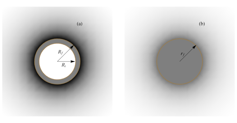
Figure 1: (a) Schematic picture of an eicheon in the metric (56) taking into account a vacuum polarization in the form of dark radiation, (b) an eicheon in the metric (48) looks like a solid sphere with a “dark radiation” of the finite energy density in the center.

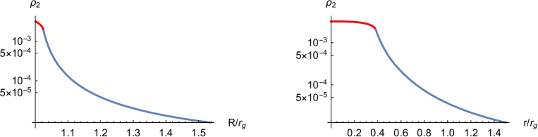
Figure 2: (a) $\rho_{2}$ – energy density of the vacuum polarization in a form of “dark radiation” in the coordinates $R>R_{i}$ calculated for the eicheon parameters $\rho_{1}=7M_{p}^{2}r_{g}^{-2}$, $R_{i}=1.001r_{g}$, $R_{f}=1.024r_{g}$, $\rho_{2}(R_{f})=0.002M_{p}^{2}r_{g}^{-2}$. Red part of the curve corresponds to $R_{i}<R<R_{f}$, i.e., lies inside an eicheon. (b) $\rho_{2}$ calculated in the coordinates $r$ of the metric (48). Red part of the curve corresponds to $0<r<r_{f}$.

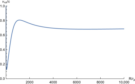
Figure 3: The general form of a model rotational curve for the eicheon parameters specified in the caption to Fig. 2.

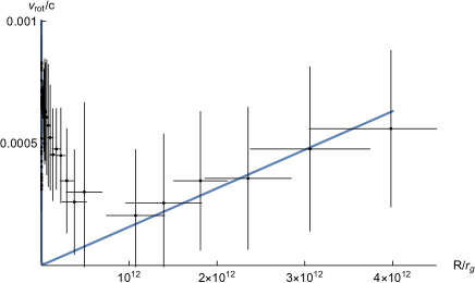
Figure 4: The rotational curve for the eicheon parameters $\rho_{1}=100M_{p}^{2}r_{g}^{-2}$, $R_{i}=1.0001r_{g}$ and $\rho_{2}(R_{f})=4\times 10^{-27}M_{p}^{2}r_{g}^{-2}$, where $r_{g}$ is defined by an eicheon mass. In the physical units $\rho_{1}=100\frac{3c^{6}}{16\pi G^{3}m_{\cdot}^{2}}\approx 2.1\times 10^{5}~{}g/cm^{3}$. The points and error bars correspond to the Milky Way rotational curve from [61].

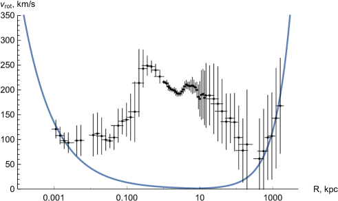
Figure 5: The rotational curve of eicheon with the mass of Sgr A^∗ with taking into account the vacuum polarization of $F$-type. The logarithmic scale is used and the points correspond to the Milky Way rotational curve from [61]. The eicheon parameters are given in the caption to Fig. 4.

Again, $\rho_{2}$ is measured in the terms of $r_{g}^{-2}M_{p}^{2}$, and $R$ is measured in the units of $r_{g}$. The solutions (57) and (55) are singular at $R=0$ and, thereby, nonphysical. The situation changes cardinally in the presence of a core consisting of incompressible matter. More exactly, in the presence of incompressible matter of low density $\rho_{1}$, the corresponding solution remains singular. However, if $\rho_{1}>\frac{1}{2}\left(\frac{8}{9}\right)$, a solid ball in the metric (48) looks like a shell over $r_{g}$ in the metric (56) [9] that is shown in Fig. 1 (a). Here, we again imply the gravitational radius $r_{g}$ as a measure of the distances, but calculate it taking into account only an incompressible matter. Such a matter occupies a region between $R_{i}$ and $R_{f}$, where

$$R_{f}=\sqrt[3]{R_{i}^{3}+\frac{1}{2\rho_{1}}}$$ (60)

in the units of $r_{g}$. Here the energy density $\rho_{1}$ is constant and measured in the terms of $r_{g}^{-2}M_{p}^{2}$, where the gravitational radius is defined as $r_{g}=\frac{3m_{1}}{2\pi M_{p}^{2}}$ and $m_{1}=\frac{4}{3}\pi\rho_{1}(R_{f}^{3}-R_{i}^{3})$. Compact object of such a type arising in FVT is known as ”eicheon” [9] and replaces a black hole of GR. The appearance of eicheon in the center makes the solution (58) to be nonsingular because it allows for setting the finite boundary conditions for radiation.

To explain this, let us consider two fluids in the metric (56) obeying the TOV equations:

$$p_{1}^{\prime}=-\frac{3(p_{1}+\rho_{1})\left(m+4\pi R^{3}\left(p_{1}+\frac{\rho_{2}}{3}\right)\right)}{4\pi R\left(R-\frac{3m}{2\pi}\right)},$$ (61)

$$\rho_{2}^{\prime}=-\frac{3\rho_{2}\left(m+4\pi R^{3}\left(p_{1}+\frac{\rho_{2}}{3}\right)\right)}{\pi R\left(R-\frac{3m}{2\pi}\right)},$$ (62)

where the function $m(R)$ satisfies to

$$m^{\prime}(R)=4\pi R^{2}(\rho_{1}+\rho_{2}).$$ (63)

For $\rho_{1}>\frac{1}{2}\left(\frac{8}{9}\right)$, the above equations hold for the internal range $R_{i}<R<R_{f}$, where $R_{i}>r_{g}$ and the border, occupied by $\rho_{1}$, is defined through (60).

The pressure of incompressible fluid must turn to zero at the edge of the range filled by matter $R=R_{f}$, and it is a boundary condition for $p_{1}$. Then, one could set an amount of radiation at $R=R_{f}$ and solve the system of equations in a region of $\{R_{i},R_{f}\}$ assuming $m(R_{i})=0$. A solution allows determining $m(R_{f})$, and, using this value as an initial condition, one should solve the equation for the radiation fluid (58) in an outer region of $\{R_{f},\infty\}$. The metric obtained by solving the equations is [58]

$$\frac{1}{B}\frac{dB}{dR}=-\frac{2}{p_{1}+\rho_{1}}\frac{dp_{1}}{dR}=-\frac{2}{p_{2}+\rho_{2}}\frac{dp_{2}}{dR},$$ (64)

$$\frac{d}{dR}\left(\frac{R}{A}\right)=1-{6}\,R^{2}(\rho_{1}+\rho_{2}).$$ (65)

Comparing the metric (46) and (56) leads to relation for the radial coordinates $R$ and $r$ [9]

$$\frac{dR}{dr}=\left(\frac{r}{R}\right)^{2}\frac{B^{3/2}}{A^{1/2}},$$ (66)

where the dependencies $B(R(r))$ and $A(R(r))$ are implied. Eq. (66) has to be integrated with the initial condition $R(0)=R_{i}$, which means that $R_{i}$ in the metric (56) corresponds to $r=0$ in the metric (46). Knowing $R(r)$ allows plotting $\rho_{2}(R)$ shown in Fig. 2 (a) as the $r$– dependent function $\rho_{2}(R(r))$ (Fig. 2 (b)).

Let us consider the motion of a test particle on a circular orbit in the metric (56). The angular velocity on a circular orbit is calculated as [58]:

$$\frac{d\phi}{dt}=\sqrt{\frac{1}{2R}\frac{dB}{dR}}.$$ (67)

A spatial interval followed by a particle along the circular orbit is given by $dl=Rd\phi=R\frac{d\phi}{dt}dt$. To obtain the rotation velocity observed by an observer situated at rest near the moving particle, one has to divide the spatial interval over the proper time $\sqrt{g_{00}}dt=\sqrt{B}dt$ of such an observer [62]:

$$v_{rot}=\frac{dl}{\sqrt{B}dt}=\sqrt{\frac{R}{2B}\frac{dB}{dR}}=\sqrt{-\frac{R}{p_{2}+\rho_{2}}\frac{dp_{2}}{dR}}=\frac{1}{2}\sqrt{-\frac{R}{\rho_{2}}\frac{d\rho_{2}}{dR}}.$$ (68)

A qualitative example of the general form of the numerical solution for the rotation velocity is shown in Fig. 3. Although the shape of the curve resembles observational data, asymptotic of the rotation curve corresponds to $v_{rot}\sim 1/\sqrt{2}\approx 0.71$. This very large velocity (in units of speed of light) corresponds to asymptotic value $\rho_{2}\sim R^{-2}$ in (57), whereas, in the reality, the rotation velocities of galaxies are $v_{rot}\sim 100-300~{}$km/s$~{}\sim 0.001$. To obtain smaller velocities, one has to diminish density of radiation in the center of eicheon, i.e. at $r=0$ in the metric (48) or $R=R_{i}$ in the metric (56). For central radiation density of $\rho_{2}=4.6\times 10^{-27}~{}M_{p}^{2}r_{g}^{-2}=9.6\times 10^{-24}~{}$g/$\mbox{cm}^{3}$, one has the rotation curve shown in Fig. 4. That is a pure “dark radiation” contribution without the galaxy bulge or disk. It increases linearly with the distance and corresponds to the rising part of the general curve shown in Fig. 3. In the logarithmic scale, one could see (Fig. 5) together the contribution of the eicheon of the mass of $4.2\times 10^{6}~{}M_{\bigodot}$ in the center of the Milky Way (the left side of the curve) and the impact of the dark radiation (the right side of the curve), whereas the effects of the galactic bulge and disk responsible for the intermediate region are not taken into account. However, it is expected that bulge and disk attraction will influence the $F$-type vacuum polarization in such a way that the curve in Fig. 4 will be not pure linear but slightly bent. We do not gain insight into such details because our goal is to show that the $F$-type vacuum polarization could arise only around a “sewed” black hole, i.e., around eicheon.

We emphasize that the presented consideration is heuristic because, although the linear system for the perturbation and the eikonal approximation for vacuum polarization seems reasonable, we use its results in the nonlinear TOV model. Another thing is that we set the density of radiation (the $F$-type vacuum polarization) in the center of eicheon, i.e., at $r=0$, of $R=R_{i}$ empirically but not calculate it from the first principles, i.e., we use only the equation of state obtained from the calculations in the eikonal approximation.

VI Vacuum polarization of $\Phi$-type

In Sections III, IV the linear system of equation (20),(21),(22),(23),(41) was deduced, which describes the evolution of perturbation by taking into account vacuum polarization (see Eq. (41)). Galaxy formation is a complex nonlinear process that develops over cosmological time scales. Generally, the linear system is insufficient to describe the galaxy evolution. However, one could create a heuristic picture setting an approximate profile of matter near the galaxy center and obtain a gravitational potential produced by vacuum polarization obeying the linear equations. Below we will discuss that the observed galaxy halo could originate from a very fast (compared to the cosmological times) growth of the galactic nucleus mass. We will neglect a cosmological evolution assuming $\alpha(\eta)=0$. That reduces the above system of the equations to

$$-12\Phi_{\bm{q}}-3F_{\bm{q}}^{\prime\prime}+q^{2}F_{\bm{q}}=0,$$ (69)

$$-9\Phi_{\bm{q}}^{\prime\prime}-9q^{2}\Phi_{\bm{q}}+q^{4}F_{\bm{q}}+\frac{9}{M_{p}^{2}}\left(\sum_{i}\delta\wp_{\bm{k}i}-3\delta\Pi_{\bm{q}i}\right)=0.$$ (70)

$$\delta\wp_{\bm{q}v}-3\delta\Pi_{\bm{q}v}=\frac{N_{sc}}{8\pi^{2}}k_{max}^{2}(\Phi^{\prime\prime}_{\bm{q}}+q^{2}\Phi_{\bm{q}}),$$ (71)

where the last equation holds for the vacuum polarization of $\Phi$–type and is denoted by $i=v$. Substituting $\Phi_{\bm{q}}$ from Eq. (69), and $\delta\wp_{\bm{q}v}-3\delta\Pi_{\bm{q}v}$ from Eq. (71) into Eq. (70) gives the equation

$$3\left({k_{max}}^{2}-8\pi^{2}{M_{p}}^{2}\right)\left(3F^{\prime\prime\prime\prime}_{\bm{q}}+2q^{2}F_{\bm{q}}^{\prime\prime}\right)-q^{4}F_{\bm{q}}\left(3N_{sc}{k_{max}}^{2}+8\pi^{2}{M_{p}}^{2}\right)=288\pi^{2}{\delta\wp_{\bm{q}\,eff}}(\eta),$$ (72)

where an effective “density” of all the substances except vacuum is denoted as

$$\delta\wp_{\bm{q}\,eff}(\eta)=\sum_{i\neq v}\delta\wp_{\bm{k}i}-3\delta\Pi_{\bm{q}i}.$$ (73)

Eq. (72) allows developing a simple model: setting profile and time dependencies of the quantity $\wp_{\bm{q}\,eff}(\eta)$ empirically allows finding the metric perturbation $F_{\bm{q}}$ and calculate $\Phi_{\bm{q}}$ using (69), i.e., to determine the gravitational field corresponding to $\wp_{\bm{q}\,eff}(\eta)$.

Let us, for simplicity, take $\wp_{\bm{q}\,eff}(\eta)$ in the form of

$$\wp_{\bm{q}\,eff}(\eta)=m\,Z(q)e^{\eta/T},$$ (74)

where $m$ is a “mass” of the object at $\eta=0$, $Z(q)$ is a form-factor and $T$ is some typical time of the “mass” growth. The model implies some rapid processes like accretion occurring around the massive object, i.e., around the galaxy nucleus. Substitution of the expression (74) into Eq. (72) allows finding $F_{\bm{q}}(\eta)=\tilde{F}_{\bm{q}}e^{\eta/T}$, where

$$\tilde{F}_{\bm{q}}=-\frac{288\pi^{2}T^{4}mZ(q)}{3N_{sc}{k_{max}}^{2}\left(q^{4}T^{4}-2q^{2}T^{2}-3\right)+8\pi^{2}{M_{p}}^{2}\left(q^{2}T^{2}+3\right)^{2}},$$ (75)

and Eq. (69) give $\Phi_{\bm{q}}(\eta)=\tilde{\Phi}_{\bm{q}}e^{\eta/T}$:

$$\tilde{\Phi}_{\bm{q}}=-\frac{24\pi^{2}T^{2}\left(q^{2}T^{2}-3\right)mZ(q)}{3N_{sc}{k_{max}}^{2}\left(q^{4}T^{4}-2q^{2}T^{2}-3\right)+8\pi^{2}{M_{p}}^{2}\left(q^{2}T^{2}+3\right)^{2}}.$$ (76)

At $T\rightarrow\infty$, the corresponding static limit is

$$\tilde{\Phi}_{\bm{q}}=-\frac{24\pi^{2}mZ(q)}{(3N_{sc}{k_{max}}^{2}+8\pi^{2}{M_{p}}^{2})q^{2}},$$ (77)

which implies that the vacuum polarization leads to renormalization (increasing) of the Planck mass, i.e., decreasing the gravitational constant. In particular, using the value (11) obtained from the cosmological observations [10] gives

$$M_{p\,ren}^{2}=\left(1+\frac{54N_{sc}}{\pi^{2}(2+N_{sc})}\right)M_{p}^{2},~{}~{}~{}~{}~{}~{}~{}~{}~{}G_{ren}=G/\left(1+\frac{54N_{sc}}{\pi^{2}(2+N_{sc})}\right).$$ (78)

It seems that the vacuum polarization, in some sense, acts like antigravitation, and the gravitational constant $G_{ren}$ appearing in Newton’s law has to differ from the gravitational constant $G$ in the Friedmann equations for a uniform universe. Although the gravitational constant’s renormalization does not influence the cosmological balance of the different kinds of matter expressed in the units of the critical density $M_{p}^{2}H^{2}$, it should be taken into account for comparison with the directly measured (for instance, utilizing luminosity) density. Numerically $N_{sc}=2$ gives $G_{ren}\approx 0.27\,G$.

VI.1 Invariant potentials and rotational curves

Astrophysicists express the results of observations in terms of gauge-invariant quantities, which are not dependent on system of coordinates. The potentials $\Phi(\eta,\bm{x})$ and $F(\eta,\bm{x})$ are not invariant relatively the infinitesimal transformations of coordinates and time of the following type

$$t=\eta+\xi_{1}(\eta,\bm{x}),~{}~{}~{}~{}~{}~{}~{}~{}~{}~{}~{}~{}~{}\bm{r}=\bm{x}+\bm{\nabla}\xi_{2}(\eta,\bm{x}),$$ (79)

where $\xi_{1}(\eta,\bm{x})$ and $\xi_{2}(\eta,\bm{x})$ are some small functions. Usually the potentials $\Phi_{inv}(\eta,\bm{x})$ and $\Psi_{inv}(\eta,\bm{x})$ are introduced [63, 64, 65] which are invariant relatively transformations (79). The potentials correspond to the metric

$$ds^{2}=a^{2}(\eta)\left((1+2\Phi_{inv}(\eta,\bm{x}))d\eta^{2}-\left(1-2\Psi_{inv}(\eta,\bm{x})\right)\delta_{ij}dx^{i}dx^{j}\right)$$ (80)

and are expressed through $\Phi$ and $F$ as

$$\Phi_{\bm{q}\,inv}(\eta)=\Phi_{\bm{q}}(\eta)+\frac{a^{\prime}(\eta)F_{\bm{q}}^{\prime}(\eta)+a(\eta)F_{\bm{q}}^{\prime\prime}(\eta)}{2a(\eta)}=\Phi_{\bm{q}}+\frac{F_{\bm{q}}}{2T^{2}},$$ (81)

$$\Psi_{\bm{q}\,inv}(\eta)=-\frac{a^{\prime}(\eta)F_{\bm{q}}^{\prime}(\eta)}{2a(\eta)}-\Phi_{\bm{q}}(\eta)+\frac{1}{6}q^{2}F_{\bm{q}}(\eta)=-\Phi_{\bm{q}}(\eta)+\frac{1}{6}q^{2}F_{\bm{q}},$$ (82)

where the final equalities at the right-hand side of (81), (82) hold for our case of $a=const$, and $\Phi,F\sim\exp\left(\eta/T\right)$. Using (75), (76) gives

$$\tilde{\Phi}_{\bm{q}\,inv}=-\frac{24\pi^{2}T^{2}\left(q^{2}T^{2}+3\right)m\,Z(q)}{3N_{sc}\,{k_{max}}^{2}\left(q^{4}T^{4}-2q^{2}T^{2}-3\right)+8\pi^{2}{M_{p}}^{2}\left(q^{2}T^{2}+3\right)^{2}},$$ (83)

and $\tilde{\Psi}_{\bm{q}\,inv}=\tilde{\Phi}_{\bm{q}\,inv}$. Thus, we obtained the Fourier transformation of the time-dependent gravitational potential $\Phi_{\bm{q}\,inv}=\tilde{\Phi}_{\bm{q}\,inv}e^{\eta/T}$ allowing us to define

$$\Phi_{inv}(\bm{x},\eta)=\frac{e^{\eta/T}}{(2\pi)^{3}}\int\tilde{\Phi}_{\bm{q}\,inv}\,e^{i\bm{q}\bm{x}}d^{3}\bm{q}.$$ (84)

To obtain a concrete empirical formula, one has to set the form factor $Z(q)$, for instance, using the Gaussian profile $\delta\tilde{\wp}_{eff}(\bm{x})=\pi^{-3/2}m\,D^{-3}\,e^{-x^{2}/D^{2}}$. The spatial dependence of the potential (84) at the present time, i.e., $\eta=0$ allows us to find the rotational velocity dependence on the spatial coordinate

$$v_{rot}(r)=\sqrt{-r\frac{d\Phi_{inv}(r)}{dr}}.$$ (85)

Here, the potential (84) is time-dependent, and actually, there are no pure rotational curves because the radial velocities are present. Here, for an estimation, we discuss only tangential velocity. The parameters $m$, $D$ and $Z(q)$ are adopted to produce a typical rotational curve without an DM (blue curve in Fig. 6), then vacuum polarization produces a halo corresponding to black curve in Fig. 6.

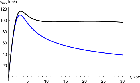
Figure 6: The lower blue curve corresponds to the contribution of a galactic nucleus of baryonic matter, including specifically nucleus, bulge, and disk. The upper black curve takes the vacuum $\Phi$-polarization into account. The form factor of a galaxy nuclei is taken as $Z(q)-\exp\left(-\lambda q^{2}\right)$, $\lambda=1$, the accretion rate is of $T=10$, i.e., $10$ kPc, which corresponds to 32000 years. Number of the minimally coupled scalar fields is of $N_{sc}=2$, and $k_{max}^{2}=8M_{p}^{2}\pi^{2}\frac{98}{100}$ is assumed.

.

The rotational curve has some similarities with the conventional picture at $N_{sc}=2$, but in the conventional picture, the contribution of the galactic nucleus, bulge, and disk are taken into account. We include all these components into the Gaussian form factor of galactic baryonic skeleton and call it ”nucleus” in our oversimplified picture. Then we permit it to increase (or decrease) with time and obtain vacuum polarization caused by this process.

VII Conclusion

We have considered two types of vacuum polarization corresponding to the $F$- and $\Phi$-types of metric perturbations in the CUM frame.

The $F$-type of spatially-nonuniform vacuum polarization has the radiation-type equation of state. In the first order on perturbations, it is impossible to determine a form of the static gravitational potential around an astrophysical object. In the frameworks of a nonlinear heuristic model using the TOV equations for matter and radiation, it was found that the solution, which is nonsingular at $r=0$, only arises if an eicheon is present in the galaxy’s center. Eicheon is an analog of the black hole in GR and looks like an empty “nut” in the Schwarzschild type metric. From this point of view, we assume that DM, as a vacuum polarization, arises only in the galaxies having an eicheon (i.e., a “black hole-like” object) in the center. Namely, the eicheon conjecture allows us to convert a singular solution for pure radiation into a nonsingular physical one. Galaxies without an eicheon in the center (e.g., diffuse galaxies) is not to have a DM halo .

Under the oversimplified assumption of an isolated galaxy, the dark halo, in terms of a test particle’s rotation velocity, always increases with the distance from the galaxy’s center. Decreasing the halo could occur only due to a violation of the galaxy’s isolation, i.e., at the distance of $\sim~{}$2 Mpc. It should be noted that the Andromeda galaxy is only 0.7 Mpc away. Generally, the galaxies tend to form clusters. These evident facts urge the development of a model of interacting galaxies with vacuum polarization.

For the $\Phi$-type of vacuum polarization, the renormalization of the gravitational constant (or Planck mass) has been found. That means that the gravitational constant found in the Earth, the Solar system, and galaxy observations is not equal (approximately four times less) to the gravitational constant used in cosmology to describe a spatially uniform universe. This fact does not influence the balance of the different kinds of matter in cosmology if one measures them in $M_{p}^{2}H^{2}$. Nevertheless, it increases the directly counted matter contribution fourfold, i.e., the luminous baryonic matter has to contribute $3.7$-times stronger into the cosmological Friedmann equations.

The second effect of the $\Phi$-type polarization is the creation of the dark halo in the nonstationary process. It is found that the time-dependent evolving mass of the galaxy nuclei produces the gravitational potential of the dark halo type. This point urges a more careful observational investigation of the possible nonstationary origin of the dark halo. However, the required time for the galaxy nuclei mass growth seems very short $\sim 32000$ years. In such a situation, clarifying the physical status of the possible accretion of vacuum energy and vacuum condensates discussed in [68, 69, 70] is very desirable. In particular, it was shown in [68, 69] that accretion of substance with the equation of state of $p=-\rho$ (e.g., Higgs or QCD condensates) decreases a black hole mass, while accretion of the ordinary substance with radiation equation of state increases a black hole mass.

Investigations of these processes in the CUM metric with the applications to an eicheon are waiting. However, one may suggest some scenarios of a galaxy center evolution. Accretion by an eicheon could be more complicated than a traditional black hole. At some stage, eicheon could accrete more “dark radiation”, increasing its mass, but at some stage, it could accrete more condensates, decreasing its mass. One could associate this with the fast processes with a typical time of $\sim 32000$ years. Both growth of the galaxy’s center mass and its lowering produce a halo. Thus, a galaxy center reminds “Alice from Wonderland” [71], which takes a bit of a mushroom from one side and rises then takes a bit from another side and shrinks. These processes can interlace in a galaxy center.

To summarize, it is possible to obtain an equation of the state of vacuum polarization, which is some kind of “æther”. It is challenging to find the “amount” of æther because it depends on the object’s entire history due to the nonlocality of the vacuum state on the curved background. Here we have adjusted this “amount” to astrophysical observations. Thus, the obtained final results have, in some sense, a heuristic nature.

Acknowledgements

We are grateful to Yoshiaki Sofue for a permission to use the results of his observation of Milky Way rotational curve in FIG. 4 and FIG 5.

References

- Weinberg [1989] S. Weinberg, Rev. Mod. Phys. 61, 1 (1989).
- Peebles and Ratra [2003] P. J. E. Peebles and B. Ratra, Rev. Mod. Phys. 75, 559 (2003).
- Mostepanenko and Klimchitskaya [2019] V. M. Mostepanenko and G. L. Klimchitskaya, Symmetry 11, 10.3390/sym11030314 (2019).
- Unruh and Wald [2017] W. Unruh and R. Wald, Rep. Progr. Phys. 80, 092002 (2017).
- Chakraborty and Lochan [2017] S. Chakraborty and K. Lochan, Universe 3, 10.3390/universe3030055 (2017).
- Mizner et al. [1973] C. W. Mizner, K. Thorne, and J. A. Wheeler, Gravitation, Vol. 1 (Freeman, San Francisco, USA, 1973).
- Landau and Lifshitz [1975] L. D. Landau and E. Lifshitz, The Classical Theory of Fields, Vol. 2 (Butterworth-Heinemann, Oxford, 1975).
- Cherkas and Kalashnikov [2019] S. L. Cherkas and V. L. Kalashnikov, Proc. Natl. Acad. Sci. Belarus, Ser. Phys.-Math. 55, 83 (2019), arXiv:1609.00811 [gr-qc] .
- Cherkas and Kalashnikov [2020a] S. L. Cherkas and V. L. Kalashnikov, Phys. Scr. 95, 085009 (2020a).
- Haridasu et al. [2020] B. S. Haridasu, S. L. Cherkas, and V. L. Kalashnikov, Fortschr. Phys. 68, 2000047 (2020), arXiv:1912.09224 .
- Cherkas and Kalashnikov [2008] S. L. Cherkas and V. L. Kalashnikov, in Proc. Int. conf. “Problems of Practical Cosmology”, Saint Petersburg, June 23 - 27, 2008 (2008) pp. 135–140, arXiv:0611795 [astro-ph] .
- Iorio [2006] L. Iorio, JCAP 2006 (05), 002.
- Freese [2009] K. Freese, EAS Publications Series 36, 113 (2009).
- Oks [2021] E. Oks, New Astron. Rev. 93, 101632 (2021).
- Weinberg et al. [2015] D. H. Weinberg, J. S. Bullock, F. Governato, R. Kuzio de Naray, and A. H. Peter, Proc. Natl. Acad. Sci. 112, 12249 (2015).
- de Martino et al. [2020] I. de Martino, S. S. Chakrabarty, V. Cesare, A. Gallo, L. Ostorero, and A. Diaferio, Universe 6, 107 (2020).
- Bertone et al. [2005] G. Bertone, D. Hooper, and J. Silk, Phys. Rep. 405, 279 (2005).
- Buchmueller et al. [2017] O. Buchmueller, C. Doglioni, and L.-T. Wang, Nature Phys. 13, 217 (2017).
- Aprile et al. [2022] E. Aprile et al., Search for new physics in electronic recoil data from xenonnt (2022), arXiv:2207.11330 [hep-ex] .
- Albareti et al. [2014] F. Albareti, J. Cembranos, and A. Maroto, Phys. Rev. D 90, 123509 (2014).
- Hajdukovic [2012] D. S. Hajdukovic, Astrophysics and Space Science 337, 9 (2012).
- Penner [2016] A. R. Penner, Astrophysics & Space Science 361, 1 (2016).
- Hajdukovic [2019] D. Hajdukovic, MNRAS 491, 4816 (2019).
- Fiscaletti [2020] D. Fiscaletti, J. Theor. Appl. Phys. 14, 203 (2020).
- Penner [2022] A. R. Penner, Class. Quant. Grav. 39, 075001 (2022).
- Blanchet and Le Tiec [2008] L. Blanchet and A. Le Tiec, Phys. Rev. D 78, 024031 (2008).
- Chardin et al. [2021] G. Chardin, Y. Dubois, G. Manfredi, B. Miller, and C. Stahl, Astron. Astrophys. 652, A91 (2021).
- Huang [2016] K. Huang, A superfluid Universe (World Scientific, 2016).
- Sbitnev [2015] V. I. Sbitnev, Mod. Phys. Lett. A 30, 1550184 (2015).
- Zloshchastiev [2020] K. G. Zloshchastiev, Universe 6, 180 (2020).
- Hamber and Liu [1995] H. Hamber and S. Liu, Phys. Lett. B 357, 51 (1995).
- Bonanno and Reuter [2000] A. Bonanno and M. Reuter, Phys. Rev. D 62, 043008 (2000).
- Ward [2002] B. Ward, Mod. Phys. Lett. A 17, 2371 (2002).
- Kirilin and Khriplovich [2002] G. G. Kirilin and I. B. Khriplovich, JETP 95, 981 (2002).
- Satz et al. [2005] A. Satz, F. D. Mazzitelli, and E. Alvarez, Phys. Rev. D 71, 10.1103/physrevd.71.064001 (2005).
- Morley et al. [2021] T. Morley, W. E., and T. P., Phys. Rev. D 103, 10.1103/physrevd.103.045007 (2021).
- Birrell and Davis [1982] N. D. Birrell and P. C. W. Davis, Quantum Fields in Curved Space (Cambridge University Press, Cambridge, England, 1982).
- Arnowitt et al. [2008] R. Arnowitt, S. Deser, and C. W. Misner, Gen. Rel. Grav. 40, 1997 (2008).
- Cherkas and Kalashnikov [2015] S. L. Cherkas and V. L. Kalashnikov, Nonlin. Phenom. Complex Syst. 18, 1 (2015), arXiv:1302.2229 [gr-qc] .
- Cherkas and Kalashnikov [2020b] S. L. Cherkas and V. L. Kalashnikov, J. Belarusian State Univ. Physics 3, 97 (2020b).
- Cherkas and Kalashnikov [2007] S. L. Cherkas and V. L. Kalashnikov, JCAP 01, 028, arXiv:0610148 [gr-qc] .
- Cherkas and Kalashnikov [2021a] S. L. Cherkas and V. L. Kalashnikov, Vestnik Brest Univ., Ser. Fiz.-Mat. 1, 41 (2021a), arXiv:1810.06211 [gr-qc] .
- Visser [2018] M. Visser, Particles 1, 138 (2018).
- Visser [2019] M. Visser, Phys. Lett. B 791, 43 (2019).
- Workman et al. [2022] R. L. Workman et al. (Particle Data Group), PTEP 2022, 083C01 (2022).
- Cherkas and Kalashnikov [2020c] S. Cherkas and V. Kalashnikov, Nonlin. Phenom. Complex Syst. 23, 332 (2020c), arXiv:1810.06211 [gr-qc] .
- Mattingly [2005] D. Mattingly, Liv. Rev. Rel. 8, 1 (2005).
- Amelino-Camelia [2013] G. Amelino-Camelia, Liv. Rev. Rel. 16, 1 (2013).
- Bluhm and Yang [2021] R. Bluhm and Y. Yang, Symmetry 13, 660 (2021).
- Anber et al. [2010] M. M. Anber, U. Aydemir, and J. F. Donoghue, Phys. Rev. D 81, 084059 (2010).
- Mavromatos [2004] N. E. Mavromatos, in Beyond the Desert 2003 (Springer, 2004) pp. 43–72.
- Nilsson [2020] N. A. Nilsson, Aspects of Lorentz and CPT Violation in Cosmology, Ph.D. thesis, National Centre for Nuclear Research, Otwock-Świerk (2020).
- Cherkas and Kalashnikov [2018] S. L. Cherkas and V. L. Kalashnikov, in Fractional Dynamics, Anomalous Transport and Plasma Science, edited by C. H. Skiadas (Springer, Cham, 2018) Chap. 9.
- Dirac [1951] P. A. M. Dirac, Nature 168, 906 (1951).
- Cherkas and Kalashnikov [2021b] S. L. Cherkas and V. L. Kalashnikov, Phys. Scr. 96, 115001 (2021b), arXiv:2012.02288 [gr-qc] .
- Czyz and Maximon [1969] W. Czyz and L. Maximon, Ann. Phys. (NY) 52, 59 (1969).
- Kabat and Ortiz [1992] D. Kabat and M. Ortiz, Nucl. Phys. B 388, 570 (1992).
- Weinberg [1972] S. Weinberg, Gravitation and Cosmology: Principles and Applications of the General Theory of Relativity (John Wiley & Sons, New York, 1972).
- Tolman [1939] R. C. Tolman, Phys. Rev. 55, 364 (1939).
- Oppenheimer and Volkoff [1939] J. R. Oppenheimer and G. M. Volkoff, Phys. Rev. 55, 374 (1939).
- Sofue [2013] Y. Sofue, Publ. Astron. Soc. Jpn. 65, 10.1093/pasj/65.6.118 (2013), 118.
- Rahaman et al. [2010] F. Rahaman, K. Nandi, A. Bhadra, M. Kalam, and K. Chakraborty, Phys. Lett. B 694, 10 (2010).
- Riotto [2002] A. Riotto, in Proc. Summer School on Astroparticles Physics and Cosmology, Trieste, 17 June - 5 July, 2002 (2002) pp. 317–417, arXiv:0210162 [hep-ph] .
- Hu [2004] W. Hu, in Proc. Summer School on Astroparticles Physics and Cosmology, Trieste, 17 June - 5 July, 2002 (2004) pp. 147–185, arXiv:0402060 [astro-ph] .
- Mukhanov [2005] V. Mukhanov, Physical Foundations of Cosmology (Cambridge University Press, Cambridge, England, 2005).
- Van Dokkum et al. [2018] P. Van Dokkum, S. Danieli, Y. Cohen, A. Merritt, A. J. Romanowsky, R. Abraham, J. Brodie, C. Conroy, D. Lokhorst, L. Mowla, E. O’Sullivan, and J. Zhang, Nature 555, 629 (2018).
- Van Dokkum et al. [2016] P. Van Dokkum, R. Abraham, J. Brodie, C. Conroy, S. Danieli, A. Merritt, L. Mowla, A. Romanowsky, and J. Zhang, Astr. J. Lett. 828, L6 (2016).
- Babichev et al. [2004] E. Babichev, V. Dokuchaev, and Y. Eroshenko, Phys. Rev. Lett. 93, 021102 (2004).
- Babichev [2005] E. O. Babichev, JETP 100, 528 (2005).
- Cheng-Yi [2009] S. Cheng-Yi, Comm. Theor. Phys. 52, 441 (2009).
- Carroll [2015] L. Carroll, Alice’s Adventures in Wonderland (Princeton University Press, Princeton, USA, 2015).