Programming with Context-Sensitive Holes using Dependency-Aware Tuning

Abstract.

Developing efficient and maintainable software systems is both hard and time consuming. In particular, non-functional performance requirements involve many design and implementation decisions that can be difficult to take early during system development. Choices—such as selection of data structures or where and how to parallelize code—typically require extensive manual tuning that is both time consuming and error-prone. Although various auto-tuning approaches exist, they are either specialized for certain domains or require extensive code rewriting to work for different contexts in the code. In this paper, we introduce a new methodology for writing programs with holes, that is, decision variables explicitly stated in the program code that enable developers to postpone decisions during development. We introduce and evaluate two novel ideas: (i) context-sensitive holes that are expanded by the compiler into sets of decision variables for automatic tuning, and (ii) dependency-aware tuning, where static analysis reduces the search space by finding the set of decision variables that can be tuned independently of each other. We evaluate the two new concepts in a system called Miking, where we show how the general methodology can be used for automatic algorithm selection, data structure decisions, and parallelization choices.

1. Introduction

Software developers constantly face implementation choices that affect performance, such as choices of data structures, algorithms, and parameter values. Unfortunately, traditional programming languages lack support for expressing such alternatives directly in the code, forcing the programmer to commit to certain design choices up front. To improve the performance of a program, a developer can profile the code and manually tune the program by explicitly executing the program repeatedly, testing and changing different algorithm choices and parameter settings. However, such manual tuning is both tedious and error prone because the number of program alternatives grows exponentially with the number of choices. Besides choices of program parameters, hardware properties, such cache layout and core configurations make manual optimization even more challenging.

An attractive alternative to manual tuning of programs is to perform the tuning automatically. Conceptually, a tuning problem is an optimization problem where the search space consists of potential program alternatives and the goal is to minimize an objective, such as execution time, memory usage, or code size. The search space is explored using some search technique, which can be performed either offline (at compile-time) or online (at runtime). In this work, we focus on offline tuning.

Several offline auto-tuning tools have been developed to target problems in specific domains. For instance, ATLAS (Whaley, 2011) for linear algebra, FFTW (Frigo, 1999) and SPIRAL (Franchetti et al., 2018) for linear digital processing, PetaBricks (Ansel et al., 2009) for algorithmic choice, as well as tools for choosing sorting algorithm automatically (Li et al., 2004). Although these domain-specific tuning approaches have shown to work well in their specific area, they are inherently targeting a specific domain and cannot be used in general for other kinds of applications.

In contrast to domain-specific tuning, generic auto-tuners offer solutions that work across domains and may be applicable to arbitrary software systems. For instance, approaches such as ATF (Rasch and Gorlatch, 2019), OpenTuner (Ansel et al., 2014), CLTune (Nugteren and Codreanu, 2017), HyperMapper (Nardi et al., 2019), and PbO (Hoos, 2012) make it possible for developers to specify unknown variables and possible values. The goal of the tuner is then to assign values to these variables optimally, to minimize for instance execution time. In particular, existing generic auto-tuners assign values to variables globally, i.e., each unknown variable is assigned the same value throughout the program.

In this work, we focus on two problems with state-of-the-art methods. Firstly, only using global decision variables does not scale in larger software projects and it violates fundamental software engineering principles. Specifically, a global decision variable does not take into consideration the context from where a function may be called. Global decision variables can of course be manually added in all calling contexts, but such manual refactoring of code makes code updates brittle and harder to maintain. Secondly, auto tuning is typically computationally expensive, since the search space consists of all combinations of decision variable values. This is because decision variables are dependent on each other in general. However, if a subset of the decision variables is independent, then the auto tuner wastes precious time exploring unnecessary configurations.

In this paper, we introduce a methodology where a software developer postpones design decisions during code development by explicitly stating holes in the program. A hole is a decision variable for the auto tuner, with a given default value and domain, such as integer range or Boolean type. In contrast to existing work, we introduce context-sensitive holes. This means that a hole that is specified in a program (called a base hole) can be expanded into a set of decision variables (called context holes) that take the calling context into consideration. The compiler statically analyses the call graph of the program and transforms the program so that the calling context is maintained during runtime. Only paths through the call graph up to a certain length are considered, to avoid a combinatorial explosion in the number of variables.

In our approach, context-sensitive holes can be automatically tuned using input data, without manual involvement. We develop and apply a novel static dependency analysis to build a bipartite dependency graph, which encodes the dependencies among the context-sensitive holes. In contrast to existing approaches, the dependency analysis is automatic, though optional annotations may be added to increase the accuracy. The dependency graph is used to reduce the search space in a method we call dependency-aware tuning. Using this method, the auto tuner concentrates its computation time on exploring only the necessary configurations of hole values.

Specifically, we make the following contributions:

• We propose a general methodology for programming with context-sensitive holes that enables the software developer to postpone decisions to a later stage of automatic tuning. In particular, we discuss how the methodology can be used for algorithm and parallelization decisions (Section 2).

• To enable the proposed methodology, we propose a number of algorithms for performing program transformations for efficiently maintaining calling context during runtime (Section 3).

• We design and develop a novel static dependency analysis, and use the result during tuning to reduce the search space of the problem (Sections 4–5).

• We design and develop a complete solution for the proposed idea within the Miking framework (Broman, 2019), a software framework for developing general purpose and domain-specific languages and compilers (Section 6).

To evaluate the approach, we perform experiments on several non-trivial case studies that are not originally designed for the approach (Section 7).

2. Programming with Context-Sensitive Holes

In this section, we first introduce the main idea behind the methodology of programming with holes. We then discuss various programming examples, using global and context-sensitive holes.

2.1. Main Idea

Traditionally, an idea is implemented into a program by making a number of implementation choices, and gradually reducing the design space. By contrast, when programming with holes, we delay the decision of implementation choices. Design choices—such as what parts of the program to parallelize or which algorithms to execute in different circumstances—are instead left unspecified by specifying holes, that is, decision variables stated directly in the program code. Instead of taking the design decision up-front, an auto-tuner framework makes use of input data and runtime profiling information, to make decisions of filling in the holes with the best available alternatives. Thus, the postponed decisions can be automated and based on more information, resulting in less ad hoc and more informed decisions.

2.2. Global Holes

The key concept in our methodology is the notation of holes. A hole is an unknown variable whose optimal value is to be decided by the auto-tuner, defined in a program using the keyword hole. The hole takes as arguments the type of the hole (either Boolean or IntRange) and its default value. Additionally, the IntRange type expects a minimum and maximum value.

Example 2.1.

To illustrate the idea of a hole, we first give a small example illustrating how to choose sorting algorithms based on input data length. Consider the following program, implemented in the Miking core language:

⬇

6let sort = lam seq.

7 let threshold = hole (IntRange --*\label{l:sort1}*--

8 {default = 10, min = 0, max = 10000}) in --*\label{l:sort2}*--

9 if leqi (length seq) threshold then insertionSort seq --*\label{l:sort-ite-1}*--

10 else mergeSort seq --*\label{l:sort-ite-2}*--

The example defines a function sort using the let construction. The function has one parameter seq, defined using an anonymous lambda function lam. Lines LABEL:l:sort1–LABEL:l:sort2 define a hole with possible values in the range $[0,10000]$ and default value $10$. The program then chooses to use insertionSort if the length of the sequence is less than the threshold, and mergeSort otherwise. That is, an auto-tuner can use offline profiling to find the optimal threshold value that gives the overall best result. Note also that the default value can be used if the program is compiled without the tuning stage. ∎

The example above illustrates the use of a global hole, i.e., a hole whose value is chosen globally in the program. Although global holes are useful, they do not take into consideration the calling context.

2.3. Context-Sensitive Holes

All holes that are explicitly stated in the program code using the hole syntax represent base holes. As illustrated in the previous example, a base hole that does not take into consideration the calling context is the same thing as a global hole. One of the novel ideas in this paper is the concept of context-sensitive holes. In contrast to a global hole, the value of a context-sensitive hole varies depending on which call path is taken to the place in the program where the hole is defined. They are useful in programs where we believe the optimal value of the hole varies depending on the context. Context-sensitive holes are implicitly defined from a base hole, taking into consideration the different possible call paths reaching the base hole. The idea is illustrated with the following example.

Example 2.2.

Consider the higher-order function map, which applies a function f to all elements in a sequence s. The function can be applied either sequentially or in parallel (given that f is side-effect free). The optimal choice between the sequential or parallel version likely depends partly on the length of the sequence, but also on the nature of the function f. In a large program, a common function such as map is probably called from many different places in the program, with varying functions f and sequences. Therefore, globally deciding whether to use the sequential or parallel version may result in suboptimal performance. ∎

To define a context-sensitive hole, we provide an additional (optional) field depth, which represents the length of the most recent function call history that should influence the choice of the value of the hole.

Example 2.3.

The following is an implementation of map that chooses between the parallel and sequential versions (pmap and smap, respectively).

⬇

5let map = lam f. lam s.

6 let par = hole (Boolean {default = false, depth = 1}) in --*\label{l:bool-hole2}*--

7 if par then pmap f s else smap f s --*\label{l:par-ite}*--

Line LABEL:l:bool-hole2 defines a Boolean hole par with default value false (no parallelization). The depth = 1 tells the tuner that the value of par should consider the call path one step backward. That is, two calls to map from different call locations can result in different values of par.∎

Example 2.4.

Given that we choose the parallel map pmap in Example 2.3, another choice is how many parts to split the sequence into, before mapping f to each part in parallel. We can implement this choice with an integer range hole that represents the chunkSize, i.e. the size of each individual part.

⬇

25let pmap = lam f. lam s.

26 let chunkSize = hole (IntRange

27 {default = 10000, depth = 2, min = 1, max = 1000000000}) in

28 let chunks = split s chunkSize in

29 let tasks = smap (lam chunk.

30 async (lam. smap f chunk)) chunks in

31 join (smap await tasks)

Function split splits the sequence s into chunks of size (at most) chunkSize, that async sends the tasks to a thread pool, and that await waits for the tasks to be finished.

Note the choice of depth = 2 in this example. We expect the function pmap to be called from map, which has depth = 1. Since we want to capture the context from map we need to increment the depth parameter by one.∎

The choice of the depth parameter for a hole should intuitively be based on the number of function calls backward that might influence the choice of the value of the hole. A larger depth might give a better end result, but it also gives a larger search space for the automatic tuner, which influences the tuning time.

Note that in order to use global holes to encode the same semantics as the context-sensitive holes, we need to modify the function signatures. For example, in Example 2.3, which has a hole of depth $1$, we can let map take par as a parameter, and pass a global hole as argument each time we call map. For holes of depth $d>1$, this strategy becomes even more cumbersome, as each function along a call path need to pass on global holes as arguments. By instead letting the compiler handle the analysis of contexts, we do not need to modify function signatures, and we can easily experiment with the depth parameter. Additionally, holes can be “hidden” inside libraries, so that a user does not need to be aware of where the holes are defined, but still benefit from context-sensitive tuning. Another advantage of context-sensitive holes compared to global holes is that the compiler may use the knowledge that two context holes originate from the same base hole to speed up the tuning stage.

3. Program Transformations

This section covers the program transformations necessary for maintaining the context of each hole during runtime of the program. The aim of the program transformations is that the resulting program maintain contexts at a minimum runtime overhead. Sections 3.1 and 3.2 provide definitions and a conceptual illustration of contexts, while Section 3.3 covers the implementation in more detail.

3.1. Definitions

Central in our discussion of contexts are call graphs. Given a program $p{}$ with holes, its call graph is a quintuple $G=(V,E,L,S,H)$, where:

• the set of vertices $V$ represents the set of functions in $p{}$,

• each edge $e\in E$ is a triple $e=(v_{1},v_{2},l)$ that represents a function call in $p{}$ from $v_{1}\in V$ to $v_{2}\in V$, labeled with $l\in L$,

• $L$ is a set of labels uniquely identifying each call site in $p$; that is: $|E|=|L|$,

• $S\subseteq V$ is the set of entry points in the program,

• the triple $H=(n,\delta,\eta)$ contains the number $n$ of base holes; a function $\delta:[1,n]\rightarrow\mathbb{N}$, which maps each base hole to its depth parameter; and a function $\eta:[1,n]\rightarrow V$, which maps each base hole to the vertex $v\in V$ in which the hole is defined.

Furthermore, a call string in a call graph is a string from the alphabet $L$, describing a path in the graph from a start vertex $v_{s}\in S$ to some end vertex $v_{e}\in V$. Let $\mathit{CS}_{i}$ denote the set of call strings of the $i$th hole, that is, the set of call strings starting in some vertex $v_{s}\in S$ and ending in $\eta(i)\in V$.

Example 3.1.

The call graph in Figure 1 is the quintuple:

$$( \{A,B,C,D\},$$

$$\{(A,B,b),(A,C,a),(B,C,f),(C,C,e),(C,D,c),(C,D,d)\},$$

$$\{a,b,c,d,e,f\},$$

$$\{A\},$$

$$(1,\{1\mapsto 3\},\{1\mapsto D\}))$$

In Figure 1, note that we mark a base hole with its depth as a smaller circle within the vertex where it is defined, that we mark each entry point of the graphs with an incoming arrow, and that there are two function calls from $C$ to $D$, hence two edges with different labels. The set $\mathit{CS}_{1}$ of call strings from $A$ to $D$ in Figure 1 is:

$$\mathit{ae^{*}c},\mathit{ae^{*}d},\mathit{bfe^{*}c},\mathit{bfe^{*}d}$$

where the Kleene-star (^∗) denotes zero or more repetitions of the previous label. ∎

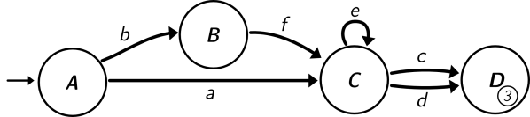
Figure 1. Call graph representing a program with four functions: $A$, $B$, $C$, and $D$. Each edge represents a function call from a certain call site in the program, and is marked with a unique label.

Call strings provide the context that is relevant for context-sensitive holes. Ideally, the tuning should find the optimal value for each call string in $\mathit{CS}_{i}$ leading to the $i$th hole. However, in Example 3.1 we see that there can be infinitely many call strings, which means that we would have infinitely many decision variables to tune. Therefore, we wish to partition the call strings into equivalence classes, and tune each equivalence class separately. This leads to the question of how to choose the equivalence relation.

One possible choice of equivalence relation is to consider two call strings that have an equal suffix (that is, an equal ending) as being equal. We can let the length of the suffix be $d$, where $d$ is the context depth of the hole:

Example 3.2.

Let $\sim_{i}$ be an equivalence relation defined on each set $\mathit{CS}_{i}$, such that:

$$s_{1}\sim_{i}s_{2}\ \text{iff}\ \text{suffix}_{\delta{i}}(s_{1})=\text{suffix}_{\delta{i}}(s_{2})\text{, }s_{1},s_{2}\in\mathit{CS}_{i}$$

where $\text{suffix}_{d}(s)$ returns the last $d$ labels of a call string $s$, or all of the labels if the length of the string is less than $d$. We choose a canonical representation from each equivalence class as the result from the $\text{suffix}_{d}$ function. The call strings from Example 3.1 have the following canonical representations (that is, unique results after applying $\text{suffix}_{3}$ to the call strings):

$$\mathit{ac},\mathit{aec},\mathit{eec},\mathit{ad},\mathit{aed},\mathit{eed},\mathit{bfc},\mathit{fec},\mathit{bfd},\mathit{fed}$$

Note that the canonical representations are suffixes of call strings but not always call strings by strict definition, as they do not always start in a start vertex $v_{s}\in S$. We call these canonical representations context strings. ∎

While the equivalence relation in Example 3.2 at least gives an upper bound on the number of decision variables to tune, it may still result in a large number of equivalence classes. Limiting the number of recursive calls that are considered results in a more coarse-grained partitioning:

Example 3.3.

Consider the equivalence relation $\sim_{i}^{r}$, which is like $\sim_{i}$ from Example 3.2, but where we consider at most $r$ repetitions of any label, for some parameter $r$. That is, if a string contains more than $r$ repetitions of a label, then we keep the $r$ rightmost occurrences. For example, using $r=1$ in the call strings of Example 3.1 yields the $8$ context strings:

$$\mathit{ac},\mathit{aec},\mathit{ad},\mathit{aed},\mathit{bfc},\mathit{fec},\mathit{bfd},\mathit{fed}$$

Note that compared to the context strings in Example 3.2, we have filtered out $\mathit{eec}$ and $\mathit{eed}$ as they include more than $1$ repetition of the label $e$. For example, this means that the two call strings $\mathit{aec}$ and $\mathit{aeec}$ belongs to the same equivalence class, namely the class represented by the context string $\mathit{aec}$. ∎

Using the definition of context strings, we can finally define what we mean by context-sensitive holes. Given some equivalence relation $\sim$, a base hole is expanded (by the compiler) into $c$ number of context holes, where $c$ is the number of equivalence classes (i.e., the number of context strings) under the relation $\sim$. If $\delta(i)=0$, then the hole is global, and $c=1$. In Example 3.2, there are $10$ context holes, and in Example 3.3 there are $8$. Thus, the choice of the equivalence relation influences the number of decision variables to tune: few equivalence classes give fewer variables to tune and potentially a shorter tuning time, while more classes might increase the tuning time, but give better performance of the resulting program.

3.2. Graph Coloring for Tracking Contexts

Each time a context-sensitive hole is used, we need to decide which equivalence class the current call string belongs to, in order to know which value of the hole to use. The challenge is to introduce tracking and categorization of call strings in the program with minimum runtime overhead. A naive approach is to explicitly maintain the call string during runtime. However, this requires book keeping of auxiliary data structures and potentially makes it expensive to decide the current context string. This section describes an efficient graph coloring scheme that leaves a color trail in the call graph, thereby implicitly maintaining the call history during runtime of the program. We first discuss the underlying equivalence relation that the method implements (Section 3.2.1), and then divide our discussion of the graph coloring into two parts: complete programs (Section 3.2.2) and separately compiled library code (Section 3.2.3).

3.2.1. Equivalence Relation

The equivalence relation that the graph coloring method implements is an approximation of the $\sim_{i}^{1}$ relation of Example 3.3. The difference is that we do not track the call string beyond a recursive (including mutually recursive) call. This is because a recursive call overwrites the call history in graph coloring, as we will see in Section 3.2. The context strings for the call strings from the previous section are:

$$\mathit{ac},\mathit{ec},\mathit{ad},\mathit{ed},\mathit{bfc},\mathit{bfd}$$

Compared to the context strings in Example 3.3, the strings $\mathit{aed}$ and $\mathit{fed}$ are merged into $\mathit{ed}$, and the strings $\mathit{aec}$ and $\mathit{fec}$ are merged into $\mathit{ec}$. A consequence is that, for instance, the call strings $\mathit{bfed}$ and $\mathit{aed}$ belong to the same equivalence class, namely the class represented by $\mathit{ed}$.

Algorithm 1 describes how to explicitly compute the context strings for the $i$th hole. The recursive sub-procedure ContextStringsDFS traverses the graph in a backwards depth-first search manner. It maintains the current vertex $v$ (initially $\eta(i)$), the current string $s$ (initially the empty string $\epsilon$), the set of visited vertices $U$ (initially $\varnothing$) and the remaining depth $d$ (initially $\delta(i)$).

Algorithm 1 Algorithm for computing the context strings of a hole.

Input Call graph $G=(V,E,L,S,H)$, index $i$ of the base hole.
Output Set of context strings of the hole.

1:procedure ContextStrings($G$,$i$)

2:     procedure ContextStringsDFS($v$, $s$, $U$, $d$)

3:         if $d=0\lor\text{inc}(G,v)=\varnothing\lor v\in U$ then return $\{s\}$

4:         else

5:              $\mathit{CS}\leftarrow\bigcup\limits_{(v_{p},v,l)\in\text{inc}(G,v)}\textsc{ContextStringsDFS}(v_{p},s\oplus l,U\bigcup\{v\},d-1)$

6:              if $v\in S$ then return $\mathit{CS}\bigcup\{s\}$

7:              else return $\mathit{CS}$                             

8:     return ContextStringsDFS($\eta(i)$, $\epsilon$, $\varnothing$, $\delta(i)$)

Line 3 returns a singleton set if the depth is exhausted, if the set of incoming edges to $v$ is empty, or if $v$ is visited. The function $\text{inc}(G,v)$ returns the set of incoming edges to vertex $v$ in $G$. Line 5 recursively computes the context strings of the preceding vertices of $v$, and takes the union of the results. The $\oplus$ operator adds a label to a string. Lines 6–7 return the final result. If the current vertex $v$ is a start vertex, then the current string $s$ is a context string starting in $v$, and is therefore added to the result. Otherwise, we return the result of the recursive calls.

3.2.2. Coloring a Complete Program

In the case of a complete program, the program has a single entry point, for instance, a main function where the execution starts. We will now walk through a number of examples, showing how graph coloring works conceptually.

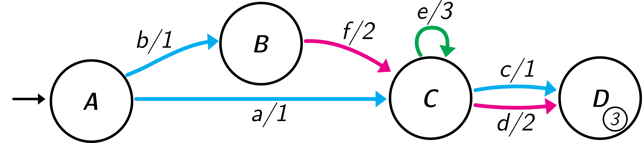
(a) Initial state of the call graph when performing graph coloring: all vertices are white, and each edge is colored so that the colors of the incoming edges for each node are different. For readability on a black and white rendering of the figure, we mark each edge with an integer representing the color in addition to coloring the edge ($1$ for blue, $2$ for magenta, and $3$ for green).

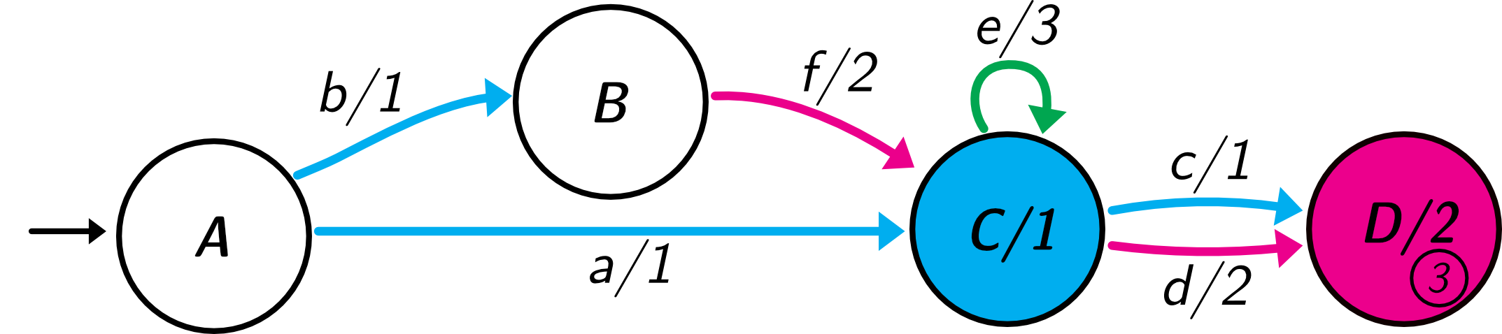
(b) State of the call graph after the call string $\mathit{ad}$ is taken. For readability, for each non-white node we write the integer representing the color in the vertex in addition to coloring it.

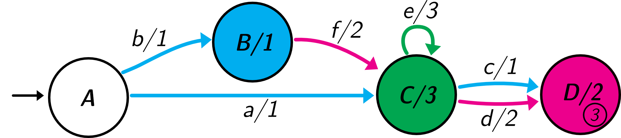
(c) State of the call graph after the call string $\mathit{bfed}$ is taken. Because of the recursive call in $C$, we cannot trace the calls further backward from $B$. The current context string is therefore $ed$.

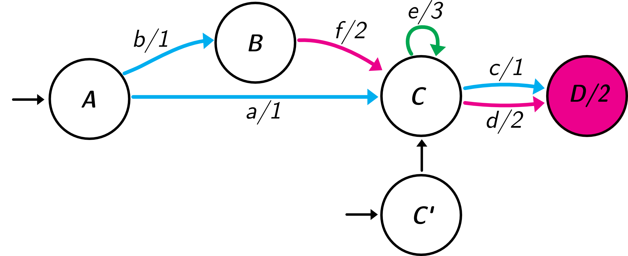
(d) A call graph with several entry points. Node $C^{\prime}$ is a sentinel vertex that forwards external calls to the internal vertex $C$. The call string $\mathit{ac}$ has been taken, immediately followed by call string $c$. The current context string is $c$.

Figure 2. Conceptual illustration of how the call history is maintained by coloring the call graph during runtime.

Example 3.4.

Figure 2(a) shows the initial coloring state of the call graph in Figure 1. For instance, the vertex $C$ has three incoming edges (with colors blue ($1$), magenta ($2$), and green ($3$)), while $D$ has two (blue and magenta). Note that we can reuse a given color for several edges, as long as each vertex does not have two incoming edges with the same color. For instance, the edges labeled $a$ and $b$ are both blue. ∎

Algorithm 2 describes the update to the coloring when an edge is traversed in the call graph.

Algorithm 2 Traversing an edge.

Input A call graph $G=(V,E,L,S,H)$, coloring functions $c_{V}$ and $c_{L}$, and traversed edge $(v_{1},v_{2},l)\in E$.
Output Modified coloring function $c_{V}^{\prime}$.

1:procedure TraverseEdge($G,c_{V},c_{L}$, $(v_{1},v_{2},l)$)

2:     $c_{V}\leftarrow\left(c_{V}\setminus\{v_{2}\mapsto c_{V}(v_{2})\}\right)\bigcup\{v_{2}\mapsto c_{L}(l)\}$ $\triangleright$ Overwrite previous mapping of $v_{2}$ in $c_{V}$

3:     return $c_{V}$

Line 2 updates the color of the destination vertex to the color of the label of the edge being traversed.

Example 3.5.

Figure 2(b) shows the state of the call graph after the call string $\mathit{ad}$ is taken, and Figure 2(c) shows the state after the call string $\mathit{bfed}$ is taken. ∎

When the value of a hole is used during runtime of the program, we check the current context by following the colors of the vertices and edges backwards in the graph. The tracing stops when we reach the depth of the hole, when we reach a white vertex, or when we detect a cycle.

Example 3.6.

To determine the current context string in Figure 2(b), we first inspect the color of $D$ (magenta), which means that $d$ is the last label in the string. Next, we see that $C$ is blue, so $C$ was called by $A$, thus $a$ is the second to last label. The color of $A$ is white, so we stop the tracing. Thus, the context string is $ad$. ∎

Example 3.7.

Similarly, in Figure 2(c) we determine that the last two labels are $d$ and $e$. Since $C$ called itself via $e$, we have detected a cycle. Thus, the context string is $ed$. ∎

3.2.3. Code Libraries

In contrast to a complete program, a separately compiled code library may have several entry points, namely, the publicly exposed functions. Further, each entry point may have incoming edges from internal calls within the library. This poses a problem for the coloring scheme described thus far, illustrated in the following example.

Example 3.8.

Assume that vertex $C$ in Figure 2(a) also is an entry point, along with vertex $A$. Then the set of context strings listed in Section 3.2.1 is extended with $\mathit{c}$ and $\mathit{d}$. The reason for this is that a call directly to $C$ can result in the path $c$ or path $d$, without visiting any other edges. Further, assume that the call string $\mathit{ac}$ has been taken immediately before a call to $C$ is made and the call string $c$ is taken. Then the coloring state of the graph would be like in Figure 2(b), if we follow the coloring scheme described thus far. From this state, we cannot determine whether the current context string is $\mathit{ac}$ or $c$. ∎

A possible solution to this problem is shown in Figure 2(d). For each library node ($C$ in this example), we add an sentinel vertex (noted with a prime) which directly connects to the original entry point of the library. If a call is via an sentinel vertex, the next vertex is colored white. Hence, it is possible to distinguish between if the call is coming from the library entry point or from another vertex in the graph.

3.3. Implementation of Graph Coloring

The input to the program transformations is a program $p$ with holes, as well as the path to the tune file. The output is a transformed program $p_{t}$ that performs graph coloring, and where each base hole in $p{}$ has been replaced by code that statically looks up a value depending on the current context. We discuss the program transformations in Section 3.3.1, and analyze the runtime overhead of the transformed program in Section 3.3.3.

3.3.1. Program Transformations

During compile-time, we build a call graph $G$ as defined in Section 3.1. A key idea is that we do need to maintain the call graph during runtime of the program; it is only used for analysis during the program transformations.

In the transformed program, we introduce for each vertex $v\in V^{\prime}$, an integer reference $r_{v}$ whose initial value is $0$ (white).

The TraverseEdge procedure in Algorithm 2 is then implemented as a transformation. Immediately before a function call from $v_{1}$ to a function $v_{2}$, where $(v_{1},v_{2},l)\in E^{\prime}$, we introduce an update of the reference $r_{v_{2}}$ to the color (i.e., integer value) that the edge $(v_{1},v_{2},l)$ is assigned to.

Finally, determining the current context string, as informally described in Examples 3.6 and 3.7 also requires a program transformation, which we call context expansion. In context expansion, we replace each base hole in the program with code that first looks up the current context string, and thereafter looks up the value of the associated context hole. Determining the current context string for a hole of depth $d$ requires checking the values of at most $d$ integer references. For example, if the following declaration of a base hole exists in vertex $D$ in Figure 1:

⬇

1hole (Boolean {default = true, depth = 3})

then we replace it by the following program code:

⬇

1switch deref $r_{D}$

2case 1 then

3 switch deref $r_{C}$

4 case 1 then <lookup $\mathit{ac}$>

5 case 2 then <lookup $\mathit{bfc}$>

6 case 3 then <lookup $\mathit{ec}$>

7 end

8case 2 then

9 switch deref $r_{C}$

10 case 1 then <lookup $\mathit{ad}$>

11 case 2 then <lookup $\mathit{bfd}$>

12 case 3 then <lookup $\mathit{ed}$>

13 end

14end

where deref reads the value of a reference, each $r_{v}$ is the reference storing the color of function $v$, and each <lookup$\phantom{s}s$> is code that looks up the value for the context hole associated with the context string $s$. In the final tuned program, each <lookup $\phantom{s}s$> is simply a static value: the value that has been tuned for context $s$ (tuned compilation, see Section 6). During tuning of the program, each <lookup $\phantom{s}s$> is an access into an array that stores the values of the context holes contiguously. This array is read as input to the program via the tune file, so that the program does not have to be re-compiled during tuning (see Section 6 for more details). Note that a global hole (depth $0$) can be seen as having one context string, namely the empty string, and thus does not need any switch statement.

3.3.2. Adaption to Parallel Execution

In a parallel execution setting, there might be more than one active call string during each given time in the program. We make an adaption to the program transformation in order to handle a fixed number of threads $T$. Instead of introducing one reference per (relevant) function, we introduce an array with $T$ number of references per (relevant) function. Each thread $t$ is assigned an array index $t_{i}$. Each thread uses the references at index $t_{i}$ only. In this way, we maintain up to $T$ active context strings simultaneously. If a thread pool is used, then the size of the thread pool needs to be known at compile-time. Otherwise, the transformation works as described in Section 3.3.1.

3.3.3. Runtime Overhead in the Resulting Program

As a baseline for runtime overhead, consider the original program $p{}$ where each base hole is replaced by its default value (default compilation, see Section 6): we call this program $p_{\mathit{def}}$. The overhead of the transformed program $p_{t}$ compared to $p_{\mathit{def}}{}$ when the number of threads $T=1$, includes initializing at most one integer reference per function. The program $p_{t}$ performs at most one reference update per function call. Moreover, $p_{t}$ performs at most $d$ number of matches on references in switch statements each time it uses the value of a hole, where $d$ is the depth of the hole. The underlying compiler can transform the switch statements into an indexed lookup table. This lookup table is compact by construction, as we use contiguous integers as values representing colors. When $T>2$, then $p_{t}$ introduces at most one array of references per function, and each reference update and reference read includes an indexing into an array.

4. Static Dependency Analysis

This section discusses static dependency analysis. The goal is to detect holes that can be tuned independently of each other. This information is later used during tuning in order to reduce the search space. Section 4.1 motivates the need of dependency analysis and provides intuition, Section 4.2 makes necessary definitions that are used in Section 4.3, which describes the details of the dependency analysis. Finally, Section 4.4 describes how the program is instrumented given the result of the dependency analysis.

4.1. Motivation and Running Example

Consider the following $k$-nearest neighbor ($k$-NN) classifier, which will be our running example in this section:

⬇

38let knnClassify = lam k: Int. lam data: [([Int],Label)]. lam query: [Int].

39 -- Step 1: compute the distance to each point in the data set

40 let dists: [(Int,Label)] = map (lam d: ([Int],Label). --*\label{l:knn-dists-start}*--

41 (euclideanDistance query d.0, d.1)

42 ) data --*\label{l:knn-dists-end}*--

43 in

44 -- Step 2: sort the distances in ascending order

45 let sortedDists: [(Int,Label)] = sort (

46 lam d1: (Int,Label). lam d2: (Int,Label). subi d1.0 d2.0

47 ) dists

48 in

49 -- Step 3: return the most common label among the k nearest neighbors

50 let kNearest: [(Int,Label)] = subsequence sortedDists 0 k in --*\label{l:knn-subsequence}*--

51 mostCommonLabel kNearest

The classifier takes three arguments: the parameter k of the algorithm; the data set, which is a sequence of tuples $(d,l)$, where $d$ is a data point (representing an integer vector) and $l$ is the class label; and the query data point, whose class label we want to decide.

The algorithm has three steps. In the first step, we compute the pairwise distances between the query and each point in the data set, in this example using Euclidean distance. In step two, we sort the pairwise distances. The first argument to the function sort is the comparison function, which in this case computes the difference between two distances. In the last step, we extract the $k$ nearest neighbors by taking the $k$ first elements in the sorted sequence sortedDists. Finally, we assume that the mostCommonLabel function returns the most frequent label in a sequence of labels, so that the query point is classified to the most common class among its neighbors.

Now, assume that the $k$-NN classifier implicitly uses three holes. The first hole, $h_{\text{seq}}$, is for deciding the underlying data structure for the sequences. In the Miking core language, a sequence can either be represented by a cons list, or a Rope (Boehm et al., 1995). We can use a Boolean hole to choose the representation when creating the sequence, by either calling the function createList or createRope. The second hole, $h_{\text{map}}$, chooses between sequential or parallel code in the map function, see Example 2.3. Finally, the third hole, $h_{\text{sort}}$, chooses between two sorting algorithms depending on an unknown threshold value, see Example 2.1.

When tuning the classifier, these three choices need to be taken into consideration. If the program is seen as a black box, then an auto tuner needs to consider the combination of each of these choices. In this small example, we quickly see that while some choices are indeed necessary to explore in combination, others can be explored in isolation. Choices that must be explored together, called dependent choices, are for instance: (i) the underlying sequence representation and the map function ($h_{\text{seq}}$ and $h_{\text{map}}$); and (ii) the underlying sequence representation and the sort function ($h_{\text{seq}}$ and $h_{\text{sort}}$). In both cases, this is because the sequence representation affects the execution time of the operations performed on the sequence in the respective function. On the other hand, the sort function and the map function do not need to be explored in combination with each other: the holes $h_{\text{map}}$ and $h_{\text{sort}}$ are independent of each other. Regardless of what choice is made in the map function (sequential or parallel), the result of the function is the same, which means that the sort function should be unaffected.

With knowledge about independencies, an auto tuner can use the tuning time in a more intelligent way, as it does not need to waste time exploring unnecessary combinations of holes. The remainder of this section describes how we can automatically detect (in-)dependencies such as the examples discussed here, using static analysis.

4.2. Definitions

Before discussing the details of the dependency analysis, we need to define the entities that constitute dependency: measuring points and dependency graphs.

4.2.1. Measuring Points

Intuitively, two holes are independent if they affect the execution time of disjoint parts of the program. That is, we want to find the set of subexpressions of the program whose execution times are affected by a given hole. There are often many such subexpressions. For instance, the complete knnClassify in Section 4.1 is a subexpression whose execution time depends on three holes: $h_{\text{seq}}$, $h_{\text{map}}$, and $h_{\text{sort}}$. Moreover, the subexpression on Lines LABEL:l:knn-dists-start–LABEL:l:knn-dists-end (the computation of dists) in knnClassify depends on $h_{\text{seq}}$ and $h_{\text{map}}$. So how do we choose which subexpressions that are relevant in the dependency analysis?

Clearly, it is not useful to consider too large subexpressions of the program. This is because two holes $h_{1}$ and $h_{2}$ may affect a large subexpression $e$, even though they in reality only affect smaller, disjoint subexpressions $e_{1}$ and $e_{2}$, respectively, where $e_{1}$ and $e_{2}$ are subexpressions of $e$. Therefore, we want to find small subexpressions whose execution time depends on a given hole. We exemplify the type of expressions we are interested in for knnClassify in Example 4.1, before going into details.

Example 4.1.

Assume that the map function is given by Example 2.3, and the sort function is given by Example 2.1. A small subexpression affected by $h_{\text{map}}$ is Line LABEL:l:par-ite in map (the if-then-else expression), because which branch is taken is decided by the hole par. Similarly, the if-then-else expression on Lines LABEL:l:sort-ite-1–LABEL:l:sort-ite-2 in sort is a small subexpression affected by $h_{\text{sort}}$. These two subexpressions are also affected by $h_{\text{seq}}$, because the execution times of the branches depend on the underlying sequence representation. Furthermore, Line LABEL:l:knn-subsequence in knnClassify is a minimal subexpression affected by $h_{\text{seq}}$, because the execution time of subsequence also depends on the underlying sequence representation. ∎

We call these small subexpression whose execution time depends on at least one hole a measuring point. The rationale of the name is that we measure the execution time of these subexpressions by using instrumentation (see Section 4.4). The Miking language, being a core language, consists of relatively few language constructs; any higher-order language implemented on top of Miking will compile down to this set of expressions. The type of expressions that construct measuring points are either:

1. a match statement (including if-then-else expressions); or

2. a call to a function f x, where f is either a built-in function (such as subsequence), or user-defined.

Section 4.3 clarifies under which circumstances these expressions are measuring points. Other types of expressions in Miking, such as lambda expressions, constants, records, and sequence literals, are not relevant for measuring execution time.

4.2.2. Dependency Graph

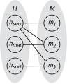
Figure 3. Dependency graph for the knnClassify function in Section 4.1. The set $H$ is the set of holes (the choice of sequence representation, choice of sequential or parallel map, and the choice of sorting function, respectively). The set $M$ is the set of measuring points, where $m_{1}$ is Line LABEL:l:knn-subsequence of knnClassify, point $m_{2}$ is Line LABEL:l:par-ite of map, and $m_{3}$ is Lines LABEL:l:sort-ite-1–LABEL:l:sort-ite-2 of sort.

We now define dependency graphs. Given a program $p{}$ with a set of context holes $H{}$, and a set of measuring points $M{}$, its dependency graph is a bipartite graph $(H{},M{},E)$. There is an edge $(h,m)\in E$, $h\in H$, $m\in M$, iff the hole $h$ affects the execution time of $m$.

Example 4.2.

A (partial) dependency graph of knnClassify is given by Figure 3. It is partial because there are more measuring points in the functions mostCommonLabel and pmap (because they contain sequence operations, whose execution times depend on $h_{\text{seq}}$), but these functions are omitted for brevity. ∎

The dependency graph encodes the dependencies among the program holes. For instance, in Figure 3, we see that $h_{\text{seq}}$ and $h_{\text{map}}$ are dependent, because they both affect $m_{2}$, while $h_{\text{map}}$ and $h_{\text{sort}}$ are independent, because they have no measuring point in common.

4.3. Dependency Analysis

The goal of the dependency analysis is to compute the dependency graph of a given program.

4.3.1. 0-CFA analysis

The backbone of the dependency analysis is $0$-CFA analysis (Nielson et al., 1999). We extend standard $0$-CFA analysis, which tracks data-flow of functions, to additionally track data-flow of holes. The result is that we compute for each subexpression in the program the set of holes that affect the value of the subexpression.

Standard data-flow rules apply. The first two columns of Table 1 shows the result of the data-flow analysis for a few example subexpressions from knnClassify. We denote the data dependency of a subexpression by the set of holes whose value the subexpression depends on. In the first row, the variable query depends on $h_{\text{seq}}$ because the variable refers to a sequence whose representation is decided by $h_{\text{seq}}$. Second, the if-then-else expression from the map function depends on both $h_{\text{seq}}$ and $h_{\text{map}}$, because the condition of the if-then-else depends on $h_{\text{map}}$, and the result of the subexpression is again a sequence dependent on $h_{\text{seq}}$. In the third row, the variable dists also depends on both $h_{\text{seq}}$ and $h_{\text{map}}$, because the variable refers to the result of the map function. In the fourth row, Lines LABEL:l:sort-ite-1–LABEL:l:sort-ite-2 in Example 2.1 depends on all three holes. It depends on $h_{\text{sort}}$ because the condition of the if-then-else depends on $h_{\text{sort}}$. It depends on $h_{\text{seq}}$ and $h_{\text{map}}$ because the branches of the if-then-else manipulate the sequence referred to by dists. Finally, the call to subsequence also depends on all holes, because the built-in function subsequence returns a sequence that will have the same data dependency as its input sequence, sortedDists.

Table 1. Result of the dependency analysis for a subset of the subexpressions in knnClassify, using Examples 2.1 and 2.3 as implementations of sort and map, respectively. Columns $2$–$3$ and $4$–$5$ show the data dependency and the execution time dependency of each subexpression, for a program without and with annotations, respectively. We see that without the annotation, the analysis concludes that all three holes are execution time dependent, while the version with annotations results in the dependency graph in Figure 3.

	Without annotations		With annotations
Subexpression	Data dep.	Exe. dep.	Data dep.	Exe. dep.
query	$\{h_{\text{seq}}\}$	$\varnothing$	$\{h_{\text{seq}}\}$	$\varnothing$
if par then ... else ...	$\{h_{\text{seq}},h_{\text{map}}\}$	$\{h_{\text{seq}},h_{\text{map}}\}$	$\{h_{\text{seq}}\}$	$\{h_{\text{seq}},h_{\text{map}}\}$
dists	$\{h_{\text{seq}},h_{\text{map}}\}$	$\varnothing$	$\{h_{\text{seq}}\}$	$\varnothing$
Lines LABEL:l:sort-ite-1–LABEL:l:sort-ite-2 in Example 2.1	$\{h_{\text{seq}},h_{\text{map}},h_{\text{sort}}\}$	$\{h_{\text{seq}},h_{\text{map}},h_{\text{sort}}\}$	$\{h_{\text{seq}}\}$	$\{h_{\text{seq}},h_{\text{sort}}\}$
subsequence sortedDists 0 k	$\{h_{\text{seq}},h_{\text{map}},h_{\text{sort}}\}$	$\{h_{\text{seq}},h_{\text{map}},h_{\text{sort}}\}$	$\{h_{\text{seq}}\}$	$\{h_{\text{seq}}\}$

Recall that we are interested in subexpressions whose execution time (not value) depends on holes: these are the measuring points of the program. Luckily, we can incorporate the analysis of measuring points into the $0$-CFA, by using the data-flow information of the holes. Besides data dependency, we introduce another kind of dependency: execution time dependency. A subexpression with a non-empty execution time dependency is a measuring point. There are two kinds of expressions that may give rise to execution time dependency, i.e., measuring points: match expressions, and calls to functions.

Match Expressions.

Given a match expression e on the form match e1 withpat then e2 else e3, the following two rules apply: (1) If e1 is data-dependent on a hole $h$, then e is execution time-dependent on $h$; and (2) If e2 executes (directly or via a function call) another subexpression that is execution time-dependent on a hole $h$, then e is also execution time-dependent on $h$, and the same applies for e3. The justification of rule 1 is that if the decision of which branch to take depends on a hole, then the execution time of the match expression depends on the hole. The justification of rule 2 is that the execution time of the whole subexpression e should include any execution time dependencies of the individual branches.

The third column of Table 1 shows execution time dependencies of some subexpressions in knnClassify. Rows 2 and 4 are match expressions. Note that in the Miking core language, an if-then-else expression is syntactic sugar for a match expression where pat is true. The conditions of the match expressions depend on $h_{\text{map}}$ and $h_{\text{sort}}$, respectively, thus these holes are included in the execution time dependencies. The branches of each subexpression perform sequence operations, which will be measuring points dependent on $h_{\text{seq}}$. Thus, the execution time of the match expressions also depends on $h_{\text{seq}}$. The dependency on row 4 also includes $h_{\text{map}}$, because the input sequence, dists, has a data dependency on $h_{\text{map}}$.

Function calls.

If the expression e is the result of an application of a built-in function, then custom rules apply for each built-in. For instance, for the expression subsequence s i j, if the sequence s is data-dependent on a hole $h$, then e is execution time-dependent on $h$. The subsequence expression in the last row of Table 1 has the same execution time dependency as its data dependency, by following this rule.

In addition, for all function calls e on the form e1e2, if e1 is data-dependent on a hole $h$, then e is execution time-dependent on $h$. As a simple example, the function call (if h then f else g) x is a measuring point, given that h is data-dependent on some hole. In other words, since the left hand side of the application is determined by a hole, the execution time of the function call depends on a hole.

Note that the function call on Lines LABEL:l:knn-dists-start–LABEL:l:knn-dists-end in knnClassify does not constitute a measuring point, even though its execution time depends on $h_{\text{seq}}$ and $h_{\text{map}}$. The reason is that the function map itself is not data-dependent on a hole. The relevant execution times of the map functions are already captured by measuring points within the map function.

4.3.2. Call Graph Analysis

The $0$-CFA analysis finds the set of measuring points of the program and attaches an initial set of dependencies to each measuring point. Some dependencies, however, are not captured in the $0$-CFA analysis. Namely, if a measuring point $m_{1}$ executes another measuring point $m_{2}$, then the holes that affect $m_{2}$ also affect $m_{1}$. For instance, the expression if par then pmap f s else smap f s executes any measuring points within the pmap and smap function. We perform another analysis step that analyzes the call graph of the program, in order to find the set of measuring points that each measuring point executes. This analysis step does not introduce any new measuring points, but it adds more dependencies (edges in the dependency graph).

4.3.3. False Positives and Annotations

As we have seen so far, the dependencies (both for data and execution time) on some subexpressions in Table 1 are unnecessarily large. For instance, the value of the subexpression on row 2 should intuitively not depend on $h_{\text{map}}$. After all, whether the map is performed in parallel or sequentially does not affect the final result. In other words, the data dependency on $h_{\text{map}}$ on row 2 is a false positive.

The result of false positives on data dependencies is that some execution time dependencies may also be unnecessarily large. As we see in Table 1, the false positive on $h_{\text{map}}$ on row 2 propagates to the data dependency of row 3 (dists), which in turn affects the execution time dependencies of rows 4 and 5.

While it is in general hard for a compiler to detect, for instance, that parallel and sequential code gives the same end result, or that two sorting functions are equivalent, this information is typically obvious for a programmer.

Therefore, we introduce the option to add annotations to a program to reduce the number of false-positive dependencies. The annotation states the set of variables that a match expression is independent of, and is added directly after a match expression using the keyword independent.

For instance, replacing Line LABEL:l:par-ite in Example 2.3 with independent (if par then pmap f s else smap f s) par states that the value of the match expression is independent of the variable par. More variables can be included in the set by nesting several independent annotations, e.g. independent (independent<e> x) y.

By incorporating this information in the analysis, the data dependency on the independent set is ignored for the match expression. Columns $4$–$5$ in Table 1 show the result of the analysis given that the match expressions on rows 2 and 4 have been annotated to be independent of the variables par and threshold, respectively. We see that the execution time dependencies now match the dependency graph in Figure 3. Row 2 in Table 1 corresponds to $m_{2}$, row 4 corresponds to $m_{3}$, and row 5 corresponds to $m_{1}$.

4.3.4. Context-Sensitive Measuring Points

A property of $0$-CFA is that it does not include context information for the data-flow, unlike $k$-CFA for $k>0$. While we are limited to $0$-CFA for efficiency reasons, it is necessary to consider the contexts of context-sensitive holes. Therefore, we consider the context strings (see Section 3) during the dependency analysis.

As an example, consider the map function in Example 2.3. Assume that it is called from two locations, so that there are two possible call strings for the hole par; $s_{1}$ and $s_{2}$. During analysis of the measuring point on Line LABEL:l:par-ite, we conclude that the execution time depends either on the context hole associated with $s_{1}$, or the one associated with $s_{2}$, but not both. This is taken into account during instrumentation of the program, see Section 4.4.

4.4. Instrumentation

The instrumentation is a program transformation step, where the input is the program $p$ and the dependency graph $G=(H{},M{},E)$. The output is an instrumented program $p_{I}$ that collects execution time information for each measuring point. Section 4.4.1 introduces three challenges when designing the instrumentation. In Section 4.4.2, we present the proposed design and clarify how the design addresses the identified challenges.

4.4.1. Challenges

Assume that we wish to instrument the measuring point in row 2 in Table 1 on page 1: if parthen pmap f s else smap f s. A naive approach is to save the current time before and after the expression has been executed, and then record the elapsed time after the expression has been executed.

However, there are a number of problems with this simple solution. First, the measuring point can execute another measuring point. In this specific case, it executes any measuring points within the pmap or smap functions. If we do not keep track of whether a measuring point executes within another one, we will count some execution times several times, which gives an inaccurate total execution time of the program. Second, this simple instrumentation approach does not allow for tail-call optimizations. The reason is that after the transformation of the program, some operations are performed after the execution of the measuring point. The result is that a recursive call within the measuring point will no longer be in tail position. The third challenge has to do with context-sensitivity. For instance, assume that map in Example 2.3 is called from two locations. The instrumented code must then consider these two calling contexts when recording the execution of the measuring point.

4.4.2. Solution

The instrumentation introduces a number of global variables and functions in the program, maintaining the current execution state via a lock mechanism. Moreover, every measuring point is uniquely identified by an integer. In particular:

• The variable lock stores the identifier of the measuring point that is currently running, where the initial value $0$ means that no measuring point is running. Note that we do not mean a lock for parallel execution; we can still execute and measure parallel execution of code.

• The array s of length $|M|$, where s$[i]$ stores the latest seen start time of the $i$th measuring point.

• The array log of length $|M|$, where log$[i]$ stores a tuple $(T,n)$ where $T$ is the accumulated execution time, and $n$ is the number of runs, of the $i$th measuring point.

• The function acquireLock takes an integer $i>0$ (a unique identifier of a measuring point) as argument, and is called upon entry of a measuring point. If the lock equals $0$, then the function sets lock to $i$, and writes the current time to ${\leavevmode\lstinline{{\lst@@@set@language\lst@@@set@numbers\lst@@@set@frame\lst@@@set@rulecolor\lst@@@set@numbers\lst@@@set@language\footnotesize{\@listingGroup{ltx_lst_identifier}{s}}}}}[i]$. Otherwise, that is, if the lock is already taken, the function does nothing.

• The function releaseLock also takes an integer identifier $i>0$ as argument, and is called when a measuring point exits. If the lock equals $i$, then the function sets lock to $0$, and adds the elapsed execution time to the global log. If the lock is taken by some other measuring point, the function does nothing.

After the instrumented program is executed, the array log stores the accumulated execution time and the number of runs for each measuring point.

As a result, the measuring point in row 2 in Table 1 is replaced by the following lines of code:

⬇

1acquireLock $\mathit{i}$; --*\label{l:instr-1}*--

2let v = if par then pmap f s else smap f s in --*\label{l:instr-2}*--

3releaseLock $\mathit{i}$; --*\label{l:instr-3}*--

4v

The lock design addresses the first of the identified challenges: to keeping track of whether a measuring point is executed within another one. Because only one measuring point can possess the lock at any given moment, we do not record the execution if one executes within another. Thus, the sum of the execution times in the log array never exceeds the total execution time of the program.

We now consider the second challenge: allowing for tail-call optimization. For a measuring point with a recursive call f x in tail position, for instance if <$\mathit{cond}$> then <$\mathit{basecase}$> else f x, the call to releaseLock is placed in the base case only, so that the recursive call remains in tail position:

⬇

1acquireLock $\mathit{i}$;

2if <$\mathit{cond}$> then

3 let v = <$\mathit{basecase}$> in

4 releaseLock $\mathit{i}$;

5 v

6else f x

There can be more than one call to releaseLock in each base case, because of measuring points in mutually recursive functions. The instrumentation analyzes the (mutually) recursive functions within the program and inserts the necessary calls to releaseLock in the base cases of these functions.

The third challenge, dependency on context-sensitive holes, is addressed similarly as in Section 3.3.1. Consider again the measuring point if par then pmap f s else smap f s in within the map function, and assume that there are two possible calls to map. The measuring point is assigned a different identifier depending on which of these contexts is active. The identifier is found by a switch expression of depth 1, reading the current color of the map function. If there is only one call to map, then the identifier is simply an integer, statically inserted into the program.

5. Dependency-Aware Tuning

In contrast to standard program tuning, dependency-aware tuning takes the dependency graph into account to reduce the search space of the problem. This section describes how to explore this reduced search space, and how to find the expected best configuration given a set of observations.

5.1. Reducing the Search Space Size

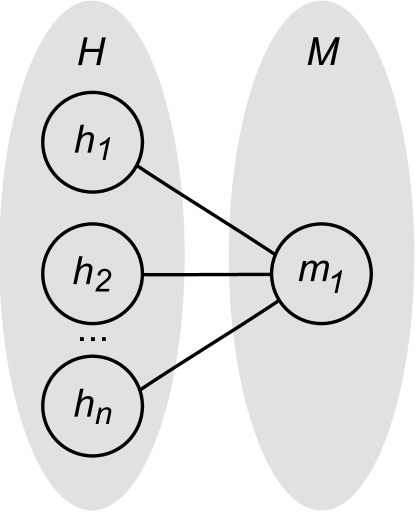
(a) Dependency graph of a program with fully dependent holes. All $2^{n}$ possible combinations need to be taken into consideration when tuning.

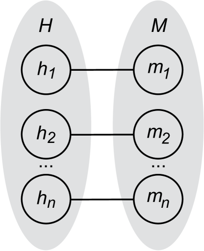
(b) Dependency graph of a program with fully independent holes. It is enough with $2$ program runs to exhaust the search space if fine-grained instrumentation of each measuring point is used.

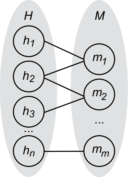
(c) Dependency graph that is neither fully dependent nor fully independent. The number of required program runs with instrumentation is $2^{r}$, where $r$ is the maximum number of holes affecting any given measuring point.

Figure 4. Possible dependency graphs for a program with $n$ holes of Boolean type. In all cases, there are $2^{n}$ number of possible configurations. However, the more independence, the fewer of these configurations need to be considered when tuning.

In standard program tuning (without dependency analysis), each hole needs to be tuned in combination with every other hole, which means that the number of configurations to consider grows exponentially with the number of holes.

Example 5.1.

Consider a program with $n$ Boolean holes, which has a search space of size $2^{n}$. With no dependency analysis, we may view the program as consisting of one measuring point, affected by all the holes in the program. This corresponds to the dependency graph in Figure 4(a). If exhaustive search is used, then $2^{n}$ program runs are required to find the optimal configuration. ∎

Dependency analysis finds the fraction of the total number of configurations that are relevant to evaluate during tuning, as illustrated in Examples 5.2 and 5.3.

Example 5.2.

Consider the program from Example 5.1. Figure 4(b) shows a dependency graph where all the holes are completely independent, so that each measuring point is affected by exactly one hole. If instrumentation is used, we collect the execution time for each measuring point in isolation. In this case, it is enough to run $2$ configurations to exhaust the search space. For example, we can run one configuration where all holes are set to true, and one where they are set to false. After this, the optimal configuration is found by considering the results for each hole in isolation and determining whether its value should be true or false.

If end-to-end time measurement is used for the dependency graph in Figure 4(b), then $n+1$ program runs is required. For example, one run where all holes are set to false, followed by $n$ runs where each hole at a time is set to true, while keeping the remaining holes fixed. ∎

Example 5.3.

Again considering the program from Example 5.1, Figure 4(c) shows a scenario where the holes are neither fully dependent nor fully independent. Assume that $n=4$ and $m=3$, so that the dependency graph contains only the holes and measuring points that are visible (without the “$\ldots$” parts). There are at most $2$ holes that affect any given measuring point, and each hole has $2$ possible values. Therefore it is enough to consider $2\cdot 2=4$ configurations. For example, we may consider the ones listed in Table 2, though this table is not unique. Note that the table contains all combinations of values for $\{h1,h2\}$, for $\{h2,h3\}$, and for $\{h4\}$, respectively. However, some combinations of $\{h1,h3\}$ are missing, because $h1$ and $h3$ do not have any measuring point in common.

	$h_{1}$	$h_{2}$	$h_{3}$	$h_{4}$	$m_{1}$	$m_{2}$	$m_{3}$
$1$	false	false	false	false	7	5	1
$2$	false	true	false	true	2	4	2
$3$	true	false	true	?	3	6	?
$4$	true	true	true	?	6	3	?

Table 2. Columns $h_{1}$–$h_{4}$ show the four possible combinations of values for the four holes in the dependency graph in Figure 4(c), for $n=4$ and $m=3$. Columns $m_{1}$–$m_{3}$ show possible costs for the three measuring points. The cost of a measuring point could for instance be the sum (in seconds) of the execution times over all invocations of the measuring point. The ?s indicate that we may choose any value for $h_{4}$ in iteration $3$ and $4$, since we have already exhausted the sub-graph consisting of $h_{4}$ and $m_{3}$. Note that the four combinations listed in the table are not unique. For instance, we may shift the values in the $h_{1}$ column one step to produce another table. However, there are never more than four necessary combinations to evaluate.

∎

We define the reduced search space size given a dependency graph $(H,M,E)$ as: $\max\limits_{m\in M}\prod\limits_{(h,m)\in E}|\text{dom}(h)|$, where $\text{dom}(h)$ denotes the domain, that is, the set of possible values, for a hole $h$. Applying this formula to Example 5.3 gives $2^{2}=4$ configurations, as expected.g

5.2. Choosing the Optimal Configuration

This section considers how to choose the optimal configuration, given an objective value to be minimized and the observed results of a set of hole value combinations. Specifically, we assume that we have: a dependency graph $G=(H{},M{},E)$; a configuration matrix $C{}$ of dimension $r\times|H{}|$, where $C[i,j]$ gives the value of the $j$th hole in the $i$th iteration (compare columns $h_{1}$–$h_{4}$ in Table 2); a number of observation matrices $O_{k}{}$, each with dimension $r\times|M{}|$, for $k$ in some set of measures $K{}$. For the rest of this section, we assume that there is only one measure, namely accumulated execution time. Thus, we denote the only observation matrix by $O$. That is, $O[i,j]$ gives the accumulated execution time for the $j$th measuring point in the $i$th iteration (compare columns $m_{1}$–$m_{3}$ in Table 2).

The problem is to assign each hole in $H{}$ to values in their domains, such that the objective function is minimized, where the objective function is built from the observation matrices. In this section, we assume that the objective is to minimize the sum of the accumulated execution times for the measuring points. However, the approaches discussed here are general enough to handle any number of observation matrices, with some other custom objective function.

Before presenting two general approaches for solving this problem, we consider how to solve it for the example in Table 2:

Example 5.4.

Consider the results for the measuring points $m_{1}$, $m_{2}$, and $m_{3}$ in Table 2. At first glance, the optimal configuration seems to be configuration 2, since it has the lowest total execution time, namely $8$ s, out of the four options (regardless of the value of $h_{4}$ in iteration $3$ and $4$, the total value will exceed $8$). However, the first improvement to this is that we can choose the value of $h_{4}$ independently of the values of the other holes, since $h_{4}$ is disjoint from the other holes in the dependency graph. We see that the best value for $h_{4}$ is false, giving $m_{3}$ the execution time $1$ s. The second improvement is that we can choose the value of $h_{1}$ independently of the value of $h_{3}$. With this in mind, the best values for $h_{1}$, $h_{2}$, and $h_{3}$ is false, true, and true, respectively. This gives $m_{2}$ and $m_{3}$ the execution times $2$ s and $3$ s, respectively. Thus, the optimal configuration is one that is not explicitly listed in the table, and has the estimated cost of $6$ s. ∎

The first approach is to consider each possible combination explicitly and pick the combination giving the lowest total execution time. As an optimization, we can consider each disjoint part (that is, each connected component) of the dependency graph separately. In the example in Table 2, this means that we create one explicit matrix for the connected component consisting of the vertices $\{h_{1},h_{2},h_{3},m_{1},m_{2}\}$ and one for the connected component with vertices $\{h_{4},m_{4}\}$. That is, we would infer the matrix in Table 3 for the measuring points $m_{1}$ and $m_{2}$, and similarly a matrix with two rows for $m_{3}$. From these explicit matrices, we can directly find that the minimum expected cost is $6$, when ${h_{1}=\leavevmode\lstinline{{\lst@@@set@language\lst@@@set@numbers\lst@@@set@frame\lst@@@set@rulecolor\lst@@@set@numbers\lst@@@set@language\footnotesize{\@listingGroup{ltx_lst_identifier}{false}}}}}$, ${h_{2}=\leavevmode\lstinline{{\lst@@@set@language\lst@@@set@numbers\lst@@@set@frame\lst@@@set@rulecolor\lst@@@set@numbers\lst@@@set@language\footnotesize{\@listingGroup{ltx_lst_identifier}{true}}}}}$, ${h_{3}=\leavevmode\lstinline{{\lst@@@set@language\lst@@@set@numbers\lst@@@set@frame\lst@@@set@rulecolor\lst@@@set@numbers\lst@@@set@language\footnotesize{\@listingGroup{ltx_lst_identifier}{true}}}}}$, and ${h_{4}=\leavevmode\lstinline{{\lst@@@set@language\lst@@@set@numbers\lst@@@set@frame\lst@@@set@rulecolor\lst@@@set@numbers\lst@@@set@language\footnotesize{\@listingGroup{ltx_lst_identifier}{false}}}}}$.

	$h_{1}$	$h_{2}$	$h_{3}$	$m_{1}$	$m_{2}$
$1$	false	false	false	7	5
$2$	false	false	true	7	6
$3$	false	true	false	2	4
$4$	false	true	true	2	3
$5$	true	false	false	3	5
$6$	true	false	true	3	6
$7$	true	true	false	6	4
$8$	true	true	true	6	3

Table 3. Explicit listing of expected results for $m_{1}$ and $m_{2}$. The combinations in rows $2$, $4$, $5$, and $7$ have never been run; they are inferred from the observations in Table 2, taking the dependency graph into account.

Although the complexity of the explicit approach scales exponentially with the number of holes, we observe in our practical evaluation that this step is not a bottle neck for performance of the tuning. However, if this were to become a practical problem in the future, this problem can be solved in a more efficient way by formulating it as a constraint optimization problem (COP) (Rossi et al., 2006). There exist specialized constraint programming solvers (CP solvers), that are highly optimized for solving general COPs, for instance Gecode (Gecode Team, 2006) and OR-Tools (Perron and Furnon, 2019). The problem of choosing the optimal configuration given a set of observations can be expressed and solved using one of these solvers.

5.3. Exploring the Reduced Search Space

In the experimental evaluation of this paper, we have implemented exhaustive search of the reduced search space. As an additional step in the search space reduction, the tuner can optionally focus on the measuring points having the highest execution times. These measuring points are found by executing the program with random configurations of the hole values a number of times, and finding the measuring points with the highest mean execution times. This optional step reduces the search space additionally in practical experiments. Of course, there exist other heuristic approaches for exploring the search space, such as tabu search or simulated annealing. Evaluating these approaches is outside the scope of this paper, but they can be implemented in our modular tuning framework. In Section 6, we see that modularity is a key concept of the Miking language.

6. Design and Implementation

We implement the methodology of programming with holes into the Miking compiler toolchain (Broman, 2019). Figure 5 shows the design of the implementation. In this section, we first discuss the overall design of the toolchain, and then go through the three possible flows through it: default compilation; tuned compilation; and tuning.

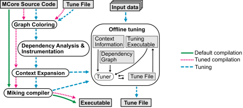
Figure 5. There are three possible flows through the Miking compiler toochain: default compilation (green solid arrows); tuned compilation (dotted magenta-colored arrows); and tuning (dashed blue arrows). Sections 6.2–6.4 give a detailed explanation of each flow. In the figure, artifacts are marked grey and has sharp corners, while transformations are white and rounded.

6.1. The Miking Compiler Toolchain

Miking is a general language system for developing domain-specific and general-purpose languages. The Miking compiler is self-hosting (bootstrapped with OCaml). The core language of the Miking system is called MCore (Miking Core) and is a small functional language. A key language feature of MCore is language fragments. A language fragment defines the abstract syntax and semantics of a fragment of a programming language. By composing several language fragments, new languages are built in a modular way. To extend the Miking compiler toolchain with holes, we create a new language fragment defining the abstract syntax and semantics of holes, and compose this fragment with the main MCore language. The holes are transformed away before the compilation of the program. The motivation for implementing our methodology in Miking is partly because the system is well-designed for implementing language extensions and program transformations, and partly because the methodology can be incorporated in any language developed in Miking.

The Miking toolchain consists of approximately $300$ files and $55,000$ lines of MCore code (out of which approx. $30$$\%$ is either blank lines or comments). The contribution of this paper is the part implementing holes (including language extensions, program transformations, tuning, tuned compilation and dependency analysis). This part consists of $18$ files and approx. $5,000$ lines of code (approx. $30$$\%$ blank lines or comments).

6.2. Default Compilation

The green solid path in Figure 5 shows default compilation. In this path, each hole in the program is statically replaced by its default value. The resulting program is compiled into an executable. Default compilation is useful during development of a program, as tuning can take considerately longer time than default compilation.

6.3. Tuned Compilation

The dotted magenta-colored path in Figure 5 shows tuned compilation. In this scenario, the program and the tune file are given as input to the graph coloring, followed by context expansion (Section 3). The context expansion statically inserts the tuned values for each context into the program. Finally, the program is compiled into an executable. Tuned compilation is done after tuning has been performed, in order to create an executable where the holes are assigned to the tuned values. Optionally, tuned compilation can be performed automatically after tuning.

6.4. Tuning

The blue dashed flow in Figure 5 shows the offline tuning. The program and the tune file (optional) are given as input to the graph coloring. If the tune file is provided, then these values are considered defaults, instead of the values provided via the default keyword. The graph coloring outputs (i) context information about the holes, which is used in the offline tuning, and in later transformation stages, and (ii) a transformed program. Next, the dependency analysis and instrumentation (Section 4) computes a dependency graph, which is also used in the offline tuning, and an instrumented program. The last transformation stage, context expansion, replaces each hole with code that looks up its current calling context. The context expansion sends the context information and the dependency graph to the offline tuning, and the transformed program to the Miking compiler. The Miking compiler creates an executable to be used during tuning, the (tuning executable). The offline tuning takes the context information, dependency graph, tuning executable, and a set of input data as input. The tuner maintains a temporary tune file, which contains the current values of the holes. In each search iteration, the tuning executable reads these values from the file, and the tuner measures the runtime of the program on the set of input data. When the tuning finishes, the tuner writes the best-found values to a final tune file.

The tuner first reduces the search space using the dependency graph and then applies dependency-aware tuning (Section 5). The stopping condition for the tuning is configurable by the user and is either a maximum number of search iterations, or a timeout value.

7. Empirical Evaluation

This section evaluates the implementation. The purpose is to demonstrate that the approach scales to real-world use cases, and to show that context-sensitive holes are useful in these settings. Specifically, we evaluate the following claims:

Claim 1::

We can express implementation choices in real-world and non-trivial programs using context-sensitive holes.

Claim 2::

Dependency analysis reduces the search space of real-world and non-trivial tuning problems.

The evaluation consists of three case studies of varying sizes and from different domains. Two of the case studies, probabilistic programming and Miking compiler, are real-world applications not originally written for the purpose of this evaluation. The third case study, $k$-nearest neighbor classification, is of smaller size, yet is a non-trivial program. The experiments are run under Linux Ubuntu 18.04 ($64$ bits) on an Intel Xeon Gold 6148 of $2.40$ GHz, with $20$ cores, hyperthreading enabled ($2$ threads per core). The computer has $64$ GB RAM and a $1$ MB L2 cache. As backend compiler for the Miking compiler, we use the OCaml compiler available as an OPAM switch 4.12.0+domains. At the time of writing, this is the latest OCaml compiler with multicore support.

7.1. $k$-Nearest Neighbor Classification

This case study consists of a variant of the running example in Section 4, $k$-NN classification. Again, we consider the three implementation choices of the underlying representation of sequence ($h_{\text{seq}}$), parallelization of the map function ($h_{\text{map}}$), and choice of sorting algorithm ($h_{\text{sort}}$). We assume that the performance of these choices depends on the size of the input data, and that we are interested in tuning the classifier for a range of different sizes of the data set. We believe that for small data sets, the sequence representation cons list is more efficient than Rope, the map function is more efficient when run sequentially than in parallel, and that insertion sort is more efficient than merge sort, respectively. However, we do not know the threshold values for these choices. Therefore, we let the three base holes $h_{\text{seq}}$, $h_{\text{map}}$ and $h_{\text{sort}}$ be of type IntRange, representing the unknown threshold values. For instance, assuming the $h_{\text{map}}$ hole is called parThreshold, the following: if lti (length seq)parThreshold then smap f seq else pmap f seq, encodes the choice for the map function.

We assume we are interested in data sets of sizes $10^{3}$–$10^{5}$ points. We set the minimum and maximum values of the holes accordingly to ${\leavevmode\lstinline{{\lst@@@set@language\lst@@@set@numbers\lst@@@set@frame\lst@@@set@rulecolor\lst@@@set@numbers\lst@@@set@language\footnotesize{\@listingGroup{ltx_lst_identifier}{min}}}}}=10^{3}$ and max slightly higher than $10^{5}$, say ${\leavevmode\lstinline{{\lst@@@set@language\lst@@@set@numbers\lst@@@set@frame\lst@@@set@rulecolor\lst@@@set@numbers\lst@@@set@language\footnotesize{\@listingGroup{ltx_lst_identifier}{max}}}}}=101,000$, respectively. That is, the min value corresponds to making the first choice (e.g., sequential map) for all input sizes, while the max value corresponds to making the second choice (e.g., parallel map) for all input sizes.

We generate $6$ random sets of data points with dimension $3$, in sizes in the range of interest: $10^{3},2\cdot 10^{4},4\cdot 10^{4},6\cdot 10^{4},8\cdot 10^{4},10^{5}$. We use a step size of $2\cdot 10^{4}$ when tuning, so that hole values with this interval are considered.

The dependency analysis results are that the search space size is reduced by approx. $83\%$ (from $216$ to $36$ configurations). The best found configuration for the threshold values were $21000$, $1000$, and $101000$ for $h_{\text{map}}$, $h_{\text{sort}}$, and $h_{\text{seq}}$, respectively. That is, all input sizes except the smallest runs map in parallel, all input sizes use merge sort, and all input sizes use cons lists as sequence representation. Table 7.1 presents the execution time results of the tuned program compared to the worst configuration. We see that the tuning gives between $3$–$1500$ speedup of the program.

We note that for this case study, allowing for tail-call optimization in the instrumented program (see Section 4.4) is of utmost importance. The sorting functions are tail recursive, so an instrumented program without tail-call optimizations gives non-representative execution times, or even stack overflow for large enough input sizes. The total time for the tuning is approx. $3.5$ hours, and the static analysis takes less than $100$ ms.

Input size	Execution time	Speedup
1000	0.04	3.28
20000	0.09	323.49
40000	0.15	367.06
60000	0.20	919.16
80000	0.25	1056.70
100000	0.30	1569.68

(a) Tuning results for the $k$-NN classifier. The measurements are done on different data sets than were used during tuning. The ’Input size’ column shows the size of each data set. The ’Execution time’ column shows the execution time in seconds for the tuned program for a given input size. The ’Speedup’ column presents the speedup of the tuned program compared to the worst configuration. The worst configuration for each input size is found by measuring the execution time of the program when setting the threshold so that it is below respectively above the given input size, for each of the three holes. That is, in total there are $8$ ($=2^{3}$) candidate configurations for each input size.

	Sequential	Parallel (worst)
Rope	16.8	1.96
List	18.4	1.94

(b) Speedup of the tuned probabilistic program. The numbers show the speedup of the best found configuration (Rope and parallel map using a chunk size of 610 elements), compared to the other configurations. The ’Rope’ and ’List’ rows are using the respective sequence representation. The ’Sequential’ column uses sequential map, and the ’Parallel (worst)’ column uses parallel map with the chunk size giving the worst execution time. For both Rope and List, the worst choice for the chunk size is $10$ elements. The execution time of each program is measured $10$ times, and the speedup is calculated as the ratio of the mean execution time of the program divided by the mean of the baseline. The execution time of the baseline (the tuned program) is $7.1\pm 0.06$ seconds (mean and standard deviation over $10$ runs).

(c) Results for the $k$-NN and the probabilistic programming case studies.

7.2. Probabilistic Programming

This case study considers a probabilistic programming framework developed consisting of approx. $150$ files and $1,500$ lines of MCore code. Note that the majority of this code is the standard MCore code of the general purpose program and that the probabilistic programming parts consists of a minimal extension. We focus on the inference backend of the framework, using the importance sampling inference method. The inference is a core part of the framework, and is used when solving any probabilistic programming model. We tune the underlying sequence representations and the map function within the inference backend. The sequence representation is either cons list or Rope. The map function chooses between a sequential or parallel implementation. In addition, we tune the chunk size of the parallel implementation (see Example 2.4).

We use a simple probabilistic model representing the outcome of tossing a fair coin. The model makes $10,000$ observations of a coin flip from a Bernoulli distribution, and infers the posterior distribution, given a Beta prior distribution. We expect that the choices the tuner makes are valid for a given model and number of particles used in the inference algorithm, because these two factors are likely to influence the execution time of the map function. Once a given model is tuned, however, it does not need to be re-tuned for other sets of observed data, as long as the number of observations is the same.

We tune the model using $30,000$ particles for the inference algorithm. The tuner chooses to use Rope as sequence representation in combination with parallel map with a chunk size of $610$ elements. Table 6(b) shows the speedup of the best found configuration compared to the others. For instance, we see that we get a speedup of $1.96$ when using a chunk size of $610$ for Rope compared to using the worst chunk size ($10$). The total tuning time for the program is approx. $6$ minutes.

7.3. Miking Compiler

This case study considers the bootstrapping compiler, a subset of the Miking compiler toolchain. The purpose is to test the dependency for a problem of larger scale. For each sequence used within the compiler, we express the choice of which underlying representation to use (Rope or list) using a context-sensitive hole. By default, the compiler uses Rope. Because the main use of sequences within the compiler consists of string manipulation, which is very efficient using Rope, we do not believe there is much to gain from using lists. However, the purpose of this experiment is not to improve the execution time of the compiler, but rather to show search space reduction. After the context expansion, there are in total $2,309$ holes. That is, the size of the original search space is $2^{2309}$. After applying dependency analysis, the search space is reduced to $2^{924}$. By filtering out all measuring points that have a mean execution time of less then $10$ ms, the search space is further reduced to $2^{816}$. The total time of the static analysis is approx. $16$ minutes, which is considerably higher than for the previous case studies, due to the size of this program.

When performing this case study, we choose to disable the feature of the instrumentation that allows for tail-call optimization, because of an identified problem with this feature. We only observe this problem for this large-scale program; for the other case studies the correctness of the instrumentation is validated manually and by assertions within the instrumented code.

7.4. Discussion

This section relates the claims with the results from the case studies, and discusses correctness of possible hole values.

This evaluation considers two claims and three case studies. Claim 1, expressibility of implementation choices in real-world and non-trivial programs, is shown in all three case studies. Using holes, we can encode the automatic selection of algorithms and data structures, as well as parallelization choices. We can also encode dependencies on data size in the program, using threshold values. We address Claim 2 in the $k$-NN classification and Miking compiler case studies. In both these cases, the search spaces are considerably reduced. We observe, especially from the Miking compiler case study, that a possible area for improvement in the dependency analysis is the call graph analysis step (Section 4.3.2). The reason is that for a large program, dependencies from potential executions nested measuring points within branches in match expressions quickly accumulates, giving a quickly growing search space. By taking into account that the execution of the nested points are only conditionally dependent on the condition of the match expressions, we can reduce the search space further.

An essential and challenging aspect when programming in general is the functional correctness of the program. When programming with holes, this aspect can become even more challenging, as combinations of hole values form a (sometimes complicated) set of possible programs. The typical software engineering approach for increasing confidence of correctness is to use testing. As it turns out, testing can also aid us in the case of programming with holes. The MCore language has built-in support for tests (via the language construct utest), and these are stripped away unless we provide the --test flag. By providing the --test flag when invoking the tuning stage, the tuner will run the tests during tuning, using the currently evaluated hole values. The result is a slight degradation in tuning time but no overhead in the final tuned binary. As a practical example, we use utests in the $k$-NN case study in this evaluation in order to ensure that the classifier indeed chooses the correct class for some test data sets.

8. Related Work

This section discusses related work within auto-tuners, by partitioning them into domain-specific and generic tuners. We also discuss work using static analysis within auto tuning.

Many successful auto-tuners target domain-specific problems. SPIRAL (Franchetti et al., 2018) is a tuning framework within the digital signal processing domain, ATLAS (Whaley, 2011) tunes libraries for linear algebra, FFTW (Frigo, 1999) targets fast Fourier transforms, PetaBrikcs (Ansel et al., 2009) focuses on algorithmic choice and composition, and the work by (Li et al., 2004) automatically chooses the best sorting algorithm for a given input list. Moreover, within the area of compiler optimizations, a popular research field is auto-tuning the selection and phase-ordering of compiler optimization passes (Ashouri et al., 2019). On the one hand, a natural drawback with a domain-specific tuner is that it is not applicable outside of its problem scope, while generic tuners (such as our framework) can be applied to a wider range of tuning problems. On the other hand, the main strength of domain-specific tuners is that they can use knowledge about the problem in order to reduce the search space. For instance, SPIRAL applies a dynamic programming approach that incrementally builds solutions from smaller sub-problems, exploiting the recursive structure of transform algorithms. Similarly, PetaBricks also applies dynamic programming as a bottom-up approach for algorithmic composition, and the authors of (Li et al., 2004) include the properties of the lists being sorted (lengths and data distribution) in the tuning. Such domain-dependent approaches are not currently applied in our framework, because the tuner has no deep knowledge about the underlying problem. We are therefore limited to generic search strategies. An interesting research problem is investigating how problem-specific information can be incorporated into our methodology, either from the user, or from compiler analyses, or both. Potentially, such information can speed up the tuning when targeting particular problems, while not limiting the generalizability of our approach.

Among the generic tuners, CLTune (Nugteren and Codreanu, 2017) is designed for tuning the execution time of OpenCL kernels, and supports both offline and online tuning. OpenTuner (Ansel et al., 2014) allows user-defined search-strategies and objective functions (such as execution time, accuracy, or code size). ATF (Rasch and Gorlatch, 2019) also supports user-defined search strategies and objectives and additionally supports pair-wise constraints, such as expressing that the value of a variable must be divisible by another variable. The HyperMapper (Nardi et al., 2019) framework has built-in support for multi-objective optimizations so that trade-off curves of e.g. execution time and accuracy can be explored. Our approach is similar to these approaches as we have a similar programming model: defining unknown variables (holes) with a given set of values. The difference is that we support context-sensitive holes, while previous works perform global tuning.

There are a few previous approaches within the field of program tuning using static analysis to speed up the tuning stage. For instance, to collect metrics from CUDA kernels in order to suggest promising parameter settings to the auto tuner (Lim et al., 2017), or static analysis in combination with empirical experiments for auto tuning tensor transposition (Wei and Mellor-Crummey, 2014). To the best of our knowledge, there is no prior work in using static analysis for analyzing dependency among decision variables. One prior work does exploit dependency to reduce the search space (Schaefer et al., 2009), but their approach relies entirely on user annotations specifying the measuring points, the independent code blocks of the program, permutation regions, and conditional dependencies. By contrast, our approach is completely automatic, where the user can refine the automatic dependency analysis with certain annotations, if needed.

9. Conclusion

In this paper, we propose a methodology for programming with holes that enables developers to postpone design decisions and instead let an automatic tuner find suitable solutions. Specifically, we propose two new concepts: (i) context-sensitive holes, and (ii) dependency-aware tuning using static analysis. The whole approach is implemented in the Miking system and evaluated on non-trivial examples and a larger code base consisting of a bootstrapped compiler. We contend that the proposed methodology may be useful in various software domains, and that the developed framework can be used for further developments of more efficient tuning approaches and heuristics.

- (1)
- Ansel et al. (2009) Jason Ansel, Cy P. Chan, Yee Lok Wong, Marek Olszewski, Qin Zhao, Alan Edelman, and Saman P. Amarasinghe. 2009. PetaBricks: a language and compiler for algorithmic choice. In Proceedings of the 2009 ACM SIGPLAN Conference on Programming Language Design and Implementation, PLDI 2009, Dublin, Ireland, June 15-21, 2009, Michael Hind and Amer Diwan (Eds.). ACM, 38–49. https://doi.org/10.1145/1542476.1542481
- Ansel et al. (2014) Jason Ansel, Shoaib Kamil, Kalyan Veeramachaneni, Jonathan Ragan-Kelley, Jeffrey Bosboom, Una-May O’Reilly, and Saman P. Amarasinghe. 2014. OpenTuner: an extensible framework for program autotuning. In International Conference on Parallel Architectures and Compilation, PACT ’14, Edmonton, AB, Canada, August 24-27, 2014, José Nelson Amaral and Josep Torrellas (Eds.). ACM, 303–316. https://doi.org/10.1145/2628071.2628092
- Ashouri et al. (2019) Amir H. Ashouri, William Killian, John Cavazos, Gianluca Palermo, and Cristina Silvano. 2019. A Survey on Compiler Autotuning using Machine Learning. ACM Comput. Surv. 51, 5 (2019), 96:1–96:42. https://doi.org/10.1145/3197978
- Boehm et al. (1995) Hans-Juergen Boehm, Russell R. Atkinson, and Michael F. Plass. 1995. Ropes: An Alternative to Strings. Softw. Pract. Exp. 25, 12 (1995), 1315–1330. https://doi.org/10.1002/spe.4380251203
- Broman (2019) David Broman. 2019. A Vision of Miking: Interactive Programmatic Modeling, Sound Language Composition, and Self-Learning Compilation. In Proceedings of the 12th ACM SIGPLAN International Conference on Software Language Engineering (SLE ’19). ACM, 55–60.
- Franchetti et al. (2018) Franz Franchetti, Tze Meng Low, Doru-Thom Popovici, Richard Michael Veras, Daniele G. Spampinato, Jeremy R. Johnson, Markus Püschel, James C. Hoe, and José M. F. Moura. 2018. SPIRAL: Extreme Performance Portability. Proc. IEEE 106, 11 (2018), 1935–1968. https://doi.org/10.1109/JPROC.2018.2873289
- Frigo (1999) Matteo Frigo. 1999. A Fast Fourier Transform Compiler. In Proceedings of the 1999 ACM SIGPLAN Conference on Programming Language Design and Implementation (PLDI), Atlanta, Georgia, USA, May 1-4, 1999, Barbara G. Ryder and Benjamin G. Zorn (Eds.). ACM, 169–180. https://doi.org/10.1145/301618.301661
- Gecode Team (2006) Gecode Team. 2006. Gecode: A Generic Constraint Development Environment. Available from http://www.gecode.org/.
- Hoos (2012) Holger H. Hoos. 2012. Programming by optimization. Commun. ACM 55, 2 (2012), 70–80. https://doi.org/10.1145/2076450.2076469
- Li et al. (2004) Xiaoming Li, María Jesús Garzarán, and David A. Padua. 2004. A Dynamically Tuned Sorting Library. In 2nd IEEE / ACM International Symposium on Code Generation and Optimization (CGO 2004), 20-24 March 2004, San Jose, CA, USA. IEEE Computer Society, 111–124. https://doi.org/10.1109/CGO.2004.1281668
- Lim et al. (2017) Robert V. Lim, Boyana Norris, and Allen D. Malony. 2017. Autotuning GPU Kernels via Static and Predictive Analysis. In 46th International Conference on Parallel Processing, ICPP 2017, Bristol, United Kingdom, August 14-17, 2017. IEEE Computer Society, 523–532. https://doi.org/10.1109/ICPP.2017.61
- Nardi et al. (2019) Luigi Nardi, Artur L. F. Souza, David Koeplinger, and Kunle Olukotun. 2019. HyperMapper: a Practical Design Space Exploration Framework. In 27th IEEE International Symposium on Modeling, Analysis, and Simulation of Computer and Telecommunication Systems, MASCOTS 2019, Rennes, France, October 21-25, 2019. IEEE Computer Society, 425–426. https://doi.org/10.1109/MASCOTS.2019.00053
- Nielson et al. (1999) Flemming Nielson, Hanne Riis Nielson, and Chris Hankin. 1999. Principles of program analysis. Springer. https://doi.org/10.1007/978-3-662-03811-6
- Nugteren and Codreanu (2017) Cedric Nugteren and Valeriu Codreanu. 2017. CLTune: A Generic Auto-Tuner for OpenCL Kernels. CoRR abs/1703.06503 (2017). arXiv:1703.06503 http://arxiv.org/abs/1703.06503
- Perron and Furnon (2019) Laurent Perron and Vincent Furnon. 2019. OR-Tools. Google. https://developers.google.com/optimization/
- Rasch and Gorlatch (2019) Ari Rasch and Sergei Gorlatch. 2019. ATF: A generic directive-based auto-tuning framework. Concurr. Comput. Pract. Exp. 31, 5 (2019). https://doi.org/10.1002/cpe.4423
- Rossi et al. (2006) Francesca Rossi, Peter van Beek, and Toby Walsh (Eds.). 2006. Handbook of Constraint Programming. Foundations of Artificial Intelligence, Vol. 2. Elsevier. https://www.sciencedirect.com/science/bookseries/15746526/2
- Schaefer et al. (2009) Christoph A. Schaefer, Victor Pankratius, and Walter F. Tichy. 2009. Atune-IL: An Instrumentation Language for Auto-tuning Parallel Applications. In Euro-Par 2009 Parallel Processing, 15th International Euro-Par Conference, Delft, The Netherlands, August 25-28, 2009. Proceedings (Lecture Notes in Computer Science, Vol. 5704), Henk J. Sips, Dick H. J. Epema, and Hai-Xiang Lin (Eds.). Springer, 9–20. https://doi.org/10.1007/978-3-642-03869-3_5
- Wei and Mellor-Crummey (2014) Lai Wei and John M. Mellor-Crummey. 2014. Autotuning Tensor Transposition. In 2014 IEEE International Parallel & Distributed Processing Symposium Workshops, Phoenix, AZ, USA, May 19-23, 2014. IEEE Computer Society, 342–351. https://doi.org/10.1109/IPDPSW.2014.43
- Whaley (2011) R. Clint Whaley. 2011. Automatically Tuned Linear Algebra Software (ATLAS). In Encyclopedia of Parallel Computing, David A. Padua (Ed.). Springer, 101. https://doi.org/10.1007/978-0-387-09766-4_2061