E-backtesting

Abstract

In the recent Basel Accords, the Expected Shortfall (ES) replaces the Value-at-Risk (VaR) as the standard risk measure for market risk in the banking sector, making it the most important risk measure in financial regulation. One of the most challenging tasks in risk modeling practice is to backtest ES forecasts provided by financial institutions. To design a model-free backtesting procedure for ES, we make use of the recently developed techniques of e-values and e-processes. Model-free e-statistics are introduced to formulate e-processes for risk measure forecasts, and unique forms of model-free e-statistics for VaR and ES are characterized using recent results on identification functions. For a given model-free e-statistic, optimal ways of constructing the e-processes are studied. The proposed method can be naturally applied to many other risk measures and statistical quantities. We conduct extensive simulation studies and data analysis to illustrate the advantages of the model-free backtesting method, and compare it with the ones in the literature.

Keywords: E-values, e-processes, Expected Shortfall, Value-at-Risk, identification function.

1 Introduction

Forecasting risk measures is important for financial institutions to calculate capital reserves for risk management purposes. Regulators are responsible to monitor whether risk forecasts are correctly reported by conducting hypothesis tests known as backtests (see e.g., Christoffersen, 2011; McNeil et al., 2015, for general treatments). Regulatory backtests have several features distinct from traditional testing problems; see Acerbi and Székely (2014) and Nolde and Ziegel (2017). First, risk forecasts and realized losses arrive sequentially over time. Second, due to frequently changing portfolio positions and the complicated temporal nature of financial data, the losses and risk predictions are neither independent nor identically distributed, and they do not follow any standard time-series models. Third, the tester (e.g., a regulator) is concerned about risk measure underestimation, which means high insolvency risk, whereas overestimation (i.e., being conservative) is secondary or acceptable. Fourth, the tester does not necessarily accurately know the underlying model used by a financial institution to produce risk predictions.

In financial practice, a well-adopted simple approach exists for backtesting the Value-at-Risk (VaR), which is the so-called three-zone approach based on binomial tests described in BCBS (2013); this approach is model-free in the sense that one directly tests the risk forecast without testing any specific family of models. The Basel Committee on Banking Supervision (BCBS, 2016) has replaced VaR by the Expected Shortfall (ES) as the standard regulatory measure for market risk, mostly due to the convenient properties of ES, in particular, being able to capture tail risk. However, as discussed by Gneiting (2011), ES is not elicitable, and backtesting ES is substantially more challenging than VaR. Table 1 summarizes the main features of existing methods backtesting ES. To the best of our knowledge, there is no model-free non-asymptotic backtesting method for ES. Moreover, except for Hoga and Demetrescu (2022), most of the backtesting methods in the existing literature only work for a fixed data size, and are thus not valid under option stopping, or equivalently, not anytime valid (see e.g., Chu et al., 1996, for discussions). This creates limitations to financial regulation practice where early rejections are highly desirable.

Literature	Parametric or dependence assumptions	Forecast structural assumptions	Fixed sample size	Asymptotic test	Reliance on VaR or distributional forecasts
MF00	yes	yes	yes	yes	yes
AS14	yes	yes	yes	yes	yes
DE17	yes	yes	yes	yes	yes
NZ17	yes	yes	yes	yes	yes
BD22	yes	yes	yes	yes	no
HD22	yes	yes	no	no	yes
This paper	no	no	no	no	yes

Table 1: Comparison of existing backtesting methods for ES

Notes: We use shortcuts MF00 for McNeil and Frey (2000), AS14 for Acerbi and Székely (2014), DE17 for Du and Escanciano (2017), NZ17 for Nolde and Ziegel (2017), BD22 for Bayer and Dimitriadis (2022), and HD22 for Hoga and Demetrescu (2022). Parametric or dependence assumptions refer to those on loss distributions, time series models, stationarity, or strong mixing. Forecast structural assumptions refer to requirements on the forms and properties of risk forecasts. Acerbi and Székely (2014) proposed three methods of backtesting ES; The first two methods do not require specific forms of ES forecasts, but the third method requires ES to be estimated as realized ranks.

In this paper, we develop a model-free backtesting method for risk measures, including ES, using the concepts of e-values and e-tests (Shafer, 2021; Vovk and Wang, 2021; Grünwald et al., 2020). E-tests have important advantages over classical statistical tests (p-tests) based on p-values. (Wang and Ramdas, 2022, Section 2) collect many reasons for using e-values and e-tests, regarding high-dimensional asymptotics, composite models, sequential (any-time valid) inference, information accumulation, and robustness to model misspecification and dependence; other advantages of e-values have been illustrated by Grünwald et al. (2020), Vovk and Wang (2021) and Vovk et al. (2022). As a particularly relevant feature to our context, our proposed e-tests allow regulators to get alerted early as the e-process accumulates to a reasonably large value. This is different from scientific discoveries (such as genome studies) where a scientist may not be entitled to reject a hypothesis based on merely “substantial” evidence. Noticing this, a multi-zone approach similar to the three-zone approach can be developed by setting different e-value thresholds in financial regulation.

The main contribution of this paper is four-fold: First, we introduce the new notion of model-free e-statistics and propose e-backtesting methods. In particular, we obtain model-free e-statistics for ES in Section 2 (Theorem 1), allowing us to construct e-processes to backtest ES, as well as other risk measures in Section 3 (Theorem 2). The backtesting method for VaR and ES is discussed in Section 4. Second, with model-free e-statistics chosen, the next important step to construct an e-process is by choosing a suitable betting process, which we address in Section 5. We propose three methods to calculate the betting processes based on data. It turns out that these methods are asymptotically optimal (equivalent to an oracle betting process) under different situations (Theorem 3). Third, we characterize model-free e-statistics for the mean, the variance, VaR (Theorem 4), and ES (Theorem 5) in Section 6 by establishing a link between model-free e-statistics and identification functions. All model-free e-statistics for these functionals take similar forms as mixtures between $1$ and a simple model-free e-statistic. Finally, through the simulation study and data analysis in Sections 7 and 8, we demonstrate detailed procedures of backtesting VaR and ES using e-values for practical operations of financial regulations. In addition to our main content, Appendix A shows the betting processes calculated via Taylor approximation for VaR and ES; Appendix B discusses the link between model-free e-statistics and identification functions in preparation for the characterization results in Section 6; except for Theorems 1 and Theorem 3, proofs of all results are relegated to Appendix C; Appendix D contains some necessary details of our simulation and data analysis. To support our new methodology, extended simulation studies and data analyses are presented in the separate paper Wang et al. (2022) for the interested reader.

1.1 Related literature

Besides financial regulation, evaluating forecasting models and methods for major economic variables is also essential in the decision-making processes of government institutions and regulatory authorities. Earlier work on predictive ability tests and forecast selection includes Diebold and Mariano (1995), whose method was extended by West (1996), Clark and McCracken (2001), and Giacomini and White (2006). Unconditional backtests of VaR were considered by Kupiec (1995) on testing Bernoulli distributions, which were extended by Christoffersen (1998) to include testing independence of the $\mathrm{VaR}$-violations. Engle and Manganelli (2004) tested conditional autoregressive VaR; Berkowitz et al. (2011) unified existing evaluation methods of VaR; and Ziggel et al. (2014) proposed a Monte Carlo simulation-based backtesting method for VaR.

Due to its increasing importance and challenging nature, there are ample studies in the more recent literature on backtesting ES with different approaches and limitations. McNeil and Frey (2000) proposed bootstrap tests with iid innovations; Acerbi and Székely (2014, 2017) studied three backtesting methods under independent losses; Du and Escanciano (2017) designed parametric test using cumulative violations; Nolde and Ziegel (2017) studied comparative backtests among forecasting methods; Bayer and Dimitriadis (2022) built backtesting through a linear regression model; and Hoga and Demetrescu (2022) proposed sequential monitoring based on parametric distributions. The main features of all approaches are summarized in Table 1.

The literature on e-values has also been growing fast recently. E-values were used in the early literature in different disguises, although the term “e-value” was proposed by Vovk and Wang (2021). For instance, e-values and e-tests were essentially used in the work of Wald (1945) and Darling and Robbins (1967), and they are central to the ideas of testing by betting and martingales (Shafer et al., 2011; Shafer and Vovk, 2019) and universal inference (Wasserman et al., 2020). E-values are shown to be useful in multiple hypothesis testing with dependence (Vovk and Wang, 2021), parametric tests with optional sampling (Grünwald et al., 2020), false discovery rate control (Wang and Ramdas, 2022), and many other statistical applications. We refer to the recent survey paper of Ramdas et al. (2022) for an overview.

2 E-values and model-free e-statistics

2.1 Definition and examples

Let $(\Omega,\mathcal{F},\mathbb{P})$ be any probability space, and $\mathfrak{P}$ be the set of probability measures on $(\Omega,\mathcal{F})$. A (composite) hypothesis $H$ is a subset of $\mathfrak{P}$. A hypothesis $H$ is simple if it is a singleton. Following the terminology of Vovk and Wang (2021), an e-variable for $H\subseteq\mathfrak{P}$ is an extended random variable $E:\Omega\to[0,\infty]$ such that $\mathbb{E}^{P}[E]\leqslant 1$ for each $P\in H$. We denote by $\mathcal{E}_{H}$ the set of e-variables for a hypothesis $H$ and by $\mathcal{E}_{P}$ the set of e-variables for the simple hypothesis $\{P\}$. An e-test rejects the hypothesis $H$ if a realized e-variable, called an e-value, is larger than a threshold. A common rule of thumb is that an e-value of $10$ represents strong evidence. A non-negative stochastic process $(E_{t})_{t\in K}$, $K\subseteq\mathbb{N}$, adapted to a given filtration, is an e-process for $H$ if $\mathbb{E}^{P}[E_{\tau}]\leqslant 1$ for all stopping times $\tau$ taking values in $K$ and each $P\in{H}$.

Let $d$ be a positive integer. The model space $\mathcal{M}$ is a set of distributions on $\mathbb{R}$. The value of the functional $\psi=(\rho,\phi_{1},\dots,\phi_{d-1}):\mathcal{M}\to\mathbb{R}^{d}$ represents the collection of available statistical information, where $\rho$ is the risk prediction to be tested, and $\phi$ contains auxiliary information. If $d=1$, then the only available information is the predicted value of $\rho$. Let $\mathcal{M}_{q}$, $\mathcal{M}_{\infty}$, and $\mathcal{M}_{0}$ represent the set of distributions on $\mathbb{R}$ with finite $q$-th moment for $q\in(0,\infty)$, that of compactly supported distributions on $\mathbb{R}$, and that of all distributions on $\mathbb{R}$, respectively. Let $L^{0}$ be a set of random variables on $(\Omega,\mathcal{F},\mathbb{P})$. Define $\psi$ for a random variable $X\in L^{0}$ via $\psi(X)=\psi(F)$, where $F$ is the distribution of $X$. For level $p\in(0,1)$, the Value-at-Risk (VaR) is defined as the lower $p$-quantile:

$$\mathrm{VaR}_{p}(F)=Q_{p}(F)=\inf\{x\in\mathbb{R}:F(x)\geqslant p\},\leavevmode\nobreak\ \leavevmode\nobreak\ F\in\mathcal{M}_{0},$$

and the Expected Shortfall (ES) is defined as

$$\mathrm{ES}_{p}(F)=\frac{1}{1-p}\int_{p}^{1}\mathrm{VaR}_{\alpha}(F)\,\mathrm{d}\alpha,\leavevmode\nobreak\ \leavevmode\nobreak\ F\in\mathcal{M}_{1}.$$

VaR and ES belong to the class of dual utilities in Yaari (1987) and Schmeidler (1989). For $\psi=(\rho,\phi_{1},\dots,\phi_{d-1})$, the natural domains of $\rho,\phi_{1},\dots,\phi_{d-1}$ are not necessarily identical, and the domain of $\psi$ is set to be their intersection. In the following Definitions 1 and 2, we introduce the key tool we use for our e-tests.

Definition 1 (Model-free e-statistics).

Let $\mathcal{P}\subseteq\mathcal{M}$. An $\mathcal{P}$-model-free e-statistic for $\psi:\mathcal{M}\to\mathbb{R}^{d}$ is a measurable function $e:\mathbb{R}^{d+1}\to[0,\infty]$ satisfying $\int_{\mathbb{R}}e(x,\psi(F))\,\mathrm{d}F(x)\leqslant 1$ for each $F\in\mathcal{P}$. If $\mathcal{P}=\mathcal{M}$, then we simply call $e$ a model-free e-statistic for $\psi$.

To consider $\mathcal{P}$-model-free e-statistics for $\psi$ in Definition 1, it suffices to consider the restriction of $\psi$ on $\mathcal{P}$. Using the language of e-variables, a model-free e-statistic for $\psi$ is a function $e$ such that $e(X,\psi(F))\in\mathcal{E}_{\mathbb{P}}$ for each $F\in\mathcal{P}$, where $X$ has distribution $F$ under $\mathbb{P}$. The term “model-free” reflects that the e-statistic is valid for all $F\in\mathcal{P}$.

Definition 2 (Model-free e-statistics testing $\rho$).

Let $\mathcal{P}\subseteq\mathcal{M}$. For $\psi=(\rho,\phi):\mathcal{M}\to\mathbb{R}\times\mathbb{R}^{d-1}$, a $\mathcal{P}$-model-free e-statistic $e:\mathbb{R}^{d+1}\to[0,\infty]$ for $\psi=(\rho,\phi)$ is testing $\rho$ if $\int_{\mathbb{R}}e(x,r,z)\,\mathrm{d}F(x)>1$ for all $(r,z)\in\psi(\mathcal{P})$ and $F\in\mathcal{P}$ with $\rho(F)>r$. The e-statistic is strictly testing $\rho$ if $(x,r,z)\mapsto e(x,r,z)$ is decreasing in $r$. If $d=1$, $e$ is simply called a $\mathcal{P}$-model-free e-statistic testing $\rho$.

Intuitively, Definition 1 addresses the validity of the e-test: if a true value of the risk prediction for $\psi=(\rho,\phi)$ is provided, then the e-statistic will have a mean that is no larger than $1$. On the other hand, Definition 2 addresses the consistency of the e-test: if the risk $\rho$ is underestimated, then the e-statistic will have a mean that is larger than $1$, regardless of whether the prediction of the auxiliary functional $\phi$ is truthful. The special case where $d=1$, i.e., no auxiliary functional $\phi$ is involved, will be discussed in detail in Section 6.1.

We are only interested in forecast values $(r,z)$ in the set $\psi(\mathcal{P})$. Any forecast values outside $\psi(\mathcal{P})$ can be rejected directly.

Our idea of model-free e-statistics specifically addresses the underestimation of $\rho$, which is consistent with the motivation in regulatory backtesting. If an e-statistic is strictly testing a risk measure $\rho$, then an overestimation of the risk is rewarded: An institution being scrutinized by the regulator can deliberately report a higher risk value (which typically means higher capital reserve) to pass to the regulatory test, thus rewarding prudence.

First, we give a few examples of model-free e-statistics for some common risk measures. Throughout, we use the convention that $0/0=1$ and $1/0=\infty$, and let $\mathbb{R}_{+}=[0,\infty)$.

Example 1 (Model-free e-statistic testing the mean).

Let $\mathcal{P}$ be the set of distributions on $\mathbb{R}_{+}$ in $\mathcal{M}_{1}$. Define the function $e(x,r)=x/r$ for $x,r\geqslant 0$. In this case, we have $\mathbb{E}[e(X,\mathbb{E}[X])]=1$ for all random variables $X$ with distribution in $\mathcal{P}$. Moreover, for any such $X$, $\mathbb{E}[X]>r\geqslant 0$ implies $\mathbb{E}[e(X,r)]>1$. Therefore, $e$ is a $\mathcal{P}$-model-free e-statistic strictly testing the mean.

Example 2 (Model-free e-statistic for $(\mathrm{var},\mathbb{E})$ testing the variance).

Consider $(\mathrm{var},\mathbb{E}):\mathcal{M}_{2}\to\mathbb{R}^{2}$. For all random variables $X$ with distribution in $\mathcal{M}_{2}$, we have

$$\mathbb{E}[e(X,\mathrm{var}(X),\mathbb{E}[X])]=\frac{\mathbb{E}[(X-\mathbb{E}[X])^{2}]}{\mathrm{var}(X)}=1.$$

Moreover, since $z=\mathbb{E}[X]$ minimizes $\mathbb{E}[(X-z)^{2}]$ over $z\in\mathbb{R}$ and $\mathrm{var}(X)=\mathbb{E}[(X-\mathbb{E}[X])^{2}]$, $\mathrm{var}(X)>r\geqslant 0$ implies

$$\mathbb{E}[e(X,r,z)]=\frac{\mathbb{E}[(X-z)^{2}]}{r}\geqslant\frac{\mathrm{var}(X)}{r}>1.$$

Hence, $e(x,r,z)=(x-z)^{2}/r$ for $x,z\in\mathbb{R}$ and $r\geqslant 0$ is a model-free e-statistic for $(\mathrm{var},\mathbb{E})$ strictly testing the variance.

Example 3 (Model-free e-statistic testing a quantile).

Take $p\in(0,1)$. Define the function

$$e_{p}^{Q}(x,r)=\frac{1}{1-p}\mathds{1}_{\{x>r\}},\leavevmode\nobreak\ \leavevmode\nobreak\ x,r\in\mathbb{R}.$$ (1)

We have $\mathbb{E}[e(X,Q_{p}(F))]\leqslant 1$ for any random variable $X$ with distribution $F$. Moreover, $Q_{p}(F)>r$ implies $\mathbb{P}(X>r)>1-p$, and hence $\mathbb{E}[e(X,r)]>1$. Therefore, $e$ is a model-free e-statistic strictly testing the $p$-quantile.

Example 4 (Model-free e-statistic testing an expected loss).

For some $a\in\mathbb{R}$, let $\ell:\mathbb{R}\to[a,\infty)$ be a function that is interpreted as a loss. Define the function $e(x,r)=(\ell(x)-a)/{(r-a)}$ for $x\in\mathbb{R}$ and $r\geqslant a$. Analogously to Example 1, $e$ is a model-free e-statistic strictly testing the expected loss $F\mapsto\int\ell\,\mathrm{d}F$ on its natural domain.

The choice of a model-free e-statistic $e$ for $\psi$ is not necessarily unique. For instance, a linear combination of $e$ with $1$ with the weight between $0$ and $1$ is also a model-free e-statistic for $\psi$. Depending on the specific situation, either e-statistic may be useful in practice.

Remark 1.

The functional $\psi=(\rho,\phi)=(\mathrm{var},\mathbb{E})$ in Example 2 is an example of a Bayes pair, that is, a there exists a measurable function $L:\mathbb{R}^{d+1}\to\mathbb{R}$, called the loss function, such that

$$\phi(F)\in\operatorname*{arg\,min}_{z\in\mathbb{R}^{d}}\int L(z,x)\,\mathrm{d}F(x)\text{ and }\rho(F)=\min_{z\in\mathbb{R}^{d}}\int L(z,x)\,\mathrm{d}F(x),\quad F\in\mathcal{M},$$ (2)

where $\int L(z,x)\,\mathrm{d}F(x)$ is assumed to be well-defined for each $z\in\mathbb{R}^{d}$, $F\in\mathcal{M}$ (Fissler and Ziegel, 2016; Frongillo and Kash, 2021; Embrechts et al., 2021). Bayes pairs often admit model-free e-statistics. A typical example commonly used in risk management practice is $(\mathrm{ES},\mathrm{VaR})$, which we mainly focus on in this paper.

Next, we see that, for $p\in(0,1)$ the function

$$e^{\mathrm{ES}}_{p}(x,r,z)=\frac{(x-z)_{+}}{(1-p)(r-z)},\leavevmode\nobreak\ \leavevmode\nobreak\ \leavevmode\nobreak\ x\in\mathbb{R},\leavevmode\nobreak\ z\leqslant r.$$ (3)

defines a model-free e-statistic for $(\mathrm{ES}_{p},\mathrm{VaR}_{p})$ testing $\mathrm{ES}_{p}$. Recall the convention that $0/0=1$ and $1/0=\infty$, and set $e^{\mathrm{ES}}_{p}(x,r,z)=\infty$ if $r<z$, which is a case of no relevance since $\mathrm{ES}_{p}(F)\geqslant\mathrm{VaR}_{p}(F)$ for any $F\in\mathcal{M}_{1}$.

Theorem 1.

The function $e^{\mathrm{ES}}_{p}$ is a model-free e-statistic for $(\mathrm{ES}_{p},\mathrm{VaR}_{p})$ strictly testing $\mathrm{ES}_{p}$.

Proof.

By the VaR-ES relation of Rockafellar and Uryasev (2002), for any random variable $X$ with finite mean,

$$\mathrm{VaR}_{p}(X)\in\operatorname*{arg\,min}_{z\in\mathbb{R}}\left\{z+\frac{1}{1-p}\mathbb{E}[(X-z)_{+}]\right\},$$ (4)

and

$$\mathrm{ES}_{p}(X)=\min_{z\in\mathbb{R}}\left\{z+\frac{1}{1-p}\mathbb{E}[(X-z)_{+}]\right\}.$$ (5)

This indicates that $(\mathrm{ES}_{p},\mathrm{VaR}_{p})$ is a Bayes pair by (2) with loss function $L:(z,x)\mapsto z+(x-z)_{+}/(1-p)$. Since $L(z,x)\geqslant z$, for $r\geqslant z$, we have that $e^{\mathrm{ES}}_{p}(x,r,z)=(L(z,x)-z)/(r-z)\geqslant 0$, and it is decreasing in $r$. Furthermore, for $z<r\leqslant\mathrm{ES}_{p}(X)$,

$$\mathbb{E}\left[\frac{L(z,X)-z}{r-z}\right]\geqslant\frac{\mathrm{ES}_{p}(X)-z}{r-z}\geqslant 1$$

with equality if and only if $r=\mathrm{ES}_{p}(X)$. ∎

While Examples 1-4 and Theorem 1 show that interesting model-free e-statistics exist, much more can be said about their general structure; see Section 6.

3 E-backtesting risk measures with model-free e-statistics

We next present a general methodology for backtesting risk measures via model-free e-statistics in a sequential setting.

Let $T$ be any time horizon, which may be fixed, infinite, or adaptive, i.e., depending on the data observed. The flexibility of infinite or data-dependent time horizons is a feature of e-tests, which allows us to address situations more general than the ones considered in the literature, e.g., Hoga and Demetrescu (2022), where $T$ is a pre-specified fixed time horizon and the tester has to start over when time $T$ is reached. For any positive integer $n$, denote by $[n]=\{1,\dots,n\}$, and for $n=\infty$ it is $[n]=\mathbb{N}$, the set of positive integers.

Let the $\sigma$-algebra $\mathcal{F}_{t}$ represent all the available information up to time $t\in[T]$, such that $\mathcal{F}_{m}\subseteq\mathcal{F}_{n}$ for all $m\leqslant n$. Let $(L_{t})_{t\in[T]}$ be a sequence of realized losses that are adapted to the filtration $(\mathcal{F}_{t})_{t\in[T]}$. Denote by $\rho(L_{t}|\mathcal{F}_{t-1})$ and $\phi(L_{t}|\mathcal{F}_{t-1})$, respectively, the values of $\rho$ and $\phi$ applied to the conditional distribution of $L_{t}$ given $\mathcal{F}_{t-1}$. Let $r_{t}$ and $z_{t}$ be forecasts for $\rho(L_{t}|\mathcal{F}_{t-1})$ and $\phi(L_{t}|\mathcal{F}_{t-1})$ made at time $t-1$, respectively. Note that $\rho(L_{t}|\mathcal{F}_{t-1})$ and $\phi(L_{t}|\mathcal{F}_{t-1})$ are themselves random variables and $\mathcal{F}_{t-1}$-measurable for all relevant functionals of interest (see e.g., Fissler and Holzmann, 2022).

We assume that the risk forecasts $r_{t}$ and $z_{t}$ are obtained based on past market information and all other possible factors that may affect the decisions of risk predictors in financial institutions. For instance, the information may even include throwing a die or random events such as coffee spilling; all these events up to time $t-1$ are included in $\mathcal{F}_{t-1}$.

We test the following null hypothesis:

$$H_{0}:\leavevmode\nobreak\ \leavevmode\nobreak\ r_{t}\geqslant\rho(L_{t}|\mathcal{F}_{t-1})\leavevmode\nobreak\ \mbox{and}\leavevmode\nobreak\ z_{t}=\phi(L_{t}|\mathcal{F}_{t-1})\leavevmode\nobreak\ \leavevmode\nobreak\ \mbox{ for $t\in[T]$}.$$ (6)

Rejecting (6) implies, in particular, rejecting $r_{t}=\rho(L_{t}|\mathcal{F}_{t-1})$ and $z_{t}=\phi(L_{t}|\mathcal{F}_{t-1})$ for all $t\in[T]$. In the special case that $d=1$ (i.e. we do not need auxiliary information from $\phi$), (6) becomes

$$H_{0}:\leavevmode\nobreak\ \leavevmode\nobreak\ r_{t}\geqslant\rho(L_{t}|\mathcal{F}_{t-1})\leavevmode\nobreak\ \leavevmode\nobreak\ \mbox{ for $t\in[T]$}.$$

Remark 2.

Since $\rho$ is the regulatory risk measure of interest, over-predicting $\rho$ is conservative. On the other hand, $\phi$ represents some additional statistical information and it may not relate to measuring financial risk. Hence, over-predicting $\phi$ is not necessarily conservative. See Example 5 below for a sanity check. Therefore, it is more natural to test an equality of the auxiliary information $z_{t}$ in (6) instead of an inequality; note also that this hypothesis is still more lenient than testing a specified loss distribution. For the case where a financial institution is conservative for both the risk measures $\rho$ and $\phi$, see Section 4.

For a nonnegative function $e:\mathbb{R}^{d+1}\to[0,\infty]$, let $X_{t}=e(L_{t},r_{t},z_{t})$ for each t. We construct the following stochastic process: $M_{0}=1$ and

$$M_{t}(\bm{\lambda})=(1-\lambda_{t}+\lambda_{t}X_{t})M_{t-1}(\bm{\lambda})=\prod_{s=1}^{t}(1-\lambda_{s}+\lambda_{s}X_{s}),\leavevmode\nobreak\ \leavevmode\nobreak\ t\in[T],$$ (7)

where the process $\bm{\lambda}=(\lambda_{t})_{t\in[T]}$ is chosen such that $\lambda_{t}$ is a function of $(L_{s-1},r_{s},z_{s})_{s\in[t]}$ and takes values in $[0,1]$ for $t\in[T]$. Suppose that $e$ is a model-free e-statistic for $(\rho,\phi):\mathcal{M}\to\mathbb{R}\times\mathbb{R}^{d-1}$. We have by definition that $X_{t}$ is an e-variable conditional on $\mathcal{F}_{t-1}$ under $H_{0}$ for all $t\in[T]$. As suggested by Vovk and Wang (2020), the only admissible (or unwasteful) way to combine these e-variables is through the martingale function (7). The e-process in (7) may be interpreted as the payoffs of a betting strategy against the null hypothesis $H_{0}$ as in Shafer and Vovk (2019). In this betting game, the initial capital is $M_{0}=1$ and all the money is invested at each step. The payoff per capital at each step is $1-\lambda_{t}+\lambda_{t}X_{t}$ for $t\in[T]$. As a result, the player earns money at step $t$ if $X_{t}>1$. In this sense, we call the process $\bm{\lambda}$ in (7) a betting process. The following theorem follows from Ville’s well-known inequality (Ville, 1939), indicating that $(M_{t}(\bm{\lambda}))_{t\in\{0,\dots,T\}}$ in (7) is a non-negative supermartingale, so in particular an e-process under the null hypothesis in (6).

Theorem 2.

Suppose that $e$ is a model-free e-statistic for $(\rho,\phi):\mathcal{M}\to\mathbb{R}\times\mathbb{R}^{d-1}$. Under $H_{0}$ in (6), $(M_{t}(\bm{\lambda}))_{t\in\{0,\dots,T\}}$ in (7) is a non-negative supermartingale with $M_{0}=1$, and for each $\alpha\in(0,1)$,

$$\mathbb{P}\left(\sup_{t\in\{0,\dots,T\}}M_{s}(\bm{\lambda})\geqslant\frac{1}{\alpha}\right)\leqslant\alpha.$$

Based on Theorem 2, we will use the e-test that arises by using the e-variable $M_{\tau}(\bm{\lambda})$ where $M(\bm{\lambda})$ is given by (7) and $\tau$ is the stopping time $\min\{T,\inf\{t\geqslant 0:M_{t}(\bm{\lambda})\geqslant 1/\alpha\}\}$. This is common practice in testing with e-values.

Remark 3.

Our framework of backtesting risk measures can be applied to a simpler hypothesis testing problem in a static setting. Suppose that $r$ and $z$ are fixed forecasts of risk measures $\rho:\mathcal{M}\to\mathbb{R}$ and $\phi:\mathcal{M}\to\mathbb{R}^{d}$, respectively, for some random variable $L$. Consider the following testing problem:

$$H_{0}:r\geqslant\rho(L)\leavevmode\nobreak\ \leavevmode\nobreak\ \mbox{and}\leavevmode\nobreak\ \leavevmode\nobreak\ z=\phi(L)\leavevmode\nobreak\ \leavevmode\nobreak\ \mbox{or}\leavevmode\nobreak\ \leavevmode\nobreak\ \widetilde{H}_{0}:(r,z)=(\rho(L),\phi(L)).$$ (8)

We observe iid samples $L_{1},\dots,L_{n}$ from $L$ and assume that the observations arrive sequentially. Suppose that there exists a model-free e-statistic $e:\mathbb{R}^{d+1}\to[0,\infty]$ for $(\rho,\phi)$ testing $\rho$. We obtain e-values under the null hypotheses $H_{0}$ and $\widetilde{H}_{0}$ in (8) given by $e(L_{i},r,z)$, $i\in[n]$. A simulation study on this setting is provided in the separate paper Wang et al. (2022).

4 E-backtesting Value-at-Risk and Expected Shortfall

To put our general ideas in the context of financial regulation, we focus on backtesting VaR and ES in this section. Let $L_{t}$ be the random loss at time $t$. For the case of backtesting VaR, $(r_{t})_{t\in[T]}$ are the forecasts for $\mathrm{VaR}_{p}(L_{t}|\mathcal{F}_{t-1})$, $p\in(0,1)$. As we see in Example 3, the function $e^{Q}_{p}(L_{t},r_{t})$ defined in (1) is an e-variable under the following null hypothesis that we are testing,

$$H_{0}:\leavevmode\nobreak\ \leavevmode\nobreak\ \mbox{$r_{t}\geqslant\mathrm{VaR}_{p}(L_{t}|\mathcal{F}_{t-1})$},\leavevmode\nobreak\ \leavevmode\nobreak\ \leavevmode\nobreak\ \leavevmode\nobreak\ t\in[T].$$

For the case of backtesting ES, $(r_{t})_{t\in[T]}$ are the forecasts for $\mathrm{ES}_{p}(L_{t}|\mathcal{F}_{t-1})$ and $(z_{t})_{t\in[T]}$ are the forecasts for $\mathrm{VaR}_{p}(L_{t}|\mathcal{F}_{t-1})$, $p\in(0,1)$. By Theorem 1, $e^{\mathrm{ES}}_{p}(L_{t},r_{t},z_{t})$ is an e-variable under the following null hypothesis:

$$H_{0}:\leavevmode\nobreak\ \leavevmode\nobreak\ \mbox{$r_{t}\geqslant\mathrm{ES}_{p}(L_{t}|\mathcal{F}_{t-1})$ and $z_{t}=\mathrm{VaR}_{p}(L_{t}|\mathcal{F}_{t-1})$},\leavevmode\nobreak\ \leavevmode\nobreak\ \leavevmode\nobreak\ \leavevmode\nobreak\ t\in[T].$$ (9)

In practice, a financial institution may use a conservative model for risk management purposes, which leads to underestimation of both VaR and ES. In the following proposition, we illustrate that $e^{\mathrm{ES}}_{p}(L_{t},r_{t},z_{t})$ is a valid e-variable in case both $\mathrm{VaR}_{p}(L_{t}|\mathcal{F}_{t-1})$ and $\mathrm{ES}_{p}(L_{t}|\mathcal{F}_{t-1})$ are over-predicted, together with their difference.

Proposition 1.

For $p\in(0,1)$, $(e^{\mathrm{ES}}_{p}(L_{t},r_{t},z_{t}))_{t\in[T]}$ are e-variables for

$$H_{0}:\leavevmode\nobreak\ z_{t}\geqslant\mathrm{VaR}_{p}(L_{t}|\mathcal{F}_{t-1})\leavevmode\nobreak\ \leavevmode\nobreak\ \mbox{and}\leavevmode\nobreak\ \leavevmode\nobreak\ r_{t}-z_{t}\geqslant\mathrm{ES}_{p}(L_{t}|\mathcal{F}_{t-1})-\mathrm{VaR}_{p}(L_{t}|\mathcal{F}_{t-1}),\leavevmode\nobreak\ t\in[T].$$ (10)

The hypothesis $H_{0}$ in (10) is stronger than

$$H_{0}:z_{t}\geqslant\mathrm{VaR}_{p}(L_{t}|\mathcal{F}_{t-1})\leavevmode\nobreak\ \leavevmode\nobreak\ \mbox{and}\leavevmode\nobreak\ \leavevmode\nobreak\ r_{t}\geqslant\mathrm{ES}_{p}(L_{t}|\mathcal{F}_{t-1}).$$ (11)

In contrast to (10), we note that $e^{\mathrm{ES}}_{p}(L_{t},r_{t},z_{t})$ is not necessarily an e-variable for (11). For instance, $\mathbb{E}[e^{\mathrm{ES}}_{p}(L_{t},r_{t},z_{t})]=\infty$ if $r_{t}=z_{t}=\mathrm{ES}_{p}(L_{t}|\mathcal{F}_{t-1})$ and $\mathbb{P}(L_{t}>z_{t})>0$. It implies that over-predicting $\mathrm{VaR}_{p}(L_{t}|\mathcal{F}_{t-1})$ does not always leads to a smaller e-value realized by $e^{\mathrm{ES}}_{p}(L_{t},r_{t},z_{t})$; in contrast, over-predicting $\mathrm{ES}_{p}(L_{t}|\mathcal{F}_{t-1})$ always reduces the resulting e-value. The following example illustrates that a poor VaR forecast could result in large e-values although it is obtained by over-prediction.

Example 5.

For $p\in(0,1)$, a continuously distributed random variable $X$ with $a=\mathrm{VaR}_{p}(X)<\mathrm{ES}_{p}(X)=1$ (this implies $\mathbb{P}(X\leqslant 1)<1$) has a heavier tail than $Y$ with $\mathrm{VaR}_{p}(Y)=\mathrm{ES}_{p}(Y)=1$ (this implies $\mathbb{P}(Y\leqslant 1)=1$). Thus, intuitively, a forecaster producing the random loss $X$ is more conservative than that producing $Y$. This shows that over-predicting both $\mathrm{VaR}_{p}$ and $\mathrm{ES}_{p}$ does not always mean that the forecaster is more conservative about the risk. Our model-free e-statistic $e^{\mathrm{ES}}_{p}$ can detect this, because $\mathbb{E}[e^{\mathrm{ES}}_{p}(X,1,a)]\leqslant 1$ while $\mathbb{E}[e^{\mathrm{ES}}_{p}(X,1,1)]=\infty$, thus correctly rejecting the forecast $(1,1)$ of $(\mathrm{ES}_{p}(X),\mathrm{VaR}_{p}(X))$ but not rejecting the truthful forecast $(1,a)$, although $a<1.$

The following example collects some practical situations of conservative forecasts. In each case, $e^{\mathrm{ES}}_{p}(L_{t},r_{t},z_{t})$ yields a valid e-variable.

Example 6.

1. $r_{t}=\mathrm{ES}_{q}(L_{t}|\mathcal{F}_{t-1})$ and $z_{t}=\mathrm{VaR}_{q}(L_{t}|\mathcal{F}_{t-1})$ for $q>p$:

   $$\mathbb{E}[e^{\mathrm{ES}}_{p}(L_{t},r_{t},z_{t})]=\frac{1-q}{1-p}\mathbb{E}[e^{\mathrm{ES}}_{q}(L_{t},\mathrm{ES}_{q}(L_{t}|\mathcal{F}_{t-1}),\mathrm{VaR}_{q}(L_{t}|\mathcal{F}_{t-1}))]=\frac{1-q}{1-p}<1.$$

   In this situation, $\mathrm{VaR}_{p}$ and $\mathrm{ES}_{p}$ are over-predicted by lifting the confidence level $p$ to $q$. For instance, this may represent the output of a stress-testing scenario which amplifies the probability of extreme losses.

2. $r_{t}=c_{1}\mathrm{ES}_{p}(L_{t}|\mathcal{F}_{t-1})$ and $z_{t}=c_{2}\mathrm{VaR}_{p}(L_{t}|\mathcal{F}_{t-1})\geqslant 0$ for $c_{1}\geqslant c_{2}\geqslant 1$, as justified by Proposition 1. In particular, $\mathrm{VaR}_{p}$ and $\mathrm{ES}_{p}$ can be over-predicted by the same multiplicative factor.

3. $r_{t}=\mathrm{ES}_{p}(L_{t}|\mathcal{F}_{t-1})+b_{1}$ and $z_{t}=\mathrm{VaR}_{p}(L_{t}|\mathcal{F}_{t-1})+b_{2}$ for $b_{1}\geqslant b_{2}\geqslant 0$, as justified by Proposition 1. In particular, $\mathrm{VaR}_{p}$ and $\mathrm{ES}_{p}$ can be over-predicted by the same absolute amount.

Remark 4.

Our e-backtesting method of ES and the method based on cumulative violations introduced in Du and Escanciano (2017) (we call it the cumulative violation method) have several major different features discussed as follows. First, the cumulative violation method requires distributional forecasts $\hat{u}_{t}(\hat{\theta})$ as input based on some parametric distribution; our e-backtesting method needs ES and VaR forecasts that can be arbitrarily reported. The arbitrary structure of the forecasts provides more flexibility in practice. Due to this nature, our e-backtesting method does not require special consideration and treatment of estimation effects as discussed in Du and Escanciano (2017) and Hoga and Demetrescu (2022). Second, the cumulative violation method focuses more on detecting model misspecification and is a two-sided test on both overestimation and underestimation of risk; our e-backtesting method is a one-sided test focusing only on the underestimation of ES. This means that we do not reject the null as long as ES is not underestimated even though the forecasts are obtained based on a wrong model or no specific model is assumed. Third, the cumulative violation method relies on a fixed sample size $T$ and relies on an asymptotic model, which means its statistical validity requires it to be only evaluated at the end of the sampling period $T$ that is large enough; our e-backtesting method is sequential and is valid at any stopping time, where detections can be achieved much earlier. This is desirable in risk management applications as early detection of insufficient risk predictions is valuable. Most other classical backtesting methodologies become invalid when evaluated before the end of the pre-specified time period set for testing; see Table 1.

5 Choosing the betting process

One of the essential steps in the testing procedure is choosing a betting process $\bm{\lambda}=(\lambda_{t})_{t\in[T]}$ in (7). Throughout this section, $e$ is a $\mathcal{P}$-model-free e-statistic for $\psi=(\rho,\phi):\mathcal{M}\to\mathbb{R}\times\mathbb{R}^{d-1}$ and $\mathcal{P}\subseteq\mathcal{M}$. We omit $\mathcal{P}$ when $\mathcal{P}$ is the domain of $\psi$. Any predictable process $\bm{\lambda}$ with values in $[0,1]$ yields a supermartingale in (7) under $H_{0}$, and thus the testing procedure is valid at all stopping times by Theorem 2. However, the statistical power of the tests, and the growth of the process $(M_{t}(\bm{\lambda}))_{t\in\{0,\dots,T\}}$ if the null hypothesis $H_{0}$ is false, heavily depends on a good choice of the betting process.

5.1 GRO, GREE, GREL and GREM methods

Our methods are related to maximizing expected log-capital originally proposed by Kelly (1956), adopted by Grünwald et al. (2020) in their GRO (growth-rate optimal) criterion, and studied for testing by betting by Shafer (2021) and Waudby-Smith and Ramdas (2022). For an e-variable $E$ and a probability measure $Q$ representing an alternative hypothesis, the key quantity to consider is $\mathbb{E}^{Q}[\log E]$, which is called the e-power of $E$ under $Q$ by Vovk and Wang (2022).

Let $T$ be the time horizon of interest, which either can be a finite integer or $\infty$. Let $Q_{t}$, $t\in[T]$, be the distribution of $(L_{t},r_{t},z_{t})$ given the information contained in $\mathcal{F}_{t-1}$. Since $(r_{t},z_{t})$ is $\mathcal{F}_{t-1}$-measurable, the only relevant information from $Q_{t}$ is the conditional distribution of $L_{t}$ given $\mathcal{F}_{t-1}$. When choosing the betting process $(\lambda_{t})_{t\in[T]}$, we fix an upper bound $\gamma\in(0,1)$ and restrict $\lambda_{t}\in[0,\gamma]$ for all $t\in[T]$. The upper bound $\gamma$ is not restrictive and it only prevents some ill-behaving cases. We can safely set $\gamma=1/2$ (see Remark 5 below). Below we formally introduce a few methods to determine the betting process.

1. GRO (growth-rate optimal): The optimal betting process maximizing the log-capital growth rate is given by

   $$\lambda^{\mathrm{GRO}}_{t}=\lambda^{\mathrm{GRO}}_{t}(r,z)=\operatorname*{arg\,max}_{\lambda\in[0,\gamma]}\mathbb{E}^{Q_{t}}[\log(1-\lambda+\lambda e(L_{t},r,z))|\mathcal{F}_{t-1}],\leavevmode\nobreak\ \leavevmode\nobreak\ (r,z)\in\mathbb{R}\times\mathbb{R}^{d-1}.$$ (12)

   The optimal $\lambda_{t}^{\mathrm{GRO}}$ in (12) can be calculated through a convex program since the function $\lambda\mapsto\log(1-\lambda+\lambda e(L_{t},r,z))$ is concave. This requires the knowledge of the conditional distribution $Q_{t}$ of $L_{t}$ given $\mathcal{F}_{t-1}$. In practice, $Q_{t}$ is unknown to the tester, and one may need to choose a model to approximate $Q_{t}$. If the probability measure $Q_{t}$ is unknown but from a certain family, one can use the method of mixtures or mixture martingales (see e.g., de la Peña et al., 2004, 2009) of alternative scenarios to obtain an e-process close to that based on the unknown true model. The optimizer $\lambda_{t}^{\rm GRO}$ may not be unique in some special cases, e.g., $e(L_{t},r,z)$ is the constant $1$ or the expectation in (12) is $\infty$, but in most practical cases it is unique.

2. GREE (growth-rate for empirical e-statistics): In case the alternative $Q_{t}$ is unknown, one possibility is to define a betting process based on the empirical probability measures $\widehat{Q}_{t-1}$ of the sample $(L_{s},r_{s},z_{s})_{s\leqslant t-1}$, solving the following optimization problem:

   $$\lambda^{\mathrm{GREE}}_{t} =\operatorname*{arg\,max}_{\lambda\in[0,\gamma]}\mathbb{E}^{\widehat{Q}_{t-1}}[\log(1-\lambda+\lambda e(L_{t},r_{t},z_{t}))]$$ (13)

   $$=\operatorname*{arg\,max}_{\lambda\in[0,\gamma]}\frac{1}{t-1}\sum^{t-1}_{s=1}\log(1-\lambda+\lambda e(L_{s},r_{s},z_{s})).$$

   Since (13) uses the empirical distribution of the e-statistics $e(L_{s},r_{s},z_{s})$, we call the method based on (13) the GREE method. The problem (13) can be solved directly via convex programming. This approach is closely related to the GRAPA method introduced in Waudby-Smith and Ramdas (2022, Section B.2).

3. GREL (growth-rate for empirical losses): Another alternative method is to choose the betting process solving

   $$\lambda^{\mathrm{GREL}}_{t}=\lambda^{\mathrm{GREL}}_{t}(r,z) =\operatorname*{arg\,max}_{\lambda\in[0,\gamma]}\mathbb{E}^{\widehat{Q}_{t-1}}[\log(1-\lambda+\lambda e(L_{t},r,z))]$$ (14)

   $$=\operatorname*{arg\,max}_{\lambda\in[0,\gamma]}\frac{1}{t-1}\sum^{t-1}_{s=1}\log(1-\lambda+\lambda e(L_{s},r,z)),\leavevmode\nobreak\ \leavevmode\nobreak\ (r,z)\in\mathbb{R}\times\mathbb{R}^{d-1},$$

   where $\widehat{Q}_{t-1}$ is the empirical distribution of the sample $(L_{s})_{s\leqslant t-1}$. Since $\lambda^{\mathrm{GREL}}_{t}$ in (14) is calculated based on the empirical distribution of the losses, we call this method the GREL method. The betting process at $t$ in (14) is a function of the risk predictions $r$ and $z$, where $r$ and $z$ are usually chosen as the latest risk predictions $r_{t}$ and $z_{t}$, respectively. The problem (14) can be solved by convex programming, similarly to (13). The idea of constructing a betting process depending on predictions has previously been explored by Henzi and Ziegel (2022). By definition, the GREE and GREL methods are equivalent when the risk forecasts $r_{t}$ and $z_{t}$ are constant for all $t\in[T]$.

4. GREM (growth-rate for empirical mixing): The GREE and GREL methods are asymptotically optimal in different practical situations; see Theorem 3 for a rigorous statement and Example 7 for an illustration. It is usually difficult to identify the most suitable method based on observations of the losses and forecasts arriving sequentially. Motivated by this, we propose the GREM method, for which we calculate the e-process by taking the mixture of the GREE and GREL methods:

   $$M_{t}(\bm{\lambda}^{\mathrm{GREM}})=\frac{M_{t}(\bm{\lambda}^{\mathrm{GREE}})}{2}+\frac{M_{t}(\bm{\lambda}^{\mathrm{GREL}})}{2},$$

   where $M$ is defined in (7), $\bm{\lambda}^{\mathrm{GREM}}=(\lambda_{t}^{\mathrm{GREM}})_{t\in[T]}$, $\bm{\lambda}^{\mathrm{GREE}}=(\lambda_{t}^{\mathrm{GREE}})_{t\in[T]}$, and $\bm{\lambda}^{\mathrm{GREL}}=(\lambda_{t}^{\mathrm{GREL}})_{t\in[T]}$. By Lemma 1 of Vovk and Wang (2020), there exists a betting process for the GREM method. More precisely,

   $$\lambda^{\mathrm{GREM}}_{t}=\frac{M_{t-1}(\bm{\lambda}^{\mathrm{GREE}})\lambda^{\mathrm{GREE}}_{t}+M_{t-1}(\bm{\lambda}^{\mathrm{GREL}})\lambda^{\mathrm{GREL}}_{t}}{M_{t-1}(\bm{\lambda}^{\mathrm{GREE}})+M_{t-1}(\bm{\lambda}^{\mathrm{GREL}})}.$$

   The GREM method is asymptotically optimal for all practical cases when either the GREE or the GREL method is optimal (see Theorem 3).

An alternative and simple way to get an approximate for (13) and (14) is to use a Taylor expansion $\log(1+y)\approx y-y^{2}/2$ at $y=0$ and the first-order condition. This leads to

$$\lambda^{\mathrm{GREL}}_{t}\approx 0\vee\frac{\sum^{t-1}_{s=1}e(L_{s},r,z)-t+1}{\sum^{t-1}_{s=1}(e(L_{s},r,z)-1)^{2}}\wedge\gamma$$ (15)

for the GREL method (14), and we replace $(r,z)$ in (15) by $(r_{s},z_{s})$ for the GREE method (13). The special cases of (15) for VaR and ES are given in Appendix A.

Remark 5.

We restrict the betting process below the upper bound $\gamma$ to avoid the e-process collapsing to $0$. For an illustration, suppose that for each $t$, $X_{t}=e(L_{t},r,z)$ given $\mathcal{F}_{t-1}$ takes value $0$ with a small probability and value $2$ with a large probability, so its expected value is larger than $1$ and the null hypothesis is not true. As long as we do not observe $0$ up to time $t$, the empirical distribution is concentrated at $2$, leading to an optimal strategy $\lambda_{t}^{\rm GREE}=1$ if there is no upper bound $\gamma<1$. This betting process yields an e-process that becomes $0$ as soon as we observe a $0$ from $X_{t}$ and therefore should be avoided. In all our numerical and data experiments, the optimal $\lambda_{t}$ from each method is typically quite small ($<0.1$) for tail risk measures like VaR and ES. Hence, it is harmless to set $\gamma=1/2$ by default.

5.2 Optimality of betting processes

Next, we discuss the optimality of the betting process. We first define an intuitive notion of asymptotic optimality. For asymptotic results discussed in this section, we will assume an infinite time horizon; that is, we consider $t\in\mathbb{N}$. All statements on probability and convergence are with respect to the true probability generating the data.

Definition 3.

For $(L_{t-1},r_{t},z_{t})_{t\in\mathbb{N}}$ adapted to $(\mathcal{F}_{t-1})_{t\in\mathbb{N}}$ and a given function $e:\mathbb{R}^{d+1}\to[0,\infty]$,

1. two betting processes $\bm{\lambda}=(\lambda_{t})_{t\in\mathbb{N}}$ and $\bm{\lambda}^{\prime}=(\lambda^{\prime}_{t})_{t\in\mathbb{N}}$ are asymptotically equivalent, denoted by $\bm{\lambda}\simeq\bm{\lambda}^{\prime}$, if

   $$\frac{1}{T}(\log M_{T}(\bm{\lambda})-\log M_{T}(\bm{\lambda}^{\prime}))\xrightarrow{L^{1}}0\mbox{\leavevmode\nobreak\ \leavevmode\nobreak\ \leavevmode\nobreak\ as $T\to\infty$},$$

   where $M$ is defined in (7);

2. a betting process $\bm{\lambda}$ is asymptotically optimal if $\bm{\lambda}\simeq(\lambda^{\mathrm{GRO}}_{t}(r_{t},z_{t}))_{t\in\mathbb{N}}$.

Intuitively, the asymptotic equivalence between two betting processes means that the long-term growth rates of the two resulting e-processes are the same. Furthermore, the asymptotic optimality of a betting process is defined by asymptotic equivalence using the GRO method as a benchmark because the GRO method is the best-performing method if we know the full distributional information of the losses.

The following proposition characterizes the situations where the betting processes in the GRO method do not reach $0$ and $1$. In our formulation, $\bm{\lambda}$ is not allowed to reach $1$ due to the upper bound $\gamma<1$, but we nevertheless give a theoretical condition that the unconstrained optimizer is less than $1$.

Proposition 2.

For $(r,z)\in\mathbb{R}\times\mathbb{R}^{d-1}$ and $t\in\mathbb{N}$ and any optimizer $\lambda^{\mathrm{GRO}}_{t}$ of (12), the following statements hold.

1. $\lambda^{\mathrm{GRO}}_{t}(r,z)>0$ if and only if $\mathbb{E}^{Q_{t}}[e(L_{t},r,z)|\mathcal{F}_{t-1}]>1$.

2. With $\gamma=1$ in (12), $\lambda^{\mathrm{GRO}}_{t}(r,z)<1$ if and only if $\mathbb{E}^{Q_{t}}[1/e(L_{t},r,z)|\mathcal{F}_{t-1}]>1$.

Below we present an assumption for the asymptotic analysis. The condition is very weak because the interesting case in backtesting is when $\mathbb{E}^{Q_{t}}[\log(e(L_{t},r,z))]$ is small. Denote by $\psi^{*}(\mathcal{P})\subseteq\psi(\mathcal{P})$ as the set of all values $(r,z)\in\psi(\mathcal{P})$ such that $e(x,r,z)<\infty$ for all $x\in\mathbb{R}$.

Assumption 1.

For all $(r,z)\in\psi^{*}(\mathcal{P})$, $\sup_{t\in\mathbb{N}}\mathbb{E}^{Q_{t}}[\log(e(L_{t},r,z))]<\infty$.

The following theorem addresses the asymptotic optimality of the GREE, GREL and GREM methods in different situations with its proof put in Section 5.3.

Theorem 3.

For $(L_{t-1},r_{t},z_{t})_{t\in\mathbb{N}}$ adapted to $(\mathcal{F}_{t-1})_{t\in\mathbb{N}}$ such that $(r_{t},z_{t})$ takes values in $\psi^{*}(\mathcal{P})$ and $e:\mathbb{R}^{d+1}\to[0,\infty]$, under Assumption 1, the following statements hold.

1. $(\lambda^{\mathrm{GREE}}_{t})_{t\in\mathbb{N}}$ is asymptotically optimal if $(e(L_{t},r_{t},z_{t}))_{t\in\mathbb{N}}$ is iid and $(r_{t},z_{t})_{t\in\mathbb{N}}$ is deterministic.

2. $(\lambda^{\mathrm{GREL}}_{t}(r_{t},z_{t}))_{t\in\mathbb{N}}$ is asymptotically optimal if $(L_{t})_{t\in\mathbb{N}}$ is iid and either:

   1. $(r_{t},z_{t})_{t\in\mathbb{N}}$ takes finitely many possible values in $\mathbb{R}^{d}$.

   2. $(r_{t},z_{t})$, $t\in\mathbb{N}$, are in a common compact set, $e(x,r,z)$ is continuous in $(r,z)$, and $(r_{t},z_{t})\xrightarrow{\mathrm{p}}(r_{0},z_{0})$ as $t\to\infty$ for some $(r_{0},z_{0})\in\mathbb{R}^{d}$.

3. $(\lambda^{\mathrm{GREM}}_{t})_{t\in\mathbb{N}}$ is asymptotically optimal if either $(\lambda^{\mathrm{GREE}}_{t})_{t\in\mathbb{N}}$ or $(\lambda^{\mathrm{GREL}}_{t}(r_{t},z_{t}))_{t\in\mathbb{N}}$ is asymptotically optimal.

The asymptotic optimality results in Theorem 3 are based on strong, and perhaps unrealistic, assumptions; they are imposed for technical reasons. Nevertheless, we obtain some useful insight on the comparison between the GREE and GREL. Intuitively, the GREE method should outperform the GREL method when the model-free e-statistics $e(L_{t},r_{t},z_{t})$, $t\in\mathbb{N}$, are iid and $(r_{t},z_{t})$ is not informative about how to choose $\lambda_{t}$ (i.e., they are noises), while the GREL method should outperform the GREE method when the losses $L_{t}$, $t\in\mathbb{N}$, are iid and $(r_{t},z_{t})$ is informative about how to choose $\lambda_{t}$; recall that GREL uses the information of $(r_{t},z_{t})$ whereas GREE does not. Moreover, we expect the asymptotic optimality results to hold (approximately) without strong assumptions on the risk predictions $(r_{t},z_{t})_{t\in\mathbb{N}}$ as imposed in Theorem 3. We illustrate the insights for the comparison between the GREE and GREL methods through Example 7 below. In most practical cases, we do not know clear patterns of the losses and forecasts as they arrive sequentially over time. In this sense, the GREM method is recommended because Theorem 3 suggests that it would perform well in all the cases where either the GREE or the GREL method is asymptotically optimal.

Example 7.

Let the size of training data be $l=10$, the sample size for testing be $n=1,000$, and $Z_{1},\dots,Z_{n+l}$ be iid samples simulated from the standard normal distribution. We report the average performance of backtesting methods over $1,000$ simulations.

1. The iid condition of the whole model-free e-statistics implies that the GREE method works better than the GREL method when losses and risk forecasts exhibit co-movements over time. Such situations are common in the financial market; for instance, risk forecasts will increase over time when a company is extending its business. Assume that $L_{t}=(1+t/(n+l))Z_{t}$ for $t\in[n+l]$. This model represents the case where the financial institution’s investment generates iid cash flow but the institution increases the investment amount over time. Following the increasing trend of the investment, the risk forecaster announces the under-estimated forecasts of $\mathrm{VaR}_{0.95}(L_{t}|\mathcal{F}_{t-1})$ and $\mathrm{ES}_{0.95}(L_{t}|\mathcal{F}_{t-1})$ as $z_{t}=1.48(1+t/(n+l))$ and $r_{t}=1.86(1+t/(n+l))$, respectively, for $t\in[n+l]$. Figure 1 plots the realized losses $L_{t}$, ES forecasts $r_{t}$, and the e-processes obtained by the GRO, GREE, GREL and GREM methods for $t=l+1,\dots,n+l$.

   

   

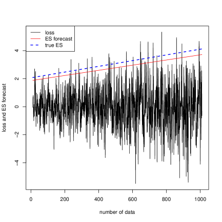
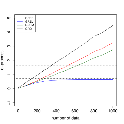
   Figure 1: Realized losses and ES forecasts with a linear extending business (left panel); average log-transformed e-processes obtained by different methods over $1,000$ simulations (right panel)

   We observe from Figure 1 that the GREE e-process dominates the GREL e-process. This is consistent with the result of Theorem 3 by noting the co-movements of the losses and the VaR and ES forecasts which makes the model-free e-statistics $(e_{p}(L_{t},r_{t},z_{t}))_{t\in[n+l]}$ iid.

2. Another example of co-movements between the losses and forecasts is where a company exhibits a non-linear business cycle. Take the random losses to be $L_{t}=Z_{t}(1+\sin(\theta t))$ for $t\in[n+l]$, where $\theta=0.01$. The risk forecasts of $\mathrm{VaR}_{0.95}(L_{t}|\mathcal{F}_{t-1})$ and $\mathrm{ES}_{0.95}(L_{t}|\mathcal{F}_{t-1})$ also have a similar trend but are under-estimated. Namely, we have $z_{t}=1.48(1+\sin(\theta t))$ for VaR and $r_{t}=1.86(1+\sin(\theta t))$ for ES. The losses and forecasts, and the average log e-processes for different methods are plotted in Figure 2.

   

   

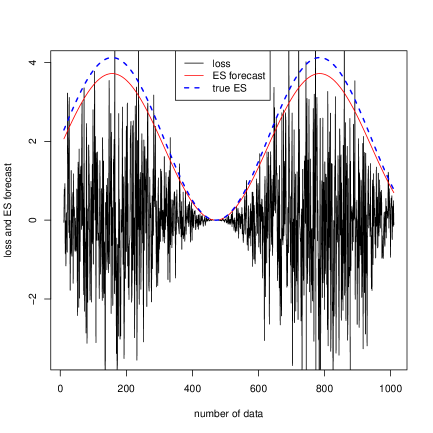
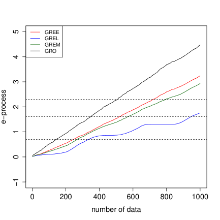
   Figure 2: Realized losses and ES forecasts with a non-linear business cycle (left panel); average log-transformed e-processes obtained by different methods over $1,000$ simulations (right panel)

   Similarly to (i), we also observe better performance of the GREE method than GREL because of the overall iid pattern of the whole e-statistics.

3. It is expected from Theorem 3 that the GREL method will dominate the GREE method when the losses exhibit an iid pattern and there is no clear evidence of co-movements between losses and risk forecasts. Let the random losses be $Z_{1},\dots,Z_{n+l}$; thus, they are iid. Suppose that the risk forecaster announces the forecasts of $\mathrm{VaR}_{0.95}(Z_{t}|\mathcal{F}_{t-1})$ and $\mathrm{ES}_{0.95}(Z_{t}|\mathcal{F}_{t-1})$ to be $z_{t}=1.64+\varepsilon_{t}$ and $r_{t}=2.06+\varepsilon_{t}$, respectively, for $t\in[n+l]$, where $\varepsilon_{1},\dots,\varepsilon_{n+l}$ are iid samples uniformly distributed on the support $\{\pm i/10:i=0,\dots,5\}$. In this case, the forecaster is able to obtain risk forecasts close to the true values but is subject to a forecasting error $(\varepsilon_{t})_{t\in[n+l]}$. Figure 3 plots the realized losses $Z_{t}$, ES forecasts $r_{t}$, and the corresponding e-processes obtained by the GRO, GREE, GREL and GREM methods for $t=l+1,\dots,n+l$.

   

   

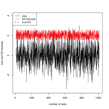
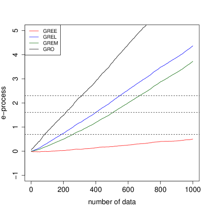
   Figure 3: Realized losses and ES forecasts with iid losses (left panel); average log-transformed e-processes obtained by different methods over $1,000$ simulations (right panel)

   We observe from Figure 3 that the GREL method outperforms the GREE method. This example shows that the GREL method is able to detect evidence against risk forecasts due to downward fluctuations of the forecasts, while GREE does not perform well in this case because it only uses historical forecasts whose average is close to the true value.

5.3 Proof of Theorem 3

We first present a proposition used in the proof of Theorem 3. Its proof is put in Appendix C. This proposition says that under the iid assumption, the betting process computed from empirical distributions is asymptotically equivalent to that computed from the true distribution.

Proposition 3.

Let $X_{1},X_{2},\dots$ be nonnegative iid random variables with $\mathbb{E}[\log(X_{1})]<\infty$. Let

$$\lambda_{t}=\operatorname*{arg\,max}_{\lambda\in[0,\gamma]}\frac{1}{t-1}\sum^{t-1}_{s=1}\log(1-\lambda+\lambda X_{s});\leavevmode\nobreak\ \leavevmode\nobreak\ \lambda^{*}=\operatorname*{arg\,max}_{\lambda\in[0,\gamma]}\mathbb{E}[\log(1-\lambda+\lambda X_{t})],\leavevmode\nobreak\ \leavevmode\nobreak\ t\in\mathbb{N}.$$

We have ${T}^{-1}\sum^{T}_{t=1}(\log(1-\lambda_{t}+\lambda_{t}X_{t}))-\log(1-\lambda^{*}+\lambda^{*}X_{t}))\xrightarrow{L^{1}}0$ as $T\to\infty$.

Proposition 3 gives a simplified illustration of the asymptotic optimality of the GREE method, which uses historical model-free e-statistics as iid input. A rigorous statement of this point is already presented in Theorem 3.

Proof of Theorem 3.

For (i), because $(r_{t},z_{t})_{t\in\mathbb{N}}$ is deterministic and $(e(L_{t},r_{t},z_{t}))_{t\in\mathbb{N}}$ is iid, we have for all $t\in\mathbb{N}$,

$$\lambda^{\mathrm{GRO}}_{t}(r_{t},z_{t})=\operatorname*{arg\,max}_{\lambda\in[0,\gamma]}\mathbb{E}^{Q_{t}}[\log(1-\lambda+\lambda e(L_{t},r_{t},z_{t}))|\mathcal{F}_{t-1}]=\operatorname*{arg\,max}_{\lambda\in[0,\gamma]}\mathbb{E}[\log(1-\lambda+\lambda X_{t})|\mathcal{F}_{t-1}]=:\lambda^{*},$$

where $X_{t}=e(L_{t},r_{t},z_{t})$. The statement thus follows directly from Proposition 3.

For (ii), we first show the result for any fixed $(r,z)\in\psi^{*}(\mathcal{P})$. This follows directly from Proposition 3 by taking $X_{t}=e(L_{t},r,z)$, $\lambda_{t}=\lambda^{\mathrm{GREL}}_{t}(r,z)$, and $\lambda^{*}=\lambda^{\mathrm{GRO}}_{t}(r,z)$ for $t\in\mathbb{N}$.

(a) Suppose that $(r_{t},z_{t})_{t\in\mathbb{N}}$ takes finitely many possible values in $\mathbb{R}^{\mathbb{N}}$. Let $(M_{t})_{t\in\mathbb{N}}$ be defined in (7), $\bm{\lambda}^{\mathrm{GREL}}=(\lambda^{\mathrm{GREL}}_{t}(r_{t},z_{t}))_{t\in\mathbb{N}}$ and $\bm{\lambda}^{\mathrm{GRO}}=(\lambda^{\mathrm{GRO}}(r_{t},z_{t}))_{t\in\mathbb{N}}$. We have

$$\frac{1}{T}(\log(M_{T}(\bm{\lambda}^{\mathrm{GREL}}))-\log(M_{T}(\bm{\lambda}^{\mathrm{GRO}})))\xrightarrow{L^{1}}0$$

by taking mixtures of all possible values of $(r_{t},z_{t})_{t\in\mathbb{N}}$ that are finitely many.

(b) It suffices to show the result for $d=1$ and the general case holds similarly. Since $e(x,r)$ is continuous in $r$ and $r_{t}$, $t\in\mathbb{N}$, are in a common compact set, $e(x,r)$ is uniformly continuous with respect to $r$. Define $M(r,\lambda)=\mathbb{E}^{Q_{t}}[\log(1-\lambda+\lambda e(L_{t},r))|\mathcal{F}_{t-1}]$ with $r\in\mathbb{R}$, $\lambda\in[0,\gamma]$ and $L_{t}\sim Q_{t}$ for $t\in\mathbb{N}$.

Let $Q_{t}$ be the empirical probability measure $\widehat{Q}_{t-1}$ for all $t\in\mathbb{N}$. We now prove that for all $t\in\mathbb{N}$ and $\varepsilon>0$, there exists $\delta_{1}>0$, such that for all $|r-r^{\prime}|<\delta_{1}$, $|\lambda^{\mathrm{GREL}}_{t}(r)-\lambda^{\mathrm{GREL}}_{t}(r^{\prime})|\leqslant\varepsilon$. Suppose that the negated statement is true. Hence there exists $t\in\mathbb{N}$ and $\varepsilon_{0}>0$, such that for all $\delta>0$, there exist $|r_{\delta}-r^{\prime}_{\delta}|<\delta$, $|\lambda^{\mathrm{GREL}}_{t}(r_{\delta})-\lambda^{\mathrm{GREL}}_{t}(r^{\prime}_{\delta})|>\varepsilon_{0}$. Because $\lambda^{\mathrm{GREL}}_{t}(r)=\operatorname*{arg\,max}_{\lambda\in[0,1]}M(r,\lambda)$ and $M(r,\lambda)$ is strictly concave in $\lambda$, we have

$$\min\left\{M(r_{\delta},\lambda^{\mathrm{GREL}}_{t}(r_{\delta}))-M(r_{\delta},\lambda^{\mathrm{GREL}}_{t}(r^{\prime}_{\delta})),\leavevmode\nobreak\ M(r^{\prime}_{\delta},\lambda^{\mathrm{GREL}}_{t}(r^{\prime}_{\delta}))-M(r^{\prime}_{\delta},\lambda^{\mathrm{GREL}}_{t}(r_{\delta}))\right\}>l$$

for some $l>0$. By uniform continuity of $M(r,\lambda)$ with respect to $r$, there exists $\delta_{0}>0$, such that for all $|r-r^{\prime}|<\delta_{0}$,

$$\max\left\{\left|M(r,\lambda^{\mathrm{GREL}}_{t}(r))-M(r^{\prime},\lambda^{\mathrm{GREL}}_{t}(r))\right|,\left|M(r,\lambda^{\mathrm{GREL}}_{t}(r^{\prime}))-M(r^{\prime},\lambda^{\mathrm{GREL}}_{t}(r^{\prime}))\right|\right\}<l.$$

Therefore,

$$2l <M(r_{\delta_{0}},\lambda^{\mathrm{GREL}}_{t}(r_{\delta_{0}}))-M(r_{\delta_{0}},\lambda^{\mathrm{GREL}}_{t}(r^{\prime}_{\delta_{0}}))+M(r^{\prime}_{\delta_{0}},\lambda^{\mathrm{GREL}}_{t}(r^{\prime}_{\delta_{0}}))-M(r^{\prime}_{\delta_{0}},\lambda^{\mathrm{GREL}}_{t}(r_{\delta_{0}}))$$

$$\leqslant\left|M(r_{\delta_{0}},\lambda^{\mathrm{GREL}}_{t}(r_{\delta_{0}}))-M(r^{\prime}_{\delta_{0}},\lambda^{\mathrm{GREL}}_{t}(r_{\delta_{0}}))\right|+\left|M(r_{\delta_{0}},\lambda^{\mathrm{GREL}}_{t}(r^{\prime}_{\delta_{0}}))-M(r^{\prime}_{\delta_{0}},\lambda^{\mathrm{GREL}}_{t}(r^{\prime}_{\delta_{0}}))\right|<2l.$$

This leads to a contradiction.

Similarly, we can show that there exists $\delta_{2}>0$, such that for all $|r-r^{\prime}|<\delta_{2}$, $|\lambda^{\mathrm{GRO}}(r)-\lambda^{\mathrm{GRO}}(r^{\prime})|\leqslant\varepsilon$ by taking $Q_{t}$ to the probability measure $Q$ for the iid random variables $L_{t}$, $t\in\mathbb{N}$. Take $\hat{\delta}=\min\{\delta_{1},\delta_{2}\}$. Because $r_{t}\xrightarrow{\mathrm{p}}r_{0}$, for all $\eta>0$, there exists $N\in\mathbb{N}$, such that $Q(|r_{t}-r_{0}|<\hat{\delta})>1-\eta$ for all $t>N$. It follows that

$$\max\left\{Q(|\lambda^{\mathrm{GREL}}_{t}(r_{t})-\lambda^{\mathrm{GREL}}_{t}(r_{0})|>\varepsilon),\leavevmode\nobreak\ Q(|\lambda^{\mathrm{GRO}}(r_{t})-\lambda^{\mathrm{GRO}}(r_{0})|>\varepsilon)\right\}\leqslant Q(|r_{t}-r_{0}|\geqslant\hat{\delta})<\eta.$$

Since we also have $\lambda^{\mathrm{GREL}}_{t}(r_{0})\xrightarrow{\mathrm{p}}\lambda^{\mathrm{GRO}}(r_{0})$ as $t\to\infty$, it is clear that $\lambda^{\mathrm{GREL}}_{t}(r_{t})\xrightarrow{\mathrm{p}}\lambda^{\mathrm{GRO}}(r_{0})$ and $\lambda^{\mathrm{GRO}}(r_{t})\xrightarrow{\mathrm{p}}\lambda^{\mathrm{GRO}}(r_{0})$ as $t\to\infty$. By boundedness of the betting processes, we have $\lambda^{\mathrm{GREL}}_{t}(r_{t})\xrightarrow{L^{1}}\lambda^{\mathrm{GRO}}(r_{0})$ and $\lambda^{\mathrm{GRO}}(r_{t})\xrightarrow{L^{1}}\lambda^{\mathrm{GRO}}(r_{0})$ as $t\to\infty$. The result thus holds by (C.1).

For (iii), write $\bm{\lambda}^{\mathrm{GREE}}=(\lambda^{\mathrm{GREE}}_{t})_{t\in\mathbb{N}}$ and $\bm{\lambda}^{\mathrm{GREM}}=(\lambda^{\mathrm{GREM}}_{t})_{t\in\mathbb{N}}$. It suffices to notice that $M_{T}(\bm{\lambda}^{\mathrm{GREM}})\geqslant\max\{M_{T}(\bm{\lambda}^{\mathrm{GREL}}),M_{T}(\bm{\lambda}^{\mathrm{GREE}})\}/2$, and by taking a limit as $T\to\infty$ we obtain the asymptotic optimality of $\bm{\lambda}^{\mathrm{GREM}}$ from that of $\bm{\lambda}^{\mathrm{GREE}}$ or $\bm{\lambda}^{\mathrm{GREL}}$. ∎

6 Characterizing model-free e-statistics

In this section, we present several results on the characterization of model-free e-statistics. The main practical message is that the two e-statistics which we introduced, $e_{p}^{Q}$ and $e_{p}^{\mathrm{ES}}$ in Section 2, are essentially the only useful choices for VaR and (ES,VaR), respectively, in building up e-processes in Section 3. The reader more interested in applications may skip this section in the first reading, while keeping in mind the above practical message.

6.1 Necessary conditions for the existence of model-free e-statistics

Not all functionals $\rho$ on $\mathcal{M}$ admit model-free e-statistics that are solely based on the information of $\rho$. Below we give a necessary condition for a model-free e-statistic testing $\rho$ to exist. A functional $\rho:\mathcal{M}\to\mathbb{R}$ is monotone if $\rho(F)\leqslant\rho(G)$ for all $F\leqslant_{1}G$, where $\leqslant_{1}$ is the usual stochastic order; namely, $F\leqslant_{1}G$ if and only if $F\geqslant G$ pointwise on $\mathbb{R}$. We also say that $\rho$ is uncapped if for each $F\in\mathcal{M}$ and $r>\rho(F)$, there exists $\bar{F}\in\mathcal{M}$ such that $\bar{F}\geqslant_{1}F$ and $\rho(\bar{F})=r$. All monetary risk measures (Föllmer and Schied, 2016) are monotone and uncapped. A functional $\rho:\mathcal{M}\to\mathbb{R}$ is quasi-convex if $\rho(\lambda F+(1-\lambda)G)\leqslant\max\{\rho(F),\rho(G)\}$ for all $\lambda\in[0,1]$ and $F,G\in\mathcal{M}$. Similarly, $\rho$ is quasi-concave if $-\rho$ is quasi-convex, and $\rho$ is quasi-linear if it is both quasi-convex and quasi-concave.

Proposition 4.

Suppose that $\rho:\mathcal{M}\to\mathbb{R}$ is monotone and uncapped. If there exists a model-free e-statistic testing $\rho$, then $\rho$ is quasi-convex.

When $\mathcal{M}$ is convex, quasi-convexity of $\rho$ is equivalent to the condition that the set $\{F\in\mathcal{M}:\rho(F)\leqslant r\}$ is convex for each $r\in\mathbb{R}$. The requirement in Proposition 4 rules out a large class of coherent risk measures including ES. As is shown in the following proposition, if the e-statistic testing $\rho$ is strict, then $\rho$ is necessarily quasi-linear, which is stronger than the quasi-convexity in Proposition 4, and this result does not require that $\rho$ is monotone and uncapped.

Proposition 5.

If there exists a model-free e-statistic $e:\mathbb{R}^{2}\to[0,\infty]$ strictly testing $\rho:\mathcal{M}\to\mathbb{R}$, then $\rho$ is quasi-linear.

We say a functional $\rho:\mathcal{M}\to\mathbb{R}$ has convex level sets (CxLS) if the set $\{F\in\mathcal{M}:\rho(F)=r\}$ is convex for each $r\in\mathbb{R}$. Quasi-linearity of $\rho$ is stronger than the condition that $\rho$ has CxLS, and they are equivalent when $\mathcal{M}$ is convex and $\rho$ is monotone. Functionals with CxLS have been studied extensively in the recent literature due to their connection to elicitability and backtesting (Gneiting, 2011; Ziegel, 2016). For a recent summary of related results, see Wang and Wei (2020).

6.2 Characterizing model-free e-statistics for common risk measures

In this section we offer several characterization results of model-free e-statistics for some common risk measures using identification functions. The link between model-free e-statistics and identification functions is presented in Appendix B. The following two propositions characterize all continuous model-free e-statistics testing the mean and for $(\mathrm{var},\mathbb{E})$ testing the variance; see also Examples 1 and 2.

Proposition 6 (Model-free e-statistics for the mean of bounded random variables).

Let $a\in\mathbb{R}$ and $\mathcal{P}$ be the set of distributions in $\mathcal{M}_{1}$ with support in $[a,\infty)$. All continuous $\mathcal{P}$-model-free e-statistics $e^{\prime}$ testing the mean are of the form

$$e^{\prime}(x,r)=1+h(r)\frac{x-r}{r-a},\quad x\geqslant a,\;r\geqslant a,$$

where $h$ is a continuous function on $[a,\infty)$ with $0<h\leqslant 1$. Moreover, the functions $h$ and $r\mapsto(r-a)/h(r)$ are increasing if and only if $e^{\prime}$ is strictly testing the mean.

Proposition 7 (Model-free e-statistics for the variance).

All continuous model-free e-statistics $e^{\prime}$ for $\psi=(\mathrm{var},\mathbb{E})$ testing $\mathrm{var}$ are of the form

$$e^{\prime}(x,r,z)=1+h(r,z)\frac{(z-x)^{2}-r}{r},\quad x,z\in\mathbb{R},\leavevmode\nobreak\ r\geqslant 0,$$

where $h$ is a continuous function on $[0,\infty)\times\mathbb{R}$ with $0<h\leqslant 1$. Moreover, the functions $r\mapsto h(r,z)$ and $r\mapsto$ $r/h(r,z)$ are increasing for all $z\in\mathbb{R}$ if and only if $e^{\prime}$ is strictly testing $\mathrm{var}$.

The simplest model-free e-statistic for $\mathrm{VaR}$ is given in (1) in Example 3. The following proposition exhausts all model-free e-statistics testing $\mathrm{VaR}$ with an additional continuity requirement. We say a model-free e-statistic $e$ is non-conservative if $\int_{\mathbb{R}}e(x,\psi(F))\,\mathrm{d}F(x)=1$ for each $F\in\mathcal{P}$.

Theorem 4 (Model-free e-statistics for VaR).

Let $p\in(0,1)$ and $\mathcal{P}$ be the set of all distributions with a quantile continuous at $p$. All $\mathcal{P}$-model-free e-statistics $e^{\prime}$ that are continuous except at $x=r$, non-conservative, and testing $\mathrm{VaR}_{p}$ are of the form

$$e^{\prime}(x,r)=1+h(r)\frac{p-\mathds{1}_{\{x\leqslant r\}}}{1-p},$$

where $h$ is a continuous function on $\mathbb{R}$ with $0<h\leqslant 1$. The function $h$ is constant if and only if $e^{\prime}$ is strictly testing $\mathrm{VaR}_{p}$.

Next, we consider the model-free e-statistics for $(\mathrm{VaR},\mathrm{ES})$ testing $\mathrm{ES}$. It is straightforward that $\mathrm{ES}_{p}$ is monotone, uncapped, and $\{F\in\mathcal{M}:\mathrm{ES}_{p}(F)\leqslant r\}$ is not convex. Hence, Proposition 4 implies that there does not exist a model-free e-statistic testing $\mathrm{ES}_{p}$ using solely the information of $\mathrm{ES}_{p}$. A similar point was made in Acerbi and Székely (2017) that $\mathrm{ES}_{p}$ is not backtestable in some specific sense. As is shown in Theorem 1, there exists a model-free e-statistic $e^{\mathrm{ES}}_{p}$ testing $\mathrm{ES}_{p}$ using the information of $(\mathrm{ES}_{p},\mathrm{VaR}_{p})$. The following theorem characterizes all model-free e-statistics for $(\mathrm{ES}_{p},\mathrm{VaR}_{p})$ testing $\mathrm{ES}$, which is slightly more than $e^{\mathrm{ES}}_{p}$.

Theorem 5.

Let $p\in(0,1)$ and $\mathcal{P}$ be the set of all distributions with finite mean and a quantile continuous at $p$. All continuous and non-conservative $\mathcal{P}$-model-free e-statistics $e^{\prime}$ for $\left(\mathrm{ES}_{p},\mathrm{VaR}_{p}\right)$ testing $\mathrm{ES}_{p}$ are of the form

$$e^{\prime}(x,r,z)=1+h(r,z)\left(\frac{(x-z)_{+}}{(1-p)(r-z)}-1\right),\quad x\in\mathbb{R},\leavevmode\nobreak\ z<r,$$

where $h$ is a continuous function such that $0<h\leqslant 1$. Moreover, the functions $r\mapsto h(r,z)$ and $r\mapsto$ $(r-z)/h(r,z)$ are increasing for all $z<r$ if and only if $e^{\prime}$ is strictly testing $\mathrm{ES}_{p}$.

Theorems 4 and 5 illustrate the essential roles of $e^{Q}_{p}$ and $e^{\mathrm{ES}}_{p}$ among all possible choices of e-statistics for VaR and the pair (ES,VaR). All choices of e-statistics for $\mathrm{VaR}_{p}$ have the form $1-\lambda+\lambda e_{p}^{Q}(x,r),$ and all those for $(\mathrm{ES}_{p},\mathrm{VaR}_{p})$ has the form $1-\lambda+\lambda e_{p}^{\mathrm{ES}}(x,r,z),$ where $\lambda$ is a function taking values in $[0,1]$. Therefore, in view of (7), the e-statistics $e$ can be without loss of generality chosen as $e^{Q}_{p}$ for $\mathrm{VaR}_{p}$ and $e^{\mathrm{ES}}_{p}$ for $(\mathrm{ES}_{p},\mathrm{VaR}_{p})$, and $\lambda$ can be chosen separately depending on the risk forecasts.

7 Simulation studies

In this section, we provide simulation studies on backtesting the Value-at-Risk and the Expected Shortfall. This illustrates the details of our backtesting methodology numerically. Furthermore, we examine how different factors affect the quality of the backtesting procedure, especially the impact of the choice of the betting process in (7). We evaluate the backtesting performance when the risk measures are under-reported, over-reported, or reported exactly by the risk forecaster.

For all e-tests, we report evidence against the forecasts when the e-process exceeds thresholds $2$, $5$, or $10$. We call such evidence a detection. From the practical viewpoint, the three thresholds we choose form four zones for levels of alerts to financial institutions. This is in a similar sense to the standard three-zone approach for backtesting VaR in the financial industry.

Remark 6.

In classical statistical terminology, what we call a detection is a rejection of the null hypothesis based on our e-test with thresholds $2$, $5$, and $10$, respectively. Our choice of using “detection” here is to emphasize that having detected evidence of moderate size such as $2$ with the e-test is a useful early warning that risk predictions might not be prudent enough. Recall that Jeffrey’s threshold of e-values for “substantial” evidence is 3.2 and for “decisive” evidence is 10; see Shafer (2021) and Vovk and Wang (2021) for more discussions on observing moderately large e-values.

The simulation and data analysis in Sections 7 and 8, together with those in Appendix D, illustrate our main methodology. They are supplemented by extended results and discussions in a separate paper Wang et al. (2022).

7.1 Backtests via stationary time series

We apply our e-backtesting procedure to a setting with time series. For comparison, we use the same setup as in Nolde and Ziegel (2017) and simulate data from an AR$(1)$–GARCH$(1,1)$ process for daily negated log-returns of a financial asset:

$$L_{t}=\mu_{t}+\sigma_{t}Z_{t},\leavevmode\nobreak\ \leavevmode\nobreak\ \mu_{t}=-0.05+0.3X_{t-1},\leavevmode\nobreak\ \leavevmode\nobreak\ \sigma^{2}_{t}=0.01+0.1\varepsilon^{2}_{t-1}+0.85\sigma^{2}_{t-1},\leavevmode\nobreak\ \leavevmode\nobreak\ t\in\mathbb{N}$$

where $\{Z_{t}\}_{t\in\mathbb{N}}$ is a sequence of iid innovations following a skewed-t distribution with shape parameter $\nu=5$ and skewness parameter $\gamma=1.5$. In total, $1,000$ independent simulations are produced, each of which includes a sample of size $500$ used for backtesting. A rolling window of size $500$ is applied for risk estimation at each time spot $t$.

For forecasting, we assume that the data follow an AR$(1)$–GARCH$(1,1)$ process $\{L_{t}\}_{t\in\mathbb{N}}$ with $L_{t}=\mu_{t}+\sigma_{t}Z_{t}$, where $\{Z_{t}\}_{t\in\mathbb{N}}$ is assumed to be a sequence of iid innovations with mean $0$ and variance $1$, following a normal, t-, or skewed-t distribution. Thus, the forecaster has a correct time-series structure with possibly incorrect innovation. Here, $\{\mu_{t}\}_{t\in\mathbb{N}}$ and $\{\sigma_{t}\}_{t\in\mathbb{N}}$ are adapted to $(\mathcal{F}_{t-1})_{t\in\mathbb{N}}$. The details of the forecasting procedure are described in Appendix D.1. The risk forecaster deliberately under-reports, over-reports, or reports the exact point forecasts of ${\mathrm{VaR}}_{p}$ or $(\mathrm{ES}_{p},\mathrm{VaR}_{p})$ she obtains.

For backtesting, the e-processes in (7) are calculated with the betting process $(\lambda_{t})_{t\in[T]}$ chosen by the GREM method using Taylor approximation via (15). The results for the GREE and GREL methods and their comparison are demonstrated in Appendix D.2. We detect evidence against the forecasts when the e-processes exceed thresholds $2$, $5$, or $10$. We first present results for backtesting $\mathrm{VaR}_{0.99}$. The percentage of detections, the average number of days taken to detect evidence against the forecasts (conditional on detection occurring), and the average final log-transformed e-values are shown in Tables 2 and 3.

	normal			t			skewed-t
threshold	$2$	$5$	$10$	$2$	$5$	$10$	$2$	$5$	$10$
$-10\%$	$99.6$	$98.0$	$94.3$	$97.8$	$88.8$	$76.1$	$46.0$	$14.4$	$5.9$
exact	$97.0$	$87.9$	$75.0$	$86.8$	$60.9$	$40.2$	$17.8$	$2.5$	$0.5$
$+10\%$	$86.1$	$62.4$	$41.4$	$62.5$	$26.3$	$11.9$	$6.3$	$0.4$	$0$

Table 2: Percentage of detections ($\%$) for $\mathrm{VaR}_{0.99}$ forecasts over $1,000$ simulations of time series and $500$ trading days using the GREM method

	normal				t				skewed-t
threshold	$2$	$5$	$10$		$2$	$5$	$10$		$2$	$5$	$10$
$-10\%$	$116$	$185$	$228$	$(5.489)$	$156$	$238$	$285$	$(3.390)$	$230$	$284$	$332$	$(0.3707)$
exact	$158$	$239$	$287$	$(3.311)$	$200$	$284$	$322$	$(1.759)$	$219$	$244$	$217$	$(-0.07467)$
$+10\%$	$196$	$277$	$316$	$(1.858)$	$224$	$305$	$351$	$(0.7341)$	$183$	$227$	–	$(-0.2135)$

Table 3: The average number of days taken to detect evidence against $\mathrm{VaR}_{0.99}$ forecasts conditional on detection over $1,000$ simulations of time series and $500$ trading days using the GREM method; numbers in brackets are average final log-transformed e-values

As expected, the results show that evidence against normal and t-innovations is more likely to be detected than against skewed-t innovations, which is the true model. The percentage of detections for exact skewed-t forecasts, or the Type I error, is $0.5\%$ for threshold $10$. Under-reporting VaR leads to earlier detections than reporting the exact VaR forecasts and the converse holds true for over-reporting.

Results on backtests of ES are reported in Tables 4 and 5. The results in Table 4 confirm our intuition that under-reporting or using a wrong innovation can be detected with a large probability, whereas forecasts from the true model and their more conservative versions appear the opposite. Moreover, under-reporting (resp. over-reporting) both of ES and VaR and under-reporting (resp. over-reporting) only ES have similar performance in terms of probability of detection and time of detection. The average time to detection (Table 5) is useful for risk management since early warnings (threshold 2) are often issued after about a fourth of the sampling time, and decisive warnings (threshold 10) after about half of the considered trading days.

	normal			t			skewed-t
threshold	$2$	$5$	$10$	$2$	$5$	$10$	$2$	$5$	$10$
$-10\%$ ES	$99.8$	$99.5$	$98.5$	$98.4$	$88.8$	$77.1$	$47.6$	$16.1$	$6.2$
$-10\%$ both	$99.8$	$99.5$	$98.1$	$98.5$	$91.4$	$82.0$	$48.0$	$15.7$	$6.5$
exact	$99.3$	$95.7$	$88.3$	$88.1$	$63.9$	$43.1$	$18.8$	$4.0$	$0.8$
$+10\%$ both	$95.2$	$80.4$	$61.9$	$64.9$	$27.6$	$9.9$	$7.1$	$1.0$	$0$
$+10\%$ ES	$94.8$	$79.8$	$62.1$	$70.0$	$34.9$	$15.6$	$7.9$	$1.1$	$0.1$

Table 4: Percentage of detections ($\%$) for $\mathrm{ES}_{0.975}$ forecasts over $1,000$ simulations of time series and $500$ trading days using the GREM method

	normal				t				skewed-t
threshold	$2$	$5$	$10$		$2$	$5$	$10$		$2$	$5$	$10$
$-10\%$ ES	$89$	$137$	$176$	$(6.671)$	$151$	$223$	$277$	$(3.428)$	$224$	$271$	$264$	$(0.5072)$
$-10\%$ both	$94$	$146$	$189$	$(6.347)$	$141$	$215$	$271$	$(3.720)$	$218$	$256$	$251$	$(0.4679)$
exact	$129$	$201$	$247$	$(4.311)$	$185$	$267$	$311$	$(1.953)$	$198$	$195$	$251$	$(-0.04676)$
$+10\%$ both	$171$	$250$	$292$	$(2.737)$	$217$	$283$	$289$	$(0.8275)$	$141$	$206$	–	$(-0.2072)$
$+10\%$ ES	$168$	$247$	$297$	$(2.702)$	$207$	$286$	$298$	$(0.9865)$	$147$	$158$	$165$	$(-0.2323)$

Table 5: The average number of days taken to detect evidence against $\mathrm{ES}_{0.975}$ forecasts conditional on detection over $1,000$ simulations of time series and $500$ trading days using the GREM method; “–” represents no detection; numbers in brackets are average final log-transformed e-values

7.2 Monitoring structural change of time series

We examine the power of our e-backtesting method to monitor the structural change of simulated time series data. We refer to Chu et al. (1996) and Berkes et al. (2004) for earlier work on monitoring the structural change of data sets. For a comparison with the results in Hoga and Demetrescu (2022), we use the same setup as described in their Section 6, and call their method the sequential monitoring method. We simulate the losses $\{L_{t}\}_{t\in\mathbb{N}}$ following the GARCH$(1,1)$ process:

$$L_{t}=-\sigma_{t}Z_{t},\leavevmode\nobreak\ \leavevmode\nobreak\ \sigma^{2}_{t}=0.00001+0.04X^{2}_{t-1}+\beta_{t}\sigma^{2}_{t-1},$$

where $\{Z_{t}\}_{t\in\mathbb{N}}$ is a sequence of iid innovations following a skewed-t distribution with shape parameter $\nu=5$ and skewness parameter $\gamma=0.95$, $\beta_{t}=0.7+0.25\mathds{1}_{\{t>b^{*}\}}$ and $b^{*}$ represents the time after which the model is subject to a structural change. We simulate $250$ presampled data for forecasting risk measures and another $250$ data for backtesting.

We choose the probability level for $\mathrm{VaR}_{p}$ and $\mathrm{ES}_{p}$ to be $p=0.95$. Via the presampled data, the forecaster obtains the forecasts of $\mathrm{VaR}_{0.95}(L_{t}|\mathcal{F}_{t-1})$ and $\mathrm{ES}_{0.95}(L_{t}|\mathcal{F}_{t-1})$ using empirical VaR and ES of the residuals and the estimated model parameters $\hat{\bm{\theta}}=(\hat{\omega},\hat{\alpha},\hat{\beta})$. See Appendix D.3 for details of the forecasting procedure. Due to the model-free nature, we only use the losses and forecasts $(L_{t},r_{t},z_{t})$ for our e-backtesting method, while the sequential monitoring method also uses the estimated volatility $\sigma_{t}(\hat{\bm{\theta}})$ by assuming the GARCH model of the losses. As suggested by Hoga and Demetrescu (2022), the Monte Carlo simulations detector with a rolling window performs the best among others for both VaR and ES monitoring. Therefore, we take this method for comparison with ours. We choose the size $m=50$ of the rolling window. The significance level of the sequential monitoring method is set to be $5\%$, while we choose the rejection threshold of our e-backtesting method to be $1/5\%=20$.

Figure 4 plots the average results we get based on $10,000$ simulations, where the betting processes of e-backtesting are chosen by the GREE, GREL or GREM method. The top panels plot the percentage of detections over the total $10,000$ simulations, including those before and after the structural changes at $t=b^{*}+1$, while the bottom panels show the average number of trading days from the structural changes at $t=b^{*}+1$ to detections through backtesting, given that detections occur after $t=b^{*}+1$. We call this quantity the average run length (ARL) as in Hoga and Demetrescu (2022). As expected, all three methods of e-backtesting are dominated by the sequential monitoring method since they do not rely on the model information. However, the GREE, GREL and GREM methods exhibit reasonable performance for all values of $b^{*}$. From the ARL plots, the GREE, GREL and GREM methods detect evidence against the forecasts around $0$ to $30$ days later than the sequential monitoring method. Near $b^{*}=0$ and $b^{*}=250$, the GREE, GREL and GREM methods yield similar detection percentages as the sequential monitoring method.

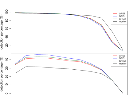
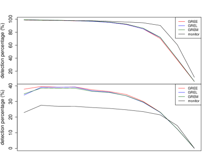
Figure 4: Percentage of detections (%) of $\mathrm{VaR}_{0.95}$ (left panels) and $\mathrm{ES}_{0.95}$ (right panels) forecasts over $10,000$ simulations of time series and $250$ trading days with structural changes at $b^{*}$ (top panels); ARLs of backtesting procedures (bottom panels); black lines (“monitor”) represent the results of the sequential monitoring method

8 Financial data analysis

8.1 The NASDAQ index

We calculate the negated percentage log-returns using data of the NASDAQ Composite index from Jan 16, 1996 to Dec 31, 2021. An AR$(1)$-GARCH$(1,1)$ model is fitted to the data with a moving estimation window of $500$ data points. The e-processes in (7) are calculated with the betting process $(\lambda_{t})_{t\in[T]}$ chosen by the GREE, GREL or GREM method. Different from the backtesting methods used in Section 7.1, for each $t\in[T]$, the empirical mean in (15) is calculated using a moving window of data in the past $500$ days. This choice is made to reflect the practice of risk modeling where more recent data represent better the current market and economic conditions. Therefore, the first $500$ forecasts use $500$ data points each, and we start the backtesting procedure after the first $500$ forecasts are available, thus after the first $1,000$ data points. The sample size for backtesting is $5536$, corresponding to forecasts of risk measures from Jan 3, 2000 to Dec 31, 2021. We plot the negated log-returns and the forecasts of $\mathrm{ES}_{0.975}$ fitted by normal, t-, and skewed-t distributions for the innovations over time in Figure 5. In addition to the parametric methods, we also plot the empirical risk forecasts with a non-parametric rolling window approach in Figure 5.

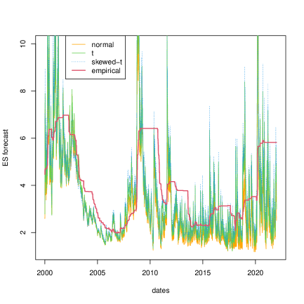
Figure 5: Negated percentage log-returns of the NASDAQ Composite index (left panel); $\mathrm{ES}_{0.875}$ and $\mathrm{ES}_{0.975}$ forecasts fitted by normal distribution (right panel) from Jan 3, 2000 to Dec 31, 2021

We present backtesting results using data from Jan 3, 2005 to Dec 31, 2021 to examine the impact of the 2007 – 2008 financial crisis. Figure 6 shows the e-processes over time. Table 6 demonstrates the average $\mathrm{ES}_{0.975}$ forecasts and the number of days taken to detect evidence against the forecasts, where the second last rows contain the results for ES forecasts deliberately over-reported by $10\%$ assuming skewed-t innovations as a forecasting model that is prudent.

We observe most of the detections in Table 6 happen around $500$ – $700$ trading days after Jan 3, 2005, where significant losses occurred during the financial crisis. Correspondingly, there are sharp jumps of the e-processes in Figure 6 at around $500$ – $700$ trading days. In general, we observe that detections for lower thresholds $2$ and $5$ are significantly earlier than those for the final threshold $10$. This features one of the advantages of our e-backtesting procedure in practice: Our procedure is inherently sequential, and thus, no extra effort is required to allow for monitoring of predictive performance in comparison to testing only at the end of a sampling period. This allows regulators to get alerted much earlier than using the traditional p-tests when e-processes exceed the first threshold $2$ or further exceed $5$. The backtesting procedure may be stopped when an e-process exceeds $10$, which indicates a “decisive” failure of the underlying model used by the financial institution.

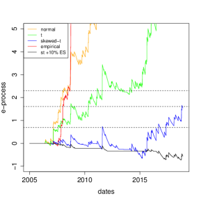
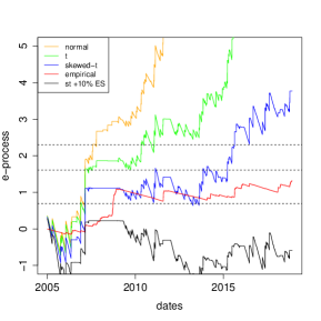
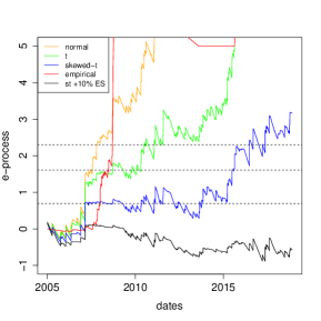
Figure 6: Log-transformed e-processes testing $\mathrm{ES}_{0.975}$ with respect to the number of days for the NASDAQ index from Jan 3, 2005 to Dec 31, 2021; left panel: GREE method, middle panel: GREL method, right panel: GREM method

		GREE				GREL				GREM
threshold		$2$	$5$	$10$		$2$	$5$	$10$		$2$	$5$	$10$
normal	$\mathbf{(2.676)}$	$540$	$704$	$756$		$479$	$540$	$650$		$540$	$610$	$713$
t	$\mathbf{(2.997)}$	$650$	$941$	$1545$		$479$	$540$	$1344$		$540$	$933$	$1381$
skewed-t	$\mathbf{(3.202)}$	$1661$	$3477$	–		$540$	$1545$	$2676$		$540$	$2639$	$2889$
st $+10\%$ $\mathrm{ES}$	$\mathbf{(3.522)}$	–	–	–		–	–	–		–	–	–
empirical	$\mathbf{(3.656)}$	$719$	$758$	$876$		$941$	$3823$	–		$756$	$862$	$931$

Table 6: Average $\mathrm{ES}_{0.975}$ forecasts (boldface in brackets) and the number of days taken to detect evidence against the forecasts for the NASDAQ index from Jan 3, 2005 to Dec 31, 2021; “–” means no detection is detected till Dec 31, 2021

The GREL method performs better than the GREE method in this case except for the empirical forecasts. This may be because the sharp increase of losses upon the occurrence of the financial crisis violates the growth trend and co-movements of the losses and the risk forecasts, making the GREE method not favorable compared with the GREL method as discussed in Example 7. It seems from the result that the GREL method is more likely to detect evidence against the risk forecasts for extreme events (e.g., financial crisis) causing an abnormally sharp increase in losses. The GREL method does not perform well in detecting evidence against the empirical forecasts for both VaR and ES. This is expected because the empirical forecasts and the betting process of the GREL method are both obtained only by the information of the empirical distribution of losses, making GREL lack additional information to reject the empirical forecasts. Compared with the GREE and GREL methods, the performance of the GREM method is more stable in different cases with all cases of underestimation detected. Therefore, the GREM method is recommended as a default choice for implementation.

8.2 Optimized portfolios

Apart from the NASDAQ index, we perform the e-backtesting procedure on data of a portfolio of $n=22$ stocks from Jan 5, 2001 to Dec 31, 2021. Suppose that a bank invests in the above portfolio. After each trading day at time $t\in[T]$, the weights

$$\mathbf{w}_{t}=(w^{1}_{t},\dots,w^{n}_{t})\in\Delta_{n}=\left\{(w_{1},\dots,w_{n})\in[0,1]^{n}:\sum^{n}_{i=1}w_{i}=1\right\}$$

are determined by a mean-variance criterion. Specifically, the bank solves the following optimization problem:

$$\max_{\mathbf{w}_{t}\in\Delta_{n}}\mathbb{E}[-\mathbf{w}_{t}^{\top}\mathbf{L}_{t}]-\frac{\gamma}{2}\mathrm{var}(-\mathbf{w}_{t}^{\top}\mathbf{L}_{t}),$$

where $\mathbf{L}_{t}=(L^{1}_{t},\dots,L^{n}_{t})$ is the vector of negated percentage log-returns for all stocks in the portfolio modeled by an AR$(1)$-GARCH$(1,1)$ process. The bank reports $\mathrm{VaR}$ and $\mathrm{ES}$ of the weighted portfolio by assuming $\mathbf{w}_{t}^{\top}\mathbf{X}_{t}$ to be normal, t-, or skewed-t distributed, respectively. Some of the assumptions in the estimation procedure are simplistic, and hence we do not expect to obtain precise risk forecasts. Suppose that a financial institution reports its risk forecasts based on the naive approach described above. We are more likely to get detections if the simplistic assumptions lead to underestimation. The detailed setup and the list of stocks can be seen in Appendix D.4.

Table 7 shows the average forecasts of $\mathrm{ES}_{0.975}$ and backtesting results with different innovation distributions. The e-processes are plotted in Figure 7. The portfolio data differ from the simulated time series in the sense that the random losses and risk predictions exhibit much more complicated temporal dependence. Detections are obtained in most of the cases for thresholds $2$ and $5$ before large losses come in during the financial crisis in 2008. This demonstrates one of the practical advantages of our method, that is, due to the model-free nature, our e-backtesting method is able to detect evidence against risk forecasts when losses and risk forecasts exhibit complicated temporal dependence. This enables regulations for most real portfolio investments in financial markets, where model assumptions (e.g., stationarity) made by previous literature on backtesting ES are less likely to hold.

		GREE				GREL				GREM
threshold		$2$	$5$	$10$		$2$	$5$	$10$		$2$	$5$	$10$
normal	$\mathbf{(1.224)}$	$547$	$730$	$767$		$438$	$541$	$541$		$461$	$541$	$714$
t	$\mathbf{(1.385)}$	$767$	$934$	$3036$		$1009$	$2207$	$2411$		$778$	$2207$	$2502$
skewed-t	$\mathbf{(1.435)}$	$767$	–	–		$469$	$1009$	$2502$		$541$	$2411$	$2972$
st $+10\%$ $\mathrm{ES}$	$\mathbf{(1.578)}$	–	–	–		–	–	–		–	–	–

Table 7: Average $\mathrm{ES}_{0.975}$ forecasts (boldface in brackets) and the number of days taken to detect evidence against the forecasts for portfolio data from Jan 3, 2005 to Dec 31, 2021; “–” means no detection is detected till Dec 31, 2021

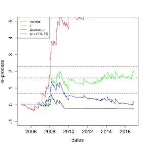
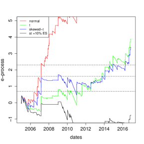
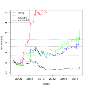
Figure 7: Log-transformed e-processes testing $\mathrm{ES}_{0.975}$ with respect to the number of days for portfolio data from Jan 3, 2005 to Dec 31, 2021; left panel: GREE method, middle panel: GREL method, right panel: GREM method

Between the two methods, the GREL method works better than the GREE method for $\mathrm{ES}_{0.975}$ in most of the cases. However, there is no clear general guidance on which method dominates the other due to the complexity of the strategy, which may not be known. As such, we recommend the GREM method in general.

9 Concluding remarks

The e-backtesting method proposed in this paper is the first model-free and non-asymptotic backtest for ES, the most important risk measure in financial regulation implemented by BCBS (2016). Our methodology contributes to the backtesting issues of ES, which have been a central point of discussions in the risk management literature (e.g., Nolde and Ziegel, 2017; Du and Escanciano, 2017; Hoga and Demetrescu, 2022, and the references therein). Our methods are constructed using the recently developed notions of e-values and e-processes, which are shown to be promising in many application domains of statistics other than risk management. Some topics on which e-values become useful include sequential testing (Shafer, 2021; Grünwald et al., 2020), multiple testing and false discovery control (Vovk and Wang, 2021; Wang and Ramdas, 2022), probability forecast evaluation (Henzi and Ziegel, 2022), meta-analysis in biomedical sciences (ter Schure and Grünwald, 2021), and composite hypotheses (Waudby-Smith and Ramdas, 2022). Our paper connects two active areas of research through theoretical results and methodologies, and we expect more techniques from either world to be applicable to solve problems from the other.

Our e-test procedures feature advantages of e-values, including validity for all stopping times and feasibility for no assumptions on the underlying models. Central to our proposed backtesting method, the notion of model-free e-statistics is introduced, which is useful also for traditional testing problems (Remark 3), although the main focus of the paper is backtesting. The characterization results in Section 6 give guidelines on how to choose model-free e-statistics to build the e-processes. Remarkably, for VaR and ES, the unique forms of model-free e-statistics are identified, leaving little doubt on how to choose them for real-data applications.

If the sample size of a test is fixed, and accurate forecasts for the risk model are available and to be tested together with forecasts for the risk measure, then traditional model-based methods may be recommended to use in practice, as they often have better power than our e-backtests. In the more realistic situations where the sample size is not fixed, or no models are to be tested along with the risk measure forecasts, our e-backtests are useful, and their multifaceted attractive features are illustrated by our study.

As for any other new statistical methodology, e-backtests have their own limitations, challenges, and possible extensions. As the main limitation, since e-backtests require very little information on the underlying model, they could be less powerful than traditional model-based or p-value-based approaches. Therefore, there is a trade-off between flexibility and power that a risk practitioner has to keep in mind. For future directions, an important task is to obtain theoretically optimal betting processes using some data-driven procedures under practical assumptions. The methodology can be extended to more general risk measures and economic indices useful in different contexts, each demanding its own model-free e-statistics and backtesting procedure. Another future direction interesting to us is a game-theoretic framework in which the financial institution actively decides its optimal forecasting strategy by providing the least possible risk forecasts that are barely sufficient to pass a regulatory backtest. The intuition is that, since e-backtests are robust to model assumptions, they should be less vulnerable to this type of adverse strategies of the financial institutions compared to some model-based tests, but a full theoretical analysis is needed before any concrete conclusion can be drawn.

Online Appendices

Appendix A Taylor approximation formulas for GREE and GREL

We give formulas for the betting processes of the GREE and GREL methods for VaR and ES via Taylor approximation. For the GREL method, the special case of VaR, that is, taking $e=e^{Q}_{p}$ in (15), yields

$$\lambda^{\mathrm{GREL}}_{t}\approx 0\vee\frac{(1-p)\left((t-1)p-\sum^{t-1}_{s=1}\mathds{1}_{\{L_{s}\leqslant r\}}\right)}{(t-1)p^{2}+(1-2p)\sum^{t-1}_{s=1}\mathds{1}_{\{L_{s}\leqslant r\}}}\wedge\gamma.$$

For the special case of ES, taking $e=e^{\mathrm{ES}}_{p}$ in (15), the approximation is

$$\lambda_{t}^{\mathrm{GREL}}\approx 0\vee\frac{(1-p)(r-z)\left(\sum^{t-1}_{s=1}(L_{s}-z)_{+}-(t-1)(1-p)(r-z)\right)}{\sum^{t-1}_{s=1}((L_{s}-z)_{+}-(1-p)(r-z))^{2}}\wedge\gamma.$$

The corresponding formulas for the GREE method are obtained by replacing $r$ and $(r,z)$ by $r_{s}$ and $(r_{s},z_{s})$ in the $s$-th summand in above formulas, respectively.

Appendix B Link between model-free e-statistics and identification functions

The link between model-free e-statistics and identification functions is useful for deriving the characterization results of model-free e-statistics in Section 6.2. An integrable function $V:\mathbb{R}^{d+1}\to\mathbb{R}^{d}$ is said to be an $\mathcal{M}$-identification function for a functional $\psi:\mathcal{M}\to\mathbb{R}^{d}$ if $\int_{\mathbb{R}}V(x,\psi(F))\,\mathrm{d}F(x)=\mathbf{0}$ for all $F\in\mathcal{M}$. Furthermore, $V$ is said to be strict if

$$\int_{\mathbb{R}}V(x,y)\,\mathrm{d}F(x)=\mathbf{0}\iff y=\psi(F)$$

for all $F\in\mathcal{M}$ and $y\in\mathbb{R}^{d}$ (Fissler and Ziegel, 2016). We say that $\psi$ is identifiable if there exists a strict $\mathcal{M}$-identification function for $\psi$.

There is a connection between model-free e-statistics strictly testing $\rho$ and identification functions. Let $e:\mathbb{R}^{2}\to\mathbb{R}$ be a model-free e-statistic strictly testing $\rho:\mathcal{M}\to\mathbb{R}$. For $F\in\mathcal{M}$ and $r\geqslant\rho(F)>r^{\prime}$ it holds that

$$\int e(x,r)\,\mathrm{d}F(x)\leqslant 1<\int e(x,r^{\prime})\,\mathrm{d}F(x),$$

and hence, $1-e(x,r)$ is often a strict identification function for $\rho$. Since identifiability of a functional coincides with eliciability under some assumptions detailed in Steinwart et al. (2014), Proposition 5 is not surprising since elicitable functionals are known to have CxLS.

Proposition 8.

Let $e:\mathbb{R}^{d+1}\to[0,\infty]$ be a non-conservative model-free e-statistic for $\psi=(\rho,\phi):\mathcal{M}\to\mathbb{R}^{d}$, and assume that $\phi$ has a $\mathcal{P}$-identification function $v$. We have $V(x,r,z)=(v(x,z),1-e(x,r,z))^{\top}$ is a $\mathcal{P}$-identification function for $\psi$.

Proof.

Let $F\in\mathcal{P}$. By assumption,

$$\int V(x,\rho(F),\phi(F))\,\mathrm{d}F(x)=\left(\int v(x,\phi(F))\,\mathrm{d}F(x),1-\int e(x,\rho(F),\phi(F))\,\mathrm{d}F(x)\right)^{\top}=\mathbf{0}.\qed$$

The connection of model-free e-statistics to identification functions is useful because under some regularity conditions there are characterization results for all possible identification functions for a functional (Fissler, 2017; Dimitriadis et al., 2023). Below, we use these results to derive characterizations of model-free e-statistics. Roughly speaking, given a model-free e-statistic $e$ strictly testing $\rho$, then all other possible model-free e-statistics $e^{\prime}$ strictly testing $\rho$ must be of the form

$$e^{\prime}(x,r)=1+h(r)(e(x,r)-1)$$

for some non-negative function $h$. Clearly, $h$ must fulfill further criteria to ensure that $e^{\prime}$ is a model-free e-statistic strictly testing $\rho$.

A further consequence of these considerations is that for a functional $\rho$ with model-free e-statistic strictly testing $\rho$, there must be an identification function $V(x,r)$ that is bounded below by $-1$. This rules out a number of functionals including the expectation without further conditions on $\mathcal{M}$.

Appendix C Omitted proofs of all results

Proof of Proposition 1.

Suppose that $H_{0}$ in (10) holds. By the VaR-ES relation in (4) and (5),

$$\mathbb{E}[e^{\mathrm{ES}}_{p}(L,r,z)]=\frac{\mathbb{E}\left[(L-z)_{+}\right]}{(1-p)(r-z)}\leqslant\frac{\mathbb{E}\left[(L-\mathrm{VaR}_{p}(L))_{+}\right]}{(1-p)(\mathrm{ES}_{p}(L)-\mathrm{VaR}_{p}(L))}=1.$$

Hence, $e^{\mathrm{ES}}_{p}(L,r,z)$ is an e-variable for (10). ∎

Proof of Proposition 2.

For all $(r,z)\in\mathbb{R}\times\mathbb{R}^{d-1}$ and $t\in\mathbb{N}$, write $X_{t}=e(L_{t},r,z)$.

(i) For the “$\Leftarrow$” direction, suppose that $\lambda^{\mathrm{GRO}}_{t}(r,z)=0$. By Taylor expansion at $\lambda=0$ and continuity of $\lambda\mapsto\mathbb{E}^{Q_{t}}[(X_{t}-1)\lambda|\mathcal{F}_{t-1}]$,

$$\frac{\mathrm{d}}{\mathrm{d}\lambda}\mathbb{E}^{Q_{t}}[\log(1-\lambda+\lambda X_{t})|\mathcal{F}_{t-1}]=\mathbb{E}^{Q_{t}}[(X_{t}-1)|\mathcal{F}_{t-1}]+\mathrm{o}(\lambda).$$

Taking $\lambda\downarrow 0$ yields that $\mathbb{E}^{Q_{t}}[X_{t}|\mathcal{F}_{t-1}]\leqslant 1$. For the “$\Rightarrow$” direction, suppose that $\mathbb{E}^{Q_{t}}[X_{t}|\mathcal{F}_{t-1}]\leqslant 1$. It follows that

$$\mathbb{E}^{Q_{t}}[\log(1-\lambda+\lambda X_{t})|\mathcal{F}_{t-1}]\leqslant\mathbb{E}^{Q_{t}}[(X_{t}-1)\lambda|\mathcal{F}_{t-1}]\leqslant 0.$$

By strict concavity of $\lambda\mapsto\mathbb{E}^{Q_{t}}[\log(1-\lambda+\lambda X_{t})|\mathcal{F}_{t-1}]$, we have $\lambda^{\mathrm{GRO}}_{t}(r,z)=0$, where the upper bound $0$ is obtained.

(ii) For the “$\Leftarrow$” direction, suppose that $\lambda^{\mathrm{GRO}}_{t}(r,z)=1$. It is clear that $Q_{t}(X_{t}=0)=0$. It follows by continuity of $\lambda\mapsto\mathbb{E}^{Q_{t}}[\log(1-\lambda+\lambda X_{t})|\mathcal{F}_{t-1}]$ and $\lambda\mapsto\mathbb{E}^{Q_{t}}[(X_{t}-1)/(1-\lambda+\lambda X_{t})]$ that

$$0\leqslant\left.\frac{\mathrm{d}}{\mathrm{d}\lambda}\mathbb{E}^{Q_{t}}[\log(1-\lambda+\lambda X_{t})|\mathcal{F}_{t-1}]\right|_{\lambda=1}=\mathbb{E}^{Q_{t}}\left[\frac{X_{t}-1}{X_{t}}\middle|\mathcal{F}_{t-1}\right].$$

Hence, $\mathbb{E}^{Q_{t}}[1/X_{t}|\mathcal{F}_{t-1}]\leqslant 1$. For the “$\Rightarrow$” direction, suppose that $\mathbb{E}^{Q_{t}}[1/X_{t}|\mathcal{F}_{t-1}]\leqslant 1$. It follows that

$$\mathbb{E}^{Q_{t}}[\log(1-\lambda+\lambda X_{t})-\log(X_{t})|\mathcal{F}_{t-1}] =\mathbb{E}^{Q_{t}}\left[\log\left(\frac{1-\lambda}{X_{t}}+\lambda\right)\middle|\mathcal{F}_{t-1}\right]$$

$$\leqslant\mathbb{E}^{Q_{t}}\left[(1-\lambda)\left(\frac{1}{X_{t}}-1\right)\middle|\mathcal{F}_{t-1}\right]\leqslant 0.$$

By strict concavity of $\lambda\mapsto\mathbb{E}^{Q_{t}}[\log(1-\lambda+\lambda X_{t})|\mathcal{F}_{t-1}]$, we have $\lambda^{\mathrm{GRO}}_{t}(r,z)=1$, where the upper bound $\log(X_{t})$ is obtained. ∎

The following lemma will be used in the proof of Proposition 3.

Lemma 1.

If $M,M_{t}:[0,1]\to L^{0}$ are convex for all $t\in\mathbb{N}$, $M$ is continuous and $M_{t}(\lambda)\xrightarrow{\mathrm{a.s.}}M(\lambda)$ as $t\to\infty$ for all $\lambda\in[0,1]$, then $\sup_{\lambda\in[0,1]}|M_{t}(\lambda)-M(\lambda)|\xrightarrow{\mathrm{p}}0$ as $t\to\infty$.

Proof.

For all $t\in\mathbb{N}$, define an affine function $\psi_{t}:[0,1]\to L^{0}$ such that $\psi_{t}(0)=M_{t}(0)$ and $\psi_{t}(1)=M_{t}(1)$. This is clear that $\psi_{t}$ converges uniformly to the affine function $\psi:[0,1]\to L^{0}$ such that $\psi(0)=M(0)$ and $\psi(1)=M(1)$. Therefore, replacing $M_{t}$ by $M_{t}-\psi_{t}$ and $M$ by $M-\psi$, we assume without loss of generality that $M_{t}(0)=M(0)=M_{t}(1)=M(1)=0$ for all $t\in\mathbb{N}$.

For all $\eta>0$, take $\varepsilon=\eta/4$. By continuity of $M$, there exists $\delta_{0}>0$, such that $|M(\lambda)-M(\lambda^{\prime})|<\varepsilon$ for all $|\lambda-\lambda^{\prime}|<\delta$. By convexity of $M$, there exists $\tilde{\lambda}\in(0,1)$, such that $M$ is decreasing on $[0,\tilde{\lambda}]$ and increasing on $[\tilde{\lambda},1]$. Define $K=(M(1)-M(\tilde{\lambda}))/(1-\tilde{\lambda})$ and $\delta=\min\{\varepsilon/K,\delta_{0}\}$. There exist $\lambda_{1}<\dots<\lambda_{I-1}$ for $I\in\mathbb{N}\setminus\{1\}$, such that $\lambda_{i+1}-\lambda_{i}<\delta$ for all $i\in\{0,\dots,I-1\}$, where we write $\lambda_{0}=0$ and $\lambda_{I}=1$. It follows that $\delta\leqslant 1-\lambda_{i}$ for all $i\in\{0,\dots,I-1\}$.

Because $M_{t}(\lambda)\xrightarrow{\mathrm{a.s.}}M(\lambda)$ as $t\to\infty$ for all $\lambda\in[0,1]$, there exists an event $A$ with $\mathbb{P}(A)=1$ as follows: There exists $T\in\mathbb{N}$, such that for all $t>T$, we have $|M_{t}(\lambda_{i})-M(\lambda_{i})|<\varepsilon$ for all $i=0,\dots,I$. For all $\lambda\in[0,1]$, there exists $i\in\{0,\dots,I\}$, such that $\lambda\in[\lambda_{i},\lambda_{i+1}]$. Without loss of generality, we assume $0\leqslant\lambda_{i}\leqslant\lambda\leqslant\lambda_{i+1}\leqslant\tilde{\lambda}$. The case of $\tilde{\lambda}\leqslant\lambda_{i}\leqslant\lambda\leqslant\lambda_{i+1}\leqslant 1$ can be shown analogously by symmetry. If $A$ holds, then

$$|M_{t}(\lambda)-M(\lambda)| \leqslant|M_{t}(\lambda)-M(\lambda_{i})|$$

$$<\varepsilon+\frac{M(1)-M(\lambda_{i+1})+\varepsilon}{1-\lambda_{i+1}}\delta+|M(\lambda_{i})-M(\lambda_{i+1})|$$

$$<3\varepsilon+K\min\left\{\frac{\varepsilon}{K},\delta_{0}\right\}\leqslant 4\varepsilon=\eta.$$

Therefore, we have $\mathbb{P}(\sup_{\lambda\in[0,1]}|M_{t}(\lambda)-M(\lambda)|\geqslant\eta)=0$ for all $t>T$. It follows that $\sup_{\lambda\in[0,1]}|M_{t}(\lambda)-M(\lambda)|\xrightarrow{\mathrm{p}}0$ as $t\to\infty$. ∎

Proof of Proposition 3.

Write $M(\lambda)=\mathbb{E}[\log(1-\lambda+\lambda X_{t})]$ and

$$M_{t}(\lambda)=\frac{1}{t-1}\sum^{t-1}_{s=1}\log(1-\lambda+\lambda X_{s})\leavevmode\nobreak\ \leavevmode\nobreak\ \mbox{for }\lambda\in[0,\gamma],\leavevmode\nobreak\ t\in\mathbb{N}.$$

By the strong law of large numbers, we have $M_{t}(\lambda)\xrightarrow{\mathrm{a.s.}}M(\lambda)$ as $t\to\infty$ for all $\lambda\in[0,\gamma]$. Since the functions $M$ and $M_{t}$ are concave for all $t\in\mathbb{N}$, by Lemma 1, we have $\sup_{\lambda\in[0,\gamma]}|M_{t}(\lambda)-M(\lambda)|\xrightarrow{\mathrm{a.s.}}0$. For all $\varepsilon>0$, we have

$$\sup_{\lambda:|\lambda-\lambda^{*}|\geqslant\varepsilon}M(\lambda)\leqslant M(\lambda^{*})$$

by the definition of $\lambda^{*}$ and the concavity of $M$. For all $t\in\mathbb{N}$, we have $M_{t}(\lambda_{t})\geqslant M_{t}(\lambda^{*})$ by the definition of $\lambda_{t}$. Therefore, we have by Theorem 5.7 of van der Vaart (1998) that $\lambda_{t}\xrightarrow{\mathrm{p}}\lambda^{*}$ as $t\to\infty$. Because $\lambda_{t}$ is bounded for all $t\in\mathbb{N}$, $\{\lambda_{t}\}_{t\in\mathbb{N}}$ is uniformly integrable. It follows that $\lambda_{t}\to\lambda^{*}$ with respect to the $L^{1}$-norm as $t\to\infty$, denoted by $\lambda_{t}\xrightarrow{L^{1}}\lambda^{*}$; see e.g., (Resnick, 2019, Theorem 6.6.1).

Next, we show that

$$\frac{1}{T}\sum^{T}_{t=1}(\log(1-\lambda_{t}+\lambda_{t}X_{t})-\log(1-\lambda^{*}+\lambda^{*}X_{t}))\xrightarrow{L^{1}}0$$ (C.1)

as $T\to\infty$. For all $\varepsilon_{1}>0$ and $t\in\mathbb{N}$, by continuity and the monotone convergence theorem, there exists $\delta>0$, such that $\log(1-\delta)>-\varepsilon_{1}$ and $\mathbb{E}[\log(1+(X_{t}-1)\delta)|X_{t}>1]<\varepsilon_{1}$. If $\lambda^{*}=0$, we have $\lambda_{t}\xrightarrow{\mathrm{p}}0$ as $t\to\infty$. Hence, there exists $N>0$, such that for all $t>N$, $\mathbb{P}(\lambda_{t}>\delta)<\varepsilon_{1}$. We write $x_{-}=\min\{x,0\}$ and $x_{+}=\max\{x,0\}$ for $x\in\mathbb{R}$. It follows that

$$\mathbb{E}[\log(1-\lambda_{t}+\lambda_{t}X_{t})_{-}]\geqslant\mathbb{E}[\log(1-\lambda_{t})] \geqslant\log(1-\gamma)\mathbb{P}(\delta<\lambda_{t}\leqslant\gamma)+\log(1-\delta)\mathbb{P}(0\leqslant\lambda_{t}\leqslant\delta)$$

$$\geqslant(\log(1-\gamma)-1)\varepsilon_{1},$$

and

$$\mathbb{E}[\log(1-\lambda_{t}+\lambda_{t}X_{t})_{+}]$$

$$=\mathbb{E}[\log(1-\lambda_{t}+\lambda_{t}X_{t})(\mathds{1}_{\{X_{t}>1,0\leqslant\lambda_{t}\leqslant\delta\}}+\mathds{1}_{\{X_{t}>1,\delta<\lambda_{t}\leqslant\gamma\}})]$$

$$\leqslant\mathbb{E}[\log(1+(X_{t}-1)\delta)|X_{t}>1]\mathbb{P}(0\leqslant\lambda_{t}\leqslant\delta)+\mathbb{E}[\log(1+(X_{t}-1)\gamma)|X_{t}>1]\mathbb{P}(\delta<\lambda_{t}\leqslant\gamma)$$

$$\leqslant(1+\mathbb{E}[\log(1+(X_{t}-1)\gamma)|X_{t}>1])\varepsilon_{1}.$$

It is clear that $\sup_{t\in\mathbb{N}}\mathbb{E}[\log(1+(X_{t}-1)\gamma)|X_{t}>1]$ is bounded because $\sup_{t\in\mathbb{N}}\mathbb{E}[\log(X_{t})]<\infty$. Hence, $\mathbb{E}[|\log(1+\lambda_{t}+\lambda_{t}X_{t})|]<M_{1}\varepsilon_{1}$ for some $M_{1}>0$ and for all $t>N$. Therefore, there exists $N_{1}>0$, such that for all $T>N_{1}$,

$$\mathbb{E}\left[\left|\frac{1}{T}\sum^{T}_{t=1}\log(1-\lambda_{t}+\lambda_{t}X_{t})\right|\right] \leqslant\frac{1}{T}\sum^{N}_{t=1}\mathbb{E}[|\log(1-\lambda_{t}+\lambda_{t}X_{t})|]+\frac{1}{T}\sum^{T}_{t=N+1}\mathbb{E}[|\log(1-\lambda_{t}+\lambda_{t}X_{t})|]$$

$$\leqslant\varepsilon_{1}+\frac{(T-N)M_{1}}{T}\varepsilon_{1}.$$

Hence (C.1) holds for $\lambda^{*}=0$.

If $\lambda^{*}\in(0,\gamma]$, we write $K=\max\{1/\lambda^{*},1/(1-\lambda^{*})\}<\infty$. Thus

$$\frac{X_{t}-1}{1+(X_{t}-1)\lambda^{*}}\in[-K,K]\leavevmode\nobreak\ \leavevmode\nobreak\ \text{for all }t\in\mathbb{N}.$$

For all $\varepsilon_{2}>0$, it is clear by continuity that there exists $\delta>0$, such that $\log(1-\delta/K)>-\varepsilon_{2}$. Because $\lambda_{t}\xrightarrow{L^{1}}\lambda^{*}$ as $t\to\infty$, there exists $N>0$, such that $\mathbb{P}(|\lambda_{t}-\lambda^{*}|>\delta)<\varepsilon_{2}$ and $\mathbb{E}[|\lambda_{t}-\lambda^{*}|]<\varepsilon_{2}$ for all $t>N$. It follows that for all $t>N$,

$$\mathbb{E}\left[(\log(1-\lambda_{t}+\lambda_{t}X_{t})-\log(1-\lambda^{*}+\lambda^{*}X_{t}))_{-}\right]$$

$$=\mathbb{E}\left[\log\left(1+\frac{X_{t}-1}{1+(X_{t}-1)\lambda^{*}}(\lambda_{t}-\lambda^{*})\right)_{-}\right]$$

$$=\mathbb{E}\left[\log\left(1+\frac{X_{t}-1}{1+(X_{t}-1)\lambda^{*}}(\lambda_{t}-\lambda^{*})\right)\left(\mathds{1}_{\{X_{t}\geqslant 1,0\leqslant\lambda_{t}\leqslant\lambda^{*}\}}+\mathds{1}_{\{X_{t}<1,\lambda^{*}<\lambda_{t}\geqslant\gamma\}}\right)\right]$$

$$\geqslant\mathbb{P}(|\lambda_{t}-\lambda^{*}|\leqslant\delta)\log(1-\delta/K)+\mathbb{P}(|\lambda_{t}-\lambda^{*}|>\delta)(\mathbb{E}[\log(1+(X_{t}-1)\lambda_{t})|X_{t}\geqslant 1,0\leqslant\lambda_{t}<\lambda^{*}-\delta]$$

$$+\mathbb{E}[\log(1+(X_{t}-1)\lambda_{t})|X_{t}<1,\lambda^{*}+\delta\leqslant\lambda_{t}<\gamma]-\mathbb{E}[\log(1-\lambda^{*}+\lambda^{*}X_{t})])$$

$$\geqslant(\log(1-\gamma)-\mathbb{E}[\log(1-\lambda^{*}+\lambda^{*}X_{t})]-1)\varepsilon_{2},$$

and

$$\mathbb{E}\left[(\log(1-\lambda_{t}+\lambda_{t}X_{t})-\log(1-\lambda^{*}+\lambda^{*}X_{t}))_{+}\right] =\mathbb{E}\left[\log\left(1+\frac{X_{t}-1}{1+(X_{t}-1)\lambda^{*}}(\lambda_{t}-\lambda^{*})\right)_{+}\right]$$

$$\leqslant K\mathbb{E}[|\lambda_{t}-\lambda^{*}|]<K\varepsilon_{2}.$$

Because $\mathbb{E}[\log(1-\lambda^{*}+\lambda^{*}X_{t})]$ is bounded, we have $E\left[|\log(1-\lambda_{t}+\lambda_{t}X_{t})-\log(1-\lambda^{*}+\lambda^{*}X_{t})|\right]<M_{2}\varepsilon_{2}$ for some $M_{2}>0$ and for all $t>N$. Similar argument as the case of $\lambda^{*}=0$ leads to (C.1). ∎

Proof of Proposition 4.

Let $e$ be a model-free e-statistic testing $\rho$. Write $\mathcal{M}_{r}(\rho)=\{F\in\mathcal{M}:\rho(F)\leqslant r\}$. Take $F,G\in\mathcal{M}_{r}(\rho)$ satisfying $\rho(F)=\rho(G)=r$. We have $\int e(x,r)\,\mathrm{d}F(x)\leqslant 1$ and $\int e(x,r)\,\mathrm{d}G(x)\leqslant 1$, and hence $\int e(x,r)\,\mathrm{d}(\lambda F+(1-\lambda)G)(x)\leqslant 1$. Thus, $\rho(\lambda F+(1-\lambda)G)\leqslant r$. Next, for any $F,G\in\mathcal{M}_{r}(\rho)$, without loss of generality we assume $q:=\rho(F)\geqslant\rho(G)$. Take $\bar{G}\in\mathcal{M}$ such that $\bar{G}\geqslant_{1}G$ and $\rho(\bar{G})=q$. From the above analysis, we know that $\lambda F+(1-\lambda)\bar{G}\in\mathcal{M}_{q}(\rho)\subseteq\mathcal{M}_{r}(\rho)$. Since $\lambda F+(1-\lambda)G\leqslant_{1}\lambda F+(1-\lambda)\bar{G}$, we have $\lambda F+(1-\lambda)G\in\mathcal{M}_{r}(\rho)$. ∎

Proof of Proposition 5.

Take $F,G\in\mathcal{M}$, $r\in\mathbb{R}$, $\lambda\in[0,1]$, and write $H_{\lambda}=\lambda F+(1-\lambda)G$. First, suppose that $\rho(F),\rho(G)\leqslant r$. Since $(x,r)\mapsto e(x,r)$ is decreasing in $r$, we have $\int e(x,r)\,\mathrm{d}F(x)\leqslant 1$ and $\int e(x,r)\,\mathrm{d}G(x)\leqslant 1$, and hence $\int e(x,r)\,\mathrm{d}H_{\lambda}(x)\leqslant 1$ for all $\lambda\in[0,1]$. This implies $\rho(H_{\lambda})\leqslant r$. Further, suppose that $\rho(F),\rho(G)\geqslant r$. Assume that $\rho(H_{\lambda})<r$. Write $q=\rho(H_{\lambda})$. There exists $\varepsilon>0$, such that $q+\varepsilon<r$. Since $(x,r)\mapsto e(x,r)$ is decreasing in $r$, $\int e(x,q+\varepsilon)\,\mathrm{d}H_{\lambda}(x)\leqslant 1$, $\int e(x,q+\varepsilon)\,\mathrm{d}F(x)>1$, and $\int e(x,q+\varepsilon)\,\mathrm{d}G(x)>1$. This leads to a contradiction. Therefore, $\rho(H_{\lambda})\geqslant r$. Summarizing the above arguments, $\rho(F),\rho(G)\leqslant r$ implies $\rho(H_{\lambda})\leqslant r$, and $\rho(F),\rho(G)\geqslant r$ implies $\rho(H_{\lambda})\geqslant r$. This gives the quasi-linearity of $\rho$. ∎

Proof of Proposition 6.

Let $e^{\prime}(x,r)$ be a continuous non-conservative model-free e-statistic testing the mean. By Proposition 8 in Appendix B, $1-e^{\prime}(x,r)$ is an $\mathcal{P}$-identification function for the mean. The function $V(x,r)=x-r$ is a strict $\mathcal{P}$-identification function for the mean which satisfies Dimitriadis et al. (2023, Assumption (S.5)). By Dimitriadis et al. (2023, Theorem S.1), there is a function $\tilde{h}:(a,\infty)\to\mathbb{R}$ such that

$$1-e^{\prime}(x,r)=\tilde{h}(r)(x-r),\quad x\geqslant a,r>a.$$

It is clear that $h(r)=\tilde{h}(r)(r-a)$ has to be continuous. The condition $0\leqslant h\leqslant 1$ arises since $e^{\prime}(x,r)\geqslant 0$. Since $e^{\prime}$ is testing the mean, it has to hold that $h>0$. The condition that $e^{\prime}$ is strictly testing implies the remaining conditions. ∎

Proof of Proposition 7.

Let $e^{\prime}(x,r,z)$ be a continuous non-conservative model-free e-statistic for $(\mathrm{var},\mathbb{E})$ testing $\mathrm{var}$. By Proposition 8 in Appendix B, $(x-z,1-e^{\prime}(x,r,z))^{\top}$ is an $\mathcal{M}_{2}$-identification function for $(\mathrm{var},\mathbb{E})$. The function $V(x,r,z)=(x-z,r-(x-z)^{2})^{\top}$ is a strict $\mathcal{M}_{2}$-identification function for $(\mathrm{var},\mathbb{E})$ which satisfies Dimitriadis et al. (2023, Assumption (S.5)). By Dimitriadis et al. (2023, Theorem S.1), there are functions $h_{1}$ and $h_{2}$ such that

$$e^{\prime}(x,r,z)=1+h_{1}(r,z)(z-x)+h_{2}(r,z)\frac{(z-x)^{2}-r}{r},\quad x,z\in\mathbb{R},\leavevmode\nobreak\ r>0.$$ (C.2)

Since $e^{\prime}$ is continuous, one can see that $h_{2}$ has to be continuous by choosing $x=z$, but then also $h_{1}$ has to be continuous. Putting $t=z-x$ and considering the resulting quadratic function in $t$, one sees that $rh_{1}^{2}(r,z)\leqslant 4h_{2}(r,z)(1-h_{2}(r,z))$ is necessary and sufficient for $e^{\prime}(x,r,z)\geqslant 0$.

For all $r>0$, $z\in\mathbb{R}$, $p\in(0,1)$, and $\varepsilon_{1},\varepsilon_{2}>0$, consider a random variable

$$X=\left(z+\varepsilon_{1}+\left(\frac{r(1-p)}{p}+\frac{\varepsilon_{2}}{p^{2}}\right)^{1/2}\right)\mathds{1}_{A}+\left(z+\varepsilon_{1}-\left(\frac{rp}{1-p}+\frac{\varepsilon_{2}}{(1-p)^{2}}\right)^{1/2}\right)\mathds{1}_{A^{c}},$$

where $A$ is a set with $\mathbb{P}(A)=p$ and $A^{c}$ denotes the complement of $A$. It follows that $\mathbb{E}[X]=z+\varepsilon_{1}$ and $\mathrm{var}(X)=r+\varepsilon_{2}/(p(1-p))>r$. By (C.2) and since $e^{\prime}$ is testing $\mathrm{var}$, we have

$$1<\mathbb{E}[e^{\prime}(X,r,z)] =1+h_{1}(r,z)(z-\mathbb{E}[X])+h_{2}(r,z)\frac{\mathbb{E}[(z-X)^{2}]-r}{r}$$ (C.3)

$$=1-h_{1}(r,z)\varepsilon_{1}+h_{2}(r,z)\left(\frac{\varepsilon^{2}_{1}}{r}+\frac{\varepsilon_{2}}{rp(1-p)}\right).$$

Arbitrariness of $\varepsilon_{1}$ and $\varepsilon_{2}$ yields that $h_{1}\leqslant 0$. Similarly, for all $r>0$, $z\in\mathbb{R}$, $p\in(0,1)$, and $\varepsilon_{1},\varepsilon_{2}>0$, consider the random variable

$$X=\left(z-\varepsilon_{1}+\left(\frac{r(1-p)}{p}+\frac{\varepsilon_{2}}{p^{2}}\right)^{1/2}\right)\mathds{1}_{A}+\left(z-\varepsilon_{1}-\left(\frac{rp}{1-p}+\frac{\varepsilon_{2}}{(1-p)^{2}}\right)^{1/2}\right)\mathds{1}_{A^{c}}.$$

It yields the condition

$$1+h_{1}(r,z)\varepsilon_{1}+h_{2}(r,z)\left(\frac{\varepsilon^{2}_{1}}{r}+\frac{\varepsilon_{2}}{rp(1-p)}\right)>1,$$

which implies that $h_{1}\geqslant 0$. It follows that $h_{1}(r,z)=0$ for all $r>0$ and $z\in\mathbb{R}$. Thus $0=rh_{1}^{2}(r,z)\leqslant 4h_{2}(r,z)\left(1-h_{2}(r,z)\right)$, and thus $0\leqslant h_{2}\leqslant 1$. Since $(\mathbb{E}[(z-X)^{2}]-r)/r>0$ for all $X$ with finite variance, all $z\in\mathbb{R}$ and $r<\mathrm{var}(X)$, the first line of (C.3) yields that $h_{2}>0$. It is also clear that $h_{1}=0$ and $0<h_{2}\leqslant 1$ is sufficient for $e^{\prime}$ to be a model-free e-statistic for $(\mathrm{var},\mathbb{E})$ testing $\mathrm{var}$. Substituting $h_{2}$ by $h$ yields the assertion. The final statement is directly obtained from the same argument as the proof of Proposition 6. ∎

Proof of Theorem 4.

Let $e^{\prime}(x,r)$ be an e-statistic satisfying the stated conditions. By Proposition 8 in Appendix B, $1-e^{\prime}(x,r)$ is a $\mathcal{P}$-identification function for $\mathrm{VaR}_{p}$. The function $\mathds{1}_{\{x\leqslant r\}}-p$ is a strict $\mathcal{P}$-identification function for $\mathrm{VaR}_{p}$ which satisfies Dimitriadis et al. (2023, Assumption (S.5)). By Dimitriadis et al. (2023, Theorem S.1), for any $F\in\mathcal{P}$ it has to hold that

$$\int e^{\prime}(x,r)\,\mathrm{d}F(x)=\int 1+h(r)\frac{p-\mathds{1}_{\{x\leqslant r\}}}{1-p}\,\mathrm{d}F(x).$$

Since $e^{\prime}$ is assumed to be continuous except for points in a set of Lebesgue measure zero, it satisfies Dimitriadis et al. (2023, Assumption (S.7)). All Dirac measures can be approximated by distributions in $\mathcal{P}$ with compact support. Therefore, $\mathcal{P}$ satisfies Dimitriadis et al. (2023, Assumption (S.6)). Together this implies that the stated form of $e^{\prime}$ holds for almost all $(x,r)$. Due to the continuity assumption, we obtain it for all $(x,r)$.

The condition $0\leqslant h\leqslant 1$ ensures that $e^{\prime}(x,r)\geqslant 0$. In order to obtain that $e^{\prime}$ is testing, it is necessary and sufficient that $h>0$. Fix $x\in\mathbb{R}$. For $r\geqslant x$, the function $r\mapsto e^{\prime}(x,r)$ is decreasing if and only if $h$ is increasing; for $r<x$, the same function is decreasing if and only if $h$ is decreasing. Since these considerations hold for any $x\in\mathbb{R}$, $h$ has to be constant. ∎

We first show the following auxiliary lemma for the proof of Theorem 5.

Lemma 2.

Let $p\in(0,1)$ and $\mathcal{P}$ be the set of all distributions with finite mean with a quantile continuous at $p$. All $\mathcal{P}$-model-free e-statistics $e^{\prime}$ for $\left(\mathrm{ES}_{p},\mathrm{VaR}_{p}\right)$ that are non-conservative and continuous except at points with $x=z$ are of the form

$$e^{\prime}(x,r,z)=1+h_{1}(r,z)\frac{\mathds{1}_{\{x\leqslant z\}}-p}{1-p}+h_{2}(r,z)\left(\frac{(x-z)_{+}}{(1-p)(r-z)}-1\right),\quad x\in\mathbb{R},\leavevmode\nobreak\ z<r,$$ (C.4)

where $h_{1},h_{2}$ are continuous functions such that $h_{2}\geqslant 0$ and

$$-1+h_{2}(r,z)\leqslant h_{1}(r,z)\leqslant\frac{1-p}{p}\left(1-h_{2}(r,z)\right),\quad z<r.$$

Proof of Lemma 2.

Let $e^{\prime}(x,r,z)$ be an e-statistic satisfying the stated conditions. By Proposition 8 in Appendix B, $(\mathds{1}_{\{x\leqslant z\}}-p,1-e^{\prime}(x,r,z))^{\top}$ is a $\mathcal{P}$-identification function for $(\mathrm{ES}_{p},\mathrm{VaR}_{p})$, since the function $\mathds{1}_{\{x\leqslant z\}}-p$ is a $\mathcal{P}$-identification function for $\mathrm{VaR}_{p}$. The strict $\mathcal{P}$-identification function $(\mathds{1}_{\{x\leqslant z\}}-p,(x-z)_{+}-(1-p)(r-z))$ for $(\mathrm{ES}_{p},\mathrm{VaR}_{p})$ satisfies Dimitriadis et al. (2023, Assumption (S.5)). With exactly the same arguments as in the proof of Theorem 4, we now obtain (C.4) first in an integrated version, and then pointwise for all $(x,z,r)$ with $z<r$. Considering separately the cases that $x\leqslant z$ and $x>z$, we find that necessary and sufficient conditions for $e^{\prime}(x,r,z)\geqslant 0$ are $h_{2}\geqslant 0$ and $-1+h_{2}\leqslant h_{1}\leqslant((1-p)/p)\left(1-h_{2}\right)$. ∎

Proof of Theorem 5.

Suppose that $(x,r,z)\mapsto e^{\prime}(x,r,z)$ is a model-free e-statistic for $(\mathrm{ES}_{p},\mathrm{VaR}_{p})$ testing $\mathrm{ES}_{p}$ that is non-conservative on $\mathcal{P}$ and continuous except at $x=z$. For all $r\in\mathbb{R}$, $z\leqslant r$, $\varepsilon>0$, and for some $q\in(p,1]$, consider a random variable

$$X=\left((r-z)(1-p)/(1-q)+\varepsilon\right)\mathds{1}_{A}+z,$$

where $\mathbb{P}(A)=1-q$. It follows that $\mathbb{E}[(X-z)_{+}]=(1-p)(r-z)+\varepsilon(1-q)$ and $\mathrm{ES}_{p}(X)=r+\varepsilon(1-q)/(1-p)>r$, since $\mathrm{VaR}_{p}(X)=z$. By Lemma 2, there exist continuous functions $h_{1}$ and $h_{2}$, such that

$$1<\mathbb{E}[e^{\prime}(x,r,z)] =1+h_{1}(r,z)\frac{\mathbb{P}(X\leqslant z)-p}{1-p}+h_{2}(r,z)\left(\frac{\mathbb{E}[(X-z)_{+}]}{(1-p)(r-z)}-1\right)$$ (C.5)

$$=1+h_{1}(r,z)\frac{q-p}{1-p}+h_{2}(r,z)\left(\frac{(1-q)\varepsilon}{(1-p)(r-z)}\right).$$

Arbitrariness of $\varepsilon$ implies that $h_{1}\geqslant 0$ and $h_{2}\geqslant 0$, with at least one of the two inequalities being strict. Similarly, for all $r\in\mathbb{R}$, $z\leqslant r$, $\varepsilon>0$, and for some $q\in[0,p)$, take

$$X=\left(r-z+\varepsilon\right)\mathds{1}_{A}+\varepsilon\mathds{1}_{B}+z,$$

where $\mathbb{P}(A)=1-p$ and $\mathbb{P}(B)=p-q$ and $A\cap B=\varnothing$. We have $\mathbb{E}[(X-z)_{+}]=(1-p)(r-z)+\varepsilon(1-q)$ and $\mathrm{ES}_{p}(X)=r+\varepsilon>r$. Thus, condition (C.5) also has to hold for $q\in[0,p)$, which implies that $h_{1}\leqslant 0$ and $h_{2}\geqslant 0$, with at least one of the two inequalities being strict. According to the previous arguments, we have $h_{1}=0$ and $h_{2}>0$. This implies that $(x,r,z)\mapsto e^{\prime}(x,r,z)$ is also continuous at points with $x=z$. The inequality $-1+h_{2}\leqslant h_{1}\leqslant((1-p)/p)\left(1-h_{2}\right)$ in Lemma 2 yields $h_{2}\leqslant 1$. Substituting $h_{2}$ by $h$ completes the proof. The final statement is obtained by the same argument as the proof of Proposition 6. ∎

Appendix D Supplementary simulation and data analysis

D.1 Forecasting procedure for stationary time series data

This section describes the details of the forecasting procedure for VaR and ES in Section 7.1. We assume that the data generated above follow an AR$(1)$–GARCH$(1,1)$ process $\{L_{t}\}_{t\in\mathbb{N}}$ with $L_{t}=\mu_{t}+\sigma_{t}Z_{t}$, where $\{Z_{t}\}_{t\in\mathbb{N}}$ is assumed to be a sequence of iid innovations with mean $0$ and variance $1$, and $\{\mu_{t}\}_{t\in\mathbb{N}}$ and $\{\sigma_{t}\}_{t\in\mathbb{N}}$ are $\mathcal{F}_{t-1}$-measurable. Specifically, we have

$$\mu_{t}=c+\psi X_{t-1}\leavevmode\nobreak\ \leavevmode\nobreak\ \text{and}\leavevmode\nobreak\ \leavevmode\nobreak\ \sigma^{2}_{t}=\alpha_{0}+\alpha_{1}\varepsilon^{2}_{t-1}+\beta\sigma^{2}_{t-1},\leavevmode\nobreak\ \leavevmode\nobreak\ t\in\mathbb{N}.$$ (D.1)

We first assume the innovations $Z_{t}$ to follow a normal, t-, or skewed-t distribution, and estimate $\{\hat{\mu}_{t}\}_{t\in\mathbb{N}}$ and $\{\hat{\sigma}^{2}_{t}\}_{t\in\mathbb{N}}$ through obtaining the maximum likelihood estimators of $(c,\psi,\alpha_{0},\alpha_{1},\beta)$ under the assumption on the distribution of $Z_{t}$. For t- and skewed-t distributions, parameters are estimated by the maximum likelihood method via the standardized residuals $\{(L_{t}-\hat{\mu}_{t})/\hat{\sigma}_{t}\}_{t\in\mathbb{N}}.$ For a risk measure $\rho$ ($\rho=\mathrm{VaR}_{p}$ or $\rho=\mathrm{ES}_{p}$), the value of $\rho(Z_{t})$ can be calculated explicitly for the assumed parametric models (see e.g., McNeil et al. (2015), Nolde and Ziegel (2017) and Patton et al. (2019)). For estimation, the estimated parameters are plugged into these formulas resulting in estimates $\widehat{\rho(Z_{t})}$. The final risk predictions are then $\hat{\mu}_{t}+\hat{\sigma}_{t}\widehat{\rho(Z_{t})}$, where $\hat{\mu}_{t}$ and $\hat{\sigma}_{t}$ are computed from (D.1) with the estimated parameters. Table D.1 shows the average of the forecasts of $\mathrm{VaR}$ and $\mathrm{ES}$ at different levels over all $1,000$ trials and all trading days, where the last line shows the average forecasts of VaR and ES using the true information of the data generating process.

	$\overline{\mathrm{VaR}}_{0.95}$	$\overline{\mathrm{VaR}}_{0.99}$	$\overline{\mathrm{VaR}}_{0.875}$	$\overline{\mathrm{ES}}_{0.875}$	$\overline{\mathrm{VaR}}_{0.975}$	$\overline{\mathrm{ES}}_{0.975}$
normal	$0.619$	$\mathbf{0.906}$	$0.411$	$\mathbf{0.620}$	$\mathbf{0.752}$	$\mathbf{0.910}$
t	$\mathbf{0.534}$	$\mathbf{0.999}$	$\mathbf{0.300}$	$\mathbf{0.576}$	$\mathbf{0.722}$	$\mathbf{1.065}$
skewed-t	$0.676$	$1.281$	$0.369$	$0.727$	$0.922$	$1.358$
true	$0.674$	$1.271$	$0.368$	$0.723$	$0.918$	$1.343$

Table D.1: Average point forecasts of $\mathrm{VaR}$ and $\mathrm{ES}$ at different levels over $1,000$ simulations of time series and $500$ trading days; values in boldface are underestimated by at least $10\%$ compared with values in the last line

D.2 Comparing GREE and GREL methods for stationary time series

This section serves as a supplement to Section 7.1 by demonstrating the results of backtesting VaR and ES using the GREE and GREL methods through Taylor approximation in (15). Meanwhile, we compare the performance of the GREE and GREL methods. The results of VaR are shown in Tables D.2 and D.3 and those for ES are shown in Tables D.4 and D.5. The GREL method is better than the GREE method in terms of percentage of detections in all cases of VaR and ES. This is consistent with the result in Theorem 3 because for the time series data, the losses used by the GREL method are relatively closer to an iid pattern compared to the whole e-statistics used by the GREE method. This is also not a contradiction to the slightly longer expected time to detection conditional on the detection of the GREL method, noting that the GREL method detects more often.

	GREE
	normal			t			skewed-t
threshold	$2$	$5$	$10$	$2$	$5$	$10$	$2$	$5$	$10$
$-10\%$	$99.0$	$96.5$	$92.1$	$95.5$	$84.2$	$72.4$	$38.3$	$13.7$	$5.6$
exact	$95.0$	$84.4$	$72.0$	$79.5$	$55.4$	$37.2$	$14.0$	$2.8$	$0.8$
$+10\%$	$80.5$	$56.8$	$38.2$	$52.3$	$22.0$	$9.8$	$5.3$	$0.6$	$0$
	GREL
	normal			t			skewed-t
threshold	$2$	$5$	$10$	$2$	$5$	$10$	$2$	$5$	$10$
$-10\%$	$99.7$	$98.3$	$94.5$	$98.2$	$88.7$	$76.7$	$51.0$	$15.1$	$6.6$
exact	$97.8$	$88.6$	$75.9$	$87.4$	$62.4$	$39.8$	$24.3$	$3.2$	$0.6$
$+10\%$	$87.7$	$65.0$	$43.9$	$67.5$	$28.9$	$13.6$	$10.8$	$0.4$	$0.1$

Table D.2: Percentage of detections ($\%$) for $\mathrm{VaR}_{0.99}$ forecasts over $1,000$ simulations of time series and $500$ trading days

	GREE
	normal				t				skewed-t
threshold	$2$	$5$	$10$		$2$	$5$	$10$		$2$	$5$	$10$
$-10\%$	$123$	$186$	$228$	$(5.475)$	$159$	$236$	$278$	$(3.327)$	$206$	$260$	$300$	$(0.2856)$
exact	$164$	$239$	$283$	$(3.236)$	$197$	$272$	$311$	$(1.638)$	$189$	$229$	$265$	$(-0.1012)$
$+10\%$	$197$	$268$	$300$	$(1.734)$	$217$	$280$	$318$	$(0.5933)$	$158$	$224$	–	$(-0.1706)$
	GREL
	normal				t				skewed-t
threshold	$2$	$5$	$10$		$2$	$5$	$10$		$2$	$5$	$10$
$-10\%$	$116$	$185$	$233$	$(5.338)$	$158$	$241$	$293$	$(3.290)$	$239$	$281$	$330$	$(0.3492)$
exact	$160$	$241$	$295$	$(3.240)$	$196$	$286$	$332$	$(1.736)$	$233$	$238$	$289$	$(-0.1463)$
$+10\%$	$189$	$284$	$330$	$(1.849)$	$226$	$304$	$358$	$(0.7599)$	$230$	$211$	$377$	$(-0.3472)$

Table D.3: The average number of days taken to detect evidence against $\mathrm{VaR}_{0.99}$ forecasts conditional on detection over $1,000$ simulations of time series and $500$ trading days; numbers in brackets are average final log-transformed e-values

	GREE
	normal			t			skewed-t
threshold	$2$	$5$	$10$	$2$	$5$	$10$	$2$	$5$	$10$
$-10\%$ ES	$99.7$	$98.9$	$97.9$	$96.7$	$85.6$	$73.8$	$39.9$	$14.9$	$6.1$
$-10\%$ both	$99.8$	$98.9$	$97.3$	$97.9$	$89.2$	$79.3$	$41.1$	$13.6$	$6.4$
exact	$98.6$	$93.2$	$86.1$	$83.0$	$59.8$	$41.1$	$13.5$	$3.2$	$1.1$
$+10\%$ both	$91.1$	$75.7$	$59.8$	$54.2$	$22.3$	$10.2$	$5.1$	$0.8$	$0$
$+10\%$ ES	$91.0$	$76.1$	$60.2$	$60.6$	$28.3$	$13.8$	$6.0$	$1.1$	$0.1$

	GREL
	normal			t			skewed-t
threshold	$2$	$5$	$10$	$2$	$5$	$10$	$2$	$5$	$10$
$-10\%$ ES	$99.9$	$99.2$	$98.2$	$97.5$	$86.2$	$74.1$	$49.3$	$16.6$	$6.5$
$-10\%$ both	$99.9$	$99.0$	$97.6$	$98.1$	$89.2$	$78.8$	$49.9$	$17.4$	$6.6$
exact	$99.2$	$94.6$	$85.7$	$87.6$	$62.4$	$41.9$	$25.3$	$5.6$	$0.9$
$+10\%$ both	$94.1$	$77.3$	$56.2$	$66.0$	$31.6$	$12.5$	$11.5$	$1.5$	$0.1$
$+10\%$ ES	$94.4$	$76.7$	$57.4$	$72.7$	$36.1$	$16.9$	$13.1$	$1.7$	$0.2$

Table D.4: Percentage of detections ($\%$) for $\mathrm{ES}_{0.975}$ forecasts over $1,000$ simulations of time series and $500$ trading days

	GREE
	normal				t				skewed-t
threshold	$2$	$5$	$10$		$2$	$5$	$10$		$2$	$5$	$10$
$-10\%$ ES	$95$	$141$	$181$	$(6.596)$	$158$	$226$	$274$	$(3.365)$	$213$	$250$	$234$	$(0.3991)$
$-10\%$ both	$95$	$152$	$194$	$(6.341)$	$149$	$220$	$269$	$(3.674)$	$207$	$242$	$224$	$(0.3594)$
exact	$139$	$201$	$250$	$(4.278)$	$193$	$265$	$307$	$(1.822)$	$208$	$233$	$220$	$(-0.1011)$
$+10\%$ both	$177$	$249$	$292$	$(2.669)$	$219$	$267$	$286$	$(0.6485)$	$106$	$109$	–	$(-0.1843)$
$+10\%$ ES	$174$	$248$	$295$	$(2.625)$	$210$	$266$	$288$	$(0.8098)$	$90$	$96$	$156$	$(-0.2005)$
	GREL
	normal				t				skewed-t
threshold	$2$	$5$	$10$		$2$	$5$	$10$		$2$	$5$	$10$
$-10\%$ ES	$97$	$147$	$189$	$(6.344)$	$155$	$231$	$282$	$(3.238)$	$235$	$264$	$277$	$(0.4990)$
$-10\%$ both	$99$	$154$	$201$	$(5.963)$	$146$	$221$	$271$	$(3.511)$	$223$	$263$	$278$	$(0.4565)$
exact	$134$	$209$	$258$	$(4.027)$	$191$	$266$	$318$	$(1.892)$	$208$	$233$	$220$	$(-0.09266)$
$+10\%$ both	$174$	$257$	$291$	$(2.577)$	$217$	$289$	$298$	$(0.8661)$	$186$	$207$	$70$	$(-0.3171)$
$+10\%$ ES	$173$	$254$	$296$	$(2.557)$	$215$	$282$	$301$	$(1.007)$	$189$	$185$	$271$	$(-0.3653)$

Table D.5: The average number of days taken to detect evidence against $\mathrm{ES}_{0.975}$ forecasts conditional on detection over $1,000$ simulations of time series and $500$ trading days; “–” represents no detection; numbers in brackets are average final log-transformed e-values

D.3 Forecasting procedure for time series with structural change

This section provides details for the forecasting procedure for time series data with structural change in Section 7.2. After a burn-in period of length $1,000$, $500$ data points are simulated, within which $250$ presampled data $L_{1},\dots,L_{250}$ are for forecasting risk measures and the rest $250$ data $L_{251},\dots,L_{500}$ are for backtesting. The forecaster obtains the estimates $\hat{\bm{\theta}}$ of the model parameters $\bm{\theta}=(\omega,\alpha,\beta_{t})$ once using the standard Gaussian QML for the presampled $250$ losses. For $t\in\{251,\dots,500\}$, the forecasts of $\mathrm{VaR}_{0.95}(L_{t}|\mathcal{F}_{t-1})$ and $\mathrm{ES}_{0.95}(L_{t}|\mathcal{F}_{t-1})$ are obtained by $z_{t}=\sigma_{t}(\hat{\bm{\theta}})\widehat{\mathrm{VaR}}_{0.95}$ and $r_{t}=\sigma_{t}(\hat{\bm{\theta}})\widehat{\mathrm{ES}}_{0.95}$, respectively, where $\widehat{\mathrm{VaR}}_{0.95}$ and $\widehat{\mathrm{ES}}_{0.95}$ are empirical forecasts of VaR and ES using presampled residuals $L_{1}/\sigma_{1}(\hat{\bm{\theta}}),\dots,L_{250}/\sigma_{250}(\hat{\bm{\theta}})$. We choose the size $m=50$ of the rolling window and a leg $d=5$ of autocorrelations.

D.4 Detailed setup of data analysis for optimized portfolios

For the data of optimized portfolios we use in Section 8.2, the first $500$ data points are used for the initial forecast and another $500$ data points are for computing the first value of the betting process of the backtesting procedure. The final sample for backtesting contains $4280$ negated percentage log-returns from Jan 3, 2005 to Dec 31, 2021. The selected stocks are those with the largest market caps in the 11 S&P 500 sectors divided by the GICS level 1 index as of Jan 3, 2005. The list of selected stocks is shown in Table D.6.

Communication Services	Customer Discretionary	Consumer Staples
Verizon Communications Inc.	Time Warner Inc.	The Procter & Gamble Co.
AT&T Inc.	The Home Depot, Inc.	Walmart Inc.
Energy	Financials	Health Care
Exxon Mobil Corp.	Citigroup Inc.	Johnson & Johnson
Chevron Corp.	Bank of America Corp.	Pfizer Inc.
Industrials	Information Technology	Materials
United Parcel Service Inc.	International Business Machines Corp.	EI du Pont de Nemours and Co.
General Electric Co.	Microsoft Corp.	The Dow Chemical Co.
Real Estate	Utilities
Weyerhaeuser Co.	Exelon Corp.
Simon Property Group Inc.	The Southern Co.

Table D.6: 22 selected stocks in S&P 500 sectors divided by GICS level 1 as of Jan 3, 2005 for the portfolio

For forecasting, we assume $L^{i}_{t}=\mu^{i}_{t}+\sigma^{i}_{t}Z^{i}_{t}$ with $\mu^{i}_{t}$ and $\sigma^{i}_{t}$ defined to be the same as (D.1) for all $i\in[n]$. The innovations $\{Z^{i}_{t}\}_{t\in\mathbb{N}}$ are iid with respect to time with mean $0$ and variance $1$ for $i\in[n]$, assumed to be normal, t-, or skewed-t distributed. If a stock delists from the S&P 500 during the period from Jan 3, 2005 to Dec 31, 2021, it is removed from the portfolio as soon as it delists with all of its weight redistributed to the other stocks in the portfolio. The bank reports the $\mathrm{VaR}$ and the $\mathrm{ES}$ of the weighted portfolio by assuming $\mathbf{w}_{t}^{\top}\mathbf{X}_{t}$ to be normal, t-, or skewed-t distributed, respectively, with the mean $\sum^{n}_{i=1}w^{i}_{t}\mu^{i}_{t}$ and the variance $(w^{1}_{t}\sigma^{1}_{t},\dots,w^{n}_{t}\sigma^{n}_{t})^{\top}\Sigma_{t}(w^{1}_{t}\sigma^{1}_{t},\dots,w^{n}_{t}\sigma^{n}_{t})$, where $\Sigma_{t}$ is the covariance matrix of $(Z^{1}_{t},\dots,Z^{n}_{t})$. The assumption is true when the innovations follow the normal distribution or follow the t-distribution with the same degree of freedom. We use this assumption to approximate the true distribution of the portfolio for t-distributions of different degrees of freedom and skewed-t distributions. The parameters of the t- and skewed-t distributions of the weighted portfolio are estimated by the maximum likelihood method assuming the negated percentage log-return of the portfolio to be the AR$(1)$-GARCH$(1,1)$ process with innovations belonging to the same class of distribution. Figure D.1 shows the negated log-returns of the portfolio and the forecasts of $\mathrm{ES}_{0.975}$ over time assuming different innovation distributions.

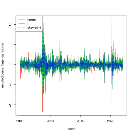
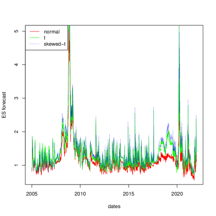
Figure D.1: Portfolio data fitted by different distribution from Jan 3, 2005 to Dec 31, 2021; left panel: negated percentage log-returns, right panel: $\mathrm{ES}_{0.975}$ forecasts

References

- Acerbi and Székely (2014) C. Acerbi and B. Székely. Backtesting Expected Shortfall. Risk Magazine, 27(11):76–81, 2014.
- Acerbi and Székely (2017) C. Acerbi and B. Székely. General properties of backtestable statistics. Preprint, SSRN:2905109, 2017.
- Artzner et al. (1999) P. Artzner, F. Delbaen, J.-M. Eber, and D. Heath. Coherent measures of risk. Mathematical Finance, 9(3):203–228, 1999.
- Bayer and Dimitriadis (2022) S. Bayer and T. Dimitriadis. Regression-based Expected Shortfall backtesting. Journal of Financial Econometrics, 20(3):437–471, 2022.
- BCBS (2013) BCBS. Consultative Document: Fundamental Review of the Trading Book. Bank for International Settlements, 2013. https://www.bis.org/publ/bcbs219.pdf.
- BCBS (2016) BCBS. Minimum Capital Requirements for Market Risk. Bank for International Settlements, 2016. https://www.bis.org/bcbs/publ/d352.pdf.
- Berkes et al. (2004) I. Berkes, E. Gombay, L. Horváth, and P. Kokoszka. Sequential change-point detection in GARCH models. Econometric Theory, 20(6):1140–1167, 2004.
- Berkowitz et al. (2011) J. Berkowitz, P. Christoffersen, and D. Pelletier. Evaluating Value-at-Risk models with desk-level data. Management Science, 57(12):2213–2227, 2011.
- Christoffersen (1998) P. F. Christoffersen. Evaluating interval forecasts. International Economic Review, 39(4):841–862, 1998.
- Christoffersen (2011) P. F. Christoffersen. Elements of Financial Risk Management. Academic Press, second edition, 2011.
- Chu et al. (1996) J. C. S. Chu, M. Stinchcombe, and H. White. Monitoring structural change. Econometrica, 64(5):1045–1065, 1996.
- Clark and McCracken (2001) T. E. Clark and M. W. McCracken. Tests of equal forecast accuracy and encompassing for nested models. Journal of Econometrics, 105(1):85–110, 2001.
- Darling and Robbins (1967) D. A. Darling and H. Robbins. Confidence sequences for mean, variance, and median. Proceedings of the National Academy of Sciences, 58(1):66–68, 1967.
- de la Peña et al. (2004) V. H. de la Peña, M. J. Klass, and T. L. Lai. Self-normalized processes: exponential inequalities, moment bounds and iterated logarithm laws. The Annals of Probability, 32(3):1902–1933, 2004.
- de la Peña et al. (2009) V. H. de la Peña, T. L. Lai, and Q.-M. Shao. Self-Normalized Processes: Limit Theory and Statistical Applications. Probability and Its Applications. Springer, Berlin, first edition, 2009.
- DeMiguel et al. (2009) V. DeMiguel, L. Garlappi, and R. Uppal. Optimal versus naive diversification: How inefficient is the 1/n portfolio strategy? The Review of Financial Studies, 22(5):1915–1953, 2009.
- Diebold and Mariano (1995) F. X. Diebold and R. S. Mariano. Comparing predictive accuracy. Journal of Business & Economic Statistics, 13:253–263, 1995.
- Dimitriadis et al. (2023) T. Dimitriadis, T. Fissler, and J. Ziegel. Osband’s principle for identification functions. Statistical Papers, 2023. doi: https://doi.org/10.1007/s00362-023-01428-x.
- Du and Escanciano (2017) Z. Du and J. C. Escanciano. Backtesting Expected Shortfall: Accounting for tail risk. Management Science, 63(4):940–958, 2017.
- Embrechts et al. (2021) P. Embrechts, T. Mao, Q. Wang, and R. Wang. Bayes risk, elicitability, and the Expected Shortfall. Mathematical Finance, 31(4):1190–1217, 2021.
- Engle and Manganelli (2004) R. F. Engle and S. Manganelli. Caviar: Conditional autoregressive Value at Risk by regression quantiles. Journal of Business & Economic Statistics, 22(4):367–381, 2004.
- Fissler (2017) T. Fissler. On Higher Order Elicitability and Some Limit Theorems on the Poisson and Wiener Space. PhD Thesis, University of Bern, 2017.
- Fissler and Holzmann (2022) T. Fissler and H. Holzmann. Measurability of functionals and of ideal point forecasts. Electronic Journal of Statistics, 16(2):5019–5034, 2022.
- Fissler and Ziegel (2016) T. Fissler and J. F. Ziegel. Higher order elicitability and Osband’s principle. Annals of Statistics, 44(4):1680–1707, 2016.
- Föllmer and Schied (2016) H. Föllmer and A. Schied. Stochastic Finance. De Gruyter, Berlin, fourth edition, 2016.
- Frongillo and Kash (2021) R. Frongillo and I. A. Kash. Elicitation complexity of statistical properties. Biometrika, 108(4):857–879, 2021.
- Giacomini and White (2006) R. Giacomini and H. White. Tests of conditional predictive ability. Econometrica, 74(6):1545–1578, 2006.
- Gneiting (2011) T. Gneiting. Making and evaluating point forecasts. Journal of the American Statistical Association, 106:746–762, 2011.
- Grünwald et al. (2020) P. Grünwald, R. de Heide, and W. M. Koolen. Safe testing. In 2020 Information Theory and Applications Workshop (ITA), pages 1–54. IEEE, 2020.
- Henzi and Ziegel (2022) A. Henzi and J. F. Ziegel. Valid sequential inference on probability forecast performance. Biometrika, 109(3):647–663, 2022.
- Hoga and Demetrescu (2022) Y. Hoga and M. Demetrescu. Monitoring Value-at-Risk and Expected Shortfall forecasts. Management Science, 2022. To appear.
- Jeffreys (1961) H. Jeffreys. Theory of Probability. Oxford University Press, Oxford, third edition, 1961.
- Kelly (1956) J. L. Kelly. A new interpretation of information rate. Bell System Technical Journal, 35(4):917–926, 1956.
- Kupiec (1995) P. Kupiec. Techniques for verifying the accuracy of risk measurement models. Journal of Derivatives, 3(2):73–84, 1995.
- McNeil and Frey (2000) A. J. McNeil and R. Frey. Estimation of tail-related risk measures for heteroscedastic financial time series: An extreme value approach. Journal of Empirical Finance, 7(3–4):271–300, 2000.
- McNeil et al. (2015) A. J. McNeil, R. Frey, and P. Embrechts. Quantitative Risk Management: Concepts, Techniques and Tools. Princeton University Press, Princeton, NJ, revised edition, 2015.
- Nolde and Ziegel (2017) N. Nolde and J. F. Ziegel. Elicitability and backtesting: Perspectives for banking regulation (with discussion). Annals of Applied Statistics, 11(4):1833–1874, 2017.
- Patton et al. (2019) A. Patton, J. F. Ziegel, and R. Chen. Dynamic semiparametric models for Expected Shortfall (and Value-at-Risk). Journal of Econometrics, 211(2):388–413, 2019.
- Ramdas et al. (2022) A. Ramdas, P. Grünwald, V. Vovk, and G. Shafer. Game-theoretic statistics and safe anytime-valid inference. Preprint, arXiv:2210.01948, 2022.
- Resnick (2019) S. Resnick. A Probability Path. Springer, Birkhäuser Boston, MA, first edition, 2019.
- Rockafellar and Uryasev (2002) R. T. Rockafellar and S. Uryasev. Conditional Value-at-Risk for general loss distributions. Journal of Banking & Finance, 26(7):1443–1471, 2002.
- Schmeidler (1989) D. Schmeidler. Subjective probability and expected utility without additivity. Econometrica, 57(3):571–587, 1989.
- Shafer (2021) G. Shafer. The language of betting as a strategy for statistical and scientific communication. Journal of the Royal Statistical Society: Series A, 184(2):407–431, 2021.
- Shafer and Vovk (2019) G. Shafer and V. Vovk. Game-Theoretic Foundations for Probability and Finance. John Wiley & Sons, 2019.
- Shafer et al. (2011) G. Shafer, A. Shen, N. Vereshchagin, and V. Vovk. Test martingales, bayes factors and p-values. Statistical Science, 26(1):84–101, 2011.
- Steinwart et al. (2014) I. Steinwart, C. Pasin, R. Williamson, and S. Zhang. Elicitation and identification of properties. In Proceedings of The 27th Conference on Learning Theory, volume 35 of Proceedings of Machine Learning Research, pages 482–526, Barcelona, Spain, 2014. PMLR.
- ter Schure and Grünwald (2021) J. ter Schure and P. Grünwald. ALL-IN meta-analysis: breathing life into living systematic reviews. Preprint, arXiv:2109.12141, 2021.
- van der Vaart (1998) A. W. van der Vaart. Asymptotic Statistics. Cambridge University Press, Cambridge, 1998.
- Ville (1939) J. Ville. Étude critique de la notion de collectif. Thèses de l’entre-deux-guerres, 1939.
- Vovk and Wang (2020) V. Vovk and R. Wang. Merging sequential e-values via martingales. Preprint, arXiv:2007.06382, 2020.
- Vovk and Wang (2021) V. Vovk and R. Wang. E-values: Calibration, combination, and applications. Annals of Statistics, 49(3):1736–1754, 2021.
- Vovk and Wang (2022) V. Vovk and R. Wang. Efficiency of nonparametric e-tests. arXiv preprint arXiv:2208.08925, 2022.
- Vovk et al. (2022) V. Vovk, B. Wang, and R. Wang. Admissible ways of merging p-values under arbitrary dependence. The Annals of Statistics, 50(1):351–375, 2022.
- Wald (1945) A. Wald. Sequential tests of statistical hypotheses. The Annals of Mathematical Statistics, 16(2):117–186, 1945.
- Wang et al. (2022) Q. Wang, R. Wang, and J. F. Ziegel. Simulation and data analysis for e-backtesting. Preprint, SSRN:4346325, 2022.
- Wang and Ramdas (2022) R. Wang and A. Ramdas. False discovery rate control with e-values. Journal of the Royal Statistical Society, Series B, 84(3):822–852, 2022.
- Wang and Wei (2020) R. Wang and Y. Wei. Risk functionals with convex level sets. Mathematical Finance, 30(4):1337–1367, 2020.
- Wang and Zitikis (2021) R. Wang and R. Zitikis. An axiomatic foundation for the Expected Shortfall. Management Science, 67(3):1413–1429, 2021.
- Wang et al. (2020) R. Wang, Y. Wei, and G. E. Willmot. Characterization, robustness and aggregation of signed Choquet integrals. Mathematics of Operations Research, 45(3):993–1015, 2020.
- Wasserman et al. (2020) L. Wasserman, A. Ramdas, and S. Balakrishnan. Universal inference. Proceedings of the National Academy of Sciences, 117(29):16880–16890, 2020.
- Waudby-Smith and Ramdas (2022) I. Waudby-Smith and A. Ramdas. Estimating means of bounded random variables by betting. Journal of Royal Statistical Society, Series B, 2022. To appear.
- West (1996) K. D. West. Asymptotic inference about predictive ability. Econometrica, 64:1067–1084, 1996.
- Yaari (1987) M. E. Yaari. The dual theory of choice under risk. Econometrica, 55(1):95–115, 1987.
- Ziegel (2016) J. F. Ziegel. Coherence and elicitability. Mathematical Finance, 26(4):901–918, 2016.
- Ziggel et al. (2014) D. Ziggel, T. Berens, G. N. F. Weiß, and D. Wied. A new set of improved Value-at-Risk backtests. Journal of Banking & Finance, 48:29–41, 2014.