A Dataset and Baseline Approach for Identifying Usage States from Non-Intrusive Power Sensing With MiDAS IoT-based Sensors

Abstract

The state identification problem seeks to identify power usage patterns of any system, like buildings or factories, of interest. In this challenge paper, we make power usage dataset available from 8 institutions in manufacturing, education and medical institutions from the US and India, and an initial unsupervised machine learning based solution as a baseline for the community to accelerate research in this area.

1 Introduction

The growth in the deployment of Internet of Things (IoT) sensors across different industries has opened several opportunities for the economy. One of them is the collection of IoT data that companies can use to build smarter solutions. These IoT sensors, while performing their assigned tasks, can also help collect data from real-world objects or devices for analysis and gain intelligence to improve the latter’s capabilities. One such prominent application is the collection and analysis of Electricity Consumption Data (ECD) for a robust and reliable energy management system at any organization.

There is a rich body of work on data-based energy management but much of it is in forecasting and with limited access to data. Accurate forecasting of energy consumption has the potential to save large utility bills. These savings can be realised once the forecasted load knowledge is used to control operations and decisions of the power utility. Mainly in the power systems, the economy of operations and control of operations are sensitive to forecasting errors. Existing forecasting methods can be characterized as conventional (Alfares and Nazeeruddin 2002) or statistical (Tso and Yau 2007) and they focus on short-term load forecasting. These approaches use the trends in the power data to develop a suitable model and use the model for forecasting the future load (Alfares and Nazeeruddin 2002). Based on the characteristics of the time series data, there are different statistical models popularly used. Some of them are auto-regressive (AR), auto-regressive moving-average (ARMA), auto-regressive integrated moving-average (ARIMA). In (Huang and Shih 2003), authors used Gaussian features of the load to determine the model of ARMA dynamically. Complex models can be used to make high-precision predictions, but this is challenging given the high complexity, irregularity, randomness, and non-linearity of real world data. Machine learning techniques can be used to create nonlinear prediction models based on a significant amount of historical data. Typical machine learning models include support vector machines (SVM) (Sapankevych and Sankar 2009) or kernel based classification, artificial neural network (ANN) (Faruk 2010), tree-based ensemble methods such as gradient-boosted regression or decision trees (Ke et al. 2017), long short-term memory units (LSTM) (Bedi and Toshniwal 2020) or transformers (Wen et al. 2022). Authors in (Rajapaksha and Bergmeir 2022) focused on providing rule based explanations for a particular forecast, considering the global forecasting model as a black-box model trained across multi-variate time series.

More recent work in energy management has focused on Non-Intrusive Load Monitoring (NILM) (Batra et al. 2014), (Hart 1992) where, from the aggregate power data, the aim is to dis-aggregate and estimate individual load. This technique is especially appealing to the industry due to its low cost and easy implementation.

Our contribution in this challenge paper for energy management are that we: (a) make a large power usage and harmonics dataset available that is collected using MiDAS sensors from Tantiv4 from 8 institutions in manufacturing, education and medical institutions from the US and India for 15 days, and more days of data available upon request, (b) introduce and describe a generic state identification problem that is of much interest to the industry, and (c) describe an initial un-supervised machine learning based solution to extract different operating states of the power load for a location using current harmonics that can serve as a baseline to the community to accelerate research in this area.

2 State Identification Problem

The objective of state identification (SIP) is to identify power usage patterns of any system, like buildings or factories, of interest. We consider it from the perspective of power systems and as a data analysis problem.

In an electrical system running on AC frequency, any perturbation in the system manifests as an energy spectrum. These spectrum patterns, or signatures, reflects the state in which the system could be: e.g., a factory floor with all machines running normally or a machine beginning to fail due to a fault, or some machines shut for repair; in a datacenter or office, the system under heavy load; or in any industry, an unusual load that the system has not seen till now and needs operator attention. These signatures have traditionally been analyzed as vibration data in a technique commonly referred to as Condition Based Monitoring (Han and Song 2003) which is expensive and intrusive. However, one could alternatively analyze the power data based on electrical current harmonics for states of an electrical system which offers a ’24x7’ monitoring for the different load patterns and faults. This is the true potential of the released data using Machine Learning (ML) and Artificial Intelligence (AI) methods.

As a data analysis problem, we are given a schema $F$ consisting of a list of features $F$ = {$f_{1}$, .. ,$f_{m}$} that a sensor is able to capture. They are also called columns in the data. Adopting the notations of (Goodfellow, Bengio, and Courville 2016) for a classification problem, suppose we are also given a collection of observations $x\in\mathbb{R}^{n}$ corresponding to power usage at a location at a known interval $\Delta$. Each observation, or row in the data, has a structure consistent with $F$. The state identification problem is to produce a function $f$ : $\mathbb{R}^{n}\rightarrow$ {$1$, …, $k$}. When $s$ = $f(x)$, the state corresponding to $x$ is a number capturing the category assigned to the observation. We are interested in the unsupervised SIP problem where $k$ is unknown, i.e., the number of states has to be also learnt.

Apart from solving the SIP problem, a major challenge here is to determine metrics to use for measuring goodness. Due to the high frequency of data collection and resulting data size, getting fully labeled ground truth is infeasible. However, users can contrast significant states and this indicates alternative ways to elicit ground truth.

Location	Industry	Load Illustration	Size of Released Dataset (15-days)	Load Figures (ActivePT vs datetime)*
India-1	Manufacturing	Laser Cutting Machine	ECD - 212MB Harmonics - 3.2GB 5.34% missing data
India-2	Hospital	Main Supply	ECD - 221MB Harmonics - 3.1GB 1.51% missing data
India-3	Manufacturing	Lathe Machine	ECD - 225MB Harmonics - 3.3GB 0.58% missing data
India-4	Manufacturing	Main Supply	ECD - 439MB Harmonics - 3.8GB 10.29% missing data
India-5	Manufacturing	CNC Machine	ECD - 266MB Harmonics - 3.8GB 0.13% missing data
India-6	Manufacturing	Main Supply	ECD - 175MB Harmonics - 2.3GB 0.41% missing data
USA-1	Education	AI/ML Lab	ECD - 393MB Harmonics - 3.4GB 1.67% missing data
USA-2	Education	Data center	ECD - 467MB Harmonics - 3.9GB 1.63% missing data

Table 1: Characteristics of data collected locations; *illustrative power usage for a day - Jul 04 (except India-5: Jul 18, 2022).

3 Data Collection and Usage

We now discuss how the data is collected by the MiDAS device installed by Tantiv4.

MiDAS IoT Sensors:

The MiDAS IOT sensor measures phase voltages (three-phase), phase currents (three-phase), neutral current, power factor (three-phase), active power (three-phase), apparent power (three-phase), reactive power (three-phase), frequency and phase (three-phase) values every 300ms. The device is also capable of collecting three-phases of current and voltage harmonics data from 2 to 32 harmonic levels along with total harmonic distortion for each phase of current and voltage every 500ms. It interfaces using current sensors with a clamp format for easy installation. Voltage sensors are internal to the device. Field terminals can take up to 1.5 sq. mm cables.

Data Collection:

To demonstrate the generality of the SIP problem, we are making datasets available following the FAIR guiding principles (Wilkinson et al. 2016) from different economic industries: Manufacturing, Hospital & Educational institutions. The instructions to obtain the dataset are available here (https://github.com/ai4society/PowerIoT-State-Identification) along with the documentation and the metadata for the released dataset. The GitHub documentation contains a google form link, where the user can fill in the google form and the dataset link can be obtained. The need for the form is that we can inform the user about any data update. The dataset obtained from MiDAS device is of two forms: Electricity Consumption Data and Harmonics Data. The harmonics information obtained by the MiDAS sensor can be used for further analysis of electric device performance.

Electricity Consumption Dataset: contains 28 different features of electricity consumption data. The features are: Current (IA, IB, IC INCURRENT), Voltage (VA, VB, VC), Power Factor (PFA, PFB, PFC, PFT), Phase (PhaseA, PhaseB, PhaseC), Active Power (ActivePA, ActivePB, ActivePC, ActivePT), Reactive Power (ReactivePA, ReactivePB, ReactivePC, ReactivePT), Apparent Power (ApparentPA, ApparentPB, ApparentPC, ApparentPT), Frequency (FREQ), and Time Stamp.

Harmonics Dataset: contains 193 different harmonics data features. The features are: Current (AI_HR[2 to 32], AI_THD, BI_HR[2 to 32], BI_THD, CI_HR[2 to 32], CI_THD), Voltage (AV_HR[2 to 32], AV_THD, BV_HR[2 to 32], BV_THD, CV_HR[2 to 32], CV_THD) and Time Stamp.

The characteristics and the types of different loads present at different locations is shown in Table 1. Active power characteristics plotted for a single weekday for different locations is shown in ’Load Figures’ column in Table 1. Electricity consumption and harmonics data-sets for all of the locations listed in Table 1 are made available online for 15 days for the period July 01, 2022 to July 15, 2022 (except for location India-5: July 16, 2022 to July 31, 2022). The dataset sizes for each location for 15 days are shown in ’Size of the Released Dataset’ column of Table 1. Beyond what is already being released, we have data available for these locations from January-August 2022. So, additional data for more days can be obtained for research purposes by contacting the authors.

• India-1: The sensor is connected to a single Laser cutting machine with power readings between 2 to 25 Amps. The machine laser cuts stainless, carbon steel, aluminum, brass, titanium, and more.

• India-2: The sensor is connected to a hospital’s main incoming supply and the power load includes machines for CT scan, ECG, EEG, Digital Xray, USG, and C-ARM diagnostic services. The power consumption fluctuates between 35 to 110 Amps.

• India-3: The sensor is connected to a single device lathe machine which is used to perform various operations such as cutting, sanding, knurling, drilling, deformation, facing, and turning, with tools that are applied to the work piece to create an object with symmetry about that axis with power consumption between 2 to 40 Amps.

• India-4: The sensor is connected to the main supply of a manufacturing plant which comprises of devices such as multiple CNC (computer numerically controlled) machines, Lathe machines, Lifts etc. and the power consumption is between 15 to 60 Amps.

• India-5: The sensor is connected to a single CNC machine which is used for testing roughness, waviness, flatness, curvature etc of objects and the power consumption is between 3 to 25 Amps.

• India-6: The sensor is connected to the main supply of design & drafting division, comprising of less than 10 employees, equipped with dedicated plotters, jumbo photo copiers, blue printer, spiral binder etc. and the power consumption is between 0.5 to 10 Amps.

• USA-1: The sensor is connected to the main supply of a research center at a University with 10-30 daily users who bring their devices or use servers.

• USA-2: The sensor is connected to the main supply of a server room at a Computer Science department of a University being used for various computational loads.

Data Cleaning and Augmentation:

While working with sensors in the real world, there are often times when data is missing. This can be due to various reasons such as power outage, sensor failure, sensor maintenance work or the sensor is not connected to the network. If one ignores missing data, the quality of analysis, as measured by metrics like accuracy, with them could be degraded. Hence, we employ the optional step of processing it (detailed in code documentation). A user could skip / substitute it with their own methods for cleaning and augmenting the data. In the released data, we filled in a timestamp’s missing data by taking the mean of two previously and subsequently available occurrences of the same timestamp. For example, if the data is missing at 02-01-2022 09:00:00, we looped back(forward) to the previous(future available) dates where the data is available at 09:00:00 timestamp and considered mean of these observations. The main idea of considering the same timestamp is that, given a working environment, the characteristics of the power consumption data for a given timestamp would be similar across the working/non-working days.

4 Initial Solution - Power State Clustering

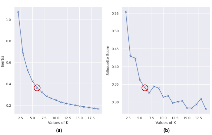
Figure 1: For location India-4 (a) Elbow curve plot with inertia values for different number of clusters (b) Silhouette score plot shows that the optimal number of clusters are 6.

With the help of harmonics data that is being collected by MiDAS sensor, system load performance can be analyzed in depth. This provides more insights regarding the power usage especially in an industrial setting. We will now discuss the power state clustering method that is used to cluster the power usage data into power states using the harmonics data, with the clusters signifying the system states.

4.1 Data Used

The harmonics data collected by the MiDAS sensor consists of 32 harmonic values for three-phases of current and voltage. In our experiment, we have considered the odd harmonics of current for all the three-phases. This feature dataset is sampled at 1 minute frequency. We will use data from India-4 for illustration.

4.2 Finding Number of States For a Location

To classify the different harmonic observations into state categories of system, we must first determine what are the different states that are present in a system for a given time interval. These different system states can be discovered by applying a clustering algorithm over the selected feature dataset.

Clustering Method:

Clustering is a widely used statistical data analysis method in which similar items are grouped into various groups, or more specifically, the data to be analyzed is partitioned into subsets so that the data in each subset are based on a predetermined distance metric (Madhulatha 2012). We experimented with multiple clustering methods (K-Means, DBScan and Agglomerative) and only present the best result obtained with the partition based K-Means.

K-Means Clustering:

is a partitioning based or centroid-based clustering method. Partitioning algorithms work by defining an initial number of groups and then iteratively reallocating items among them to achieve convergence. Typically, this technique selects all clusters simultaneously (Madhulatha 2012).

Determination of optimal number of clusters

Prior to running the clustering algorithm, many clustering techniques require the specification of the number of clusters to be produced in the input data set. Many techniques have been proposed for this problem in literature - one such method is using the elbow curve method. Besides this, we also inspect the quality of clusters using the silhouette score (Shahapure and Nicholas 2020).

Elbow Method:

According to the elbow criterion, one should select the number of clusters such that including another cluster would not provide significantly more additional information (Madhulatha 2012). To chose the optimal number of clusters for a given dataset, we have used the elbow curve method. The sum of the squared distances between the samples and the cluster center is known as inertia. Lower values of inertia indicate that the clusters are well separated. But the inertia becomes 0 once the number of clusters is equal to number of samples. Considering this trade-off between the inertia and the number of clusters, we manually chose the elbow point from the inertia graph. With varying number of clusters from $n=1$ to $n=20$, K-Means algorithm is performed on a 1 week data (January 10, 2022 to January 15, 2022) for each $n$ value and the respective inertia value is calculated. This inertia graph for the respective number of clusters is shown in Figure 1(a). From Figure 1(a), it can be observed that after this elbow point, there is no much change in the inertia value for increasing number of clusters. Hence the elbow point is chosen as the optimal number of clusters. Here the value of optimal number of clusters is falls between 6 to 8.

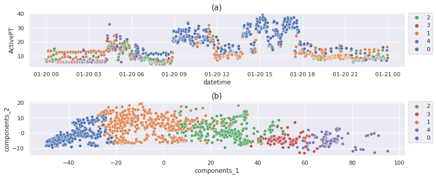
Figure 2: Classifier output for location India-4, January 20, 2022 (Thursday) (a) Clusters (states) viewed with Active Power on Y-axis (b) PCA for 2-dimensional visualization of the clusters (states).

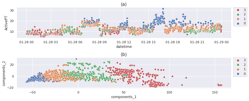
Figure 3: Classifier output for location India-4, January 28, 2022 (Friday) (a) Clusters (states) viewed with Active Power on Y-axis (b) PCA for 2-dimensional visualization of the clusters (states).

Silhouette Score:

The silhouette coefficient is calculated for each data point by $s$ = $\frac{(b-a)}{\max(a,b)}$, where a is the mean intra-cluster distance and b is the mean nearest-cluster distance (Shahapure and Nicholas 2020). Silhouette score is the mean of silhouette coefficient calculated for all the samples. This score ranges from +1 to -1, and the higher the score, the better the clustering. According to the silhouette score analysis and the elbow curve method, it is found that the optimal number of clusters is 6.

Dimentionality Reduction

As we have discussed previously, the data that is being used for clustering consists of 15 features (considering only odd harmonics of current). Visualizing the clusters formed using this high dimensional data is hard to interpret. Therefore, we have used one of the popular dimentionality reduction algorithm, Principle Component Analysis (PCA) (Song, Guo, and Mei 2010). We have extracted two principle components using the PCA algorithm for a 2-dimensional visualisation of the clusters formed.

4.3 Assigning States to Power Data of a Location

Once the different system states are identified for a given time interval, we can build a classification model to classify the collection of observations $x$ into their respective state categories $f(x)$. For this experiment we have used the random forest classifier, which is a tree-based classification algorithm (Breiman 2001). The training dataset comprises of 3 weeks of January (Jan 03, 2022 to Jan 23, 2022). The system state categories are identified using the clustering algorithm and these state categories along with the feature dataset can be used to train a classifier to predict states. We use the random forest classifier for the latter.

We now illustrate the usage of the trained model. In Figure 2 and Figure 3, we show the classification results which correspond to the identified states at the location for two different dates. We note that 5 states were identified in the former for Jan 20 (Thursday) while 4 states are identified in the latter for Jan 28 (Friday). The order of the legend corresponds to the descending order of state labels based on the number of data points clustered into the respective state label. The performance of the classification model is evaluated using F1 score metric. The F1 scores of the system state predictions for the days Jan 20 (Thursday) and Jan 28 (Friday), for which the system labels have been reported in Figure 2 and Figure 3, are 0.51 and 0.67 respectively.

5 Discussion and Challenges

In this paper, we presented a rich dataset of power consumption spanning 8 locations in 3 industries (manufacturing, education and hospital) and two countries (India, US) for 15 days whose size exceeds 27GBs. In addition, more days of data for the same locations from January-August 2022 can be requested for research purposes by contacting the authors.

This data can be used for many energy management applications. While the most studied use-case in literature is energy forecasting for which this data can also be used, we envisage its significant potential while tackling the introduced state identification problem - our second contribution. The SIP problem is driven by industry need.

Furthermore, we described a baseline approach for SIP and presented results for India-4. For this, we performed K-Means clustering by providing the optimal number of clusters as k=6 and the clustering performance is evaluated using the silhouette score metric. These clusters formed can be directly correlated with the system states $f(x)$ for a given collection of observations $x$. Figures 2 and 3 show the different system states obtained from the classification model, trained over the system state labels obtained from the K-Means algorithm, for two different days. Each cluster label in Figures 2 and 3 represents the category to which the system state belongs to. Due to the higher dimensionality of the dataset, we have used PCA to extract two principle components (component_1 and component_2) from the feature dataset. In Figure 2(b), these two principle components are plotted on x-axis and y-axis, respectively, along with the labels obtained for different states from the classification model. We can observe that the different system states are grouped distinctly across the principle component space. The results were validated with domain experts on the ground.

Researchers using our dataset to identify different states of the systems (locations) with their own methods can validate their results by following the documentation provided in the data folder of our GitHub repository and plots in the results folder. This folder contains CSV files with different states identified on each day by location along with their centroid details . The best F1 score of the classification model, by dates, can be found in the leaderboard folder.

Our work opens up many research challenges to the community. First, one needs to handle large data sizes containing time-series and harmonics information, and tackle missing data. Second, one needs to create effective algorithms to identify states in an unsupervised or minimal labeling settings. Third, the methods have to be general across applications and we provided data from three different industries. Fourth, the results should be understandable to the user for which innovations are needed in visualization, interaction and explanation generation. We have begun initial steps towards them (Muppasani et al. 2022; Lakkaraju et al. 2022).

References

- Alfares and Nazeeruddin (2002) Alfares, H. K.; and Nazeeruddin, M. 2002. Electric load forecasting: literature survey and classification of methods. International journal of systems science, 33(1): 23–34.
- Batra et al. (2014) Batra, N.; Kelly, J.; Parson, O.; Dutta, H.; Knottenbelt, W.; Rogers, A.; Singh, A.; and Srivastava, M. 2014. NILMTK: An open source toolkit for non-intrusive load monitoring. In Proc. 5th future energy systems, 265–276; https:// github.com/ nilmtk/nilmtk/blob/master/README.md.
- Bedi and Toshniwal (2020) Bedi, J.; and Toshniwal, D. 2020. Energy load time-series forecast using decomposition and autoencoder integrated memory network. Applied Soft Computing, 93: 106390.
- Breiman (2001) Breiman, L. 2001. Random forests. Machine learning, 45(1): 5–32.
- Faruk (2010) Faruk, D. Ö. 2010. A hybrid neural network and ARIMA model for water quality time series prediction. Engineering applications of artificial intelligence, 23(4): 586–594.
- Goodfellow, Bengio, and Courville (2016) Goodfellow, I.; Bengio, Y.; and Courville, A. 2016. Deep Learning. MIT Press. http://www.deeplearningbook.org.
- Han and Song (2003) Han, Y.; and Song, Y. 2003. Condition monitoring techniques for electrical equipment-a literature survey. IEEE Transactions on Power delivery, 18(1): 4–13.
- Hart (1992) Hart, G. W. 1992. Nonintrusive appliance load monitoring. Proceedings of the IEEE, 80(12): 1870–1891.
- Huang and Shih (2003) Huang, S.-J.; and Shih, K.-R. 2003. Short-term load forecasting via ARMA model identification including non-Gaussian process considerations. IEEE Transactions on power systems, 18(2): 673–679.
- Ke et al. (2017) Ke, G.; Meng, Q.; Finley, T.; Wang, T.; Chen, W.; Ma, W.; Ye, Q.; and Liu, T.-Y. 2017. Lightgbm: A highly efficient gradient boosting decision tree. Proc. Advances in neural information processing systems, 30.
- Lakkaraju et al. (2022) Lakkaraju, K.; Palaiya, V.; Paladi, S. T.; Appajigowda, C.; Srivastava, B.; and Johri, L. 2022. Data-Based Insights for the Masses: Scaling Natural Language Querying to Middleware Data. In Proc. Database Sys. Adv. App. (DASFAA).
- Madhulatha (2012) Madhulatha, T. S. 2012. An overview on clustering methods. arXiv preprint arXiv:1205.1117.
- Muppasani et al. (2022) Muppasani, B. C.; Anand, C. J.; Appajigowda, C.; Srivastava, B.; and Johri, L. 2022. Power Forecasting and Anomaly Detection with MIDAS IoT-based Sensor. In DOI: 10.13140/RG.2.2.17358.33600.
- Rajapaksha and Bergmeir (2022) Rajapaksha, D.; and Bergmeir, C. 2022. LIMREF: Local Interpretable Model Agnostic Rule-based Explanations for Forecasting, with an Application to Electricity Smart Meter Data. arXiv preprint arXiv:2202.07766.
- Sapankevych and Sankar (2009) Sapankevych, N. I.; and Sankar, R. 2009. Time series prediction using support vector machines: a survey. IEEE computational intelligence magazine, 4(2): 24–38.
- Shahapure and Nicholas (2020) Shahapure, K. R.; and Nicholas, C. 2020. Cluster quality analysis using silhouette score. In 2020 IEEE 7th Intl Conf. Data Science and Advanced Analytics (DSAA).
- Song, Guo, and Mei (2010) Song, F.; Guo, Z.; and Mei, D. 2010. Feature selection using principal component analysis. In 2010 international conference on system science, engineering design and manufacturing informatization, volume 1, 27–30. IEEE.
- Tso and Yau (2007) Tso, G. K.; and Yau, K. K. 2007. Predicting electricity energy consumption: A comparison of regression analysis, decision tree and neural networks. Energy, 32(9): 1761–1768.
- Wen et al. (2022) Wen, Q.; Zhou, T.; Zhang, C.; Chen, W.; Ma, Z.; Yan, J.; and Sun, L. 2022. Transformers in Time Series: A Survey. In arXiv:2202.07125.
- Wilkinson et al. (2016) Wilkinson, M. D.; Dumontier, M.; Aalbersberg, I. J.; Appleton, G.; Axton, M.; Baak, A.; Blomberg, N.; Boiten, J.-W.; da Silva Santos, L. B.; Bourne, P. E.; et al. 2016. The FAIR Guiding Principles for scientific data management and stewardship. Scientific data, 3(1): 1–9.