Finite temperature tensor network study of
the Hubbard model on an infinite square lattice
Abstract
The Hubbard model is a longstanding problem in the theory of strongly correlated electrons and a very active one in the experiments with ultracold fermionic atoms. Motivated by current and prospective quantum simulations, we apply a two-dimensional tensor network—an infinite projected entangled pair state—evolved in imaginary time by the neighborhood tensor update algorithm working directly in the thermodynamic limit. With symmetry and the bond dimensions up to 29, we generate thermal states down to the temperature of times the hopping rate. We obtain results for spin and charge correlators, unaffected by boundary effects. The spin correlators—measurable in prospective ultracold atoms experiments attempting to approach the thermodynamic limit—provide evidence of disruption of the antiferromagnetic background with mobile holes in a slightly doped Hubbard model. The charge correlators reveal the presence of hole-doublon pairs near half filling and signatures of hole-hole repulsion on doping. We also obtain specific heat in the slightly doped regime.
I The Hubbard model
One of the simplest models of interacting fermions on a lattice is the Fermi Hubbard model (FHM) with on-site repulsion between electrons of opposite spins:
| (1) | |||||
Here annihilates an electron with spin at site , is the number operator, , repulsion strength , and is the chemical potential. Here denotes summation over nearest-neighbor (NN) sites on a square lattice with hopping energy . Although FHM is deemed to be an inordinately simple model for describing real materials, the competition between and gives rise to a myriad of physical phenomena, including stripe phases and Mott insulator. The model has exact solutions for some limits in one dimension [1, 2]. However, obtaining thermodynamic results for a two-dimensional (2D) system is exceedingly challenging, even with the most sophisticated numerical techniques, see [3] for a recent review.
On the experimental front, ultracold atoms serve as a simulation platform where one can realize condensed matter physics models with high tunability [4, 5, 6], including FHM [7, 8, 9, 10, 11, 12, 13, 14]. Quantum gas microscopy [15, 16, 17, 18] promises manipulations of individual atoms in optical lattices with faithful spin and density readouts, and have achieved impressive success in simulation of the many-body physics of fermions with alkali, potassium, and lithium isotopes [19, 20, 21, 22]. Soon followed single-site resolved detection of 2D Fermi-Hubbard physics encompassing imaging of antiferromagnetic correlations [23, 24, 25, 26, 27], entanglement entropy [28, 29, 30, 31], hidden string order and magnetic polarons [32, 33, 34, 35]. These experiments mostly use harmonically confined systems of tens of fermions and can reach temperatures down to .
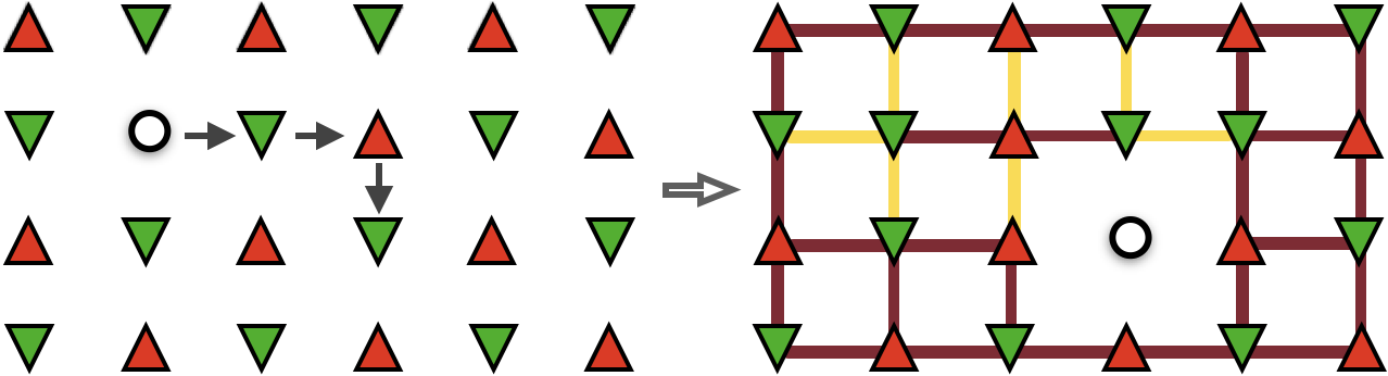
In FHM with low doping, a hole moving in an anti-ferromagnetic (AFM) background leaves a track of ferromagnetically bound bubbles known as magnetic polarons, see Fig. 1. Direct experimental detection of magnetic polarons [33] has fuelled several recent experimental and numerical/theoretical efforts [36, 37, 38, 39, 40, 41, 42, 43, 44, 45]. The latter frequently resort to the effective model [46], or study a rather particular single-hole doping limit. Our work provides results for finite temperature spin and charge correlations for the 2D FHM directly in the thermodynamic limit. It is in line with recent experimental efforts to push quantum simulation of FHM towards the same limit by trapping hundreds of ultracold atoms in a box-like potential [35].
Here we consider and an average electron density per site and , which correspond to doping and , respectively. For these values, FHM captures essential aspects of high- superconductors such as the stripe phases [47, 48, 49], although additional terms such as next NN hopping might be necessary to stabilize the superconducting phase [50] and further additional bands for fluctuating stripes at finite temperature [51]. In the following, we set as a unit of energy. The temperature is measured in these units ().
II Tensor networks
Quantum condensed matter states hosted by two-dimensional lattices can often be efficiently represented by a type of tensor networks (TN) [52, 53] known as the infinite projected entangled-pairs state (iPEPS) ansatz [54, 55, 56]. It is a state-of-the art numerical method for strongly correlated systems [57, 58, 59, 60]. The iPEPS was instrumental in solving the long-standing magnetization plateaus problem in the highly frustrated compound [61, 62], establishing the striped nature of the ground state of the doped 2D Hubbard model [47], and providing new evidence for gapless spin liquid in the kagome Heisenberg antiferromagnet [63, 64]. Further technical progress [65, 66, 67, 68, 69, 70, 71, 72, 73] paved the way towards even more challenging problems, including simulation of thermal states [74, 75, 76, 77, 78, 79, 80, 81, 82, 83, 84, 85, 86, 87, 88]. Very recently there has been promising advancements to calculate the ground states of three-dimensional systems [89]. The alternative tensor-network-based approach considers systems on cylinders and is now routinely used to investigate 2D ground states using density matrix renormalization group (DMRG) [47, 90] and was also applied to thermal states [91, 92, 93, 94, 95, 96, 48]. It is, nevertheless, severely limited by the exponential growth of the bond dimension with system’s width. Furthermore, tensor network approaches relying on contraction of a 3D tensor network representing a 2D thermal state have been proposed [97, 98, 99, 100, 101, 102, 103, 104].
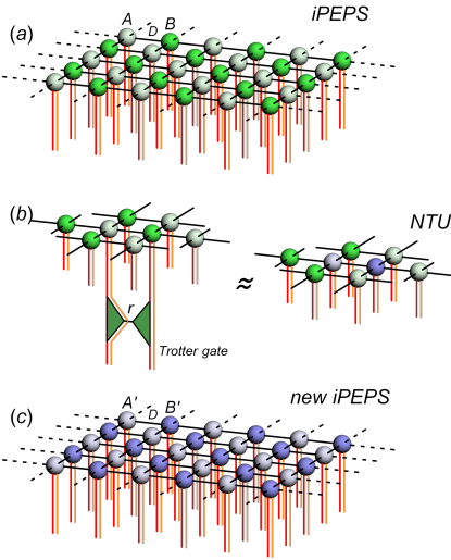
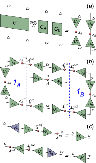
In this paper, we apply iPEPS with abelian symmetries(see Appendix A for brief description) to the 2D Hubbard model at finite temperature. We perform direct imaginary time evolution of an iPEPS that represents purification of the thermal state [82], see Fig. 2(a). For the sake of its numerical stability, we use a fermionic version of the neighborhood tensor update (NTU) algorithm [105], implementing the symmetry and further refinements. We enforce fermionic statistics by following a general scheme of Refs. [106, 107]. The latter include the spatially and rotationally invariant assignment of symmetry sectors’ bond dimensions of the tensors (FIX) and an environment-assisted truncation (EAT) procedure which makes the Trotter step of the NTU algorithm better aware of its tensor environment. We provide detailed descriptions of FIX and EAT in Appendix C. We calculate two-point spin and charge correlators for inverse temperatures . These results are well converged in the iPEPS bond dimension and, by construction, they are free of finite-size effects. This range of temperatures is accessible for current ultracold atoms experiments attempting to reach the thermodynamic limit.
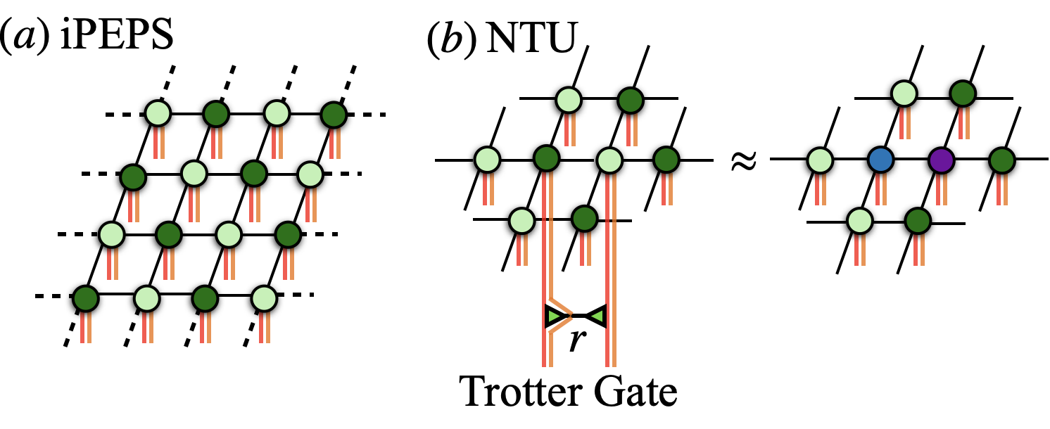
The imaginary time evolution of the purification, , is performed by the second-order Suzuki-Trotter decomposition of small time steps. An application of the NN two-site Trotter gate is outlined in Fig. 2(b) and in Appendix B. After a Trotter gate is applied to a bond connecting NN sites, its bond dimension is increased by a factor equal to the singular value decomposition (SVD) rank of the gate, . In order to prevent its exponential growth, the dimension is truncated with NTU to its original value, , in a way that minimizes the truncation error. NTU [105, 108] can be regarded as a special case of a cluster update [109, 110, 111], where the number of neighboring lattice sites taken into account during truncation makes for a refining parameter. The cluster update interpolates between a local truncation—as in the simple update (SU)—and the full update (FU) that takes into account all correlations in the truncated state [82]. As the NTU cluster includes the neighboring sites only, see Fig. 2(b), the NTU error can be calculated numerically exactly via parallelizable tensor contractions [105, 108]. We provide short description of the algorithm in Appendix B. That exactness warrants that the error measure is Hermitian and non-negative down to the numerical precision, unlike in the case of FU that involves the approximate corner transfer matrix renormalization group (CTMRG) [112, 113, 60, 114]. It is thus an optimal trade-off for applications where quantum correlations are not too long like in, e.g., Kibble-Zurek quenches in 2D [115] or time evolution of many-body localizing systems [108]. Therefore, it should perform well for the Hubbard model at intermediate and high temperatures, as we demonstrate in Appendix D using spinless non-interacting fermions and available DCA results for FHM [116]. We apply iPEPS with bond dimensions up to to the Hubbard model directly in the thermodynamic limit in a regime complementary to iPEPS simulations at zero temperature [117, 47], exponential thermal renormalization group (XTRG) of a small square lattice [95], or minimally entangled typical thermal states (METTS) on thin cylinders [48].
III Results
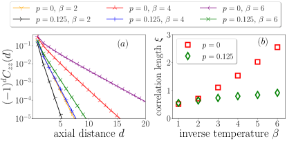
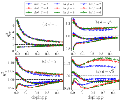
At half-filling and for large on-site Coulomb repulsion , FHM can be mapped to the Heisenberg model. The Heisenberg model develops long-range AFM order at zero temperature and strong correlations persist even at moderate temperatures [118]. In case of FHM, these AFM correlations do not perish even at low doping for low and intermediate temperatures [119]. We corroborate these findings with our iPEPS simulations by calculating two-site spin-spin correlation function along the -direction: , where and is the distance along axial direction. In Fig. 3(a), we plot the correlators for half-filling (), and at .
In Fig. 3(b), we plot the -dependence of the axial correlation length , characterizing , extracted from a transfer matrix (see Appendix D for details). that we reach for would be problematic on a thin cylinder or in a small system. The length is shorter for doping where doping undermines the AFM order. We verified the convergence of the results with the bond dimension of PEPS tensors.
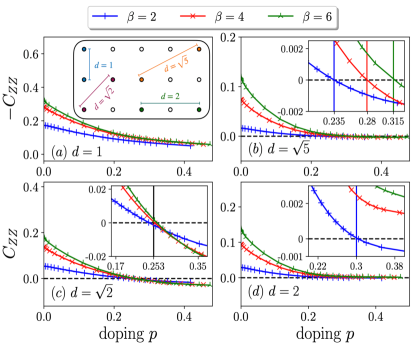
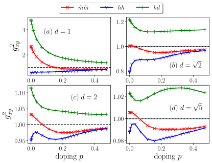
In Fig. 4 we present several short-range correlators: (nearest axial correlator), (nearest diagonal correlator), (next nearest axial correlator), and (next nearest diagonal correlator) in the function of a doping. It is motivated by a recent experiment [35] in a small system of ultra-cold atoms, where a change of sign in has been observed around doping , that is not inconsistent with numerical XTRG study of small lattices up to sites [95]. Our thermodynamic limit results in Fig. 4 further validate this effect. We also observe monotonic decreasing of the correlator with doping with no characteristic minima seen in the finite-system data. It has been long noted that a hole traveling through a strongly-coupled Hubbard model near the half-filling leaves behind a trail of ferromagnetically ordered regions in the AFM background [120, 121, 122, 123], as illustrated in Fig. 1. One expects that the magnitude of two-point correlators decreases with increasing doping since the interaction between holes and the AFM background creates magnetic polarons. This phenomenon is captured particularly well through the sign reversal in diagonal correlators and has been argued [35] to be explained by the geometric string theory [36]. We recover this feature in our simulations in Fig. 4(b), where we observe a change of sign around for all three inverse temperatures, .
Other correlators, and , show qualitative similarity with those obtained in [95], albeit without suffering from finite-size effects. Furthermore, we obtain longer-range correlators like, e.g., the second diagonal correlator . It undergoes a similar change of sign at for all three temperatures providing another strong validation of the string theory [35]. We obtain converged values of doping (where the sign changes) by working in the thermodynamic limit with iPEPS. It could potentially help benchmark other numerical methods and experiments. Note that due to finite size effects, previous approaches have been unable to obtain sharp estimates for this sign reversal.
Important characteristics of the doped FHM can also be revealed by charge correlators. The interesting two-point charge correlators usually considered are the hole-hole, , correlator where hole and hole-doublon correlator, , where . The quantum gas microscopy techniques overestimate and cannot distinguish between holes and doublons, as they both appear the same after imaging, but it can instead measure anti-moment correlators, , of . Nevertheless, recent developments promise hole-doublon correlators measurements in the near-future [124]. First, we calculate normalized hole-hole , hole-doublon , and anti-moment correlation functions at inverse temperature :
| (2) |
plotting the results in Fig. 5. We find that both and show strong bunching near half filling (), indicating the presence of nearest neighbor hole-doublon pairs. This is further supported by the fact that beyond , both and show much weaker bunching effect. At high doping, anti-bunching effects from hole-hole correlators dominate and contribute to the cross-over of correlators from bunching to anti-bunching. The behaviour of the correlators at , and remains qualitatively similar to the ones at , though much less pronounced. Our results are qualitatively consistent with finite-size experiments [36, 24, 35, 124] and numerics [95].
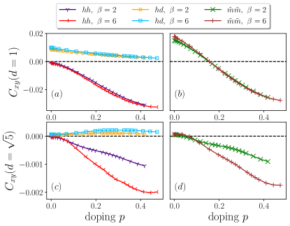
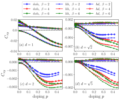
Next, in Fig. 6, we show connected hole-hole , hole-doublon and anti-moment correlation functions for axial nearest neighbor () and next nearest diagonal ():
| (3) |
We do not plot the doublon-doublon correlators as their magnitude is relatively small, , for NN correlators. It is important to note that, as , it is primarily the competition between and that drives the magnitude of . We see in Fig. 6 that as the system is gradually doped away from half-filling, the hole-doublon correlations decrease in magnitude while the hole-hole correlations increase significantly. Interestingly, shows strong dependence on temperature beyond , see Fig. 6(c). For additional data on correlators, see the Appendix E.
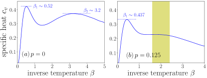
Finally, in Fig. 7, we show specific heat as a function of the inverse temperature. We tune different chemical potentials to achieve desired doping of at each temperature point. We develop a method to control particle density by interpolating the chemical potential during imaginary-time simulation, see App. F for details. In practice, however, we did not end up using it, as NTU evolution with different chemical potentials, avoiding computationally expensive CTMRG, can be executed more efficiently. The energy per site used here reads
| (4) |
where runs over NN sites of the site . Motivated by high-temperature expansion, numerical data for were fitted with a polynomial in to stabilise numerical derivative. With increasing degree of the polynomial, but still far from overfitting, the specific heat converges to a curve with two peaks. For , there is a sharp peak at and a broad one around . The former, known as the charge peak, is related to the suppression of the double occupancy. The latter is located near a point, which in the case of half-filling, corresponds to the crossover from a spin-disordered paramagnet to a state with NN antiferromagnetic correlations. It is known as the spin peak. As the doping undermines the AFM order this crossover is less pronounced at . Our results are in qualitative agreement with the quantum Monte Carlo on a cluster [125] but they are free from finite-size effects.
IV Conclusion
We extend the NTU algorithm to study spinful fermionic systems. We employ it to the challenging FHM in the 2D square infinite lattice at a finite temperature. We calculate expectation values for a set of observables that could be probed directly in prospective ultracold atoms experiments. By eliminating finite-size effects, we make contact with the current technology where large samples of atoms in almost homogeneous box-like trapping potentials can be probed. We cover a range of temperatures and dopings, including those accessible to the current experiments.
Acknowledgements.
AS is indebted to Gabriela Wojtówicz, Titas Chanda and Juraj Hasik for useful discussions. We also thank Juraj Hasik and Krzysztof Wohlfeld for useful comments on the manuscript. PC acknowledges initial support from Laboratory Directed Research and Development (LDRD) program of Los Alamos National Laboratory (LANL) under project number 20190659PRD4 with subsequent support by by the National Science Centre (NCN), Poland under project 2019/35/B/ST3/01028. This research was supported in part by the National Science Centre (NCN), Poland under projects 2019/35/B/ST3/01028 (AS, JD) and 2020/38/E/ST3/00150 (MR).Appendix A iPEPS and symmetries
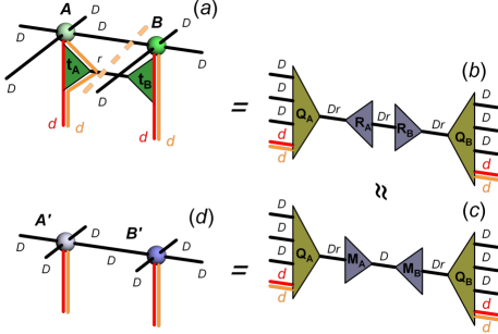
The iPEPS ansatz used in this work assumes a checkerboard lattice of tensors with two sites, and , in a unit cell. We depict it in Fig. A1(a). Each iPEPS tensor has four legs containing virtual degrees of freedom—each with total bond dimension , a physical index , and an ancillary index . The imaginary-time-evolved iPEPS , which represents a purification of the thermal density operator , is obtained by an action of an evolution operator on an uncorrelated product state at infinite temperature . We choose the initial state to be a product of maximally entangled states of every physical site with its ancilla: , where enumerates the lattice sites and refers to spin degrees of freedom—with two spin species at each lattice site for FHM. The density operator results from tracing out the ancillary degrees of freedom of the purification
The FHM Hamiltonian preserves numbers of electrons with spins and . Therefore, is invariant under a symmetry transformation ,
| (A2) |
where is a product over all lattice sites, is a unitary matrix representation of group with , where is a particle number operator with spin on site , and .
To enforce this abelian symmetry, an iPEPS representing is constructed from invariant tensors [126, 127],
| (A3) |
and analogously for . Here, , , and are unitary matrix representations acting at virtual indices of the iPEPS tensor , and and , respectively, label physical and ancillary degrees of freedom of a lattice site. It can now be decomposed into symmetric sectors labeled by charges corresponding to each index of [126],
| (A4) |
Dimensions of virtual indices of the sectors are called sectorial bond dimensions .
In the case of , the charges are formed by pairs of integers, . To ensure invariance of and , they obey
| (A5) |
where the signs (or signatures) correspond to hermitian conjugations in Eq. (A3). For non-interacting spinless fermions discussed in App. D, we have preservation of the total number of fermions manifesting itself as symmetry of iPEPS tensors. In such a case , where is a fermion density operator at site and the charges are integers summing up to zero as in Eq. (A5).
The symmetries are implemented with YAST symmetric tensor library [128] that we employ in this work. They are instrumental not only to obtain sparser tensors, allowing to reach significantly larger bond dimensions , but also to enforce fermionic statistics. For the latter, we follow a general scheme of Refs. [106, 107].
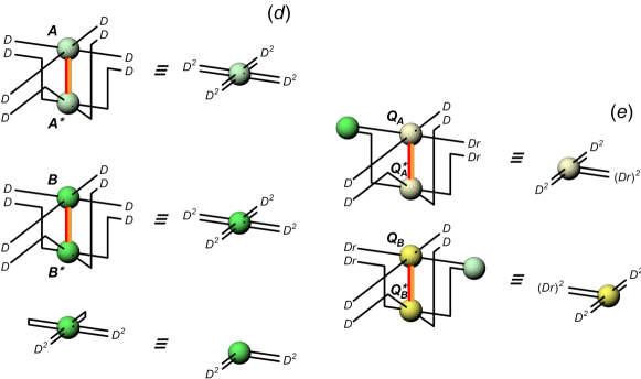
Enforcing fermionic statistics amounts to projecting the tensor network on a plain where the line crossings indicate the application of a SWAP gate. This requires symmetric tensors with fermionic parity defined for each tensor leg. In our case, the fermionic parity equals parity of . A SWAP gate applied to two tensor legs multiplies by all tensor blocks (defined in Eq. (A4) for a particular tensor with 6 legs) that have odd fermionic parity on both those legs. In particular, such leg crossings appear in Figs. A1, A2, and A3. These figures are the building blocks of the NTU algorithm described in the next section.
All expectation values in this work are calculated using the standard corner transfer matrix renormalization group (CTMRG) [113, 60, 114] and have been converged against environmental bond dimension which is its refinement parameter. CTMRG is also used to estimate the largest correlation length in the system using the largest eigenvalues of CTMRG row-to-row and column-to-column transfer matrices [129]. We ensured that they have been converged against as well.
Appendix B NTU evolution algorithm
The time-evolution method is explained in some detail by the diagrams in Figs. A1, A2, A3, and A4. The following text serves as a guide through the figures.
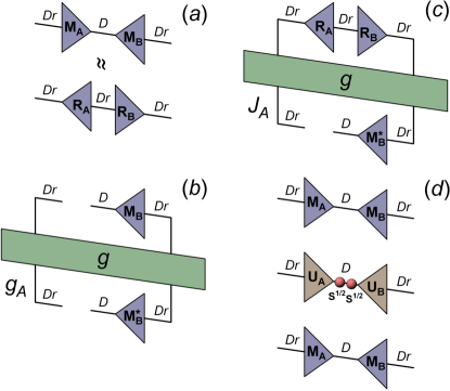
The evolution operator is applied to the tensors sequentially as a product of small time-steps , each of them approximated by a series of local gates via the second-order Suzuki-Trotter decomposition. Fig. A2(a) shows in detail the gate applied to a horizontal pair of nearest-neighbor iPEPS tensors, and , the same as in Fig. A1(b). The rank- gate enlarges the bond dimension from to , that will be truncated back to . For better numerical efficiency, we use QR decomposition to compute reduced matrices and in place of full tensors [130], see Fig. A2(b). Their product, , is to be approximated by a product of new matrices contracted through a bond of dimension : , see Fig. A2(c). Those matrices get combined with isometries and into the new iPEPS tensors and in Fig. A2(d). However, before this final contraction, the matrices are subject to NTU optimization.
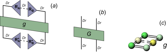
The NTU optimization of the reduced matrices and minimizes the Frobenius norm of the difference between the two sides of the equation in Fig. A1(b). As the diagrams in Figs. A2(c) and (d) are equal, the RHS of the equation in Fig. A1(b) is linear in product , and the norm squared of the difference between the LHS and the RHS can be written as
| (B6) |
where is a metric tensor defined by this construction. The tensor can be directly computed as in Fig. A3. Thanks to its numerical exactness, is a manifestly non-negative and Hermitian matrix. Matrices and are optimized to minimize the cost function (B6) or, equivalently, to make their product, , the best approximation to the exact product, . Their optimization proceeds iteratively:
| (B7) |
until convergence of the cost function.
When optimizing for fixed , the cost function (B6) becomes quadratic in :
| (B8) |
Here and depend on , see Figs. A4(b) and (c), and -independent is shown in Fig. A3(a). The matrix is updated as
| (B9) |
where the tolerance of the pseudo-inverse is dynamically adjusted to minimize . Thanks to the exactness of , the reduced is also a manifestly non-negative and Hermitian matrix. As there is no need to correct exact , the only role of the dynamical tolerance is to keep the influence of numerical inversion errors under control. In practice, the optimal tolerance remains in the range — relative to the maximal eigenvalue of . The numerical exactness of and its practical consequences provide key motivation behind the NTU scheme.
The optimization of is followed by a similar optimization of . The two optimizations are repeated until convergence of a relative NTU error:
| (B10) |
This error measures the accuracy of the NTU tensor truncation. The square root makes an estimate for a relative error of the purification inflicted by the truncation after the Trotter gate and thus also of errors of its expectation values. Therefore, for a small enough imaginary time-step, it should become proportional to making a step-size-independent measure of the error caused by the truncation.
The truncation errors accumulate with evolution time. As long as the errors remain small, the worst case scenario is that they are additive. The additiveness should hold at least over short time intervals over which the purification does not change much, and small errors made by subsequent truncations point in approximately the same direction in the Hilbert space. This heuristic reasoning motivates an integrated NTU error:
| (B11) |
where the sum is over all Trotter gates between and , as a relevant estimate of the purification error at . We employ this estimate in the main text.
Appendix C Initialization of updated tensors
In this section, we elaborate on the initialization of matrices and , see Fig. A2(b) and (c). As already indicated in the figure caption, a traditional strategy, practiced in full update, see [131] for an introductory review, is to make an SVD decomposition of the product before truncating it to dominant singular values.
The state-of-the-art SVD initialization, however, knows nothing about the tensor environment of the product. With poor initialization, the iteration procedure of Eq. (B7) may end up getting trapped in a local minimum. More importantly, for the symmetric iPEPS, the total bond dimension is a sum of sectorial bond dimensions . The iterative NTU optimization (B7) is working within a fixed distribution of , not being able to update it even though it takes into account the NTU environment exactly. This might lead to misrepresentation of the evolved state and makes proper initialization of truncated matrices and , with a particular distribution of , a crucial part of a successful algorithm. Below, we discuss two methods that we employ in this work.
C.1 Environment-assisted truncation
In order to take into account the environment in an approximate way, we propose the environment-assisted truncation (EAT). While here the environment taken into account is the NTU cluster in Fig. A1(b), the scheme can be directly employed in larger or infinite environments.
The norm squared of the product is shown in Fig. A3(a), where the metric tensor encapsulates relevant information about the NTU environment. Cutting the dashed bonds in Fig. A3(a) creates metric tensor in Fig. A3(b). By construction, within the NTU scheme, it is manifestly Hermitian and non-negative. If an object were inserted in the dashed bonds then would measure its norm. If the object were a projector truncating the bond dimension then would measure the error of the truncation.
EAT approximates in Fig. A3(b) with a product of metric tensors, , see Fig. A5. The approximation is done by an SVD of between its left and right indices, truncated to the dominant singular value. After eventual adjustment of phases of the leading left and right singular vectors, both and are manifestly Hermitian and non-negative. This property is inherited from the NTU metric . The advantage of the product is that – while it does not ignore the tensor environment – reduced matrices and can still be initialized using a simple SVD, see Fig. A5(b). Similarly as after the traditional SVD initialization, the initial matrices and are further optimized to minimize the NTU error in the exact NTU environment.
Before we proceed, to put it into broader context, it is worth considering the application of EAT in a one-dimensional setup of matrix product states. In that case, the rank-1 approximation of the metric tensor performed in Fig. A5(a) would be exact, with and being the exact left and right environments of a given bond. The following steps in Fig. A5 amount in that case to the optimal truncation of that bond [132], without the need for further iterative updates. This is not the case for a 2D setup, where EAT in A5(a) takes the first product approximation of the environment, but still going beyond the standard SVD initialization that does not input any information about the environment.
| {} | |
|---|---|
| 14 | (0,0):2, (-1,0):2, (1,0):2, (0,-1):2, (0,1):2, (-1,-1):1, (-1,1):1, (1,-1):1, (1,1):1 |
| 15 | (0,0):3, (-1,0):2, (1,0):2, (0,-1):2, (0,1):2, (-1,-1):1, (-1,1):1, (1,-1):1, (1,1):1 |
| 16 | (0,0):4, (-1,0):2, (1,0):2, (0,-1):2, (0,1):2, (-1,-1):1, (-1,1):1, (1,-1):1, (1,1):1 |
| 20 | (0,0):4, (-1,0):2, (1,0):2, (0,-1):2, (0,1):2, (-1,-1):2, (-1,1):2, (1,-1):2, (1,1):2 |
| 24 | (0,0):4, (-1,0):3, (1,0):3, (0,-1):3, (0,1):3, (-1,-1):2, (-1,1):2, (1,-1):2, (1,1):2 |
| 25 | (0,0):5, (-1,0):3, (1,0):3, (0,-1):3, (0,1):3, (-1,-1):2, (-1,1):2, (1,-1):2, (1,1):2 |
| 26 | (0,0):6, (-1,0):3, (1,0):3, (0,-1):3, (0,1):3, (-1,-1):2, (-1,1):2, (1,-1):2, (1,1):2 |
| 29 | (0,0):5, (-1,0):4, (1,0):4, (0,-1):4, (0,1):4, (-1,-1):2, (-1,1):2, (1,-1):2, (1,1):2 |
| {} | |
|---|---|
| 7 | -1:2, 0:3, 1:2 |
| 9 | -2:1, -1:2, 0:3, 1:2, 2:1 |
| 10 | -2:1, -1:2, 0:4, 1:2, 2:1 |
| 11 | -2:1, -1:2, 0:5, 1:2, 2:1 |
| 14 | -2:1, -1:4, 0:4, 1:4, 2:1 |
| 16 | -2:1, -1:3, 0:8, 1:3, 2:1 |
| 19 | -2:2, -1:4, 0:7, 1:4, 2:2 |
| 25 | -2:2, -1:6, 0:9, 1:6, 2:2 |
One may now consider options to further improve the initialization procedure. One such option is to perform a gradual truncation within a -step EAT+NTU (EATm). In this procedure the initial truncation is done not in one but in steps as , where is the SVD rank of the Trotter gate applied. For example, a 2-step EAT (EAT2) would involve truncating to, say, with EAT, followed by optimization with the NTU metric, and then subsequent truncation from to , ending with a final NTU optimization. During the first truncation metric is subject to the product approximation, , making the partial truncation of matrices and suboptimal. The following NTU optimization improves the matrices with respect to exact metric . This improvement is reflected in a new metric — constructed as in Figs. A3(a,b) but with the partly truncated and in place of the untruncated and — defining the error measure for the second truncation. Consequently, the 2-step EAT should be less affected by the product approximation and, in particular, provide better choice of sectorial bond dimensions than the 1-step EAT.
C.2 Fixed distribution
Another truncation strategy is to constrain by hand in a way that reflects the spatial symmetries of the problem. First, we choose the same set of charges and their respective bond dimensions for each virtual leg of the iPEPS tensors. Second, we assign to charges with opposite signs, like and , the same bond dimensions, guided by an intuition that a current of fermions along a bond should be zero. The same set of is used throughout the whole imaginary time evolution. We try different distributions obeying those constraints and accept the one that yields the minimal NTU error. We call this strategy FIX. We collect virtual leg charges and their respective bond dimensions found with FIX in Tab. A1. Results in the main text and following App. D have been obtained with the parameters listed in the tables.
Initialization of matrices and in each charge sector with predefined was performed with EAT. It gives a better initial NTU error, , than the SVD truncation and, therefore, should help to prevent the following NTU optimization of from getting trapped in a local minimum. For the half-filled Hubbard model we find that using FIX with EAT initialization typically results in the best NTU error while comparing to SVD and EAT schemes, see examples in Fig. A6. We note that for some , EAT or both SVD and EAT initialization give similar as FIX. This behavior is not unexpected as some optimization instances can be less affected by local minima than others. Consequently, we use FIX with EAT initialization (the combo being labelled as FIX for simplicity—which has negligible overhead over FIX with SVD initialization) for all the simulations in the main text and the following benchmarks in App. D.
We compare the final NTU errors for evolutions with the EAT initialization schemes and SVD scheme for the Hubbard model at half-filling using the NTU error . We see that in some cases both 1-step and 2-step EAT clearly outperforms the SVD initialization while in the others they gives results of similar quality, see examples in Fig. A6. In our simulations we find that a 2-step EAT (EAT2) procedure, in general, leads to slightly lower NTU error than the 1-step version (EAT1), and we use the former for our benchmarks in App. D. For simplicity, we henceforth label a 2-step EAT initialization procedure as EAT.
Appendix D Benchmarks
In order to demonstrate that our algorithm works properly, we collect a series of benchmark results. The evolution is performed in Trotter steps of size , which we found was small enough for step-size independence. The same time step was used for the results presented in the main text.
To begin with, we consider non-interacting spinless fermions for which we can compare with analytical results:
| (D12) |
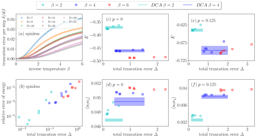
We pushed our simulations up to . Fig. A7(a) shows that, as expected, the NTU error (B10) during the evolution decreases with increasing total bond dimension. Fig. A7(b) shows the relative error of energy as a function of the integrated NTU error (B11), which in App. B was argued to be a useful measure of evolution error. Here we define the relative error as , where is the energy from our simulations and is the exact energy of the Fermi sea. We see a systematic trend where the energy error decreases with decreasing integrated NTU error . It demonstrates the usefulness of as an error estimator.
Next, we move on to the FHM, where we enforce average dopings of and fermion per site and consider the strongly interacting case of . In Fig. A7, we plot and compare the energy per site and double occupancy for and with the dynamical cluster approximation (DCA) results [116]. Our results are in good agreement with DCA. Additionally, we see similar quality of convergence for as for as a function of decreasing . This boosts confidence in our results for correlators obtained at in the main text. Here, we set to enforce , and to fix we scan and fine-tune different chemical potentials, see Tab. A2.
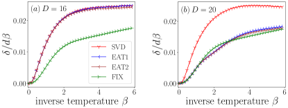
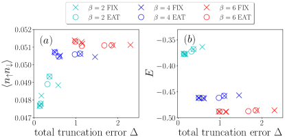
Finally, in Fig. A8 EAT yields comparable quality of results as FIX in the Hubbard model at half-filling, mutually corroborating both simulation strategies.
| 14 | -2.2 | -2.247 | -2.277 |
|---|---|---|---|
| 15 | -2.164 | -2.17 | -2.18 |
| 16 | -2.172 | -2.164 | -2.167 |
| 20 | -2.176 | -2.16 | -2.158 |
| 25 | -2.18 | -2.17 | -2.17 |
Appendix E Additional data for charge correlators
For interested readers, we provide additional results for charge correlators. In Fig. A9, we plot normalized hole-hole , hole-doublon , and anti-moment correlators for three values of inverse temperatures and (in the main text, we only provide the data for for clarity):
| (E13) |
In Fig. A10, we show connected correlators for the same observables:
| (E14) |
Interestingly, the longer the range of the two-point correlator, the stronger the temperature dependence, while for nearest neighbor correlators, , there is no discernible dependence on temperature, see Fig. A9(a) and Fig. A10(a). We use iPEPS bond dimension and environmental bond dimension for calculation of correlators. The parameters used were found to be sufficient to achieve convergence against bond dimension.
Appendix F Shifting the particle density
The purification obtained by imaginary time evolution in is—up to errors inflicted by the truncation of bond dimensions after every Trotter gate—equal to . The evolution is performed with a fixed chemical potential . The simulation can be repeated for different values of , but in general, it is not known beforehand what has to be adopted for a given to reach the desired doping, say, . One can bypass this problem by performing evolutions for a grid of and then “interpolating” to the that yields the desired particle density. At first sight, the interpolation is rather simple because the total particle number, , commutes with the Hamiltonian. Therefore, knowing for a given , we can obtain a purification for and the same simply by applying to the physical indices of the iPEPS. This transformation can be conveniently implemented by applying a local operator to the physical index of each purification tensor.
In practice, one has to be cautious because the purification, , is approximated by a tensor network whose bond dimension was truncated after each Trotter gate. The truncation was optimized to minimize the error for a given , but the same truncation may turn out not to be optimal for when gets too large. To be more specific, density operator has a particle number distribution, . It is reasonable to assume that for given and the truncations were optimized to minimize the error of the dominant central part of the distribution as the optimized cost function had little sensitivity to the errors of its tails, and the relative errors of the tails may remain large. After the transformation we obtain
| (F15) |
The exponential prefactor shifts the maximum of the new distribution comparing to the old one. When the new maximum is within the error-afflicted tail of the old distribution, the large prefactor magnifies the tail errors. The new distribution fails to be accurate in its new central part, though it remains unreasonably precise in the old central part, which is now an irrelevant tail. This happens when is too large.
What does it mean too large and how does acceptable depend on ? We expect that for sufficiently large , the distribution localizes on the ground state, which has definite , and has very small variance in this regime. Therefore, at sufficiently low temperatures, the allowed magnitude of decreases with increasing . The lower are the temperatures at which we want to target a predefined particle density, the finer must be a grid in the chemical potential on which we generate the -evolutions.
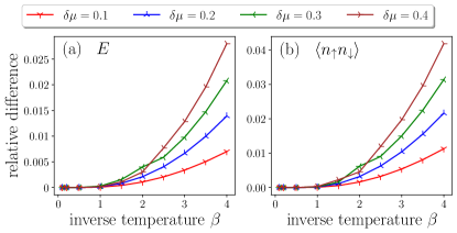
To see if the grid is fine enough, we can make cross-checks between and , where is the grid resolution, calculating an observable either directly in the purification at or in the purification at transformed back to . We corroborate the discussion in Fig. A11, where we plot the relative difference in observable, defined by , where is the expectation value calculated at a chemical potential and is the expectation value shifted from to . Qualitatively the differences depend on and as predicted, adding confidence to the rationale behind the method. For , which is still quite large, the differences are small.
Since, in our simulations, the NTU evolution was much cheaper than the calculation of expectation values (that employs corner transfer matrix renormalization), we did not use the -interpolation. We could afford to generate a fine enough -grid to avoid unnecessary interpolation errors.
References
- Lieb and Wu [1968] E. H. Lieb and F. Y. Wu, Absence of Mott transition in an exact solution of the short-range, one-band model in one dimension, Phys. Rev. Lett. 20, 1445 (1968).
- Lieb and Wu [2003] E. H. Lieb and F. Wu, The one-dimensional Hubbard model: a reminiscence, Physica A 321, 1 (2003).
- Qin et al. [2022] M. Qin, T. Schäfer, S. Andergassen, P. Corboz, and E. Gull, The Hubbard model: A computational perspective, Annu. Rev. Condens. Matter Phys. 13, 275 (2022).
- Lewenstein et al. [2007] M. Lewenstein, A. Sanpera, V. Ahufinger, B. Damski, A. Sen(De), and U. Sen, Ultracold atomic gases in optical lattices: mimicking condensed matter physics and beyond, Adv. Phys. 56, 243 (2007).
- Bloch et al. [2008] I. Bloch, J. Dalibard, and W. Zwerger, Many-body physics with ultracold gases, Rev. Mod. Phys. 80, 885 (2008).
- Bloch et al. [2012] I. Bloch, J. Dalibard, and S. Nascimbene, Quantum simulations with ultracold quantum gases, Nat. Phys. 8, 267 (2012).
- Strohmaier et al. [2007] N. Strohmaier, Y. Takasu, K. Günter, R. Jördens, M. Köhl, H. Moritz, and T. Esslinger, Interaction-controlled transport of an ultracold fermi gas, Phys. Rev. Lett. 99, 220601 (2007).
- Schneider et al. [2008] U. Schneider, L. Hackermüller, S. Will, T. Best, I. Bloch, T. A. Costi, R. W. Helmes, D. Rasch, and A. Rosch, Metallic and insulating phases of repulsively interacting fermions in a 3D optical lattice, Science 322, 1520 (2008).
- Jördens et al. [2008] R. Jördens, N. Strohmaier, K. Günter, H. Moritz, and T. Esslinger, A Mott insulator of fermionic atoms in an optical lattice, Nature 455, 204 (2008).
- Jördens et al. [2010] R. Jördens, L. Tarruell, D. Greif, T. Uehlinger, N. Strohmaier, H. Moritz, T. Esslinger, L. De Leo, C. Kollath, A. Georges, et al., Quantitative determination of temperature in the approach to magnetic order of ultracold fermions in an optical lattice, Phys. Rev. Lett. 104, 180401 (2010).
- Esslinger [2010] T. Esslinger, Fermi-Hubbard physics with atoms in an optical lattice, Annu. Rev. Condens. Matter Phys. 1, 129 (2010).
- Tarruell and Sanchez-Palencia [2018] L. Tarruell and L. Sanchez-Palencia, Quantum simulation of the Hubbard model with ultracold fermions in optical lattices, C. R. Phys. 19, 365 (2018).
- Hofstetter and Qin [2018] W. Hofstetter and T. Qin, Quantum simulation of strongly correlated condensed matter systems, J. Phys. B: At. Mol. Opt. 51, 082001 (2018).
- Bohrdt et al. [2021a] A. Bohrdt, L. Homeier, C. Reinmoser, E. Demler, and F. Grusdt, Exploration of doped quantum magnets with ultracold atoms, Annals of Physics 435, 168651 (2021a).
- Bakr et al. [2009] W. S. Bakr, J. I. Gillen, A. Peng, S. Fölling, and M. Greiner, A quantum gas microscope for detecting single atoms in a Hubbard-regime optical lattice, Nature 462 (2009).
- Sherson et al. [2010] J. F. Sherson, C. Weitenberg, M. Endres, M. Cheneau, I. Bloch, and S. Kuhr, Nature 467 (2010).
- Kuhr [2016] S. Kuhr, Quantum-gas microscopes: a new tool for cold-atom quantum simulators, Natl. Sci. Rev. 3, 170 (2016).
- Gross and Bakr [2021] C. Gross and W. S. Bakr, Quantum gas microscopy for single atom and spin detection, Nat. Phys. 17, 1316 (2021).
- Cheuk et al. [2015] L. W. Cheuk, M. A. Nichols, M. Okan, T. Gersdorf, V. V. Ramasesh, W. S. Bakr, T. Lompe, and M. W. Zwierlein, Quantum-gas microscope for fermionic atoms, Phys. Rev. Lett. 114, 193001 (2015).
- Haller et al. [2015] E. Haller, J. Hudson, A. Kelly, D. A. Cotta, B. Peaudecerf, G. D. Bruce, and S. Kuhr, Nat. Phys. 11 (2015).
- Parsons et al. [2015] M. F. Parsons, F. Huber, A. Mazurenko, C. S. Chiu, W. Setiawan, K. Wooley-Brown, S. Blatt, and M. Greiner, Site-resolved imaging of fermionic in an optical lattice, Phys. Rev. Lett. 114, 213002 (2015).
- Edge et al. [2015] G. J. A. Edge, R. Anderson, D. Jervis, D. C. McKay, R. Day, S. Trotzky, and J. H. Thywissen, Imaging and addressing of individual fermionic atoms in an optical lattice, Phys. Rev. A 92, 063406 (2015).
- Greif et al. [2016] D. Greif, M. F. Parsons, A. Mazurenko, C. S. Chiu, S. Blatt, F. Huber, G. Ji, and M. Greiner, Site-resolved imaging of a fermionic Mott insulator, Science 351, 953 (2016).
- Cheuk et al. [2016] L. W. Cheuk, M. A. Nichols, K. R. Lawrence, M. Okan, H. Zhang, and M. W. Zwierlein, Observation of 2D fermionic Mott insulators of with single-site resolution, Phys. Rev. Lett. 116, 235301 (2016).
- Parsons et al. [2016] M. F. Parsons, A. Mazurenko, C. S. Chiu, G. Ji, D. Greif, and M. Greiner, Site-resolved measurement of the spin-correlation function in the Fermi-Hubbard model, Science 353, 1253 (2016).
- Boll et al. [2016] M. Boll, T. A. Hilker, G. Salomon, A. Omran, J. Nespolo, L. Pollet, I. Bloch, and C. Gross, Spin- and density-resolved microscopy of antiferromagnetic correlations in Fermi-Hubbard chains, Science 353, 1257 (2016).
- Brown et al. [2017] P. T. Brown, D. Mitra, E. Guardado-Sanchez, P. Schauß, S. S. Kondov, E. Khatami, T. Paiva, N. Trivedi, D. A. Huse, and W. S. Bakr, Spin-imbalance in a 2D Fermi-Hubbard system, Science 357, 1385 (2017).
- Islam et al. [2015] R. Islam, R. Ma, P. M. Preiss, M. Eric Tai, A. Lukin, M. Rispoli, and M. Greiner, Measuring entanglement entropy in a quantum many-body system, Nature 528, 77 (2015).
- Kaufman et al. [2016] A. M. Kaufman, M. E. Tai, A. Lukin, M. Rispoli, R. Schittko, P. M. Preiss, and M. Greiner, Quantum thermalization through entanglement in an isolated many-body system, Science 353, 794 (2016).
- Lukin et al. [2019] A. Lukin, M. Rispoli, R. Schittko, M. E. Tai, A. M. Kaufman, S. Choi, V. Khemani, J. Léonard, and M. Greiner, Probing entanglement in a many-body-localized system, Science 364, 256 (2019).
- Rispoli et al. [2015] M. Rispoli, A. Lukin, R. Schittko, S. Kim, M. E. Tai, J. Léonard, and M. Greiner, Quantum critical behaviour at the many-body localization transition, Nature 573, 385 (2015).
- Hilker et al. [2017] T. A. Hilker, G. Salomon, F. Grusdt, A. Omran, M. Boll, E. Demler, I. Bloch, and C. Gross, Revealing hidden antiferromagnetic correlations in doped Hubbard chains via string correlators, Science 357, 484 (2017).
- Koepsell et al. [2019] J. Koepsell, J. Vijayan, P. Sompet, F. Grusdt, T. A. Hilker, E. Demler, G. Salomon, I. Bloch, and C. Gross, Imaging magnetic polarons in the doped Fermi-Hubbard model, Nature 572, 358 (2019).
- Salomon et al. [2019] G. Salomon, J. Koepsell, J. Vijayan, T. A. Hilker, J. Nespolo, L. Pollet, I. Bloch, and C. Gross, Direct observation of incommensurate magnetism in Hubbard chains, Nature 565, 56 (2019).
- Chiu et al. [2019] C. S. Chiu, G. Ji, A. Bohrdt, M. Xu, M. Knap, E. Demler, F. Grusdt, M. Greiner, and D. Greif, String patterns in the doped Hubbard model, Science 365, 251 (2019).
- Grusdt et al. [2018] F. Grusdt, M. Kánasz-Nagy, A. Bohrdt, C. S. Chiu, G. Ji, M. Greiner, D. Greif, and E. Demler, Parton theory of magnetic polarons: Mesonic resonances and signatures in dynamics, Phys. Rev. X 8, 011046 (2018).
- Grusdt et al. [2019] F. Grusdt, A. Bohrdt, and E. Demler, Microscopic spinon-chargon theory of magnetic polarons in the model, Phys. Rev. B 99, 224422 (2019).
- Blomquist and Carlström [2020] E. Blomquist and J. Carlström, Unbiased description of magnetic polarons in a Mott insulator, Commun. Phys. 3 (2020).
- Bohrdt et al. [2020] A. Bohrdt, F. Grusdt, and M. Knap, Dynamical formation of a magnetic polaron in a two-dimensional quantum antiferromagnet, New J. Phys. 22, 123023 (2020).
- Ji et al. [2021] G. Ji, M. Xu, L. H. Kendrick, C. S. Chiu, J. C. Brüggenjürgen, D. Greif, A. Bohrdt, F. Grusdt, E. Demler, M. Lebrat, and M. Greiner, Coupling a mobile hole to an antiferromagnetic spin background: Transient dynamics of a magnetic polaron, Phys. Rev. X 11, 021022 (2021).
- Bohrdt et al. [2021b] A. Bohrdt, Y. Wang, J. Koepsell, M. Kánasz-Nagy, E. Demler, and F. Grusdt, Dominant fifth-order correlations in doped quantum antiferromagnets, Phys. Rev. Lett. 126, 026401 (2021b).
- Nielsen et al. [2021] K. K. Nielsen, M. A. Bastarrachea-Magnani, T. Pohl, and G. M. Bruun, Spatial structure of magnetic polarons in strongly interacting antiferromagnets, Phys. Rev. B 104, 155136 (2021).
- Wrzosek and Wohlfeld [2021] P. Wrzosek and K. Wohlfeld, Hole in the two-dimensional Ising antiferromagnet: Origin of the incoherent spectrum, Phys. Rev. B 103, 035113 (2021).
- Chang-Yan and Tin-Lun [2022] W. Chang-Yan and H. Tin-Lun, Interference of holon strings in 2D Hubbard model, arXiv:2203.12722 (2022).
- Kale et al. [2022] A. Kale, J. H. Huhn, M. Xu, L. H. Kendrick, M. Lebrat, C. Chiu, G. Ji, F. Grusdt, A. Bohrdt, and M. Greiner, Schrieffer-Wolff transformations for experiments: Dynamically suppressing virtual doublon-hole excitations in a Fermi-Hubbard simulator, Phys. Rev. A 106, 012428 (2022).
- Chao et al. [1977] K. A. Chao, J. Spalek, and A. M. Oles, Kinetic exchange interaction in a narrow s-band, J. Phys. C: Solid State Phys. 10, L271 (1977).
- Zheng et al. [2017] B.-X. Zheng, C.-M. Chung, P. Corboz, G. Ehlers, M.-P. Qin, R. M. Noack, H. Shi, S. R. White, S. Zhang, and G. K.-L. Chan, Stripe order in the underdoped region of the two-dimensional Hubbard model, Science 358, 1155 (2017).
- Wietek et al. [2021] A. Wietek, Y.-Y. He, S. R. White, A. Georges, and E. M. Stoudenmire, Stripes, antiferromagnetism, and the pseudogap in the doped Hubbard model at finite temperature, Phys. Rev. X 11, 031007 (2021).
- Xiao et al. [2022] B. Xiao, Y.-Y. He, A. Georges, and S. Zhang, arXiv:2202.11741 (2022).
- Ponsioen et al. [2019] B. Ponsioen, S. S. Chung, and P. Corboz, Period 4 stripe in the extended two-dimensional Hubbard model, Phys. Rev. B 100, 195141 (2019).
- Huang et al. [2017] E. W. Huang, C. B. Mendl, S. Liu, S. Johnston, H.-C. Jiang, B. Moritz, and T. P. Devereaux, Numerical evidence of fluctuating stripes in the normal state of high-Tc cuprate superconductors, Science 358, 1161 (2017).
- Verstraete et al. [2008] F. Verstraete, V. Murg, and J. Cirac, Matrix product states, projected entangled pair states, and variational renormalization group methods for quantum spin systems, Adv. Phys. 57, 143 (2008).
- Orús [2014] R. Orús, A practical introduction to tensor networks: Matrix product states and projected entangled pair states, Ann. Phys. (Amsterdam) 349, 117 (2014).
- Nishio et al. [2004] Y. Nishio, N. Maeshima, A. Gendiar, and T. Nishino, Tensor product variational formulation for quantum systems, arXiv:cond-mat/0401115 (2004).
- Verstraete and Cirac [2004] F. Verstraete and J. I. Cirac, Renormalization algorithms for quantum-many body systems in two and higher dimensions, arXiv:cond-mat/0407066 (2004).
- Murg et al. [2007] V. Murg, F. Verstraete, and J. I. Cirac, Variational study of hard-core bosons in a two-dimensional optical lattice using projected entangled pair states, Phys. Rev. A 75, 033605 (2007).
- Jordan et al. [2008] J. Jordan, R. Orús, G. Vidal, F. Verstraete, and J. I. Cirac, Classical simulation of infinite-size quantum lattice systems in two spatial dimensions, Phys. Rev. Lett. 101, 250602 (2008).
- Jiang et al. [2008] H. C. Jiang, Z. Y. Weng, and T. Xiang, Accurate determination of tensor network state of quantum lattice models in two dimensions, Phys. Rev. Lett. 101, 090603 (2008).
- Gu et al. [2008] Z.-C. Gu, M. Levin, and X.-G. Wen, Tensor-entanglement renormalization group approach as a unified method for symmetry breaking and topological phase transitions, Phys. Rev. B 78, 205116 (2008).
- Orús and Vidal [2009] R. Orús and G. Vidal, Simulation of two-dimensional quantum systems on an infinite lattice revisited: Corner transfer matrix for tensor contraction, Phys. Rev. B 80, 094403 (2009).
- Matsuda et al. [2013] Y. H. Matsuda, N. Abe, S. Takeyama, H. Kageyama, P. Corboz, A. Honecker, S. R. Manmana, G. R. Foltin, K. P. Schmidt, and F. Mila, Magnetization of SrCu(BO) in ultrahigh magnetic fields up to 118 T, Phys. Rev. Lett. 111, 137204 (2013).
- Corboz and Mila [2014] P. Corboz and F. Mila, Crystals of bound states in the magnetization plateaus of the Shastry-Sutherland model, Phys. Rev. Lett. 112, 147203 (2014).
- Liao et al. [2017] H. J. Liao, Z. Y. Xie, J. Chen, Z. Y. Liu, H. D. Xie, R. Z. Huang, B. Normand, and T. Xiang, Gapless spin-liquid ground state in the Kagome antiferromagnet, Phys. Rev. Lett. 118, 137202 (2017).
- Mei et al. [2017] J.-W. Mei, J.-Y. Chen, H. He, and X.-G. Wen, Gapped spin liquid with topological order for the kagome Heisenberg model, Phys. Rev. B 95, 235107 (2017).
- Phien et al. [2015] H. N. Phien, J. A. Bengua, H. D. Tuan, P. Corboz, and R. Orús, Infinite projected entangled pair states algorithm improved: Fast full update and gauge fixing, Phys. Rev. B 92, 035142 (2015).
- Corboz [2016a] P. Corboz, Variational optimization with infinite projected entangled-pair states, Phys. Rev. B 94, 035133 (2016a).
- Vanderstraeten et al. [2016] L. Vanderstraeten, J. Haegeman, P. Corboz, and F. Verstraete, Gradient methods for variational optimization of projected entangled-pair states, Phys. Rev. B 94, 155123 (2016).
- Fishman et al. [2018] M. T. Fishman, L. Vanderstraeten, V. Zauner-Stauber, J. Haegeman, and F. Verstraete, Faster methods for contracting infinite two-dimensional tensor networks, Phys. Rev. B 98, 235148 (2018).
- Xie et al. [2017] Z. Y. Xie, H. J. Liao, R. Z. Huang, H. D. Xie, J. Chen, Z. Y. Liu, and T. Xiang, Optimized contraction scheme for tensor-network states, Phys. Rev. B 96, 045128 (2017).
- Corboz [2016b] P. Corboz, Improved energy extrapolation with infinite projected entangled-pair states applied to the two-dimensional Hubbard model, Phys. Rev. B 93, 045116 (2016b).
- Corboz et al. [2018] P. Corboz, P. Czarnik, G. Kapteijns, and L. Tagliacozzo, Finite correlation length scaling with infinite projected entangled-pair states, Phys. Rev. X 8, 031031 (2018).
- Rader and Läuchli [2018] M. Rader and A. M. Läuchli, Finite correlation length scaling in lorentz-invariant gapless ipeps wave functions, Phys. Rev. X 8, 031030 (2018).
- Rams et al. [2018] M. M. Rams, P. Czarnik, and L. Cincio, Precise extrapolation of the correlation function asymptotics in uniform tensor network states with application to the Bose-Hubbard and XXZ models, Phys. Rev. X 8, 041033 (2018).
- Czarnik et al. [2012] P. Czarnik, L. Cincio, and J. Dziarmaga, Projected entangled pair states at finite temperature: Imaginary time evolution with ancillas, Phys. Rev. B 86, 245101 (2012).
- Czarnik and Dziarmaga [2014] P. Czarnik and J. Dziarmaga, Fermionic projected entangled pair states at finite temperature, Phys. Rev. B 90, 035144 (2014).
- Czarnik and Dziarmaga [2015a] P. Czarnik and J. Dziarmaga, Projected entangled pair states at finite temperature: Iterative self-consistent bond renormalization for exact imaginary time evolution, Phys. Rev. B 92, 035120 (2015a).
- Czarnik et al. [2016a] P. Czarnik, J. Dziarmaga, and A. M. Oleś, Variational tensor network renormalization in imaginary time: Two-dimensional quantum compass model at finite temperature, Phys. Rev. B 93, 184410 (2016a).
- Czarnik and Dziarmaga [2015b] P. Czarnik and J. Dziarmaga, Variational approach to projected entangled pair states at finite temperature, Phys. Rev. B 92, 035152 (2015b).
- Czarnik et al. [2016b] P. Czarnik, M. M. Rams, and J. Dziarmaga, Variational tensor network renormalization in imaginary time: Benchmark results in the Hubbard model at finite temperature, Phys. Rev. B 94, 235142 (2016b).
- Czarnik et al. [2017] P. Czarnik, J. Dziarmaga, and A. M. Oleś, Overcoming the sign problem at finite temperature: Quantum tensor network for the orbital model on an infinite square lattice, Phys. Rev. B 96, 014420 (2017).
- Dai et al. [2017] Y.-W. Dai, Q.-Q. Shi, S. Y. Cho, M. T. Batchelor, and H.-Q. Zhou, Finite-temperature fidelity and von Neumann entropy in the honeycomb spin lattice with quantum Ising interaction, Phys. Rev. B 95, 214409 (2017).
- Czarnik et al. [2019a] P. Czarnik, J. Dziarmaga, and P. Corboz, Time evolution of an infinite projected entangled pair state: An efficient algorithm, Phys. Rev. B 99, 035115 (2019a).
- Czarnik and Corboz [2019] P. Czarnik and P. Corboz, Finite correlation length scaling with infinite projected entangled pair states at finite temperature, Phys. Rev. B 99, 245107 (2019).
- Kshetrimayum et al. [2019] A. Kshetrimayum, M. Rizzi, J. Eisert, and R. Orús, Tensor network annealing algorithm for two-dimensional thermal states, Phys. Rev. Lett. 122, 070502 (2019).
- Czarnik et al. [2019b] P. Czarnik, A. Francuz, and J. Dziarmaga, Tensor network simulation of the Kitaev-Heisenberg model at finite temperature, Phys. Rev. B 100, 165147 (2019b).
- Jiménez et al. [2021] J. L. Jiménez, S. P. G. Crone, E. Fogh, M. E. Zayed, R. Lortz, E. Pomjakushina, K. Conder, A. M. Läuchli, L. Weber, S. Wessel, A. Honecker, B. Normand, C. Rüegg, P. Corboz, H. M. Rønnow, and F. Mila, A quantum magnetic analogue to the critical point of water, Nature 592, 370 (2021).
- Czarnik et al. [2021] P. Czarnik, M. M. Rams, P. Corboz, and J. Dziarmaga, Tensor network study of the magnetization plateau in the shastry-sutherland model at finite temperature, Phys. Rev. B 103, 075113 (2021).
- Poilblanc et al. [2021] D. Poilblanc, M. Mambrini, and F. Alet, Finite-temperature symmetric tensor network for spin-1/2 Heisenberg antiferromagnets on the square lattice, SciPost Phys. 10, 19 (2021).
- Vlaar and Corboz [2021] P. C. G. Vlaar and P. Corboz, Simulation of three-dimensional quantum systems with projected entangled-pair states, Phys. Rev. B 103, 205137 (2021).
- Cincio and Vidal [2013] L. Cincio and G. Vidal, Characterizing topological order by studying the ground states on an infinite cylinder, Phys. Rev. Lett. 110, 067208 (2013).
- Bruognolo et al. [2017] B. Bruognolo, Z. Zhu, S. R. White, and E. M. Stoudenmire, Matrix product state techniques for two-dimensional systems at finite temperature, arXiv:1705.05578 (2017).
- Chen et al. [2018a] B.-B. Chen, L. Chen, Z. Chen, W. Li, and A. Weichselbaum, Exponential thermal tensor network approach for quantum lattice models, Phys. Rev. X 8, 031082 (2018a).
- Chen et al. [2019] L. Chen, D.-W. Qu, H. Li, B.-B. Chen, S.-S. Gong, J. von Delft, A. Weichselbaum, and W. Li, Two-temperature scales in the triangular-lattice Heisenberg antiferromagnet, Phys. Rev. B 99, 140404(R) (2019).
- Li et al. [2019] H. Li, B.-B. Chen, Z. Chen, J. von Delft, A. Weichselbaum, and W. Li, Thermal tensor renormalization group simulations of square-lattice quantum spin models, Phys. Rev. B 100, 045110 (2019).
- Chen et al. [2021] B.-B. Chen, C. Chen, Z. Chen, J. Cui, Y. Zhai, A. Weichselbaum, J. von Delft, Z. Y. Meng, and W. Li, Quantum many-body simulations of the two-dimensional Fermi-Hubbard model in ultracold optical lattices, Phys. Rev. B 103, L041107 (2021).
- Abanin et al. [2016] D. A. Abanin, W. De Roeck, and F. Huveneers, Theory of many-body localization in periodically driven systems, Ann. Phys. (N. Y.) 372, 1 (2016).
- Li et al. [2011] W. Li, S.-J. Ran, S.-S. Gong, Y. Zhao, B. Xi, F. Ye, and G. Su, Linearized tensor renormalization group algorithm for the calculation of thermodynamic properties of quantum lattice models, Phys. Rev. Lett. 106, 127202 (2011).
- Xie et al. [2012] Z. Y. Xie, J. Chen, M. P. Qin, J. W. Zhu, L. P. Yang, and T. Xiang, Coarse-graining renormalization by higher-order singular value decomposition, Phys. Rev. B 86, 045139 (2012).
- Ran et al. [2012] S.-J. Ran, W. Li, B. Xi, Z. Zhang, and G. Su, Optimized decimation of tensor networks with super-orthogonalization for two-dimensional quantum lattice models, Phys. Rev. B 86, 134429 (2012).
- Ran et al. [2013] S.-J. Ran, B. Xi, T. Liu, and G. Su, Theory of network contractor dynamics for exploring thermodynamic properties of two-dimensional quantum lattice models, Phys. Rev. B 88, 064407 (2013).
- Ran et al. [2018] S.-J. Ran, W. Li, S.-S. Gong, A. Weichselbaum, J. von Delft, and G. Su, Emergent spin-1 trimerized valence bond crystal in the spin- Heisenberg model on the star lattice, Phys. Rev. B 97, 075146 (2018).
- Peng et al. [2017] C. Peng, S.-J. Ran, T. Liu, X. Chen, and G. Su, Fermionic algebraic quantum spin liquid in an octa-kagome frustrated antiferromagnet, Phys. Rev. B 95, 075140 (2017).
- Chen et al. [2018b] X. Chen, S.-J. Ran, T. Liu, C. Peng, Y.-Z. Huang, and G. Su, Thermodynamics of spin-1/2 Kagome Heisenberg antiferromagnet: algebraic paramagnetic liquid and finite-temperature phase diagram, Sci. Bull. 63, 1545 (2018b).
- Ran et al. [2019] S.-J. Ran, B. Xi, C. Peng, G. Su, and M. Lewenstein, Efficient quantum simulation for thermodynamics of infinite-size many-body systems in arbitrary dimensions, Phys. Rev. B 99, 205132 (2019).
- Dziarmaga [2021] J. Dziarmaga, Time evolution of an infinite projected entangled pair state: Neighborhood tensor update, Phys. Rev. B 104, 094411 (2021).
- Corboz and Vidal [2009] P. Corboz and G. Vidal, Fermionic multi-scale entanglement renormalization ansatz, Phys. Rev. B 80, 165129 (2009).
- Corboz et al. [2010] P. Corboz, R. Orús, B. Bauer, and G. Vidal, Simulation of strongly correlated fermions in two spatial dimensions with fermionic projected entangled-pair states, Phys. Rev. B 81, 165104 (2010).
- Dziarmaga [2022] J. Dziarmaga, Simulation of many-body localization and time crystals in two dimensions with the neighborhood tensor update, Phys. Rev. B 105, 054203 (2022).
- Wang and Verstraete [2011] L. Wang and F. Verstraete, Cluster update for tensor network states, arXiv:1110.4362 (2011).
- Lubasch et al. [2014a] M. Lubasch, J. I. Cirac, and M.-C. Bañuls, Unifying projected entangled pair state contractions, New J. Phys. 16, 033014 (2014a).
- Lubasch et al. [2014b] M. Lubasch, J. I. Cirac, and M.-C. Bañuls, Algorithms for finite projected entangled pair states, Phys. Rev. B 90, 064425 (2014b).
- Baxter [1978] R. J. Baxter, Variational approximations for square lattice models in statistical mechanics, J. Stat. Phys. 19, 461 (1978).
- Nishino and Okunishi [1996] T. Nishino and K. Okunishi, Corner Transfer Matrix Renormalization Group Method, J. Phys. Soc. Jpn. 65, 891 (1996).
- Corboz et al. [2014] P. Corboz, T. M. Rice, and M. Troyer, Competing states in the - model: Uniform -wave state versus stripe state, Phys. Rev. Lett. 113, 046402 (2014).
- Schmitt et al. [2022] M. Schmitt, M. M. Rams, J. Dziarmaga, M. Heyl, and W. H. Zurek, Quantum phase transition dynamics in the two-dimensional transverse-field Ising model, Sci. Adv. 8, eabl6850 (2022).
- LeBlanc et al. [2015] J. P. F. LeBlanc, A. E. Antipov, F. Becca, I. W. Bulik, G. K.-L. Chan, C.-M. Chung, Y. Deng, M. Ferrero, T. M. Henderson, C. A. Jiménez-Hoyos, et al., Solutions of the two-dimensional Hubbard model: Benchmarks and results from a wide range of numerical algorithms, Phys. Rev. X 5, 041041 (2015).
- Corboz et al. [2011] P. Corboz, S. R. White, G. Vidal, and M. Troyer, Stripes in the two-dimensional - model with infinite projected entangled-pair states, Phys. Rev. B 84, 041108(R) (2011).
- Manousakis [1991] E. Manousakis, The spin- Heisenberg antiferromagnet on a square lattice and its application to the cuprous oxides, Rev. Mod. Phys. 63, 1 (1991).
- Mazurenko et al. [2017] A. Mazurenko, C. S. Chiu, G. Ji, M. F. Parsons, M. Kanász-Nagy, R. Schmidt, F. Grusdt, E. Demler, D. Greif, and M. Greiner, A cold-atom Fermi-Hubbard antiferromagnet, Nature 545, 462 (2017).
- Nagaoka [1966] Y. Nagaoka, Ferromagnetism in a narrow, almost half-filled band, Phys. Rev. 147, 392 (1966).
- Nagaev [1968] E. Nagaev, Zh. Eksp. Teor. Fiz. 54, 228 (1968).
- Brinkman and Rice [1970] W. F. Brinkman and T. M. Rice, Single-particle excitations in magnetic insulators, Phys. Rev. B 2, 1324 (1970).
- Trugman [1988] S. A. Trugman, Interaction of holes in a Hubbard antiferromagnet and high-temperature superconductivity, Phys. Rev. B 37, 1597 (1988).
- Hartke et al. [2020] T. Hartke, B. Oreg, N. Jia, and M. Zwierlein, Doublon-hole correlations and fluctuation thermometry in a Fermi-Hubbard gas, Phys. Rev. Lett. 125, 113601 (2020).
- Duffy and Moreo [1997] D. Duffy and A. Moreo, Specific heat of the two-dimensional Hubbard model, Phys. Rev. B 55, 12918 (1997).
- Singh et al. [2011] S. Singh, R. N. C. Pfeifer, and G. Vidal, Tensor network states and algorithms in the presence of a global U(1) symmetry, Phys. Rev. B 83, 115125 (2011).
- Bauer et al. [2011] B. Bauer, P. Corboz, R. Orús, and M. Troyer, Implementing global abelian symmetries in projected entangled-pair state algorithms, Phys. Rev. B 83, 125106 (2011).
- [128] M. M. Rams, G. Wójtowicz, and J. Hasik, YAST – Yet Another Symmetric Tensor, https://gitlab.com/marekrams/yast .
- Nishino et al. [1996] T. Nishino, K. Okunishi, and M. Kikuchi, Numerical renormalization group at criticality, Phys. Lett. A 213, 69 (1996).
- Evenbly [2018] G. Evenbly, Gauge fixing, canonical forms, and optimal truncations in tensor networks with closed loops, Phys. Rev. B 98, 085155 (2018).
- Bruognolo et al. [2021] B. Bruognolo, J.-W. Li, J. von Delft, and A. Weichselbaum, A beginner’s guide to non-abelian iPEPS for correlated fermions, SciPost Physics Lecture Notes , 025 (2021).
- Orús and Vidal [2008] R. Orús and G. Vidal, Infinite time-evolving block decimation algorithm beyond unitary evolution, Phys. Rev. B 78, 155117 (2008).