Fermi motion effects in electroproduction of hypernuclei

Abstract

In a previous analysis of electroproduction of hypernuclei the cross sections were calculated using the distorted-wave impulse approximation where the momentum of the initial proton in the nucleus was set to zero (the “frozen-proton” approximation). In this paper we go beyond this approximation assuming a non zero effective proton momentum due to proton Fermi motion inside the target nucleus discussing also other kinematical effects. To this end we have derived a more general form of the two-component elementary electroproduction amplitude (Chew-Goldberger-Low-Nambu like) which allows its use in a general reference frame moving with respect to the nucleus rest frame. The effects of Fermi motion were found to depend on kinematics and elementary amplitudes. The largest effects were observed in the contributions from the longitudinal and interference parts of the cross sections. The extension of the calculations beyond the frozen-proton approximation improved the agreement of predicted theoretical cross sections with experimental data, and, once we assumed the optimum on-shell approximation, we were able to remove an inconsistency which was previously present in the calculations.

I Introduction

Studying the production of $\Lambda$ hypernuclei provides important information on details of the $\Lambda$N interaction, particularly on its spin-dependent part that is difficult to investigate in free $\Lambda$N scattering rijken99 . In fact, the effective $\Lambda$N interaction can be determined from hypernuclear spectra obtained from various reactions induced by hadron (mainly $\pi^{+}$ and $K^{-}$) and electron beams GHM2016 . Moreover, precise measurements of the production cross sections provide information on the hypernuclear production mechanism and the dynamics of the elementary production reaction. Whereas $\gamma$-ray hypernuclear spectra are measured with very high precision (a few keV), the spectra of (e, e^′ K⁺) reactions from nuclei are obtained only with resolution of several hundreds of keV, which is better than in the hadron-induced reactions hashtam06 but which still makes studying the fine splitting within the multiplets problematic. On the other hand, the reaction spectroscopy allows one to study also higher energy excited states, e.g., even between the nucleon emission threshold and the $\Lambda$ emission threshold which is not possible in $\gamma$-ray spectroscopy.

The electroproduction of strangeness is characterized by a large three-momentum transfer to the $\Lambda$ ($\approx$250 MeV/c), large angular momentum transfer $J$, and strong spin-flip terms, even at almost zero production angles hashtam06 . The latter results in the dominance of the highest-spin states in the multiplets. Moreover, the kaon production occurs on a proton in contrast to a neutron in the (K^-, $\pi^{-}$) and ($\pi^{+}$, K⁺) reactions allowing one to study different hypernuclei and charge-dependent effects from a comparison of mirror hypernuclei (Charge Symmetry Breaking). An important merit of electroproduction in view of its theoretical description is that the electro-magnetic part of the interaction is well known. A systematic experimental study of high-resolution hypernuclear spectroscopy in (e, e^′ K⁺) has been performed in Halls A archival and C HallC at Jefferson Laboratory (JLab). However, a reliable analysis of these data requires good understanding of the dynamics of the process and uncertainties arising from various approximations in a model.

Theoretical calculations of the cross sections in photo- and electroproduction of hypernuclei Cotanch ; Bennhold ; SF1994 ; HLee ; Lenske ; PTP2010 ; NPA2012 ; Motoba ; AIP2018 have been performed in the distorted-wave impulse approximation (DWIA) mainly assuming that the initial proton is at rest with respect to the nucleus. This “frozen-proton” approximation made it possible to use the nonrelativistic two-component Chew-Goldberger-Low-Nambu (CGLN) form of the elementary-production amplitude in the proton laboratory frame SF1994 , which significantly simplifies the calculations. However, as the proton is moving inside of the nucleus with a momentum about 150 MeV/c (in ¹²C), which is comparable to a momentum transfer of about 250 MeV/c, it is advisable to estimate effects arising from this proton Fermi motion. Note that to this end, in the approaches with a non relativistic shell-model description of the nuclear structure, one needs to derive the two-component form of the elementary electroproduction amplitude for a moving proton, i.e., the CGLN-like form in a general Lorentz frame moving with respect to the target-nucleus center of gravity.

The Fermi motion was included, e.g., in the elastic scattering of protons FM-proton and pions FM-pion from nuclei, via full folding (Fermi averaging) in the first-order optical potential. Note that here one needs an off-energy-shell extension of the elementary amplitude which introduces additional uncertainty in the calculation. Fermi motion effects were found to be important in calculating the cross sections in pion photoproduction off ¹⁰B Sato . On the other hand, in the DWIA analysis of the (K^-, $\pi^{-}$) reaction on ¹²C Zofka it was shown that accounting for the Fermi motion results only in a few percent reduction of the cross sections for hypernuclear production. The effects from motion of the target nucleon were also included in the DWIA calculations of the cross section in the ($\pi^{+}$, K⁺) and (K^-, $\pi^{-}$) reactions on the ¹²C target assuming optimal Fermi averaging of the on-shell elementary amplitude Harada . This averaging of the amplitude leads to improvement in the data description. A Fermi averaged amplitude was also used in the study of formation of p-shell hypernuclei in the (K^-, $\pi^{-}$) reactions Auerbach . Nonlocalities in photoproduction of hypernuclei arising from Fermi motion were included in Refs. Bennhold ; Lenske using relativistic nuclear models. These effects were found to make changes of about 20% (and more) in the cross sections for the high-spin transitions which dominate in a multiplet Bennhold .

In this paper we study effects of Fermi motion of the initial proton in DWIA calculations of the cross sections in ¹²C(e,e^′K⁺)${}^{12}_{~{}\Lambda}$B. In order to avoid uncertainties related to an off-energy-shell extension of the elementary amplitude, constructed for production on a free proton SB18 ; SLA , the amplitude is considered on-shell in the optimal factorisation approximation. This approach was already used in our previous calculations NPA2012 ; archival ; AIP2018 and here we just go beyond the frozen-proton approximation. We also suggest a solution with an “optimum” proton momentum which allows us to use the on-shell amplitude fulfilling simultaneously energy conservation in the many-body system. The Fermi-motion effects will be demonstrated on the angle and energy dependent cross sections and the new results will be also compared with available experimental data and our previous results from Ref. archival .

Including the elementary amplitude for a non zero proton momentum required derivation of the two-component form of the amplitude in a general reference frame. This two-component, CGLN-like, form of the covariant amplitude derived in the field-theoretical framework SB16 ; SB18 is necessary because the nuclear and hypernuclear structure is described in the nonrelativistic quantum-mechanical frame, e.g., in the shell model. To our knowledge, such a general two-component amplitude for electroproduction of pseudoscalar mesons is not available in the literature and therefore we have derived the formulas by ourselves.

The paper is organised as follows: in the next section, we briefly describe the formalism of DWIA and the two-component elementary amplitude in a general reference frame. Results showing the Fermi motion effects in the cross sections are discussed in Sec. III. In this section we also provide updated theoretical predictions for the ¹²C, ⁹Be, and ¹⁶O targets in comparison with the data and previous results published in Ref. archival . A summary and conclusions are given in Sec. IV. More details on the formalism, formulas and derivations, are given in Appendices A, B, and C.

II Formalism

In this section we provide a basic formalism of the DWIA suitable for description of electroproduction of hypernuclei.

II.1 Optimal factorization approximation

Production of hypernuclei by a virtual photon associated with a kaon in the final state,

$$\gamma_{\sf v}(\rm q)+{\rm A}(P_{\rm A})\longrightarrow{\rm H}(P_{\rm H})+{\rm K^{+}}(p_{\rm K})\,,$$ (1)

where the corresponding four-momenta are given in the parentheses, can be satisfactorily described in the impulse approximation (IA) where the elementary reaction takes place on individual protons bound in the nucleus as shown in Fig. 1.

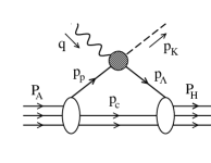
Figure 1: A schematic representation of the amplitude for photoproduction of a hypernucleus (H) induced by virtual photons in the plane-wave impulse approximation. The energy-momenta of the nucleus, denoted by A, and of the hypernucleus, denoted by H, are marked with capital letters ${\rm P}=(E,\vec{P}\,)$ and those of intermediate systems with lowercase letters.

This approach is justified because the photon and kaon momenta are supposed to be rather high ($\approx 1~{}\text{GeV}$), e.g., in the JLab experiments archival ; HallC , and this clearly separates the elementary production (the 2-body process) from the many-body reaction (1). The cross section for production of the ground and excited states of a hypernucleus depends on the many-particle matrix element between the nonrelativistic wave functions of the target nucleus ($\Psi_{A}$) and the hypernucleus ($\Psi_{H}$)

$${\sf M}_{\mu}=\langle\Psi_{H}|\langle\chi_{K}|\sum_{j=1}^{\sf Z}\;\hat{\rm\!J}_{\mu}(j)\,|\chi_{\gamma}\rangle|\Psi_{A}\rangle\,,$$ (2)

where $\chi_{K}$ is taken as a kaon plane (PWIA) or distorted (DWIA) wave function and $\hat{\rm\!J}_{\mu}(j)$ is an elementary operator for $\Lambda$ production on the $j$th proton. In the one-photon approximation without Coulomb distortion of initial and final electrons, the virtual-photon wave function $\chi_{\gamma}$ is taken as the plane wave. Due to the symmetry of the nuclear wave function, we can replace the sum over all protons with ${\sf Z}\;\hat{\rm\!J}_{\mu}$ where ${\sf Z}$ is the atomic number of the target nucleus. Denoting the intermediate momenta of the proton and $\Lambda$ as $\vec{p}_{p}$ and $\vec{p}_{\Lambda}$, respectively, the momentum transfer as $\vec{\Delta}=\vec{q}-\vec{p}_{K}$, and considering translational invariance, we introduce the elementary amplitude ${\cal J}_{\mu}(\vec{p}_{K},\vec{q},\vec{p}_{p})$

$$\langle\vec{p}_{K},\vec{p}_{\Lambda}\,|\,\hat{\rm\!J}_{\mu}|\,\vec{q},\vec{p}_{p}\rangle=(2\pi)^{3}\,\delta^{(3)}(\vec{p}_{\Lambda}-\vec{p}_{p}-\vec{\Delta})\,{\cal J}_{\mu},$$ (3)

which has to be expressed in the two-component form to match it with the nonrelativistic nuclear and hypernuclear wave functions in Eq. (2). Similarly, we introduce the hypernuclear production amplitude ${\cal T}_{\mu}(\vec{p}_{K},\vec{q},\vec{P}_{A})$

$${\sf M}_{\mu}=(2\pi)^{3}\,\delta^{(3)}(\vec{P}_{H}-\vec{P}_{A}-\vec{\Delta})\,{\cal T}_{\mu}\,.$$ (4)

In the nucleus-rest (lab) frame, this amplitude is

$$\!\!\!{\cal T_{\mu}}\! = \!\!{\sf Z}\!\int\!d^{3}\xi_{\Lambda}\,d^{3}\xi_{p}\,\exp\,(iB\,\vec{\Delta}\cdot\vec{\xi}_{\Lambda})\;\chi^{*}_{K}(\vec{p}_{KH},B\vec{\xi}_{\Lambda})$$ (5)

$$\times \int\!\frac{d^{3}p_{p}}{(2\pi)^{3}}\exp\biggl{[}i\vec{p}_{p}\cdot(\vec{\xi}_{\Lambda}-\vec{\xi}_{p})\biggr{]}\,{\sf Tr}\!\left[\!\frac{}{}\!{\cal J}_{\mu}(\vec{p}_{K},\vec{q},\vec{p}_{p})\right.$$

$$\times \int\!d^{3}\xi_{1}\,...\,d^{3}\,\xi_{A-2}\;\Phi^{*}_{\sf H}(\vec{\xi}_{1},\,...\,\vec{\xi}_{A-2},\vec{\xi}_{\Lambda})$$

$$\times \;\;\;\left.\Phi_{\sf A}(\vec{\xi}_{1},\,...\,\vec{\xi}_{A-2},\vec{\xi}_{p})\right]\,.$$

where $B=(A-1)/(A-1+m_{\Lambda}/m_{p})$, $\xi$’s are the Jacobi coordinates, and $\chi^{*}_{K}$ describes the kaon distortion ($\chi^{*}_{K}=1$ in PWIA) that depends on the kaon relative momentum with respect to the hypernucleus, $\vec{p}_{KH}$. The trace is over the proton and $\Lambda$ spin as ${\cal J}_{\mu}$ is the $2\times 2$ matrix in that space. The integral over the proton momentum $\vec{p}_{p}$ includes averaging over the Fermi motion of the target protons inside the nucleus. However, we can assume that a dependence on $\vec{p}_{p}$ in the amplitude ${\cal J}_{\mu}$ is much smoother than that in the phase factor weighted by the nuclear wave functions and take the elementary amplitude out of the integral for some effective (optimal) value of $\vec{p}_{p}$; i.e., we can replace ${\cal J}_{\mu}(\vec{p}_{K},\vec{q},\vec{p}_{p})$ with ${\cal J}_{\mu}(\vec{p}_{K},\vec{q},\vec{p}_{\sf eff})$. The integration over $\vec{p}_{p}$ then gives a $\delta$-function which allows integration over $\vec{\xi}_{\Lambda}$. Finally we arrive at an expression for the lab amplitude in the optimal factorization approximation (OFA) (see also FM-proton )

$$\!\!\!\!\!\!{\cal T_{\mu}}={\sf Z}\,{\sf Tr}\left[{\cal J}_{\mu}(\vec{p}_{K},\vec{q},\vec{p}_{\sf eff})\!\int\!d^{3}\xi\,e^{(iB\,\vec{\Delta}\cdot\vec{\xi})}\,\chi^{*}_{K}(\vec{p}_{KH},B\vec{\xi})\right.$$

$$\times \!\!\!\!\left.\int\!d^{3}\xi_{1}...d^{3}\,\xi_{A-2}\Phi^{*}_{\sf H}(\vec{\xi}_{1},...\,\vec{\xi}_{A-2},\vec{\xi}\,)\Phi_{\sf A}(\vec{\xi}_{1},...\,\vec{\xi}_{A-2},\vec{\xi}\,)\right],$$

where we omit a subscript at the integration variable $\vec{\xi}$ (as $\vec{\xi}_{p}=\vec{\xi}_{\Lambda}$) and $\vec{p}_{\sf eff}$ is an effective proton momentum. Recall that $\vec{\xi}$ is the relative particle-core coordinate.

In the previous calculations, see e.g. Refs. SF1994 ; archival ; Motoba , the effective momentum was set to zero in the so-called frozen-proton approximation. This choice provides us with a simple expression for the two-component (CGLN) elementary amplitude in the proton laboratory frame, see Eq. $(4.3)$ in SF1994 . Here the CGLN amplitude consists only of six structures. In the more general case with a non zero $\vec{p}_{\sf eff}$ one needs a more general CGLN-like form. In the next section we are going to derive this form which will allow us to go beyond the frozen-proton approximation.

II.2 Two-component elementary amplitude

Here we will present the two-component formalism for kaon electroproduction but it can be also applied for electroproduction of any pseudo-scalar meson.

The invariant amplitude of K⁺ production on a free proton induced by a virtual photon

$$\gamma_{\sf v}(q,\varepsilon)+{\sf p}(p_{p},\eta_{p})\longrightarrow\Lambda(p_{\Lambda},\eta_{\Lambda})+{\sf K^{+}}(p_{K})\,,$$ (7)

can be expressed via six gauge invariant (GI) operators

$${\cal M}^{\mu}\varepsilon_{\mu}=\bar{u}(p_{\Lambda},\eta_{\Lambda})\,\gamma_{5}\,\sum_{j=1}^{6}{\sf M}_{j}\,A_{j}(q^{2},s,t)\,u(p_{p},\eta_{p})$$ (8)

where, in the one-photon approximation, the electron part enters via the four-vector $\varepsilon_{\mu}=\frac{e}{q^{2}}\bar{u}(p^{\prime}_{e})\,\gamma_{\mu}u(p_{e})$ and the mass of the virtual photon is $q^{2}<0$. Dirac bispinors $\bar{u}_{\Lambda}$ and $u_{p}$ with spin projections $\eta_{\Lambda}$ and $\eta_{p}$ are for the $\Lambda$ and proton, respectively. The scalar amplitudes $A_{j}$ are functions of Mandelstam variables $s=(q+p_{p})^{2}$ and $t=(q-p_{K})^{2}$ and describe the reaction dynamics. They are obtained from a decomposition of contributions from Feynman diagrams SB16 ; SB18 . The GI operators ${\sf M}_{j}$, composed of $q$, $p_{p}$, $p_{\Lambda}$, $\varepsilon_{\mu}$, and $\gamma$-matrixes, assure that the invariant amplitude (8) fulfills the Ward identity ${\cal M}\cdot q=0$. Formulas for ${\sf M}_{j}$ are given in Eqs. (17) of Ref. SB16 . Specific expressions for the scalar amplitudes $A_{j}(s,t)$ and more details on the formalism in photo- and electroproduction of kaons can be found in Refs. SB16 ; SB18 .

The invariant amplitude (8) can be used to calculate observable quantities of the process (7) in any reference frame but it cannot be directly used to calculate the many-particle matrix element (2). For computing this matrix element we need a one-body transition operator on the nonrelativistic proton-hyperon Hilbert space written in the two-component formalism, i.e. using Pauli matrices. Only then can we fold the operator with the nuclear and hypernuclear nonrelativistic wave functions that are expressed by Pauli spinors. Moreover, as we see in Eq. (LABEL:matrix-5) we need the elementary amplitude, in general, for a nonzero proton momentum $\vec{p}_{\sf eff}$. Formulas for this two-component (CGLN) amplitude in special cases are already available in literature, see e.g. Ref. SF1994 for either the laboratory ($\vec{p}_{\text{eff}}=0$) or the center-of-mass ($\vec{p}_{\text{eff}}=-\vec{q}$) frame. Here we provide the two-component form of the amplitude for arbitrary value of the proton momentum, i.e., in an arbitrary frame.

Due to the GI of the amplitude (8) one can change the polarization vector $\epsilon_{\mu}=\varepsilon_{\mu}-\varepsilon_{0}\,q_{\mu}/q_{0}=(\,0,\,\vec{\epsilon}\;)$, which sets the time component to zero, and the amplitude can be written via a two-component amplitude $\vec{J}\cdot\vec{\epsilon}$,

$${\cal M}\cdot\varepsilon=\bar{u}_{\Lambda}\gamma_{5}\sum_{j=1}^{6}{\sf M}_{j}\,A_{j}\,u_{p}={\sf X}_{\Lambda}^{\dagger}\ (\vec{J}\cdot\vec{\epsilon}\,)\ \;{\sf X}_{p}\,,$$ (9)

where ${\sf X_{\Lambda}}^{\dagger}$ and ${\sf X}_{p}$ are Pauli spinors. The new form $\vec{J}$ includes nonrelativistic structures composed from Pauli matrices and three-momenta, for example $\vec{q}$, $\vec{p}_{K}$, and $\vec{p}_{p}$. After some manipulations we can arrive at the amplitude in the two-component form for a nonzero proton momentum $\vec{p}_{p}$,

$$\vec{J}\cdot\vec{\epsilon} = G_{1}\,(\vec{\sigma}\cdot\vec{\epsilon}\,)+G_{2}\,i(\vec{p}_{p}\times\vec{q}\cdot\vec{\epsilon}\,)+G_{3}\,i(\vec{p}_{K}\times\vec{q}\cdot\vec{\epsilon}\,)$$ (10)

$$+ G_{4}\,i(\vec{p}_{p}\times\vec{p_{K}}\cdot\vec{\epsilon}\,)+\ i(\vec{p}_{p}\times\vec{p}_{K}\cdot\vec{q}\,)\;\left[\,G_{5}\,(\vec{q}\cdot\vec{\epsilon}\,)\right.$$

$$+ \left.G_{6}\,(\vec{p}_{p}\cdot\vec{\epsilon}\,)+G_{7}\,(\vec{p}_{K}\cdot\vec{\epsilon}\,)\,\right]+\ G_{8}\,(\vec{\sigma}\cdot\vec{q}\,)(\vec{q}\cdot\vec{\epsilon}\,)$$

$$+ G_{9}\,(\vec{\sigma}\cdot\vec{q}\,)(\vec{p}_{p}\cdot\vec{\epsilon}\,)+G_{10}\,(\vec{\sigma}\cdot\vec{q}\,)(\vec{p}_{K}\cdot\vec{\epsilon}\,)$$

$$+ \ G_{11}\,(\vec{\sigma}\cdot\vec{p}_{p})(\vec{q}\cdot\vec{\epsilon}\,)+G_{12}\,(\vec{\sigma}\cdot\vec{p}_{p})(\vec{p}_{p}\cdot\vec{\epsilon}\,)$$

$$+ G_{13}\,(\vec{\sigma}\cdot\vec{p}_{p})(\vec{p}_{K}\cdot\vec{\epsilon}\,)+\ G_{14}\,(\vec{\sigma}\cdot\vec{p}_{K})(\vec{q}\cdot\vec{\epsilon}\,)$$

$$+ G_{15}\,(\vec{\sigma}\cdot\vec{p}_{K})(\vec{p}_{p}\cdot\vec{\epsilon}\,)+G_{16}\,(\vec{\sigma}\cdot\vec{p}_{K})(\vec{p}_{K}\cdot\vec{\epsilon}\,)\,.$$

Expressions for the CGLN-like amplitudes $G_{j}$ in terms of the scalar amplitudes $A_{j}$ and kinematical variables are given in Appendix A. In the special case of $\vec{p}_{p}=0$ one obtains the ordinary amplitude in the laboratory frame

$$\vec{J}_{L}\cdot\vec{\epsilon} = G_{1}\,(\vec{\sigma}\cdot\vec{\epsilon}\,)+G_{3}\,i(\vec{p}_{K}\times\vec{q}\cdot\vec{\epsilon}\,)$$

$$+ G_{8}\,(\vec{\sigma}\cdot\vec{q}\,)(\vec{q}\cdot\vec{\epsilon}\,)+G_{10}\,(\vec{\sigma}\cdot\vec{q}\,)(\vec{p}_{K}\cdot\vec{\epsilon}\,)$$

$$+ G_{14}\,(\vec{\sigma}\cdot\vec{p}_{K})(\vec{q}\cdot\vec{\epsilon}\,)+G_{16}\,(\vec{\sigma}\cdot\vec{p}_{K})(\vec{p}_{K}\cdot\vec{\epsilon}\,)\,,$$

which is equivalent to Eq. ($4.3$) of SF1994 and which was used in the DWIA calculations of the hypernuclear cross sections in Refs. archival ; AIP2018 . The formulas for $G_{j}$ agree with the corresponding formulas for $F_{i}$ ($i=$1,…6) in Eqs. (B$\cdot$3) of Ref. SF1994 . Similarly, we can compare Eq. (10) for the center-of-mass frame ($\vec{p}_{p}=-\vec{q}$) with that in Ref. SF1994 and with corresponding CGLN amplitudes in (B$\cdot$1) SF1994 .

In evaluating the matrix element (2) it is convenient to use the spherical form of the amplitude

$$\vec{J}\cdot\vec{\epsilon} = \!-\sqrt{3}\,[\,J^{(1)}\otimes\epsilon^{(1)}\,]^{0}=\sum_{\lambda}(-1)^{-\lambda}\,J^{(1)}_{\lambda}\epsilon^{(1)}_{-\lambda}\,,\;\;\;\;$$ (12)

where the components $J^{(1)}_{\lambda}$ are defined via 12 spherical amplitudes ${\cal F}^{S}_{\lambda\eta}$ with $S=0,1$ and $\lambda,\eta=\pm 1,0$:

$$J^{(1)}_{\lambda}=\sum_{S\eta}\,{\cal F}^{S}_{\lambda\eta}\,\sigma^{S}_{\eta}\,.$$ (13)

Here $\sigma^{1}_{\eta}$ are the spherical components of Pauli matrices and $\sigma^{0}_{0}$ is the unit matrix. Inserting (13) into (12) we get the following explicit form

$$\vec{J}\cdot\vec{\epsilon}= - \!\!\epsilon^{\;1}_{\;1}\;(\,{\cal F}^{\;0}_{\!\!-10}+\sigma^{1}_{\;1}\,{\cal F}^{\;1}_{\!\!-11}+\sigma^{1}_{0}\,{\cal F}^{\;1}_{\!\!-10}+\sigma^{1}_{\!-1}\,{\cal F}^{\;1}_{\!\!-1-1}\,)$$

$$+ \!\!\epsilon^{\;1}_{\;0}\;(\,{\cal F}^{\,0}_{00}\;\,+\sigma^{1}_{1}\,{\cal F}^{\,1}_{01}\;+\sigma^{1}_{0}\,{\cal F}^{\,1}_{00}\;+\sigma^{1}_{\!-1}\,{\cal F}^{\;1}_{0-1}\,)$$

$$- \!\!\epsilon^{\;1}_{-1}\,(\,{\cal F}^{\,0}_{10}\;+\sigma^{1}_{1}\,{\cal F}^{\,1}_{11}\;+\sigma^{1}_{0}\,{\cal F}^{\,1}_{10}\;+\sigma^{1}_{\!-1}\,{\cal F}^{\;1}_{1-1}\,)\,.$$

The formulas for ${\cal F}^{S}_{\lambda\eta}$ written in terms of the spherical components of the momenta and the CGLN-like amplitudes $G_{j}$ are given in Appendix B.

II.3 Cross section for hypernuclear production

The spherical components ($T^{(1)}_{\lambda}$) of the hypernuclear production amplitude (${\cal T}_{\mu}$) can be decomposed into the reduced amplitudes $A^{\lambda}_{Jm}$

$$T^{(1)}_{\lambda}=\frac{1}{[J_{H}]}\sum_{Jm}\,{\sf C}^{J_{H}M_{H}}_{J_{A}M_{A}Jm}\,A^{\lambda}_{Jm}\,,$$ (15)

where ${\sf C}^{J_{H}M_{H}}_{J_{A}M_{A}Jm}$ is the Clebsch-Gordan coefficient, ($J_{A}$, $M_{A}$) and ($J_{H}$, $M_{H}$) are the nuclear and hypernuclear spin and its projection, respectively, and $[J]=\sqrt{2J+1}$, which is used also in the following relations. In the OFA (LABEL:matrix-5) and assuming that the proton and $\Lambda$ are in single-particle states $\alpha$ ($=nlj$) and $\alpha^{\prime}$, respectively, we get

$$A^{\lambda}_{Jm}= \frac{1}{[J]}\,\sum_{S\eta}\,{\cal F}^{S}_{\lambda\eta}\,\sum_{LM}\;{\sf C}^{Jm}_{LMS\eta}\sum_{\alpha^{\prime}\alpha}{\cal R}^{LM}_{\alpha^{\prime}\alpha}\;{\cal H}^{LSJ}_{l^{\prime}j^{\prime}lj}$$ (16)

$$\times(\,\Phi_{H}\,||\,[b_{\alpha^{\prime}}^{+}\otimes a_{\alpha}]^{J}\,||\;\Phi_{A}\,)\,,$$

where ${\cal R}^{LM}_{\alpha^{\prime}\alpha}$ are the radial integrals, ${\cal H}^{LSJ}_{l^{\prime}j^{\prime}lj}$ includes the Racah algebra (see Eq. (37)), and the reduced one-body density matrix elements (OBDME) are non zero only for the considered single-particle transitions $(\alpha)_{p}\to(\alpha^{\prime})_{\Lambda}$ described by the operator $[b_{\alpha^{\prime}}^{+}\otimes a_{\alpha}]^{J}$ with the proton annihilation ($a_{\alpha}$) and $\Lambda$ creation ($b^{+}_{\alpha^{\prime}}$) operators. More details on derivation of Eq. (16) is given in Appendix C.

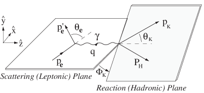
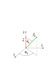
Figure 2: The laboratory frame for hypernucleus electroproduction ($\vec{P}_{A}=0$) with the $z$-axis oriented along the photon momentum $\vec{q}$. The $y$-axis of the right-handed system is perpendicular to the leptonic plane, see the upper part of the figure. The kaon momentum is defined by its polar $\theta_{K}$ and azimutal $\Phi_{K}$ angles, see the lower part. Similar notation is used for the proton momentum $\vec{p}_{p}$. The angle $\Phi_{K}$ also defines the angle between the leptonic and hadronic planes. Note our convention that for $\Phi_{K}=0$ the kaon momentum lies between the beam ($\vec{p}_{e}$) and photon momenta.

The cross sections are calculated in the laboratory frame ($\vec{P}_{A}=0$) with electron kinematics and definitions of the angles as given in Fig. 2. The virtual photon has the energy $E_{\gamma}=E_{e}-E_{e}^{\prime}$, a “mass” $Q^{2}=-q^{2}=\vec{q}^{\;2}-E_{\gamma}^{2}$, the transverse polarization

$$\varepsilon=\left(1+\frac{2|\vec{q}|^{2}}{Q^{2}}\,\text{tan}^{2}\frac{\theta_{e}}{2}\right)^{-1}\,,$$ (17)

and the longitudinal polarization given as $\varepsilon_{L}=\varepsilon\,Q^{2}/E_{\gamma}^{2}$. The unpolarized differential cross section for electroproduction is then

$$\frac{d\sigma}{d\Omega_{K}}=\frac{d\sigma_{\sf T}}{d\Omega_{K}}+\varepsilon_{L}\frac{d\sigma_{\sf L}}{d\Omega_{K}}+\varepsilon\frac{d\sigma_{\sf TT}}{d\Omega_{K}}+\sqrt{\varepsilon_{L}(\varepsilon+1)}\frac{d\sigma_{\sf TL}}{d\Omega_{K}},$$

$$\frac{d^{3}\sigma}{dE_{e}^{\prime}d\Omega_{e}^{\prime}d\Omega_{K}}=\Gamma\,\frac{d\sigma}{d\Omega_{K}}\,,\ \ \ \ \ \ \ \ \ \ \ \ \ \ \ \ \ \ \ \ \$$ (18)

where the triple-differential cross section is a product of $\text{d}\sigma/\text{d}\Omega_{K}$ and the virtual-photon flux in the nucleus-rest frame

$$\Gamma=\frac{\alpha}{2\pi^{2}}\frac{|\vec{q}\,|}{Q^{2}(1-\varepsilon)}\frac{E_{e}^{\prime}}{E_{e}}\,,$$ (19)

with the fine-structure constant $\alpha$. The separated cross sections are

$$\frac{d\sigma_{\sf T}}{d\Omega_{K}} =\frac{\beta}{2[J_{A}]^{2}}\sum_{Jm}\frac{1}{[J]^{2}}\left(\,|A^{+1}_{Jm}|^{2}+|A^{-1}_{Jm}|^{2}\right)\,,$$ (20a)

$$\frac{d\sigma_{\sf L}}{d\Omega_{K}} =\frac{\beta}{[J_{A}]^{2}}\sum_{Jm}\frac{1}{[J]^{2}}\,|A^{0}_{Jm}|^{2}\,,$$ (20b)

$$\frac{d\sigma_{\sf TT}}{d\Omega_{K}} =\frac{\beta}{[J_{A}]^{2}}\sum_{Jm}\frac{1}{[J]^{2}}\,{\sf Re\,}[A^{+1}_{Jm}A^{-1*}_{Jm}]\,,$$ (20c)

$$\frac{d\sigma_{\sf TL}}{d\Omega_{K}} =\frac{\beta}{[J_{A}]^{2}}\sum_{Jm}\frac{1}{[J]^{2}}\,{\sf Re\,}[A^{0*}_{Jm}(A^{+1}_{Jm}-A^{-1}_{Jm})]\,,$$ (20d)

where the kinematical factor $\beta$ depends on the kaon momentum SF1994 . In the kinematics considered here and those of the performed experiments archival the transverse part $d\sigma_{\sf T}$ dominates the cross section. The longitudinal part $d\sigma_{\sf L}$ gives small contributions but, as we will show, it is sensitive to kinematical effects and elementary amplitudes. The TL interference part is an important contribution to the full cross section even for quite small photon virtualities considered here, $Q^{2}\approx 0.01$ (GeV/c)².

II.4 Optimum on-shell approximation

The elementary electroproduction amplitude is constructed assuming that the involved particles are on their mass shell, except the virtual photon, and that the energy-momentum is conserved. However, in the impulse approximation (Fig. 1) the initial proton and final $\Lambda$ are not asymptotically free objects, in fact they are intermediate particles. In our model calculations we deem that it is reasonable to keep the baryons on their mass shell and consider a translational invariance of the elementary and overall amplitudes and of the nuclear and hypernuclear wave functions, the latter being written as a plane wave for the center-of-inertia motion multiplied by the internal part as a function of relative (Jacobi) coordinates. We also require energy conservation in the elementary vertex

$$E_{\gamma}+\sqrt{m_{p}^{2}+\vec{p}_{p}^{\;2}}=\sqrt{m_{K}^{2}+\vec{p}_{K}^{\;2}}+\sqrt{m_{\Lambda}^{2}+\vec{p}_{\Lambda}^{\;2}}$$ (21)

to keep the amplitude on the energy shell as well. This requirement together with energy conservation in many-body vertexes

$$E_{A} =\sqrt{M_{c}^{2}+(\vec{P}_{A}-\vec{p}_{p})^{2}}+\sqrt{m_{p}^{2}+\vec{p}_{p}^{\;2}}+\epsilon_{p}\,,$$ (22a)

$$E_{H} =\sqrt{M_{c}^{2}+(\vec{P}_{A}-\vec{p}_{p})^{2}}+\sqrt{m_{\Lambda}^{2}+\vec{p}_{\Lambda}^{\,2}}+\epsilon_{\Lambda}\,,$$ (22b)

where $\epsilon_{p}$ and $\epsilon_{\Lambda}$ are single-particle binding energies in a general reference frame, leads to a violation of the overall energy conservation by a factor $\epsilon_{p}-\epsilon_{\Lambda}$. However, as this difference is relatively small, $\epsilon_{p}-\epsilon_{\Lambda}\approx 10$ MeV, in comparison with the total energy, $E_{\gamma}+E_{A}\approx 10$ GeV, we neglect it assuming the overall energy conservation

$$E_{\gamma}+E_{A}=E_{K}+E_{H}\,.$$ (23)

The kinematics of electroproduction is determined by the virtual-photon momentum $q$ and polarization $\varepsilon$ and by the kaon polar $\theta_{K}$ and azimuthal $\Phi_{K}$ angles. The magnitude of the kaon three-momentum has to be calculated from energy conservation Eqs. (21) or (23), which we denote by $|\vec{p}_{K}(2b)|$ and $|\vec{p}_{K}(mb)|$, respectively. Since the solution $|\vec{p}_{K}(2b)|$ for the 2-body reaction with an arbitrary proton momentum in general differs from the solution $|\vec{p}_{K}(mb)|$ for the many-body process, we have to choose which value will be used in computing the elementary amplitude (ea) and the radial integral (ri) in Eq. (16) and for the kinematic factor $\beta$ in Eqs. (20a)–(20d). This provides us with various schemes of calculation:
(a) 2-body: only one value $|\vec{p}_{K}(2b)|$ is used for ea, ri, and $\beta$. The elementary amplitude is then on-energy-shell but the many body energy conservation (23) is violated.
(b) 2-body_ea: a hybrid scheme with two different values $|\vec{p}_{K}(2b)|$ for ea and $|\vec{p}_{K}(mb)|$ for ri and $\beta$. The elementary amplitude is on-energy-shell and both (21) and (23) are fulfilled. Note that this scheme was used in our previous calculations archival ; AIP2018 .
(c) many-body: only one value $|\vec{p}_{K}(mb)|$ is used for ea, ri, and $\beta$. However, in this case the elementary amplitude is off-energy-shell which causes additional uncertainty of the results.
In the next section we will show differences of the cross sections calculated in these schemes.

One can take advantage of the possibility to choose the effective value of $\vec{p}_{p}$ in Eq. (21) and find a value that gives the same solution as that of Eq. (23), $|\vec{p}_{K}(2b)|=|\vec{p}_{K}(mb)|$. This value exists and we denote it as an “optimum” proton momentum $\vec{p}_{\text{opt}}$. In fact, we have one equation for the magnitude $|\vec{p}_{\text{opt}}|$ and an angle with respect to $\vec{\Delta}$ which can be chosen. In our calculations we have chosen this angle to be 180^∘, i.e., the proton is moving opposite to the momentum transfer minimizing the momentum of $\Lambda$. Note that in the OFA, Eq. (LABEL:matrix-5), this optimum momentum equals $\vec{p}_{\text{eff}}$ and makes the three schemes given above equivalent allowing for the on-energy-shell elementary amplitude. Therefore we denote this as the optimum on-shell approximation. Note also that we do not perform an “optimal Fermi averaging” as in Ref. Harada for the ($\pi^{+}$, K⁺) production because we use the OFA.

II.5 Mean proton momentum in target nucleus

The effective value of the proton momentum in the OFA (LABEL:matrix-5) can be also chosen as a mean momentum of the proton determined from its mean kinetic energy inside a nucleus, $|\vec{p}_{\text{eff}}|=\sqrt{2\mu\,\langle E_{kin}\rangle}$, where $\mu$ is the reduced mass of the proton-core system. In the analysis presented here we calculate the mean kinetic energy of a proton inside ¹²C using the single-particle wave function of the proton used also for computing the radial integrals. The interaction between the proton and the core ¹¹B is described by the Woods-Saxon and Coulomb potential which was also used in Ref. archival . For the protons bound in the $0p_{1/2}$ and $0p_{3/2}$ states with the binding energies $-10.37$ and $-15.96$ MeV we have obtained the mean kinetic energies 18.15 MeV and 18.76 MeV, respectively. These very near values, even if the binding energies are quite different, can be attributed to a relatively strong spin-orbital part of the potential with a depth of $V_{LS}=-19$ MeV. The mean momenta are then 176.7 and 179.6 MeV/c. In our comparison presented in the next section we will consider that $|\vec{p}_{\text{eff}}|=179$ MeV/c with two values of the angle with respect to the photon, $\theta_{\text{eff}}=0^{\circ}$ and 180^∘.

III Results

First, we give more details about the model calculations presented here mentioning also upgrades of the model with respect to the previous version and then we show kinematic and Fermi motion effects on the angular ($\theta_{Ke}$) and energy ($E_{\gamma}$) dependence of the cross sections in electroproduction of ${}^{12}_{~{}\Lambda}$B. We prefer to use the kaon angle with respect to the beam, $\theta_{Ke}$, instead of with respect to the photon, $\theta_{K}$, see Fig. 2. The results are presented only for selected hypernuclear states ($E_{x}$[MeV], ${\sf J^{P}}$): (0.0, 1^-) and (0.116, 2^-) with $\Lambda$ in $s$ orbit and (10.525, 1⁺), (11.059, 2⁺), and (11.132, 3⁺) with $\Lambda$ in $p$ orbit. It is interesting to mention a selection rule according to which contributions from the spin non-flip part of the elementary amplitude ${\cal F}^{0}_{\lambda 0}$ in Eq. (16) are only possible for the states $1^{-}$ and $2^{+}$ but they are missing in $2^{-}$, $1^{+}$, and $3^{+}$. However, in the kinematic region considered here, i.e. small kaon-photon angles $\theta_{K}$, the strength of the spin non-flip spherical amplitudes ${\cal F}^{0}_{\lambda 0}$ is very small and therefore one cannot expect big differences due to this selection rule. There is, however, another “dynamical” selection rule which will be mentioned below and which generates differences between the results for these two groups of states.

III.1 More details of the calculation

The elementary amplitude ${\cal F}^{S}_{\lambda\eta}$ used in eq. (16) is described by our recent BS3 isobar model SB18 and by the older SLA Saclay-Lyon model SLA . Note that SLA does not describe the new electroproduction data as well as BS3 SB18 mainly because these data were not available during its construction. The OBDME are taken from shell-model structure calculations by John Millener with a $\Lambda$N effective interaction JohnM similarly to our previous calculations archival ; AIP2018 . The kaon distortion included in the radial integrals is described in the eikonal approximation with the first-order optical potential constructed from the separable KN amplitude as in Ref. archival .

A new feature of the present calculations is that the radial integrals ${\cal R}^{LM}_{\alpha^{\prime}\alpha}$ are calculated with proper single-particle wave functions according to the quantum numbers $\alpha$ and $\alpha^{\prime}$ of assumed transitions given by OBDME. In the previous calculations we used only the radial integrals with the quantum numbers of dominant transitions. Another improvement is using the right relative particle-core coordinate described by the Jacobi coordinate $|\vec{\xi}|$ in the radial integrals. This allows one to calculate the proton and $\Lambda$ wave functions from the Schrödinger equation with a particle-core potential. Here we use the Woods-Saxon and Coulomb potentials as in archival . Note also that when checking the new computer code we found that in our old code there was a wrong sign at the Clebsch-Gordan coefficient with $J=3$ which significantly changed results for the corresponding states. We have also corrected for a tiny flaw in calculating the virtual-photon flux for hypernucleus electroproduction. These upgrades of the calculations make some differences which will be shown and discussed in Fig. 3 and Table 2.

The calculations are performed in the coplanar kinematics ($\Phi_{K}$ = 180^∘), see Fig. 2, close to that of the Hall A experiment archival with $Q^{2}$ = 0.06 (GeV/c)², $\varepsilon$ = 0.7, $E_{\gamma}\in(1.5,2.5)$ GeV, and $\theta_{Ke}\in(5^{\circ},14^{\circ})$.

III.2 Kinematic and Fermi motion effects in the cross sections

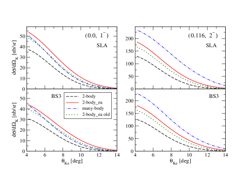
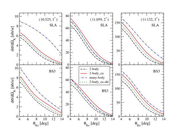
Figure 3: The full electroproduction cross section for the selected states of ${}^{12}_{~{}\Lambda}$B calculated in the frosen-proton approximation ($\vec{p}_{\sf eff}$ = 0) with the SLA and BS3 amplitudes and using various kaon momenta (computational schems). The results denoted as “2-body_ea old” are calculated without the upgrades in the radial integrals (see Sec. III.1) and therefore can be compared with our previous calculations in archival .

Kinematic effects caused by using different kaon momenta in schemes 2-body, 2-body_ea, and many-body are shown in Fig. 3 on the angular dependence of the full cross section $d\sigma/d\Omega_{K}$. The calculations are in the frozen-proton approximation ($\vec{p}_{\sf eff}=0$) with the photon energy $E_{\gamma}=2.2$ GeV. The upper and lower parts of the panels show results with the SLA and BS3 amplitudes, respectively, and each panel is for a given hypernuclear state. The result “2-body_ea old” was calculated with “absolute” coordinates in the radial integrals and with the radial integrals for the dominant transition ($\alpha\rightarrow\alpha^{\prime}$) as in our previous calculations archival . The absolute coordinates are suitable when we use the harmonic-oscillator single-particle wave functions but in calculations with the Woods-Saxon wave functions the relative particle-core (Jacobi) coordinates are more suitable. Comparison of the results “2-body_ea” and “2-body_ea old” therefore shows changes due to improvements in our model calculations. The new results are larger by a few per-cent.

The effects, given by different values of the kaon momentum $|\vec{p}_{K}|$ used in various components of the cross section, are quite large and do not depend much on the elementary amplitude. They are even larger in some cases for SLA than for BS3, see e.g. the results for the $1^{+}$ and $3^{+}$ states. Even if the difference between $|\vec{p}_{K}(2b)|$ and $|\vec{p}_{K}(mb)|$ in the considered kinematics and $\theta_{Ke}$ = 6^∘ is only smaller than 2%, the difference of corresponding momentum transfer $|\vec{\Delta}|$ is about 10%, which raises values of the radial integrals. Comparison of the results in the 2-body and 2-body_ea schemes show effects from the radial integrals and also from the normalization of the cross sections by the parameter $\beta$. As the angular dependence of $\beta$ is weak and $\beta[\vec{p}_{K}(mb)]>\beta[\vec{p}_{K}(2b)]$ the effect from $\beta$ is mainly the angle-independent rescaling of the cross section, which is observed for both elementary amplitudes and all states in Fig. 3. One can therefore conclude that even a small violation of the many-body energy conservation in the 2-body scheme makes the cross sections smaller by 10–20% for all states.

The effect of using the off-energy-shell elementary amplitude is seen from the comparison of the 2-body_ea (on-shell) and many-body (off-shell) schemes. In some cases, see e.g. the states $2^{-}$ and $1^{+}$ in Fig. 3, the effect is quite large, amounting to about 50% for $2^{-}$ at $\theta_{Ke}=6^{\circ}$, and, of-course, it depends on the amplitude. In general, bigger differences between the results are observed for the $2^{-}$, $1^{+}$, and $3^{+}$ states whereas the effects for the other group of states, $1^{-}$ and $2^{+}$ are smaller. Interestingly, the curves for the two groups of states, see e.g. states $1^{-}$ and $2^{-}$, are ordered in a different way. This feature can be understood from a numerical analysis of contributions to the reduced amplitude $A^{\lambda}_{Jm}$ in Eq. (16). Indeed, from the analysis one can conclude that the radial integrals with $M=0$ acquire the largest values, particularly their imaginary parts, and are rising functions of $|\vec{p}_{K}|$. Note also that $|\vec{p}_{K}(mb)|>|\vec{p}_{K}(2b)|$. Another observation is that the elementary amplitude ${\cal F}^{1}_{00}$ dominates in both 2-body_ea and many-body schemes. This dominance of contributions with $M=0$ and $\eta=0$ provides a selection rule given by values of the Clebsch-Gordan coefficient ${\sf C}^{J0}_{L010}$ in Eq. (16). Recall also that $J=J_{H}$ as $J_{A}=0$ for the ground state of ¹²C. This dynamical selection rule induces a dominance of the longitudinal amplitude $A^{0}_{20}$ for the $2^{-}$ state and therefore also a significant enhancement of the longitudinal (20b) and interference (20d) cross section. The large values of $d\sigma_{\sf L}$ and $d\sigma_{\sf TL}$ add up with $d\sigma_{\sf T}$ giving enhancement of the full cross section in the many-body scheme for the $2^{-}$ state for both SLA and BS3. On the other hand, in the $1^{-}$ state the amplitude $A^{0}_{10}=0$ due to the selection rule ${\sf C}^{10}_{1010}=0$ and the many-body cross section is even smaller than that in the 2-body_ea scheme. In this case the cross section is only given by the transverse part of the amplitude $A^{\pm 1}_{1m}$.

Table 1: Numerical results calculated with $Q^{2}=0.06$ (GeV/c)², $E_{\gamma}=2.2$ GeV, $\epsilon=0.7$, $\theta_{Ke}=6^{\circ}$, and $\Phi_{K}=180^{\circ}$ are shown for three computational schemes 2-body (2b), 2-body_ea (2b_ea), and many-body (mb). The full cross section (d$\sigma$) and contributions from the transverse (T), longitudinal (L), and interference (TL) parts are shown together with the reduced amplitudes with $\lambda=0$ and dominant components of the elementary amplitude BS3. The cross sections are in nb/sr. The bold values indicate the longitudinal contributions that constitute the selection rule.

Scheme	d$\sigma$	T	L	TL	$|A^{0}_{J\pm 1}|$	$|A^{0}_{J0}|$	${\cal F}^{1}_{00}$	${\cal F}^{1}_{01}=-{\cal F}^{1}_{0-1}$
			State $E=0.0$ MeV, $J^{P}=1^{-}$
2b	22.40	25.88	0.55	-4.21	0.165	0.0	(0.911, 2.529)	(-0.535, 0.203)
2b_ea	34.12	39.18	0.93	-6.24	0.213	0.0	(0.911, 2.529)	(-0.535, 0.203)
mb	30.34	38.75	1.48	-10.10	0.270	0.0	(-3.607, 3.114)	(0.108, 0.262)
			State $E=0.116$ MeV, $J^{P}=2^{-}$
2b	93.80	89.74	17.18	-13.71	0.364	1.610	(0.911, 2.529)	(-0.535, 0.203)
2b_ea	142.32	135.87	25.82	-20.26	0.461	1.947	(0.911, 2.529)	(-0.535, 0.203)
mb	187.77	134.46	77.59	-25.04	0.571	3.474	(-3.607, 3.114)	(0.108, 0.262)

In Table 1 we show numerical results for the cross sections, reduced amplitudes, and elementary amplitudes calculated with $\theta_{Ke}=6^{\circ}$ for the states $1^{-}$ and $2^{-}$. One can see a significant enhancement of $d\sigma_{\sf L}$ and $d\sigma_{\sf TL}$ for $2^{-}$ made by contributions from $|A^{0}_{20}|$. Note also a big value of the off-energy-shell elementary amplitude ${\cal F}^{1}_{00}$ in the many-body scheme. Similarly, the longitudinal cross section is enhanced in the states $1^{+}$ and $3^{+}$. From the dominance of the off-energy-shell elementary amplitude ${\cal F}^{1}_{00}$ one can also conclude, that the largest off-shell effects will be observed in $d\sigma_{\text{L}}$ and $d\sigma_{\text{TL}}$ as seen in Table 1. As the off-energy-shell extension of the elementary amplitude is barely under control we prefer the schemes 2-body and 2-body_ea with the on-energy-shell amplitude. Recall that if we opt for the optimum proton momentum, all schemes are equivalent and the elementary amplitude is on-energy-shell.

In the following we will study effects of the proton motion in the target nucleus, which we denote as Fermi motion effects. Particularly, we will demonstrate these effects on the angle and energy dependent cross sections calculated in the OFA with various effective proton momenta. We consider five cases:
i) frozen p $\vec{p}_{\sf eff}=0$ $\Rightarrow\vec{p}_{\Lambda}=\vec{\Delta}$ ii) frozen $\Lambda$ $\vec{p}_{\sf eff}=-\vec{\Delta}$ $\Rightarrow\vec{p}_{\Lambda}=0$ iii) optimum $\vec{p}_{\sf eff}=\vec{p}_{\sf opt}$ iv) mean 0 $|\vec{p}_{\sf eff}|=179$ MeV/c and $\theta_{p}=0^{\circ}$ v) mean 180 $|\vec{p}_{\sf eff}|=179$ MeV/c and $\theta_{p}=180^{\circ}$
Note that calculations in the frozen $\Lambda$ approximation were also performed in Ref. HLee for the ¹²C($\gamma$,K⁺)${}^{12}_{~{}\Lambda}$B reaction. The optimum and mean values are calculated as described in Secs. II.4 and II.5, respectively. We present the full cross section $d\sigma$ in Eq. (18) which corresponds to hypernuclear photoproduction induced by virtual photons. In the case of angular dependence the effects observed in $d\sigma$ qualitatively coincide with those in the triple-differential cross section $d^{3}\sigma$ because the virtual-photon flux factor $\Gamma$, Eq. (19), is kaon-angle independent and acts only as a scaling factor. In the case of the energy dependence the flux factor can modify the shape of the curves but as it depends only on the electron kinematics it does not qualitatively change effects due to different proton and kaon momenta.

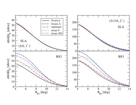
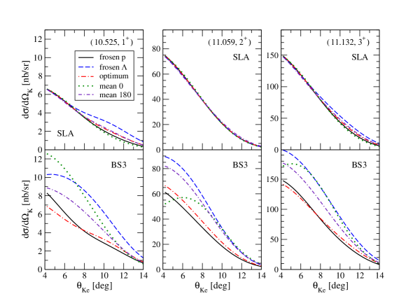
Figure 4: The full electroproduction cross section for the selected states of ${}^{12}_{~{}\Lambda}$B calculated in the scheme 2-body_ea with the SLA nad BS3 elementary amplitudes and with various values of the proton momentum $\vec{p}_{\sf eff}$. The photon has energy $E_{\gamma}$= 2.2 GeV, $Q^{2}$= 0.06 (GeV/c)², and polarization $\varepsilon$ = 0.7.

The results calculated in the 2-body_ea scheme with $E_{\gamma}=2.2$ GeV and with various proton momenta are shown in Fig. 4. The effects from the Fermi motion are very different, both in the magnitude and the shape, for the elementary amplitudes SLA and BS3. Whereas there are very small effects for the SLA (at given energy), the results with BS3 reveal quite a strong dependence on the proton momentum. The largest cross sections for a given state are obtained with the largest value of the momentum $|\vec{p}_{\sf eff}|=|\vec{\Delta}|\approx 300$ MeV/c in the case of frozen $\Lambda$, and the smallest values are with frozen proton, $|\vec{p}_{\sf eff}|=0$. These differences at small kaon angles, $\theta_{K}\approx 0$, make about 30% for BS3. Note that the BS3 results with the mean momentum strongly depend on the direction with respect to the photon momentum ($0^{\circ}$ or $180^{\circ}$) and that they reveal effects due to the dynamical selection rule. This angle dependence differs for the SLA nad BS3 amplitudes and it is more pronounced in the longitudinal components of the cross section as we will show below. The dependence of the effects on the elementary amplitude is also apparent from the result with the mean momentum and $\theta_{p}=0^{\circ}$ (the green dotted line) which lies mostly above the result with frozen proton (the black solid line) for the BS3 amplitude whereas it is slightly below the black line for the SLA amplitude. These effects survive for smaller energies ($E_{\gamma}=1.5$ GeV) where the Fermi motion effects with SLA are bigger. These observations suggest that the effects due to the proton motion depend on both the elementary amplitude and kinematics of the process.

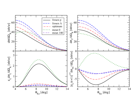
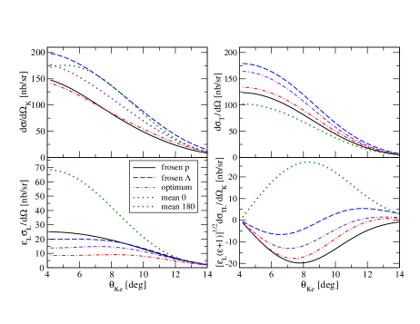
Figure 5: Contributions from the transverse (T), longitudinal (L), and transverse-longitudinal interference (TL) parts to the full cross section in Eq. (18) are shown for the ground state (upper panels) and the $3^{+}$ excited state (bottom panels) of ${}^{12}_{~{}\Lambda}$B. The results are calculated in the scheme 2-body_ea with the BS3 amplitude for the five values of the proton momentum and kinematics as in Fig. 4.

More pronounced effects of Fermi motion are observed in separated contributions from the transverse (T), longitudinal (L), and interference (TL) parts of the full cross section as it is shown in Fig. 5 for the BS3 amplitude and for the $1^{-}$ and $3^{+}$ states. Recall that the results for $1^{-}$ reveal similar features as those for $2^{+}$ and the results for $3^{+}$ are similar to those for $2^{-}$ and $1^{+}$. Figure 5 also shows a difference between the electro- and photoproduction calculations represented by the full $d\sigma$ for the former and by the transverse $d\sigma_{T}$ for the latter. The transverse part dominates the full cross section in the considered kinematic region (small $\theta_{\sf K}$ and $Q^{2}$), but the contributions from $d\sigma_{L}$ and $d\sigma_{TL}$ are also important corrections here, amounting to about 10% at 6–10 degrees. The particular contribution depends on the elementary amplitude. Note that the BS3 amplitude includes additional longitudinal couplings of the nucleon resonances to the virtual photon SB18 which are missing in the SLA amplitude. However, the results for the L and TL parts of the cross section calculated with SLA also reveal considerable effects due to the Fermi motion but these contributions largely cancel each other giving only tiny effects in the full electroproduction cross section.

Whereas the character of the results in Fig. 5 for the T contribution, the shape and ordering of the lines, is similar for both states, the magnitude and behaviour of the L contribution are strongly determined by the selection rule and nuclear structure. The interference part TL being also an important component of the full cross section reveals some differences for the presented states as well. Therefore, it is evident that the different character of the effects in the full cross sections for the $1^{-}$ and $3^{+}$ states is driven by the longitudinal component of the virtual photon. Recall that the longitudinal components of $d\sigma$ depend on the reduced amplitude $A^{0}_{Jm}$ with the largest value for $m=0$. Because also the longitudinal spherical amplitude ${\cal F}^{1}_{00}$ dominates (in this kinematic region), the behavior of $d\sigma_{L}$ is strongly affected by the selection rule for ${\sf C}^{J_{H}0}_{L010}$, e.g. ${\sf C}^{10}_{1010}=0\$ and ${\sf C}^{30}_{2010}=\sqrt{3/5}\$ for the states $1^{-}$ and $3^{+}$, respectively.

The effects of using various proton momenta in energy dependent cross section are shown in Figs. 6 and 7 for the calculations in the 2-body_ea scheme with $Q^{2}=0.06$ (GeV/c)², $\varepsilon=0.7$, $\Phi_{K}=180^{\circ}$, and $\theta_{Ke}=6^{\circ}$ changing the electron kinematics accordingly. The notation is the same as in Figs. 4 and 5, respectively.

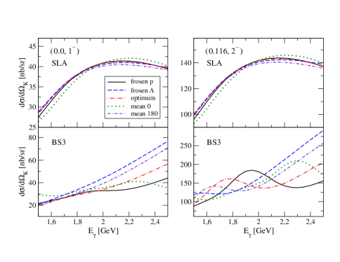
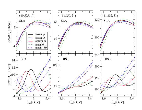
Figure 6: The same as in Fig. 4 but for energy dependence at kaon angle $\theta_{Ke}$ = 6^∘.

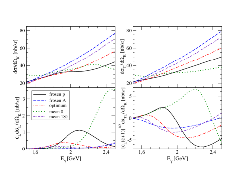
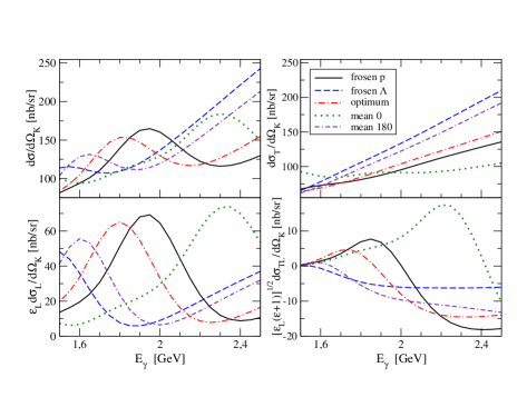
Figure 7: The same as in Fig. 5 but for energy dependence at kaon angle $\theta_{Ke}$ = 6^∘.

In Figure 6 we observe significant effects for both elementary amplitudes, especially at energies above 2 GeV. The resonant nature of the results for the states $2^{-}$, $1^{+}$, and $3^{+}$ comes from the longitudinal contributions, as shown in Fig. 7, and this structure is strongly controlled by the selection rule. A character of the results, i.e. ordering of the curves, is largely similar above 2 GeV and for a given amplitude but there are differences in a magnitude of the effects and in a particular shape of the curves. The shape depends quite strongly on the elementary amplitude but it also differs for the two groups of hypernuclear states which is related to the selective contribution from ${\cal F}^{1}_{00}$. Larger Fermi effects for SLA are observed in kinematics with $Q^{2}=0.01$ (GeV/c)² and $E_{\gamma}=1.5$ GeV than here, which is given by a magnitude of the effects in the spin-flip amplitude ${\cal F}^{1}_{\lambda\eta}$. In the case of the BS3 amplitude big effects are observed for both kinematics at energies above 2 GeV which is given by rising strength in the BS3 amplitude at higher energies as one can see in Figs. 5 and 11 of Ref. SB18 . For example, at $E_{\gamma}=2.4$ GeV the proton-photon invariant energy is 2.3 and 2.6 GeV in the frozen-proton and frozen-$\Lambda$ approximations, respectively, which makes the hypernuclear cross sections significantly larger for the latter. As the SLA amplitude provides almost a constant strength SB18 around 2 GeV, the Fermi effects are moderate in this energy region. Generally, the results with BS3 reveal more pronounced structures in the energy dependence than those with SLA. The structures are quite similar within the two groups of states, which is mainly driven by the contribution from the spin-flip part ${\cal F}^{1}_{\lambda\eta}$.

The resonant nature of the energy-dependent full cross section observed mainly for BS3 is induced by contributions from the longitudinal (L) and interference (TL) parts as one can clearly see in Fig. 7. The transverse part $d\sigma_{T}$ reveals a smooth energy dependence but the contributions from the L and TL parts model the resonant behavior in the full cross section, see the black (frozen proton) and red (optimum) lines for the $3^{+}$ state. Note that the behavior of the L and TL contributions significantly differs for the two extreme cases with the mean momentum, $\theta_{p}=0^{\circ}$ and $180^{\circ}$, which suggests that the contributions from the L and TL parts strongly depend on the angle between the proton and photon momenta.

Even if the energy behavior of the L and TL parts is quite similar for both states, see for example the results with the frozen proton and optimum momentum, the magnitude of their contributions differ quite strongly. The full cross sections at $E_{\gamma}=2$ GeV with frozen proton for the $1^{-}$ and $3^{+}$ states is about 30 and 150 nb/sr, respectively, and the contributions from L are about 1 and 60 nb/sr, respectively. The relative contribution from L then amounts to about 3% and 40% for the $1^{-}$ and $3^{+}$ states, respectively. This phenomenon can be attributed to a significant contribution from the elementary amplitude ${\cal F}^{1}_{00}$ in the longitudinal part for the $3^{+}$ state (where $A^{0}_{30}\neq 0$) which is absent in $1^{-}$ (where $A^{0}_{10}=0$). Note, however, that the contribution from L is smaller for energies different from approximately 2 GeV. The relatively large contribution from the longitudinal part at 2 GeV demonstrates again importance of the electroproduction calculations even in kinematics with a photon which is almost real ($Q^{2}=0.06$ (GeV/c)²).

In Figures 4–7 one sees that the results with the optimum proton momentum generally lie between the extreme cases with frozen proton and frozen $\Lambda$ and in most cases are close to the frozen proton approximation. Moreover, because in the version with the optimum momentum all the computational schemes are equivalent and calculations are performed with only one value of the kaon momentum, we suggest this version to be a suitable variant of the optimal factorization approximation in the DWIA and denote it as optimum on-shell approximation.

III.3 Comparison with data and previous results

In Table 2 we compare the new theoretical predictions for the triple-differential cross sections in electroproduction of ${}^{12}_{~{}\Lambda}$B with experimental data and our previous results (“old”), both from Table III of Ref. archival . The calculations are performed with the BS3 elementary amplitude in the following kinematics: $E_{e}=$ 3.77 GeV, $E_{e}^{\prime}=$ 1.56 GeV, $\theta_{e}=$ 6^∘, $\theta_{Ke}=$ 6^∘, $\Phi_{K}=$ 180^∘. The photon kinematics is $E_{\gamma}=$ 2.21 GeV, $Q^{2}=$ 0.0644 (GeV/c)², $\varepsilon=$ 0.7033, the photon angle with respect to the beam is 4.2^∘, and $\Gamma=$ 0.0178 (GeV/c)^-1 . The kaon angle with respect to the photon momentum is very small $\theta_{K}=$ 1.8^∘.

The new results “NEWa” are calculated in the frozen-proton approximation and the 2-body_ea scheme with two values of the kaon momentum $|\vec{p}_{K}(2b)|=1931$ MeV/c and $|\vec{p}_{K}(mb)|=1964$ MeV/c. The momentum of $\Lambda$ is 301 MeV/c and it equals the momentum transfer. The result “NEWb” is the same calculation as NEWa but with the optimum proton momentum $|\vec{p}_{\sf opt}|=$ 99 MeV/c and cos($\theta_{p\Delta}$)= $-1$. The kaon momentum is $|\vec{p}_{K}(2b)|=|\vec{p}_{K}(mb)|=$ 1964 MeV/c, the $\Lambda$ moves with momentum 170 MeV/c and the momentum transfer is $|\vec{\Delta}|=$ 269 MeV/c. One sees that the optimum momentum is comparable to the $\Lambda$ momentum and to $|\vec{\Delta}|$. We denote the calculation NEWb as the optimum on-shell approximation, see also Sec. II.4.

Data		Theoretical predictions
$E_{x}$	crs	$E_{x}$	JP	Cross sections
(MeV)		(MeV)		old	NEWa	NEWb
		0.000	1-	0.524	0.611	0.741
		0.116	2-	2.172	2.535	2.677
0.0	4.51	sum:		2.696	3.145	3.418
		2.587	1-	0.689	0.805	0.956
		2.593	0-	0.071	0.082	0.027
2.62	0.58	sum:		0.760	0.887	0.983
		4.761	2-	—	0.022	0.022
		5.642	2-	0.359	0.422	0.429
		5.717	1-	0.097	0.113	0.132
5.94	0.51	sum:		0.456	0.558	0.583
		10.480	2+	0.157	0.175	0.196
		10.525	1+	0.100	0.111	0.098
		11.059	2+	0.778	0.870	0.973
		11.132	3+	1.324	2.169	2.099
		11.674	1+	0.047	0.085	0.087
10.93	4.68	sum:		2.406	3.410	3.453
		12.967	2+	0.447	0.504	0.556
		13.074	1+	0.196	0.219	0.191
		13.383	1+	—	0.0008	0.0008
12.65	0.63	sum:		0.643	0.724	0.748

Table 2: Experimental cross sections (crs) for electroproduction of ${}^{12}_{~{}\Lambda}$B in nb/(sr²GeV) are compared with theoretical predictions calculaterd with the BS3 amplitude. The data and results “old” are from archival . The newly elaborated results (see Sec. III.1) “NEWa” and “NEWb” are calculated with the zero and the optimum proton momentum, respectively. The theoretical prediction on the line denoted with “sum:” is the total cross sections for given multiplet which can be compared with the experimental value.

The differences between the results “old” and “NEWa” observed in Table 2 are due to our improvements in the model calculations, especially in the radial integrals, see details of the calculation in Sec. III.1. A remarkable change is the markedly larger cross section for the state 3⁺ at 11.132 MeV which is mainly due to a flaw in the previous calculations. The new value significantly improves agreement with the data for the second dominant peak at 11 MeV. We can say that at the given energy the new cross sections for all states are larger by 10–15 % for both BS3 and SLA elementary amplitudes.

On the other hand, differences between the results with the zero (NEWa) and the optimum proton momentum (NEWb) depend quite strongly on the elementary amplitude. The new results with the optimum proton momentum are larger by 1–11% for BS3 as shown in Table 2 but the results with SLA are larger only by less than 1%. However, recall that the effects from the proton motion for SLA are larger for energies different from 2.21 GeV, e.g. for $E_{\gamma}=$ 1.5 and 2.4 GeV as seen in Fig. 6. Note also that the Fermi-motion effects in Table 2 are moderate due to a quite small value of the optimum proton momentum (99 MeV/c).

We can conclude that both the effects of the proton motion and the improvements of our model calculations lead to a better agreement of theoretical predictions NEWb with the data for both main peaks at 0 and 11 MeV. The new results are still about 27% below the experimental values for the main peaks whereas the new calculation overpredicts the cross sections for the other core-excited states. Let us note, however, that in the optimum on-shell approximation one uses only one value of the kaon momentum which allows for both the energy conservation in the overall system and the use of the on-energy-shell elementary amplitude. Recall also that the optimum momentum is not determined uniquely as it also depends on the angle between the proton momentum and the momentum transfer $\vec{\Delta}$. In our analysis we have considered only the special case with $\cos(\theta_{p\Delta})=-1$.

For completeness, in Tables 3 and 4 we also report on the new calculations with the BS3 amplitude for the hypernuclei ${}^{9}_{\Lambda}$Li and ${}^{16}_{~{}\Lambda}$N. These old results and the experimental data were already published in Ref. archival and here we compare them with the new results similarly to what we did for ${}^{12}_{~{}\Lambda}$B in Table II. One can see that the Fermi-motion effects due to optimum proton momentum raise the cross sections by 3–20% for ${}^{16}_{~{}\Lambda}$N ($p_{\sf opt}$= 120 MeV/c) and only by 4–6% for ${}^{9}_{\Lambda}$Li ($p_{\sf opt}$= 82 MeV/c). The smaller effects in the latter case can be partially attributed to the smaller value of the proton momentum. These effects together with improvements in the calculation make disagreement of the theoretical results with the data still worse for ${}^{16}_{~{}\Lambda}$N but they improve the agreement of theory and data for ${}^{9}_{\Lambda}$Li. Note that in the calculations with SLA, changes of the cross sections due to improvements are of similar magnitude but that the Fermi-motion effects are smaller.

Data		Theoretical predictions
$E_{x}$	crs	$E_{x}$	JP	Cross sections
(MeV)		(MeV)		old	NEWa	NEWb
0.0	0.59	0.000	3/2+	0.157	0.188	0.197
0.57	0.83	0.563	5/2+	1.035	1.238	1.314
sum:	1.42			1.19	1.43	1.51
		1.423	1/2+	0.294	0.353	0.399
		1.445	3/2+	0.343	0.412	0.398
1.45	0.79	sum:		0.64	0.77	0.80
		2.272	5/2+	0.109	0.130	0.147
		2.732	7/2+	0.315	0.379	0.382
2.27	0.54	sum:		0.42	0.51	0.53

Table 3: The same as in Table 2 but for ${}^{9}_{\Lambda}$Li.

Different results were obtained for ${}^{12}_{~{}\Lambda}$B at lower photon energy $E_{\gamma}=1.5$ GeV in kinematics of the Hall C experiment HallC where the Fermi-motion effects raise the cross sections by 2–4% for SLA but they lower them by about 6% for BS3. Note that the effects from improvements of the calculations are also important at this energy raising the cross sections which improves agreement of theoretical predictions with the data. This is illustrated in Table 5 where we compare the new results in the frozen-proton (NEWa) and optimum on-shell (NEWb) approximations with data from the Hall C experiment E01-011 and with our previous results published in Table VI of Ref. archival . We show only the results for $\Lambda$ in the $s$ orbit for which assignment of the theory and experimental data is straightforward. The differential cross sections were calculated at kinematics, $E_{e}=1.851$ GeV, $E_{e}^{\prime}=0.351$ GeV, $\theta_{e}=5.4^{\circ}$, $\theta_{Ke}=7.11^{\circ}$ and $\Phi_{K}=90^{\circ}$, with the elementary amplitude SLA SLA for which we obtained a better agreement with the data than with the BS3 amplitude. The new results with the optimum proton momentum (128 MeV/c) are in a better agreement with the data than the results with zero proton momentum. However, significant improvement comes from the changes in the model calculations, compare the results “old” and “NEWa”.

Data		Theoretical predictions
$E_{x}$	crs	$E_{x}$	JP	Cross sections
(MeV)		(MeV)		old	NEWa	NEWb
		0.000	0-	0.134	0.151	0.071
		0.023	1-	1.391	1.587	2.027
0.0	1.45	sum:		1.52	1.74	2.10
		6.730	1-	0.688	0.800	0.967
		6.978	2-	2.153	2.502	2.679
6.83	3.16	sum:		2.84	3.30	3.65
		11.000	2+	1.627	1.777	2.078
		11.116	1+	0.679	0.767	0.752
		11.249	1+	0.071	0.064	0.058
10.92	2.11	sum:		2.38	2.61	2.89
		17.303	1+	0.181	0.197	0.183
		17.515	3+	2.045	3.597	3.550
		17.567	2+	1.723	1.910	2.142
17.10	3.44	sum:		3.95	5.70	5.88

Table 4: The same as in Table 2 but for ${}^{16}_{~{}\Lambda}$N.

Data		Theoretical predictions
$E_{x}$	crs	$E_{x}$	JP	Cross sections
(MeV)		(MeV)		old	NEWa	NEWb
		0.000	1-	13.90	17.89	18.04
		0.116	2-	44.70	57.48	60.00
0.0	101.0	sum:		58.60	75.37	78.04
		2.587	1-	17.26	22.20	23.05
		2.593	0-	0.04	0.05	0.01
3.127	33.5	sum:		17.31	22.25	23.06
		4.761	2-	0.37	0.49	0.50
		5.642	2-	7.20	9.37	9.74
		5.717	1-	2.44	3.17	3.23
6.077	26.0	sum:		10.01	13.03	13.47

Table 5: Differential cross sections in nb/sr (crs) from the Hall C experiment E01-011 for electroproduction of ${}^{12}_{~{}\Lambda}$B are compared with theoretical predictions calculated with the SLA amplitude. Only the states with $\Lambda$ in the $s$ orbit are shown. The data are from HallC and the results “old” are from archival . The new results “NEWa” and “NEWb” are calculated with the zero and optimum proton momentum, respectively. The theoretical prediction on the line denoted with “sum:” is the total cross section for the given multiplet which can be compared with the experimental value.

IV Summary

We investigated the cross sections for electroproduction of ${}^{12}_{~{}\Lambda}$B and effects therein, which are caused by various options for kaon and proton momenta. The value of the kaon momentum is related to a choice of the computational scheme and the proton momentum relates to the Fermi motion of the target proton inside of the nucleus. The calculations were performed in the DWIA where the many-particle matrix element is treated in the optimal factorization approximation with an effective proton momentum in the elementary amplitude. In order to allow for non-zero values of the proton momentum, we have derived the two-component (CGLN-like) form of the elementary amplitude which applies generally for electroproduction of pseudo-scalar mesons off the nucleons. These CGLN-like amplitudes in a general reference frame can be calculated from known scalar amplitudes. Note that in the previous calculations the approximation with zero proton momentum (frozen proton) was considered and that, as far as we know, this general form of the electroproduction amplitude was not available in literature yet.

Utilizing this new formalism for the elementary amplitude with the nucleus-hypernucleus transition matrix elements (OBDME) and the kaon distortion as in our previous calculations archival we have found that the effects of various choices of the proton effective momentum (the Fermi motion effect) depend quite strongly on kinematics and the elementary amplitude. The effects are in general more pronounced for larger photon energies, i.e. above 2 GeV in the target-nucleus laboratory frame, which is given by the magnitude of the effects in the elementary amplitude. Generally, larger effects were observed for the BS3 amplitude, especially in the energy dependence of the cross sections. Resonant structures in the full cross section are modeled by contributions from the longitudinal (L) and transverse-longitudinal interference (TL) parts which reveal quite a strong sensitivity to the value of proton momentum.

The Fermi motion effects also differ for the hypernuclear states with various spins and parities due to the selective contribution from the strong longitudinal spherical elementary amplitude ${\cal F}^{1}_{00}$. We denote these noticeable differences of the results for two groups of hypernuclear states as the dynamical selection rule which enters into the full cross section mainly via the L and TL contributions. We can therefore conclude that the Fermi motion effects are very important for the L and TL contributions in the full cross section.

We have also shown that the cross section depends quite strongly on a scheme of computing the kaon laboratory momentum. If the kaon momentum is computed from the energy conservation in the elementary-production vertex, the elementary amplitude is on-energy-shell and the energy conservation of the overall system is violated by about 1%. On the contrary, calculations with the kaon momentum from the overall energy conservation have big effects in the elementary amplitude which is off-energy shell. The off-shell value of the dominant amplitude ${\cal F}^{1}_{00}$ differs significantly from the on-shell value resulting in large contributions in the L and TL components of the full cross section.

As the off-energy-shell extension of the elementary amplitude is generally not well under control, we prefer using the computational schemes with the on-energy-shell elementary amplitude. In the previous calculations we therefore considered a hybrid form with the on-energy-shell elementary amplitude and with the kaon momentum calculated from the overall energy conservation used in the remaining parts of the computation, i.e. two different kaon momenta were used. However, the new formalism for the elementary amplitude developed here allows to use an “optimum” proton momentum which makes the computational schemes equivalent, fulfilling both energy conservation relations with one value of the kaon momentum, and also allows us to use the on-energy-shell elementary amplitude.

This optimum on-shell approximation was shown to be a suitable choice of the effective proton momentum in the optimal factorization approximation in DWIA as the obtained results are in a better agreement with the experimental data. Note, however, that this improvement is also partially related to elaborating our model calculations. The optimum proton momentum used here for comparison with the experimental data on the ¹²C target amounts to about 100 MeV/c which is in a reasonable agreement with the mean value of the proton momentum in the $p$ orbit in ¹²C, about 180 MeV/c. We therefore suggest using this optimum on-shell approximation in DWIA calculations.

Note that as the optimum momentum is not determined uniquely, one could also try other values of the angle of the proton momentum with respect to the momentum transfer. The option used here with the proton moving opposite to the momentum transfer minimizes the momentum of the $\Lambda$.

Appendix A The CGLN-like amplitudes in a general reference frame

The CGLN-like amplitudes in Eq. (10) depend on the six scalar amplitudes $A_{j}$ SB18 and four-vectors $q=(q_{0},\vec{q}\,)$, $p_{p}=(E_{p},\vec{p}_{p})$, and $p_{\Lambda}=(E_{\Lambda},\vec{p}_{\Lambda})$. We denote the scalar product as $(a\cdot b)=a_{0}b_{0}-\vec{a}\,\vec{b}$. The amplitudes are normalised with $N=1/\sqrt{4m_{\Lambda}m_{p}(E_{\Lambda}+m_{\Lambda})(E_{p}+m_{p})}$ where $m_{p}$ and $m_{\Lambda}$ are proton and $\Lambda$ masses, respectively. Except for the photon (in electroproduction) the particles are on the mass shell, $m^{2}=E^{2}-\vec{p}^{\,2}$. The CGLN-like amplitudes in terms of the scalar amplitudes and kinematical variables read

$$G_{1} = N\left\{\frac{}{}\!\!\left[(p_{\Lambda}\cdot p_{p})\,q_{0}-m_{\Lambda}m_{p}\,q_{0}-(q\cdot p_{\Lambda})(E_{p}+m_{p})-(q\cdot p_{p})(E_{\Lambda}+m_{\Lambda})\right]A_{1}\right.$$

$$\left.\ \ \ \ +\left[(p_{\Lambda}\cdot p_{p})+m_{\Lambda}m_{p}+E_{\Lambda}m_{p}+E_{p}m_{\Lambda}\right]\left[(q\cdot p_{p})A_{4}+(q\cdot p_{\Lambda})A_{5}-q^{2}A_{6}\right]\frac{}{}\!\!\right\}\,,$$

$$G_{2} = N\left[\,(q_{0}+E_{p}+m_{p}-E_{\Lambda}-m_{\Lambda})A_{1}+(q\cdot p_{p})A_{4}+(q\cdot p_{\Lambda})A_{5}-q^{2}A_{6}\right]\,,$$

$$G_{3} = N\left[-(E_{p}+m_{p})A_{1}\,\right]\,,$$

$$G_{4} = N\left[-q_{0}\,A_{1}-(q\cdot p_{p})A_{4}-(q\cdot p_{\Lambda})A_{5}+q^{2}A_{6}\,\right]\,,$$

$$G_{5} = N\left[-A_{5}+A_{6}\,\right]\,,$$

$$G_{6} = N\left[-A_{4}-A_{5}\,\right]\,,$$

$$G_{7} = N\left[\,A_{5}\,\right]\,,$$

$$G_{8} = N\left\{\frac{}{}\!\!-(E_{p}+m_{p})A_{1}-\frac{E_{p}+m_{p}}{q^{2}}\left[(q\cdot p_{p})A_{2}+((q\cdot p_{\Lambda})-q^{2})A_{3}\right]\right.$$

$$\left.\ \ \ \ +\left[(p_{\Lambda}\cdot p_{p})-(q\cdot p_{p})+m_{p}(E_{\Lambda}+m_{\Lambda}-q_{0})+E_{p}\,m_{\Lambda}\right](A_{5}-A_{6})\frac{}{}\!\right\}\,,$$

$$G_{9} = N\left\{\frac{}{}\!(q_{0}-E_{p}-m_{p}-E_{\Lambda}-m_{\Lambda})A_{1}+(E_{p}+m_{p})(A_{2}+A_{3})\right.$$

$$\left.\ \ \ \ +\left[(p_{p}\cdot p_{\Lambda})+m_{p}(E_{\Lambda}+m_{\Lambda}-q_{0})+E_{p}\,m_{\Lambda}\right]A_{4}\right.$$

$$\left.\ \ \ \ +\left[(q\cdot p_{\Lambda})-(q\cdot p_{p})+(p_{p}\cdot p_{\Lambda})+m_{p}(E_{\Lambda}+m_{\Lambda}-q_{0})+E_{p}m_{\Lambda}\right]A_{5}-q^{2}A_{6}\frac{}{}\!\right\}\,,$$

$$G_{10} = N\left\{\frac{}{}\!(E_{p}+m_{p})(A_{1}-A_{3})+\left[(q\cdot p_{p})-(p_{p}\cdot p_{\Lambda})-m_{p}(E_{\Lambda}+m_{\Lambda}-q_{0})-E_{p}\,m_{\Lambda}\right]A_{5}\right\}\,,$$

$$G_{11} = N\left\{\frac{}{}\!\!q_{0}\,A_{1}+\frac{1}{q^{2}}(E_{\Lambda}+m_{\Lambda}-E_{p}-m_{p})\left[(q\cdot p_{p})A_{2}+((q\cdot p_{\Lambda})-q^{2})A_{3}\right]+(q\cdot p_{p})A_{4}-\right.$$

$$\left.\ \ \ \ -\left[(q\cdot p_{p})+q_{0}(m_{\Lambda}+m_{p})\right]A_{5}+\left[(q\cdot p_{p})+(q\cdot p_{\Lambda})-q^{2}+q_{0}(m_{\Lambda}+m_{p})\right]A_{6}\frac{}{}\!\right\}\,,$$

$$G_{12} = N\left\{\frac{}{}\!2\,q_{0}\,A_{1}+(E_{p}+m_{p}-E_{\Lambda}-m_{\Lambda})(A_{2}+A_{3})-q_{0}(m_{\Lambda}+m_{p})(A_{4}+A_{5})\right.$$

$$\left.-\left[(q\cdot p_{\Lambda})-(q\cdot p_{p})\right](A_{4}-A_{5})-2\,q^{2}A_{6}\frac{}{}\!\right\}\,,$$

$$G_{13} = N\left\{\frac{}{}\!\!\!-q_{0}\,A_{1}+(E_{\Lambda}+m_{\Lambda}-E_{p}-m_{p})A_{3}-(q\cdot p_{p})A_{4}+\left[(q\cdot p_{p})+q_{0}(m_{\Lambda}+m_{p})\right]A_{5}+q^{2}A_{6}\frac{}{}\!\right\}\,,$$

$$G_{14} = N\left\{\frac{E_{p}+m_{p}}{q^{2}}\left[(q\cdot p_{p})A_{2}+((q\cdot p_{\Lambda})-q^{2})A_{3}\right]+\left[(q\cdot p_{p})+q_{0}m_{p}\right](A_{5}-A_{6})\frac{}{}\!\right\}\,,$$

$$G_{15} = N\left\{\frac{}{}\!\!\!-q_{0}\,A_{1}-(E_{p}+m_{p})(A_{2}+A_{3})+q_{0}\,m_{p}A_{4}+\left[(q\cdot p_{p})+q_{0}\,m_{p}-(q\cdot p_{\Lambda})\right]A_{5}+q^{2}A_{6}\frac{}{}\!\right\}\,,$$

$$G_{16} = N\left\{\frac{}{}\!\!(E_{p}+m_{p})A_{3}-\left[(q\cdot p_{p})+q_{0}\,m_{p}\right]A_{5}\frac{}{}\!\right\}\,.$$

Appendix B The spherical amplitudes in a general reference frame

The non spin-flip ($S=0$) spherical amplitudes ${\cal F}^{S}_{\lambda\eta}$ in Eq. (13) can be written in terms of the CGLN-like amplitudes and spherical components of the photon ($\vec{q}$), proton ($\vec{p}_{p}$) and kaon ($\vec{p}_{K}$) momenta

$${\cal F}^{0}_{-10} = -|\vec{q}\,|\,[\,(p_{p})^{\;1}_{-1}\,G_{2}+(p_{K})^{\;1}_{-1}\,G_{3}\,]+[\,(p_{p})^{1}_{0}\;(p_{K})^{\;1}_{-1}-(p_{p})^{\;1}_{-1}\,(p_{K})^{1}_{0}\,]\,G_{4}+$$

$$+D\,[\,(p_{p})^{\;1}_{-1}\,G_{6}+(p_{K})^{\;1}_{-1}\,G_{7}\,]$$

$${\cal F}^{0}_{\,00} = -[\,(p_{p})^{\,1}_{-1}\;(p_{K})^{1}_{1}-(p_{p})^{1}_{1}\,(p_{K})^{\,1}_{-1}\,]\,G_{4}+D\,[\,|\vec{q}\,|\,G_{5}+(p_{p})^{1}_{0}\,G_{6}+(p_{K})^{1}_{0}\,G_{7}\,]$$

$${\cal F}^{0}_{\,10} = |\vec{q}\,|\,[\,(p_{p})^{1}_{1}\,G_{2}+(p_{K})^{1}_{1}\,G_{3}\,]-[\,(p_{p})^{1}_{0}\;(p_{K})^{1}_{1}-(p_{p})^{1}_{1}\,(p_{K})^{1}_{0}\,]\,G_{4}+$$

$$+D\,[\,(p_{p})^{1}_{1}\,G_{6}+(p_{K})^{1}_{1}\,G_{7}\,]$$

Similarly we can write down the spin flip ($S=1$) spherical amplitudes

$${\cal F}^{1}_{11} = G_{1}-(p_{p})^{\,1}_{-1}\,[\,(p_{p})^{1}_{1}\,G_{12}+(p_{K})^{1}_{1}\,G_{13}\,]-(p_{K})^{\,1}_{-1}\,[\,(p_{p})^{1}_{1}\,G_{15}+(p_{K})^{1}_{1}\,G_{16}\,]$$

$${\cal F}^{1}_{10} = |\vec{q}\,|\,[\,(p_{p})^{1}_{1}\,G_{9}+(p_{K})^{1}_{1}\,G_{10}\,]+(p_{p})^{1}_{0}\,[\,(p_{p})^{1}_{1}\,G_{12}+(p_{K})^{1}_{1}\,G_{13}\,]+$$

$$+(p_{K})^{1}_{0}\,[\,(p_{p})^{1}_{1}\,G_{15}+(p_{K})^{1}_{1}\,G_{16}\,]$$

$${\cal F}^{1}_{1-1} = -(p_{p})^{1}_{1}\,[\,(p_{p})^{1}_{1}\,G_{12}+(p_{K})^{1}_{1}\,G_{13}\,]-(p_{K})^{1}_{1}\,[\,(p_{p})^{1}_{1}\,G_{15}+(p_{K})^{1}_{1}\,G_{16}\,]$$

$${\cal F}^{1}_{01} = -|\vec{q}\,|\,[\,(p_{p})^{\,1}_{-1}\,G_{11}+(p_{K})^{\,1}_{-1}\,G_{14}\,]-(p_{p})^{1}_{0}\,[\,(p_{p})^{\,1}_{-1}\,G_{12}+(p_{K})^{\,1}_{-1}\,G_{15}\,]-$$

$$-(p_{K})^{1}_{0}\,[\,(p_{p})^{\,1}_{-1}\,G_{13}+(p_{K})^{\,1}_{-1}\,G_{16}\,]$$

$${\cal F}^{1}_{00} = G_{1}+|\vec{q}\,|\,[\,|\vec{q}\,|\,G_{8}+(p_{p})^{1}_{0}\,G_{9}+(p_{K})^{1}_{0}\,G_{10}+(p_{p})^{1}_{0}\,G_{11}+(p_{K})^{1}_{0}\,G_{14}\,]+$$

$$+(p_{p})^{1}_{0}\,(p_{p})^{1}_{0}\,G_{12}+(p_{p})^{1}_{0}\,(p_{K})^{1}_{0}\,(G_{13}+G_{15})+(p_{K})^{1}_{0}\,(p_{K})^{1}_{0}\,G_{16}$$

$${\cal F}^{1}_{0-1} = -|\vec{q}\,|\,[\,(p_{p})^{1}_{1}\,G_{11}+(p_{K})^{1}_{1}\,G_{14}\,]-(p_{p})^{1}_{1}\,[\,(p_{p})^{1}_{0}\,G_{12}+(p_{K})^{1}_{0}\,G_{13}\,]-$$

$$-(p_{K})^{1}_{1}\,[\,(p_{p})^{1}_{0}\,G_{15}+(p_{K})^{1}_{0}\,G_{16}\,]$$

$${\cal F}^{1}_{-11} = -[(p_{p})^{\,1}_{-1}\,(p_{p})^{\,1}_{-1}\,G_{12}+(p_{p})^{\,1}_{-1}\,(p_{K})^{\,1}_{-1}\,(G_{13}+G_{15})+(p_{K})^{\,1}_{-1}\,(p_{K})^{\,1}_{-1}\,G_{16}]$$

$${\cal F}^{1}_{-10} = |\vec{q}\,|\,[\,(p_{p})^{\,1}_{-1}\,G_{9}+(p_{K})^{\,1}_{-1}\,G_{10}\,]+(p_{p})^{1}_{0}\,[\,(p_{p})^{\,1}_{-1}\,G_{12}+(p_{K})^{\,1}_{-1}\,G_{13}\,]+$$

$$+(p_{K})^{1}_{0}\,[\,(p_{p})^{\,1}_{-1}\,G_{15}+(p_{K})^{\,1}_{-1}\,G_{16}\,]$$

$${\cal F}^{1}_{-1-1} = G_{1}-(p_{p})^{1}_{1}\,[\,(p_{p})^{\,1}_{-1}\,G_{12}+(p_{K})^{\,1}_{-1}\,G_{13}\,]-(p_{K})^{1}_{1}\,[\,(p_{p})^{\,1}_{-1}\,G_{15}+(p_{K})^{\,1}_{-1}\,G_{16}\,]$$

The spherical components of the momenta and the parameter $D$ are

$$(p_{K})^{1}_{0}=|\vec{p}_{K}|\cos\theta_{K},\ \ \ \ (p_{K})^{\;1}_{\pm 1}=\mp\frac{|\vec{p}_{K}|}{\sqrt{2}}\,\sin\theta_{K}\,\exp(\pm i\Phi_{K})\ \ \ \$$

$$(p_{p})^{1}_{0}=|\vec{p}_{p}|\cos\theta_{p},\ \ \ \ (p_{p})^{\;1}_{\pm 1}=\mp\frac{|\vec{p}_{p}|}{\sqrt{2}}\,\sin\theta_{p}\,\exp(\pm i\Phi_{p})$$

$$D=\,i\,|\vec{q}\,|\,|\vec{p}_{p}|\,|\vec{p}_{K}|\sin\theta_{p}\sin\theta_{K}(\cos\Phi_{p}\sin\Phi_{K}-\sin\Phi_{p}\cos\Phi_{K})\,.$$

The polar angles $\theta_{K}$ and $\theta_{p}$ are determined with respect to the photon momentum and the azimuthal angles $\Phi_{K}$ and $\Phi_{p}$ are defined with respect to the leptonic plane as shown in Fig. 2. Formulas for the CGLN-like amplitudes $G_{j}$ are given in Appendix A.

Appendix C Equation for the reduced amplitudes

Here we briefly show how the equation for the reduced amplitude (16) was obtained. We start with the expression (LABEL:matrix-5) for the many-particle matrix element in the optimal factorization approximation and consider the partial-wave decomposition of the plane waves and the kaon distorted wave

$$e^{(iB\,\vec{\Delta}\cdot\vec{\xi})}\,\chi^{*}_{K}(\vec{p}_{KH},B\vec{\xi})=\sum_{LM}F_{LM}(\Delta B\xi)\,{\sf Y}_{LM}(\hat{\xi})\,,$$ (25)

where $\xi=|\vec{\xi}|$ is the relative particle-core coordinate and $\Delta=|\vec{q}-\vec{p}_{K}|$ is the momentum transfer. Note, that $\vec{p}_{KH}$ is the kaon momentum with respect to the hypernucleus and that the radial part $F_{LM}$ also depends on orientation of the momentum transfer given by the projection $M$. Using this decomposition and the spherical form of the elementary amplitude (13) in the gauge used in Eq.(9) we obtain for the spherical components of the hypernuclear production amplitude

$$T_{\lambda}^{(1)} = {\sf Z}\,\sum_{LM}\sum_{S\eta}\sum_{Jm}{\sf C}^{Jm}_{LMS\eta}\,{\cal F}^{S}_{\lambda\eta}\!\int\!d^{3}\xi\,d^{3}\xi_{1}..\,d^{3}\,\xi_{A-2}\;\Phi^{*}_{H}(\vec{\xi}_{1},..\,\vec{\xi}_{A-2},\vec{\xi}\,)\,F_{LM}(\Delta B\xi)\left[Y_{L}(\hat{\xi})\otimes\sigma^{S}\right]^{J}_{m}\!\Phi_{A}(\vec{\xi}_{1},...\,\vec{\xi}_{A-2},\vec{\xi}\,)$$ (26)

$$= {\sf Z}\,\sum_{LM}\sum_{S\eta}\sum_{Jm}{\sf C}^{Jm}_{LMS\eta}\,{\cal F}^{S}_{\lambda\eta}\,\langle\,\Phi_{H}\,|\,F_{LM}\left[Y_{L}\otimes\sigma^{S}\right]^{J}_{m}\,|\,\Phi_{A}\,\rangle\,,$$

where the one-particle transition operator is written as the tensor product

$$F_{LM}\,Y_{LM}\,\sigma^{S}_{\eta}=\sum_{Jm}{\sf C}^{Jm}_{LMS\eta}F_{LM}\left[Y_{L}\otimes\sigma^{S}\right]^{J}_{m}\,,$$

with ${\sf C}^{Jm}_{LMS\eta}$ the Clebsch-Gordan coefficient. The nuclear and hypernuclear states are determined by their spin ($J_{A},M_{A}$) and ($J_{H},M_{H}$), respectively. Utilizing the Wigner-Eckart theorem the amplitude is written in terms of reduced matrix elements

$$T_{\lambda}^{(1)}=\frac{{\sf Z}}{\left[J_{H}\right]}\,\sum_{Jm}{\sf C}^{J_{H}M_{H}}_{J_{A}M_{A}Jm}\,\sum_{LM}\sum_{S\eta}{\sf C}^{Jm}_{LMS\eta}\,{\cal F}^{S}_{\lambda\eta}\,(\,\Phi_{H}\,||\,F_{LM}\left[Y_{L}\otimes\sigma^{S}\right]^{J}||\,\Phi_{A}\,)\,.$$ (27)

The reduced matrix element is calculated introducing one-particle states $|\alpha\rangle$ with the quantum numbers $|nlj\rangle$ generated by the creation operators $|\alpha\rangle=a^{+}_{\alpha}|0\rangle$ for the proton and $|\alpha^{\prime}\rangle=b^{+}_{\alpha^{\prime}}|0\rangle$ for the $\Lambda$. Assuming the completeness of the one-particle states and the Wigner-Eckart theorem we can write the one-particle operator in this base

$$F_{LM}\,[Y_{L}\otimes\sigma^{S}]^{J}_{m}=\frac{1}{{\sf Z}\,[J]}\,\sum_{\alpha\alpha^{\prime}}\;(\,\alpha^{\prime}\,||\,F_{LM}\,[Y_{L}\otimes\sigma^{S}]^{J}\,||\,\alpha\,)\;[b_{\alpha^{\prime}}^{+}\otimes a_{\alpha}]^{J}_{m}\,,$$ (28)

with the normalisation $\sum b_{\alpha}^{+}\,a_{\alpha}={\sf Z}$ as only the protons can be changed to $\Lambda$. This form allows us to decompose the many-particle reduced matrix element in Eq. (27) into the one-particle states

$$(\,\Phi_{H}\,||\,F_{LM}\left[Y_{L}\otimes\sigma^{S}\right]^{J}||\,\Phi_{A}\,)=\frac{1}{{\sf Z}\,[J]}\sum_{\alpha\alpha^{\prime}}\;(\,\alpha^{\prime}\,||\,F_{LM}\left[Y_{L}\otimes\sigma^{S}\right]^{J}||\,\alpha\,)(\,\Phi_{H}\,||\,[b_{\alpha^{\prime}}^{+}\otimes a_{\alpha}]^{J}\,||\;\Phi_{A}\,)\,.$$ (29)

The last term in this expression is the reduced one-body density matrix element (OBDME) which can be calculated using a nuclear model, e.g. the shell model. In our calculations, OBDMEs and the spherical elementary amplitudes ${\cal F}^{S}_{\lambda\eta}$ are the input.

To calculate the reduced matrix element of the one-particle operator in Eq. (29) we use the one-particle wave functions in the coordinate space

$$\langle\,\vec{\xi}\;|\,\alpha\,\rangle=\langle\,\vec{\xi}\;|\,n\,l\,j\,\mu\,\rangle=R_{\alpha}(\xi)\,\sum_{\nu\eta}\,{\sf C}^{j\mu}_{l\nu\frac{1}{2}\eta}\,Y_{l\nu}(\hat{\xi})\,X_{\eta}^{\frac{1}{2}}\,,$$ (30)

where $\vec{\xi}$ is a relative particle-core (Jacobi) coordinate and $X_{\eta}^{\frac{1}{2}}$ is the Pauli spinor. After some manipulations we get

$$(\,\alpha^{\prime}\,||\,F_{LM}\left[Y_{L}\otimes\sigma^{S}\right]^{J}||\,\alpha\,) = \frac{1}{\sqrt{2\pi}}[L][S][J][l][l^{\prime}][j][j^{\prime}]\,\left(\begin{array}[]{ccc}\!l^{\prime}\ \ L\ \ l\!\\ 0\ \ 0\ \ 0\!\end{array}\right)\left\{\begin{array}[]{ccc}\!\frac{1}{2}\ \ \frac{1}{2}\ \ S\!\\ j^{\prime}\ \ j\ \ J\!\\ l^{\prime}\ \ l\ \ L\!\end{array}\right\}\,(-1)^{-l^{\prime}}\,$$ (37)

$$\times\,\int_{0}^{\infty}\!\!d\xi\,\xi^{2}\,{R}_{\alpha^{\prime}}(\xi)^{*}\,F_{LM}(\Delta B\xi)\,{R}_{\alpha}(\xi)\equiv{\cal H}^{LSJ}_{l^{\prime}j^{\prime}lj}\;{\cal R}^{LM}_{n^{\prime}l^{\prime}nl}\,,$$

where ${\cal H}^{LSJ}_{l^{\prime}j^{\prime}lj}$ includes the Racah algebra in Eq. (37) and ${\cal R}^{LM}_{\alpha^{\prime}\alpha}$ is the radial integral which includes the radial parts of the one-particle wave functions and the radial part of the transition operator. The radial wave functions can be calculated from the Schrödinger equation with a Woods-Saxon potential as in Ref. archival or can be taken consistently from the many-particle calculations of OBDME.

Combining Eqs. (27), (29), and (37) we obtain the equation

$$T_{\lambda}^{(1)}=\frac{1}{\left[J_{H}\right]}\,\sum_{Jm}{\sf C}^{J_{H}M_{H}}_{J_{A}M_{A}Jm}\,\frac{1}{\left[J\right]}\,\sum_{S\eta}{\cal F}^{S}_{\lambda\eta}\sum_{LM}{\sf C}^{Jm}_{LMS\eta}\,\sum_{\alpha^{\prime}\alpha}{\cal R}^{LM}_{\alpha^{\prime}\alpha}\;{\cal H}^{LSJ}_{l^{\prime}j^{\prime}lj}\;(\,\Phi_{H}\,||\,[b_{\alpha^{\prime}}^{+}\otimes a_{\alpha}]^{J}\,||\;\Phi_{A}\,)\,,$$ (38)

which corresponds to Eqs. (15) and (16). Note that summing over the one-particle states $\alpha^{\prime}\alpha$ determines a model space of the calculation on which the proton $\rightarrow\Lambda$ transitions in the OBDMEs are assumed. In the calculations for the ¹²C target presented here we assume the proton being in the $p$ orbit and the $\Lambda$ in the $s$ or $p$ orbit, similarly to our previous calculations in Ref. archival .

References

- (1) Th. A. Rijken, V. G. J. Stoks, and Y. Yamamoto, Phys. Rev. C 59, 21 (1999); J. Rowley et al (CLAS Collaboration), Phys. Rev. Lett. 127, 272303 (2021).
- (2) A. Gal, E.V. Hungerford, and D.J. Millener, Rev. Mod. Phys. 88, 035004 (2016).
- (3) O. Hashimoto and H. Tamura, Prog. Part. Nucl. Phys. 57, 564 (2006).
- (4) F. Garibaldi, A. Acha, P. Ambrozewicz, K.A. Aniol, P. Baturin, H. Benaoum, J. Benesch, P.Y. Bertin, K.I. Blomqvist, W.U. Boeglin, et al. (Jefferson Lab Hall A Collaboration), Phys. Rev. C 99, 054309 (2019).
- (5) L. Tang, C. Chen, T. Gogami, D. Kawama, Y. Han, L. Yuan, A. Matsumura, Y. Okayasu, T. Seva, V.M. Rodriguez et al (HKS JLab E05-115 and E01-011 Collaborations), Phys. Rev. C 90, 034320 (2014); T. Gogami, C. Chen, D. Kawama, P. Achenbach, A. Ahmidouch, I. Albayrak, D. Androic, A. Asaturyan, R. Asaturyan, O. Ates, et al (HKS (JLab E05-115) Collaboration), Phys. Rev. C 103, L041301 (2021).
- (6) S.S. Hsiao and S.R. Cotanch, Phys. Rev. C 28, 1668 (1983).
- (7) C. Bennhold and L.E. Wright, Phys. Rev. C 39, 927 (1989).
- (8) M. Sotona and S. Frullani, Prog. Theor. Phys. Suppl. 117 (1994) 151.
- (9) T.-S.H. Lee, Z.-Y. Ma, B. Saghai, and H. Toki, Phys. Rev. C 58, 1551 (1998).
- (10) R. Shyam, H. Lenske, and U. Mosel, Phys. Rev. C 77, 052201(R) (2008).
- (11) T. Motoba, P. Bydžovský, M. Sotona, K. Itonaga, Prog. Theor. Phys. Suppl. 185, 224 (2010).
- (12) P. Bydžovský, M. Sotona, T. Motoba, K. Itonaga, K. Ogawa, O. Hashimoto, Nucl. Phys. A 881 (2012) 199.
- (13) Toshio Motoba, JPS Conf. Proc. 17, 011003 (2017).
- (14) P. Bydžovský, D.J. Millener, F. Garibaldi, and G.M. Urciuoli, AIP Conf. Proc. 2130, 020014 (2019).
- (15) A. Picklesimer, P.C. Tandy, R.M. Thaler, and D.H. Wolfe, Phys. Rev. C 30, 1861 (1984); Ch. Elster, T. Cheon, E.F. Redish, and P.C. Tandy, Phys. Rev. C 41, 814 (1990).
- (16) C.M. Chen, D.J. Ernst, and M.B. Johnson, Phys. Rev. C 47, R9 (1993).
- (17) T. Sato, N. Odagawa, H. Ohtsubo, and T.-S.H. Lee, Phys. Rev. C 49, 776 (1994).
- (18) J. Žofka, M Sotona, and V.N. Fetisov, Nucl. Phys. A431, 603 (1984).
- (19) T. Harada and Y. Hirabayashi, Nucl. Phys. A 744, 323 (2004); Phys. Rev. C 105, 064606 (2022), arXiv:2006.02020.
- (20) E.H. Auerbach, A.J. Baltz, C.B. Dover, A. Gal, S.H. Kahana, L. Ludeking, and D.J. Millener, Ann. Phys. 148, 381 (1983).
- (21) D. Skoupil, P. Bydžovský, Phys. Rev. C 97, 025202 (2018).
- (22) T. Mizutani, C. Fayard, G.-H. Lamot, and B. Saghai, Phys. Rev. C 58, 75 (1998).
- (23) D. Skoupil, P. Bydžovský, Phys. Rev. C 93, 025204 (2016).
- (24) D.J. Millener, Nucl. Phys. A 804, 84 (2008).