TBPLaS: a Tight-Binding Package for Large-scale Simulation

Abstract

TBPLaS is an open-source software package for the accurate simulation of physical systems with arbitrary geometry and dimensionality utilizing the tight-binding (TB) theory. It has an intuitive object-oriented Python application interface (API) and Cython/Fortran extensions for the performance critical parts, ensuring both flexibility and efficiency. Under the hood, numerical calculations are mainly performed by both exact diagonalization and the tight-binding propagation method (TBPM) without diagonalization. Especially, the TBPM is based on the numerical solution of time-dependent Schrödinger equation, achieving linear scaling with system size in both memory and CPU costs. Consequently, TBPLaS provides a numerically cheap approach to calculate the electronic, transport, plasmon and optical properties of large tight-binding models with billions of atomic orbitals. Current capabilities of TBPLaS include the calculation of band structure, density of states, local density of states, quasi-eigenstates, optical conductivity, electrical conductivity, Hall conductivity, polarization function, dielectric function, plasmon dispersion, carrier mobility and velocity, localization length and free path, $\mathbb{Z}_{2}$ topological invariant, wave-packet propagation, etc. All the properties can be obtained with only a few lines of code. Other algorithms involving tight-binding Hamiltonians can be implemented easily thanks to its extensible and modular nature. In this paper, we discuss the theoretical framework, implementation details and common workflow of TBPLaS, and give a few demonstrations of its applications.

Keywords Tight-binding  $\cdot$ Tight-binding propagation method  $\cdot$ Electronic structure  $\cdot$ Response properties  $\cdot$ Mesoscopic scale  $\cdot$ Moiré superlattice

1 Introduction

Computational modelling is an essential tool for both fundamental and applied researches in the condensed matter community. Among the widely used modelling tools, the tight-binding (TB) method is popular in both quantum chemistry and solid state physics [1, 2], which can provide a fast and accurate understanding of the electronic structures of crystals with small unit cells, or large complex systems with/without translational symmetry. The TB method investigates electronic structure via both exact diagonalization and non-diagonalization techniques. With exact diagonalization, the TB method can tackle crystalline structures containing up to tens of thousands of orbitals in the unit cell. With non-diagonalization techniques, for instance the tight-binding propagation method (TBPM) [3, 4, 5, 6, 7] and the recursion technique [8], large systems with up to billions of orbitals can be easily handled.

Recently, a plethora of exotic properties, such as superconductivity [9, 10, 11], correlated insulator [12, 13, 14], charge-ordered states [15], ferromagnetism [16], quantum anomalous Hall effect [17] and unconventional ferroelectricity [18], are constantly observed in moiré superlattices, which are formed by stacking single layers of two-dimensional (2D) materials on top of each other with a small misalignment [19]. To facilitate the exploration of the physical phenomena in the moiré superlattices, theoretical calculations are utilized to provide accurate and robust predictions. In the moiré patterns, the loss of angstrom-scale periodicity poses an obviously computing challenge. For instance, in twisted bilayer graphene (TBG) with rotation angle of 1.05^∘–the so-called magic angle, the number of atoms in a supercell is 11908, which is too large for state-of-the-art first-principles methods. On the contrary, the TB method has been proved to be a simple and effective approach to investigate the electronic structure of moiré pattern [20, 21]. More importantly, with the real-space TB method, the substrate effects, strains, disorders, defects, electric and magnetic fields and many other external perturbations can be naturally implemented via the modifications of the tight-binding parameters [3, 22]. Therefore, the TB method provides a more powerful framework to tackle realistic materials fabricated in the laboratory.

There are some open source software packages implementing the TB method and covering different aspects of the modelling of quantum transport and electronic structure. For example, Kwant is a Python package for numerical calculations of quantum transport of nanodevices from the transmission probabilities, which is based on the Landauer-Buttiker formalism and the wave function-matching technique [23]. PythTB is a Python package for the construction and solution of simple TB models [24]. It includes the tools for calculating quantities that are related to Berry phases or curvatures. Pybinding is a package with a Python interface and a C++ core, which is based on both the exact diagonalization and the kernel polynomial method (KPM) [25]. Technically, KPM utilizes convolutions with a kernel to attenuate the Gibbs oscillations caused by discontinuities or singularities, and is a general tool to study large matrix problems [26]. In Pybinding, the KPM is adopted to model complex systems with disorder, strains or external fields. The software supports numerical calculations of band structures, density of states (DOS), local density of states (LDOS) and conductivity. TBTK is a C++ software development kit for numerical calculations of quantum mechanical properties [27]. Particularly, it is also based on the KPM and designed for accurate real-space simulations of electronic structures and quantum transport properties of large-scale molecular and condensed systems with tens of billions of atomic orbitals [28]. KITE is an open-source software with a Python interface and a C++ core, which is based on the spectral expansions methods with an exact Chebyshev polynomial expansion of Green’s function [29]. Several functionalities are demonstrated, ranging from calculations of DOS, LDOS, spectral function, electrical (DC) conductivity, optical (AC) conductivity and wave-packet propagation. MathemaTB is a Mathematica package for TB calculations, which provides 62 functionalities to carry out matrix manipulation, data analysis and visualizations on molecules, wave functions, Hamiltonians, coefficient matrices, and energy spectra [30].

Previous implementations of the TB method have so far been limited to simple models or have limited functionalities. Therefore, we have developed the TBPM method, which is based on the numerical solution of time-dependent Schrödinger equation (TDSE) without any diagonalization [4]. The core concepts of TBPM are the correlation functions, which are obtained directly from the time-dependent wave function and contain part of the features of the Hamiltonian. With enough small time step and long propagation time, the whole characteristics of the Hamiltonian can be accurately captured. The correlation functions are then analyzed to yield the desired physical quantities. Compared to exact diagonalization whose costs of memory and CPU time scale as O(N²) and O(N³), TBPM has linear scaling in both resources, allowing us to deal with models containing tens of billions of orbitals. Moreover, the calculations of electronic, optical, plasmon and transport properties can be easily implemented in TBPM without the requirement of any symmetries. Other calculations involving the TB Hamiltonian can also be implemented easily.

We implement TBPM in the open source software package named Tight-Binding Package for Large-scale Simulation, or TBPLaS in shot. In TBPLaS, TB models can be constructed from scratch using the the application interface (API), or imported from Wannier90 output files directly. Physical quantities can be obtained via four methods: (1) exact diagonalization to calculate the band structure, DOS, eigenfunction, polarization function [31] and AC conductivity ; (2) recursive Green’s function to get LDOS [32, 33]; (3) KPM to obtain DC and Hall conductivity [34, 35]; (4) TBPM to calculate DOS, LDOS, carrier density, AC conductivity, absorption spectrum, DC conductivity, time-dependent diffusion coefficient, carrier velocity and mobility, elastic mean free path, Anderson localization length, polarization function, response function, dielectric function, energy loss function, plasmon dispersion, plasmon lifetime, damping rate, quasi-eigenstate, real-space charge density, and wave packet propagation [3, 36, 37, 38, 39, 40, 6, 35, 41]. At the core of TBPLaS, we use TBPM to achieve nearly linear scaling performance. Furthermore, crystalline defects, vacancies, adsorbates, charged impurities, strains and external electric and/or magnetic fields can be easily set up with TBPLaS’s API. These features make it possible for the simulation of systems with low concentrations of disorder [3, 42] or large unit cells, such as twisted bilayer and multilayer systems [7]. What is more, the computations are performed in real space, so it also allows us to consider systems that lack translation symmetry, such as fractals [43, 44] and quasicrystals [45, 46].

The numerical calculations in TBPLaS are separated into two stages. In the first stage, the TB model can be constructed in Python using the API in an intuitive object-oriented manner. Many of the concepts of the API are natural in solid state physics, such as lattices, orbitals, hopping terms, vacancies, external electric and magnetic fields, etc. Moreover, the TB model can also be imported from Wannier90 output files directly. In the second stage, the Hamiltonian matrix is set up from the TB model and passed to backends written in Cython and Fortran, where the quantities are calculated by using either exact diagonalization, recursion method, KPM or post-processing of the correlation functions obtained from the TBPM. The advantage of the two-state paradigm is that it provides both excellent flexibility and high efficiency. Up to now, TBPLaS has been utilized to investigate the electronic structures of a plenty of 2D materials, such as graphene [7, 32], transition metal dichalcogenides [31, 47], tin disulfide [48], arsenene [49], antimonene [50], black phosphorus [34, 42], tin diselenide [51], MoSi₂N₄ [52]. Moreover, TBPLaS is a powerful tool to tackle complex systems, for example, graphene with vacancies [36, 37, 39], twisted multilayer graphene [32, 53, 54, 55], twisted multilayer transition metal dichalcogenides [56, 47, 31], graphene-boron nitride heterostructures [7, 57], dodecagonal bilayer graphene quasicrystals [45, 58, 59, 46, 60] and fractals [43, 44, 61, 62, 63, 64].

The paper is organized as following. In Sec. 2 we discuss the concepts and theories of TBPM and other methods. Then the implementation details of TBPLaS are described in Sec. 3, followed by the usages in Sec. 4. In Sec. 5, we give some examples of calculations that can be done with TBPLaS. Finally, in Sec. 6 we give the conclusions, outlooks and possible future developments.

2 Methodology

In this section, we discuss briefly the underlying concepts and theories of TBPLaS with which to calculate the electronic, optical, plasmon and transport properties. Note that if not explicitly given, we will take $\hbar=1$ and omit it from the formula.

2.1 Tight-binding models

The Hamiltonian of any non-periodic system containing $n$ orbitals follows

$$\hat{H}=\sum_{i}\epsilon_{i}c_{i}^{\dagger}c_{i}^{\phantom{\dagger}}-\sum_{i\neq j}t_{ij}c_{i}^{\dagger}c_{j}^{\phantom{\dagger}}$$ (1)

which can be rewritten in a compact matrix form

$$\hat{H}=\mathbf{c}^{\dagger}H\mathbf{c}$$ (2)

with

$$\mathbf{c}^{\dagger} =\left[c_{1}^{\dagger},c_{2}^{\dagger},\cdots,c_{n}^{\dagger}\right]$$ (3)

$$\mathbf{c} =\left[c_{1}^{\phantom{\dagger}},c_{2}^{\phantom{\dagger}},\cdots,c_{n}^{\phantom{\dagger}}\right]^{\mathrm{T}}$$ (4)

$$H_{ij} =\epsilon_{i}\delta_{ij}-t_{ij}(1-\delta_{ij})$$ (5)

Here $\epsilon_{i}$ denotes the on-site energy of orbital $i$, $t_{ij}$ denotes the hopping integral between orbitals $i$ and $j$, $c^{\dagger}$ and $c$ are the creation and annihilation operators, respectively. The on-site energy $\epsilon_{i}$ is defined as

$$\epsilon_{i}=\int{\phi_{i}^{*}(\mathbf{r})\hat{h}_{0}(\mathbf{r})\phi_{i}^{\phantom{*}}(\mathbf{r})}\mathrm{d}\mathbf{r}$$ (6)

and the hopping integral $t_{ij}$ is defined as

$$t_{ij}=-\int{\phi_{i}^{*}(\mathbf{r})\hat{h}_{0}(\mathbf{r})\phi_{j}^{\phantom{*}}(\mathbf{r})}\mathrm{d}\mathbf{r}$$ (7)

with $\hat{h}_{0}$ being the single-particle Hamiltonian

$$\hat{h}_{0}(\mathbf{r})=-\frac{\hbar^{2}}{2m}\nabla^{2}+V(\mathbf{r})$$ (8)

and $\phi_{i}$ being the reference single particle state. In actual calculations, the reference states are typically chosen to be localized states centered at $\tau_{i}$, e.g., atomic wave functions or maximally localized generalized Wannier functions (MLWF). The on-site energies and hopping integrals can be determined by either direct evaluation following Eqs. (6)-(8), the Slater-Koster formula [1, 65], numerical fitting to experimental or ab initio data. Once the parameters are determined, the eigenvalues and eigenstates can be obtained by diagonalizing the Hamiltonian matrix defined in Eq. (5).

For periodic systems, the reference state gets an additional cell index $\mathbf{R}$

$$\phi_{i\mathbf{R}}(\mathbf{r})=\phi_{i}(\mathbf{r}-\mathbf{R})$$ (9)

We define the Bloch basis functions and creation (annihilation) operators by Fourier transform

$$\chi_{i\mathbf{k}}(\mathbf{r}) =\frac{1}{\sqrt{N}}\sum_{\mathbf{R}}\mathrm{e}^{\mathrm{i}\mathbf{k}\cdot(\mathbf{R}+\tau_{i})}\phi_{i\mathbf{R}}(\mathbf{r})$$ (10)

$$c_{i}^{\dagger}(\mathbf{k}) =\frac{1}{\sqrt{N}}\sum_{\mathbf{R}}\mathrm{e}^{\mathrm{i}\mathbf{k}\cdot(\mathbf{R}+\tau_{i})}c_{i}^{\dagger}(\mathbf{R})$$ (11)

$$c_{i}^{\phantom{\dagger}}(\mathbf{k}) =\frac{1}{\sqrt{N}}\sum_{\mathbf{R}}\mathrm{e}^{-\mathrm{i}\mathbf{k}\cdot(\mathbf{R}+\tau_{i})}c_{i}^{\phantom{\dagger}}(\mathbf{R})$$ (12)

where $N$ is the number of unit cells. Then the Hamiltonian in Bloch basis can be written as

$$\hat{H}=N\sum_{\mathbf{k}}\left[\sum_{i\in\mathrm{uc}}\epsilon_{i}c_{i}^{\dagger}(\mathbf{k})c_{i}^{\phantom{\dagger}}(\mathbf{k})-\sum_{\mathbf{R}\neq\mathbf{0}\lor i\neq j}t_{ij}(\mathbf{R})\mathrm{e}^{\mathrm{i}\mathbf{k}\cdot(\mathbf{R}+\tau_{j}-\tau_{i})}c_{i}^{\dagger}(\mathbf{k})c_{j}^{\phantom{\dagger}}(\mathbf{k})\right]$$ (13)

Here the third summation is performed for all cell indices $\mathbf{R}$ and orbital pairs $(i,j)$, except the diagonal terms with $\mathbf{R}=\mathbf{0}$ and $i=j$. The Hamiltonian can also be rewritten in matrix form as

$$\hat{H}=N\sum_{\mathbf{k}}\mathbf{c}^{\dagger}(\mathbf{k})H(\mathbf{k})\mathbf{c}(\mathbf{k})$$ (14)

with

$$\mathbf{c}^{\dagger}(\mathbf{k}) =\left[c_{1}^{\dagger}(\mathbf{k}),c_{2}^{\dagger}(\mathbf{k}),\cdots,c_{n}^{\dagger}(\mathbf{k})\right]$$ (15)

$$\mathbf{c}(\mathbf{k}) =\left[c_{1}^{\phantom{\dagger}}(\mathbf{k}),c_{2}^{\phantom{\dagger}}(\mathbf{k}),\cdots,c_{n}^{\phantom{\dagger}}(\mathbf{k})\right]^{\mathrm{T}}$$ (16)

$$H_{ij}(\mathbf{k}) =\epsilon_{i}\delta_{ij}-\sum_{\mathbf{R}\neq\mathbf{0}\lor i\neq j}t_{ij}(\mathbf{R})\mathrm{e}^{\mathrm{i}\mathbf{k}\cdot(\mathbf{R}+\tau_{j}-\tau_{i})}$$ (17)

Here $t_{ij}(\mathbf{R})$ is the hopping integral between $\phi_{i\mathbf{0}}$ and $\phi_{j\mathbf{R}}$.

There is another convention to construct the Bloch basis functions and creation (annihilation) operators, which excludes the orbital position $\mathbf{\tau}_{i}$ in the Fourier transform

$$\chi_{i\mathbf{k}}(\mathbf{r}) =\frac{1}{\sqrt{N}}\sum_{\mathbf{R}}\mathrm{e}^{\mathrm{i}\mathbf{k}\cdot\mathbf{R}}\phi_{i\mathbf{R}}(\mathbf{r})$$ (18)

$$c_{i}^{\dagger}(\mathbf{k}) =\frac{1}{\sqrt{N}}\sum_{\mathbf{R}}\mathrm{e}^{\mathrm{i}\mathbf{k}\cdot\mathbf{R}}c_{i}^{\dagger}(\mathbf{R})$$ (19)

$$c_{i}^{\phantom{\dagger}}(\mathbf{k}) =\frac{1}{\sqrt{N}}\sum_{\mathbf{R}}\mathrm{e}^{-\mathrm{i}\mathbf{k}\cdot\mathbf{R}}c_{i}^{\phantom{\dagger}}(\mathbf{R})$$ (20)

Then Eq. (17) becomes

$$H_{ij}(\mathbf{k})=\epsilon_{i}\delta_{ij}-\sum_{\mathbf{R}\neq\mathbf{0}\lor i\neq j}t_{ij}(\mathbf{R})\mathrm{e}^{\mathrm{i}\mathbf{k}\cdot\mathbf{R}}$$ (21)

Both conventions have been implemented in TBPLaS, while the first convention is enabled by default.

External electric and magnetic fields can be introduced into the tight-binding model by modifying the on-site energies and hopping integrals. For example, homogeneous electric fields towards $-z$ direction can be described by

$$\epsilon_{i}\to\epsilon_{i}+E\cdot(z_{i}-z_{0})$$ (22)

where $E$ is the intensity of electric field, $z_{i}$ is the position of orbital $i$ along $z$-axis, and $z_{0}$ is the position of zero-potential plane. Magnetic fields, on the other hand, can be described by the vector potential $\mathbf{A}$ and Peierls substitution [66]

$$t_{ij}\to t_{ij}\cdot\exp\left({\mathrm{i}}\frac{e}{\hbar c}\int_{i}^{j}\mathbf{A}\cdot\mathrm{d}\mathbf{l}\right)=t_{ij}\cdot\exp\left({\mathrm{i}}\frac{2\pi}{\Phi_{0}}\int_{i}^{j}\mathbf{A}\cdot\mathrm{d}\mathbf{l}\right)$$ (23)

where $\int_{i}^{j}\mathbf{A}\cdot\mathrm{d}\mathbf{l}$ is the line integral of the vector potential from orbital $i$ to orbital $j$, and $\Phi_{0}=ch/e$ is the flux quantum. For homogeneous magnetic field towards $-z$, we follow the Landau gauge $\mathbf{A}=(By,0,0)$. Note that for numerical stability, the size of the system should be larger than the magnetic length.

Finally, we mention that we have omitted the spin notations in above formulation for clarity. However, spin-related terms such as spin-orbital coupling (SOC), can be easily incorporated into the Hamiltonian and treated in the same approach in TBPM and TBPLaS.

2.2 Tight-binding propagation method

Exact diagonalization of the Hamiltonian matrix in Eq. (5), (17) and (21) yields the eigenvalues and eigenstates of the model, eventually all the physical quantities. However, the memory and CPU time costs of exact diagonalization scale as O(N²) and O(N³) with the model size $N$, making it infeasible for large models. The TBPM, on the contrary, tackles the eigenvalue problem with a totally different philosophy. The memory and CPU time costs of TBPM scale linearly with the model size, so models with tens of billions of orbitals can be easily handled.

In TBPM, a set of randomly generated states are prepared as the initial wave functions. Then the wave functions are propagated following

$$|\psi(t)\rangle=\mathrm{e}^{-\mathrm{i}\hat{H}t}|\psi(0)\rangle$$ (24)

and correlation functions are evaluated at each time step. The correlation functions contain a fraction of the features of the Hamiltonian. With enough small time step and long propagation time, the whole characteristics of the Hamiltonian will be accurately captured. Finally, the correlation functions are averaged and analyzed to yield the physical quantities. Taking the correlation function of DOS for example, which is defined as

$$C_{\text{DOS}}(t)=\langle\psi(0)|\psi(t)\rangle$$ (25)

It can be proved that the inner product is related to the eigenvalues via

$$\langle\psi(0)|\psi(t)\rangle=\sum_{ijk}U^{\phantom{*}}_{kj}U^{*}_{ij}a^{\phantom{*}}_{i}a^{*}_{k}\mathrm{e}^{-\mathrm{i}\epsilon_{j}t}$$ (26)

with $\epsilon_{j}$ being the $j$-th eigenvalue, $U_{kj}$ being the $k$-th component of $j$-th eigenstate, respectively. The initial wave function $\psi(0)$ is a random superposition of all basis states

$$|\psi(0)\rangle=\sum_{i}a_{i}\left|\phi_{i}\right\rangle$$ (27)

where $a_{i}$ are random complex numbers with $\sum_{i}|a_{i}|^{2}=1$, and $\phi_{i}$ are the basis states. It is clear that the correlation function can be viewed as a linear combination of oscillations with frequencies of $\epsilon_{j}$. With inverse Fourier transform, the eigenvalues and DOS can be determined.

To propagate the wave function, one needs to numerically decompose the time evolution operator. As the TB Hamiltonian matrix is sparse, it is convenient to use the Chebyshev polynomial method for the decomposition, which is proved to be unconditionally stable for solving TDSE [67]. Suppose $x\in[-1,1]$, then

$$\mathrm{e}^{-\mathrm{i}zx}=J_{0}(z)+2\displaystyle\sum_{m=1}^{\infty}(-\mathrm{i})^{m}J_{m}(z)T_{m}(x)$$ (28)

where $J_{m}(z)$ is the Bessel function of integer order $m$, $T_{m}(x)=\cos{[m\arccos{x}]}$ is the Chebyshev polynomial of the first kind. $T_{m}(x)$ follows a recurrence relation as

$$T_{m+1}(x)+T_{m-1}(x)=2xT_{m}(x)$$ (29)

To utilize the Chebyshev polynomial method, we need to rescale the Hamiltonian as $\tilde{H}=\hat{H}/||\hat{H}||$ such that $\tilde{H}$ has eigenvalues in the range $[-1,1]$. Then, the time evolution of the states can be represented as

$$|\psi(t)\rangle=\left[J_{0}(\tilde{t})\hat{T}_{0}(\tilde{H})+2\sum_{m=1}^{\infty}J_{m}(\tilde{t})\hat{T}_{m}(\tilde{H})\right]|\psi(0)\rangle$$ (30)

where $\tilde{t}=t\cdot||\hat{H}||$, $J_{m}(\tilde{t})$ is the Bessel function of integer order $m$, $\hat{T}(\tilde{H})$ is the modified Chebyshev polynomials, which can be calculated up to machine precision with the recurrence relation

$$\hat{T}_{m+1}(\tilde{H})|\psi\rangle=-2\mathrm{i}\tilde{H}\hat{T}_{m}(\tilde{H})|\psi\rangle+\hat{T}_{m-1}(\tilde{H})|\psi\rangle$$ (31)

with

$$\hat{T}_{0}(\tilde{H})|\psi\rangle=|\psi\rangle,\qquad\hat{T}_{1}(\tilde{H})|\psi\rangle=-\mathrm{i}\tilde{H}|\psi\rangle$$ (32)

The other operators appear in TBPM can also be decomposed numerically using the Chebyshev polynomial method. A function $f(x)$ whose values are in the range [-1, 1] can be expressed as

$$f(x)=\frac{1}{2}c_{0}T_{0}(x)+\displaystyle\sum_{k=1}^{\infty}c_{k}T_{k}(x)$$ (33)

where $T_{k}(x)=\cos{(k\arccos{x})}$ and the coefficients $c_{k}$ are

$$c_{k}=\frac{2}{\pi}\int_{-1}^{1}\frac{\mathrm{d}x}{\sqrt{1-x^{2}}}f(x)T_{k}(x)$$ (34)

Assume $x=\cos{\theta}$ and substitute it into Eq. (34), we have

$$c_{k}=\frac{2}{\pi}\int_{0}^{\pi}f(\cos{\theta})\cos{k\theta}\mathrm{d}\theta=\mathrm{Re}\left[\frac{2}{\pi}\displaystyle\sum_{n=0}^{N-1}f\left(\cos{\frac{2\pi n}{N}}\right)\exp\left(\mathrm{i}\frac{2\pi n}{N}k\right)\right]$$ (35)

which can be calculated by fast Fourier transform. For the Fermi-Dirac operator as frequently used in TBPM, it is more convinced to expressed it as $f=z\mathrm{e}^{-\beta H}/(1+z\mathrm{e}^{-\beta H})$ [3], where $z=\mathrm{e}^{\beta\mu}$ is the fugacity, $\beta=1/k_{B}T$, $k_{B}$ is the Boltzmann constant, $T$ is the temperature and $\mu$ is the chemical potential. We define $\tilde{\beta}=\beta\cdot||H||$, then

$$f(\tilde{H})=\frac{z\mathrm{e}^{-\tilde{\beta}\tilde{H}}}{1+z\mathrm{e}^{-\tilde{\beta}\tilde{H}}}=\displaystyle\sum_{k=0}^{\infty}c_{k}T_{k}(\tilde{H})$$ (36)

where $c_{k}$ are the Chebyshev expansion coefficients of the function $f(x)=z\mathrm{e}^{-\tilde{\beta}x}/(1+z\mathrm{e}^{-\tilde{\beta}x)}$. The Chebyshev polynomials $T_{k}(\tilde{H})$ have the following recursion relation

$$T_{k+1}(\tilde{H})-2\tilde{H}T_{k}(\tilde{H})+T_{k-1}(\tilde{H})=0$$ (37)

with

$$T_{0}(\tilde{H})=1,\qquad T_{1}(\tilde{H})=\tilde{H}$$ (38)

For more details we refer to Ref. [3].

2.3 Band structure

The band structure of a periodic system can be determined by diagonalizing the Hamiltonian matrix in Eq. (17) or (21) for a list of $\mathbf{k}$-points. Both conventions yield the same band structure. Typically, the $\mathbf{k}$-points are sampled on a $\mathbf{k}$-path connecting highly symmetric $\mathbf{k}$-points in the first Brillouin zone. A recommended set of highly symmetric $\mathbf{k}$-points can be found in Ref. [68].

2.4 Density of states

In TBPLaS, we have two approaches to calculate DOS. The first approach is based on exact diagonalization, which consists of getting the eigenvalues of the Hamiltonian matrix on a dense $\mathbf{k}$-grid, and a summation over the eigenvalues to collect the contributions

$$D(E)=\sum_{i\mathbf{k}}\delta(E-\epsilon_{i\mathbf{k}})$$ (39)

where $\epsilon_{i\mathbf{k}}$ is the $i$-th eigenvalue at point $\mathbf{k}$. In actual calculations the delta function is approximated with a Gaussian function

$$G(E-\epsilon_{i\mathbf{k}})=\frac{1}{\sqrt{2\pi}\sigma}\exp\left[-\frac{(E-\epsilon_{i\mathbf{k}})^{2}}{2\sigma^{2}}\right]$$ (40)

or a Lorentzian function

$$L(E-\epsilon_{i\mathbf{k}})=\frac{1}{\pi\sigma}\frac{\sigma^{2}}{(E-\epsilon_{i\mathbf{k}})^{2}+\sigma^{2}}$$ (41)

Here $\sigma$ is the broadening parameter.

The other approach is the TBPM method, which evaluates the correlation function according to Eq. (25). The DOS is then calculated by inverse Fourier transform of the averaged correlation function

$$D(E)=\frac{1}{S}\sum_{p=1}^{S}\frac{1}{2\pi}\int_{-\infty}^{\infty}\mathrm{e}^{\mathrm{i}Et}C_{\text{DOS}}(t)\mathrm{d}t$$ (42)

Here $S$ is the number of random samples for the average. The inverse Fourier transform in Eq. (42) can be performed by fast Fourier transform, or integrated numerically if higher energy resolution is desired. We use a window function to alleviate the effects of the finite time used in the numerical time integration of TDSE. Currently, three types of window functions have been implemented, namely Hanning window[69], Gaussian window and exponential window.

The statistical error in the calculation of DOS follows $1/\sqrt{SN}$, where $N$ is the model size. Thus the accuracy can be improved by either using large models or averaging over many initial states. For a large enough model ($>10^{8}$ orbitals), one random initial state is generally enough to ensure convergence. The same conclusion holds for other quantities obtained from TBPM. The energy resolution of DOS is determined by the number of propagation steps. Distinct eigenvalues that differ more than the resolution appear as separate peaks in DOS. If the eigenvalue is isolated from the rest of the spectrum, then the number of propagation steps determines the width of the peak. More details about the methodology of calculating DOS can be found in Ref. [3, 4]. We emphasize that the $1/\sqrt{SN}$ dependence of the statistical error is a general conclusion which is also valid for other quantities calculated with TBPM, and the above discussions for improving accuracy and energy resolution work for these quantities as well.

2.5 Local density of states

TBPLaS provides three approaches to calculate the LDOS. The first approach is based on exact diagonalization, which is similar to the evaluation of DOS

$$d_{i}(E)=\sum_{j\mathbf{k}}\delta(E-\epsilon_{j\mathbf{k}})|U_{ij\mathbf{k}}|^{2}$$ (43)

where $U_{ij\mathbf{k}}$ is the $i$-th component of $j$-th eigenstate at point $\mathbf{k}$. The second approach is the TBPM method, which also has much in common with DOS. The only difference is that the initial wave function $|\psi(0)\rangle$ in Eq. (25) is redefined. For instance, to calculate the LDOS on a particular orbital $i$, we set only the component $a_{i}$ in Eq. (27) as nonzero. Then the correlation function can be evaluated and analyzed in the same approach as DOS, following Eq. (25) and (42). It can be proved that in this case the correlation function becomes

$$\langle\psi(0)|\psi(t)\rangle=\sum_{j}|U_{ij}a_{i}|^{2}\mathrm{e}^{-\mathrm{i}\epsilon_{j}t}$$ (44)

which contains the contributions from the $i$-th components of all the eigenstates.

The third approach evaluates LDOS utilizing the recursion method in real space based on Lanczos algorithm[8, 70]. The LDOS on a particular orbital $i$ is

$$d_{i}(E)=-\lim\limits_{\epsilon\to 0^{+}}\frac{1}{\pi}\mathrm{Im}\langle\phi_{i}|G(E+\mathrm{i}\epsilon)|\phi_{i}\rangle$$ (45)

Then, we use the recursion method to obtain the diagonal matrix elements of the Green’s function $G(E)$

$$G_{0}(E) =\langle l_{0}|G(E)|l_{0}\rangle$$

$$=1/(E-a_{0}-b_{1}^{2}/(E-a_{1}-b_{2}^{2}/(E-a_{2}-b_{3}^{2}/\dots)))$$ (46)

where $l_{0}$ is a unit vector with non-zero component at orbital $i$ only. The elements $a_{n}$ and $b_{n}$ are determined with the following recursion relation

$$a_{i} =\langle l_{i}\left|H\right|l_{i}\rangle$$ (47)

$$|m_{i+1}\rangle =(H-a_{i})|l_{i}\rangle-b_{i}|l_{i-1}\rangle$$ (48)

$$b_{i+1} =\sqrt{\langle m_{i+1}|m_{i+1}\rangle}$$ (49)

$$|l_{i+1}\rangle =\frac{1}{b_{i+1}}|m_{i+1}\rangle$$ (50)

with $|l_{-1}\rangle=|0\rangle$.

2.6 Quasieigenstates

For a general Hamiltonian in Eq. (1) and for samples containing millions of orbitals, it is computationally expensive to get the eigenstates by exact diagonalization. An approximation of the eigenstates at a certain energy $E$ can be calculated without diagonalization following the method in Ref. [3], which has been introduced for the calculation of electric transport properties of large complex models. With an inverse Fourier transform of the time-dependent wave function $|\psi(t)\rangle$, one gets the following expression

$$|\Psi(E)\rangle =\frac{1}{2\pi}\int_{-\infty}^{\infty}\mathrm{e}^{\mathrm{i}Et}|\psi(t)\rangle\mathrm{d}t$$

$$=\frac{1}{2\pi}\sum_{i}a_{i}\int_{-\infty}^{\infty}\mathrm{e}^{\mathrm{i}(E-E_{i})t}|\phi_{i}\rangle\mathrm{d}t$$

$$=\sum_{i}a_{i}\delta(E-E_{i})|\phi_{i}\rangle$$ (51)

which can be normalized as

$$|\tilde{\Psi}(E)\rangle=\frac{1}{\sqrt{\sum_{i}|a_{i}|^{2}\delta(E-E_{i})}}\sum_{i}a_{i}\delta(E-E_{i})|\phi_{i}\rangle$$ (52)

Here, $E_{i}$ is the $i$-th eigenvalue of the scaled Hamiltonian $\tilde{H}$. Note that $|\tilde{\Psi}(E)\rangle$ is an eigenstate if it is a single (non-degenerate) state[71], or a superposition of the degenerate eigenstates with the energy $E$. That is why it is called the quasieigenstate. Although $|\tilde{\Psi}(E)\rangle$ is written in the energy basis, the time-dependent wave function $|\psi(t)\rangle$ can be expanded in any orthogonal and complete basis sets. Two methods can be adopted to improve the accuracy of quasieigenstates. The first one is to perform inverse Fourier transform on the states from both positive and negative time, which keeps the original form of the integral in Eq. (51). The other method is to multiply the wave function $|\psi(t)\rangle$ by a window function, which improves the approximation to the integrals. Theoretically, the spatial distribution of the quasieigenstates reveals directly the electronic structure of the eigenstates with certain eigenvalue. It has been proved that the LDOS mapping from the quasieigenstates is highly consistent with the experimentally scanning tunneling microscopy (STM) $\mathrm{d}I/\mathrm{d}V$ mapping [32].

2.7 Optical conductivity

In TBPLaS, we use both TBPM and exact diagonalization-based methods to compute the optical conductivity [72]. In the TBPM method, we combine the Kubo formula with the random state technology. For a non-interacting electronic system, the real part of the optical conductivity in direction $\alpha$ due to a field in direction $\beta$ is (omitting the Drude contribution at $\omega=0$)[3]

$$\mathrm{Re}\;\sigma_{\alpha\beta}(\hbar\omega)=\lim_{E\rightarrow 0^{+}}\frac{\mathrm{e}^{-\beta\hbar\omega}-1}{\hbar\omega A}\int_{0}^{\infty}\mathrm{e}^{-Et}\sin(\omega t)\times 2\mathrm{Im}\langle\psi|f(H)J_{\alpha}(t)[1-f(H)]J_{\beta}|\psi\rangle\mathrm{d}t$$ (53)

Here, $A$ is the area or volume of the model in two or three dimensional cases, respectively. For a generic tight-binding Hamiltonian, the current density operator is defined as

$$J=-\frac{\mathrm{i}e}{\hbar}\sum_{i,j}t_{ij}(\hat{r}_{j}-\hat{r}_{i})c^{\dagger}_{i}c^{\phantom{\dagger}}_{j}$$ (54)

where $\hat{r}$ is the position operator. The Fermi-Dirac distribution defined as

$$f(H)=\frac{1}{e^{\beta(H-\mu)}+1}$$ (55)

In actual calculations, the accuracy of the optical conductivity is ensured by performing the Eq. (53) over a random superposition of all the basis states in the real space, similar to the calculation of the DOS. Moreover, the Fermi distribution operator $f(\tilde{H})$ and $1-f(\tilde{H})$ can be obtained by the standard Chebyshev polynomial decomposition in section 2.4. We introduce two wave functions

$$|\psi_{1}(t)\rangle_{\alpha} =\mathrm{e}^{-\mathrm{i}\tilde{H}t}[1-f(\tilde{H})]J_{\alpha}|\psi(0)\rangle$$ (56)

$$|\psi_{2}(t)\rangle =\mathrm{e}^{-\mathrm{i}\tilde{H}t}f(\tilde{H})|\psi(0)\rangle$$ (57)

Then the real part of $\sigma_{\alpha\beta}(\omega)$ is

$$\mathrm{Re}\;\sigma_{\alpha\beta}(\hbar\omega)=\lim_{E\rightarrow 0^{+}}\frac{\mathrm{e}^{-\beta\hbar\omega}-1}{\hbar\omega A}\int_{0}^{\infty}\mathrm{e}^{-Et}\sin(\omega t)\times 2\mathrm{Im}\langle\psi_{2}(t)|J_{\alpha}|\psi_{1}(t)\rangle_{\beta}\mathrm{d}t$$ (58)

while the imaginary part can be extracted with the Kramers-Kronig relation

$$\mathrm{Im}\;\sigma_{\alpha\beta}(\hbar\omega)=-\frac{1}{\pi}\mathcal{P}\int_{-\infty}^{\infty}\frac{\mathrm{Re}\;\sigma_{\alpha\beta}(\hbar\omega^{\prime})}{\omega^{\prime}-\omega}\mathrm{d}\omega^{\prime}$$ (59)

In the diagonalization-based method, the optical conductivity is evaluated as

$$\sigma_{\alpha\beta}(\hbar\omega)=\frac{\mathrm{i}e^{2}\hbar}{N_{\mathbf{k}}\Omega_{c}}\sum_{\mathbf{k}}\sum_{m,n}\frac{f_{m\mathbf{k}}-f_{n\mathbf{k}}}{\epsilon_{m\mathbf{k}}-\epsilon_{n\mathbf{k}}}\frac{\langle\psi_{n\mathbf{k}}|v_{\alpha}|\psi_{m\mathbf{k}}\rangle\langle\psi_{m\mathbf{k}}|v_{\beta}|\psi_{n\mathbf{k}}\rangle}{\epsilon_{m\mathbf{k}}-\epsilon_{n\mathbf{k}}-(\hbar\omega+\mathrm{i}\eta^{+})}$$ (60)

where $N_{\mathbf{k}}$ is the number of $\mathbf{k}$-points in the first Brillouin zone, and $\Omega_{c}$ is the volume of unit cell, respectively. $\psi_{m\mathbf{k}}$ and $\psi_{n\mathbf{k}}$ are the eigenstates of Hamiltonian defined in Eq. (17), with $\epsilon_{m\mathbf{k}}$ and $\epsilon_{n\mathbf{k}}$ being the corresponding eigenvalues, and $f_{m\mathbf{k}}$ and $f_{n\mathbf{k}}$ being the occupation numbers. $v_{\alpha}$ and $v_{\beta}$ are components of velocity operator defined as $v=-J/e$, and $\eta^{+}$ is the positive infestimal.

2.8 DC conductivity

The DC conductivity can be calculated by taking the limit $\omega\to 0$ in the Kubo formula[72]. Based on the DOS and quasieigenstates obtained in Eqs. (42) and (51), we can calculate the diagonal term of DC conductivity $\sigma_{\alpha\alpha}$ in direction $\alpha$ at temperature $T=0$ with

$$\sigma_{\alpha\alpha}(E) =\lim\limits_{\tau\to\infty}\sigma_{\alpha\alpha}(E,\tau)$$

$$=\lim\limits_{\tau\to\infty}\frac{D(E)}{A}\int_{0}^{\tau}\text{Re}\left[\mathrm{e}^{-\mathrm{i}Et}C_{\text{DC}}(t)\right]\mathrm{d}t$$ (61)

where the DC correlation function is defined as

$$C_{\text{DC}}(t)=\frac{\langle\psi(0)|J_{\alpha}\mathrm{e}^{\mathrm{i}\tilde{H}t}J_{\alpha}|\tilde{\Psi}(E)\rangle}{|\langle\psi(0)|\tilde{\Psi}(E)\rangle|}$$ (62)

and $A$ is the area of volume of the unit cell depending on system dimension. It is important to note that $|\psi(0)\rangle$ must be the same random initial state used in the calculation of $|\tilde{\Psi}(E)\rangle$. The semiclassic DC conductivity $\sigma^{sc}(E)$ without considering the effect of Anderson localization is defined as

$$\sigma^{sc}(E)=\sigma_{\alpha\alpha}^{max}(E,\tau)$$ (63)

The measured field-effect carrier mobility is related to the semiclassic DC conductivity as

$$u(E)=\frac{\sigma^{sc}(E)}{en_{e}(E)}$$ (64)

where the carrier density $n_{e}(E)$ is obtained from the integral of density of states via $n_{e}(E)=\int_{0}^{E}D(\varepsilon)d\varepsilon$.

In TBPLaS, there is another efficient approach to evaluate DC conductivity, which is based on a real-space implementation of the Kubo formalism, where both the diagonal and off-diagonal terms of conductivity are treated on the same footing[22]. The DC conductivity tensor for non-interacting electronic system is given by the Kubo-Bastin formula[22, 73]

$$\sigma_{\alpha\beta}(\mu,T) =\frac{\mathrm{i}\hbar e^{2}}{A}\int_{-\infty}^{\infty}\mathrm{d}Ef(E)\mathrm{Tr}\Big{\langle}v_{\alpha}\delta(E-H)v_{\beta}\frac{\mathrm{d}G^{+}(E)}{\mathrm{d}E}$$

$$\qquad\qquad-v_{\alpha}\frac{G^{-}(E)}{\mathrm{d}E}v_{\beta}\delta(E-H)\Big{\rangle}$$ (65)

where $v_{\alpha}$ is the $\alpha$ component of the velocity operator, $G^{\pm}(E)=1/(E-H\pm\mathrm{i}\eta)$ are the Green’s functions. Firstly, we rescale the Hamiltonian and energy, and denote them as $\tilde{H}$ and $\tilde{E}$, respectively. Then the delta $\delta$ and the Green’s function $G^{\pm}(E)$ can be expanded in terms of Chebyshev polynomials using the kernel polynomial method (KPM)

$$\delta(\tilde{E}-\tilde{H}) =\frac{2}{\pi\sqrt{1-\tilde{E}^{2}}}\displaystyle\sum_{m=0}^{M}g_{m}\frac{T_{m}(\tilde{E})}{\delta_{m,0}+1}T_{m}(\tilde{H})$$ (66)

$$G^{\pm}(\tilde{E},\tilde{H}) =\mp\frac{2\mathrm{i}}{\sqrt{1-\tilde{E}^{2}}}\displaystyle\sum_{m=0}^{M}g_{m}\frac{\mathrm{e}^{\pm\mathrm{i}m\arccos{(\tilde{E})}}}{\delta_{m,0}+1}T_{m}(\tilde{H})$$ (67)

Truncation of the above expansions gives rise to Gibbs oscillations, which can be smoothed with a Jackson kernel $g_{m}$[26]. Then the conductivity tensor can be written as[22]

$$\sigma_{\alpha\beta}(\mu,T)=\frac{4e^{2}\hbar}{\pi A}\frac{4}{\Delta E^{2}}\int_{-1}^{1}\mathrm{d}\tilde{E}\frac{f(\tilde{E})}{(1-\tilde{E}^{2})^{2}}\displaystyle\sum_{m,n}\Gamma_{nm}(\tilde{E})\mu_{nm}^{\alpha\beta}(\tilde{H})$$ (68)

where $\Delta E=E^{+}_{max}-E^{-}_{min}$ is the energy range of the spectrum, $\tilde{E}$ is the rescaled energy within [-1,1], $\Gamma_{nm}(\tilde{E})$ and $\mu_{nm}^{\alpha\beta}(\tilde{H})$ are functions of the energy and the Hamiltonian, respectively

$$\Gamma_{nm}(\tilde{E}) =T_{m}(\tilde{E})(\tilde{E}-\mathrm{i}n\sqrt{1-\tilde{E}^{2}})\mathrm{e}^{\mathrm{i}n\arccos{(\tilde{E})}}$$

$$\;+T_{n}(\tilde{E})(\tilde{E}+\mathrm{i}m\sqrt{1-\tilde{E}^{2}})\mathrm{e}^{-\mathrm{i}m\arccos{(\tilde{E})}}$$ (69)

$$\mu_{nm}^{\alpha\beta}(\tilde{H}) =\frac{g_{m}g_{n}}{(1+\delta_{n0})(1+\delta_{m0})}\mathrm{Tr}[v_{\alpha}T_{m}(\tilde{H})v_{\beta}T_{n}(\tilde{H})]$$ (70)

2.9 Diffusion coefficient

In the Kubo formalism, the DC conductivity in Eq. (61) can also be written as a function of diffusion coefficient

$$\sigma_{\alpha\alpha}(E)=\frac{e^{2}}{A}D(E)\lim\limits_{\tau\to\infty}\mathcal{D}_{diff}(E,\tau)$$ (71)

Therefore, the time-dependent diffusion coefficient is obtained as

$$\mathcal{D}_{diff}(E,\tau)=\frac{1}{e^{2}}\int_{0}^{\tau}\text{Re}\left[\mathrm{e}^{-\mathrm{i}Et}C_{\text{DC}}(t)\right]\mathrm{d}t$$ (72)

Once we know the $\mathcal{D}_{diff}(E,\tau)$, we can extract the carrier velocity from a short time behavior of the diffusivity as

$$v(E)=\sqrt{\mathcal{D}_{diff}(E,\tau)/\tau}$$ (73)

and the elastic mean free path $\ell(E)$ from the maximum of the diffusion coefficient as

$$\ell(E)=\frac{\mathcal{D}_{diff}^{max}(E)}{2v(E)}$$ (74)

This also allows us to estimate the Anderson localization lengths [40, 74] by

$$\xi(E)=\ell(E)\exp\left[\frac{\pi h}{2e^{2}}\sigma^{sc}(E)\right]$$ (75)

2.10 Dielectric function

In TBPM, the dynamic polarization can be obtained by combining Kubo formula [72] and random state technology as

$$\Pi_{K}(\mathbf{q},\hbar\omega)=-\frac{2}{A}\int_{0}^{\infty}\mathrm{e}^{\mathrm{i}\omega t}C_{\text{DP}}(t)\mathrm{d}t$$ (76)

where the correlation function is defined as

$$C_{\text{DP}}(t)=\text{Im}\langle\psi_{2}(t)|\rho(\mathbf{q})|\tilde{\psi}_{1}(\mathbf{q},t)\rangle$$ (77)

Here, the density operator is

$$\rho(\mathbf{q})=\sum_{i}\mathrm{e}^{\mathrm{i}\mathbf{q}\cdot\mathbf{r}_{i}}c^{\dagger}_{i}c^{\phantom{\dagger}}_{i}$$ (78)

and the introduced two functions are

$$|\tilde{\psi}_{1}(\mathbf{q},t)\rangle_{\beta}= \mathrm{e}^{-\mathrm{i}\tilde{H}t}[1-f(\tilde{H})]\rho(-\mathbf{q})|\psi(0)\rangle$$ (79)

$$|\psi_{2}(t)\rangle= \mathrm{e}^{-\mathrm{i}\tilde{H}t}f(\tilde{H})|\psi(0)\rangle$$ (80)

The dynamical polarization function can also be obtained via diagonalization from the Lindhard function as[75]

$$\Pi_{L}(\textbf{q},\hbar\omega) =-\frac{g_{s}}{(2\pi)^{p}}\int_{\mathrm{BZ}}\mathrm{d}^{p}\textbf{k}\sum_{m,n}\frac{f_{m\mathbf{k}}-f_{n\mathbf{k+q}}}{\epsilon_{m\mathbf{k}}-\epsilon_{n\mathbf{k+q}}+\hbar\omega+\mathrm{i}\eta^{+}}$$

$$\quad\times|\langle\psi_{n\mathbf{k+q}}|\mathrm{e}^{\mathrm{i}\mathbf{q\cdot r}}|\psi_{m\mathbf{k}}\rangle|^{2}$$ (81)

where $\psi_{m\mathbf{k}}$ and $\epsilon_{m\mathbf{k}}$ are the eigenstates and eigenvalues of the TB Hamiltonian defined in Eq. (21), respectively. $g_{s}$ is the spin degeneracy, and $p$ is the system dimension. With the polarization function obtained from the Kubo formula in Eq. (76) or the Lindhard function in Eq. (81), the dielectric function can be written within the random phase approximation (RPA) as

$$\epsilon(\mathbf{q},\omega)=\mathbf{1}-V(\mathbf{q})\Pi(\mathbf{q},\omega)$$ (82)

in which $V(\mathbf{q})$ is the Fourier transform of Coulomb interaction. For two-dimensional systems $V(\mathbf{q})=2\pi e^{2}/\kappa|\mathbf{q}|$, while for three-dimensional systems $V(\mathbf{q})=4\pi e^{2}/\kappa|\mathbf{q}|^{2}$, with $\kappa$ being the background dielectric constant. The energy loss function can be obtained as

$$S(\mathbf{q},\omega)=-\text{Im}\frac{1}{\epsilon(\mathbf{q},\omega)}$$ (83)

The energy loss function can be measured by means of electron energy loss spectroscopy (EELS). A plasmon mode with frequency $\omega_{p}$ and wave vector $\mathbf{q}$ is well defined when a peak exists in the $S(\mathbf{q},\omega)$ or $\epsilon(\mathbf{q},\omega)=0$ at $\omega_{p}$. The damping rate $\gamma$ of the mode is

$$\gamma=\frac{\mathrm{Im}\;\Pi(\mathbf{q},\omega_{p})}{\frac{\partial}{\partial\omega}\mathrm{Re}\;\Pi(\mathbf{q},\omega)|_{\omega=\omega_{p}}}$$ (84)

and the dimensionless damping rate is

$$\tilde{\gamma}=\frac{1}{\omega_{p}}\frac{\mathrm{Im}\;\Pi(\mathbf{q},\omega_{p})}{\frac{\partial}{\partial\omega}\mathrm{Re}\;\Pi(\mathbf{q},\omega)|_{\omega=\omega_{p}}}$$ (85)

The life time is defined as

$$\tau=\frac{1}{\tilde{\gamma}\omega_{p}}$$ (86)

All the plasmon related quantities can be calculated numerically from the functions obtained with TBPM.

2.11 $\mathbb{Z}_{2}$ topological invariant

The $\mathbb{Z}_{2}$ invariant characterizes whether a system is topologically trivial or nontrivial. All the two-dimensional band insulators with time-reversal invariance can be divided into two classes, i.e., the normal insulators with even $\mathbb{Z}_{2}$ numbers and topological insulators with odd $\mathbb{Z}_{2}$ numbers. In TBPLaS, we adopt the method proposed by Yu et al. to calculate the $\mathbb{Z}_{2}$ numbers of a band insulator [76]. The main idea of the method is to calculate the evolution of the Wannier function center directly during a time-reversal pumping process, which is a $\mathbb{Z}_{2}$ analog to the charge polarization. The $\mathbb{Z}_{2}$ topological numbers can be determined as the remainder of the number of phase switching during a complete period of the time-reversal pumping process divided by 2, which is equivalent to the $\mathbb{Z}_{2}$ number proposed by Fu and Kane [77]. This method requires no gauge-fixing condition, thereby greatly simplifying the calculation. It can be easily applied to general systems that lack spacial inversion symmetry.

The eigenstate of a TB Hamiltonian defined by Eq. (17) can be expressed as

$$|\psi_{n\mathbf{k}}\rangle=\sum_{\alpha}g_{n\alpha}(\mathbf{k})|\chi_{\alpha\mathbf{k}}\rangle$$ (87)

where the Bloch basis functions $|\chi_{\alpha\mathbf{k}}\rangle$ are defined in Eq. (10). Let us take the 2D system as an example. In this case, each wave vector $\mathbf{k}_{b}$ defines a one-dimensional subsystem. The $\mathbb{Z}_{2}$ topological invariant can be determined by looking at the evolution of Wannier function centers for such effective 1D system as the function of $\mathbf{k}_{b}$ in the subspace of occupied states. The eigenvalue of the position operator $\hat{X}$ can be viewed as the center of the maximally localized Wannier functions, which is defined as

$$\hat{X}_{P}(k_{b})=\begin{bmatrix}0&F_{0,1}&0&0&0&0\\[3.00003pt] 0&0&F_{1,2}&0&0&0\\[3.00003pt] 0&0&0&F_{2,3}&0&0\\[3.00003pt] 0&0&0&0&\dots&0\\[3.00003pt] 0&0&0&0&0&F_{N_{a}-2,N_{a}-1}\\[3.00003pt] F_{N_{a}-1,0}&0&0&0&0&0\end{bmatrix}$$ (88)

where

$$F_{i,i+1}^{nm}(\mathbf{k}_{b})=\sum_{\alpha}g_{n\alpha}^{\ast}(\mathbf{k}_{a,i},\mathbf{k}_{b})g_{m\alpha}(\mathbf{k}_{a,i+1},\mathbf{k}_{b})$$ (89)

are the $2N\times 2N$ matrices spanned in $2N$-occupied states and $\mathbf{k}_{a,i}$ are the discrete $\mathbf{k}$ points sampled on the range of $\left[-\frac{1}{2}\mathbf{G}_{a},\frac{1}{2}\mathbf{G}_{a}\right]$, with $\mathbf{G}_{a}$ being the reciprocal lattice vector along the $a$ axis. We define a product of $F_{i,i+1}$ as

$$D(\mathbf{k}_{b})=F_{0,1}F_{1,2}F_{2,3}\dots F_{N_{a}-2,N_{a}-1}F_{N_{a}-1,0}$$ (90)

$D(\mathbf{k}_{b})$ is a $2N\times 2N$ matrix that has $2N$ eigenvalues

$$\lambda_{m}^{D}(\mathbf{k}_{b})=|\lambda_{m}^{D}|\mathrm{e}^{\mathrm{i}\theta_{m}^{D}(\mathbf{k}_{b})},\qquad m=1,2,\dots,2N$$ (91)

where $\theta_{m}^{D}(\mathbf{k}_{b})$ is the phase of the eigenvalues

$$\theta_{m}^{D}(\mathbf{k}_{b})=\mathrm{Im}\left[\mathrm{log}\lambda_{m}^{D}(\mathbf{k}_{b})\right]$$ (92)

The evolution of the Wannier function center for the effective 1D system with $\mathbf{k}_{b}$ can be obtained by looking at the phase factor $\theta_{m}^{D}$. Equation (90) can be viewed as the discrete expression of the Wilson loop for the U(2$N$) non-Abelian Berry connection. It is invariant under the $U(2N)$ gauge transformation, and can be calculated directly from the wave functions obtained by first-principles method without choosing any gauge-fixing condition. In the $\mathbb{Z}_{2}$ invariant number calculations, for a particular system, we calculate the evolution of the $\theta_{m}^{D}$ defined in Eq. (92) as the function of $\mathbf{k}_{b}$ from $\mathbf{0}$ to $\frac{1}{2}\mathbf{G}_{b}$, with $\mathbf{G}_{b}$ being the reciprocal lattice vector along the $b$ axis. Then, we draw an arbitrary reference line parallel to the $\mathbf{k}_{b}$ axis, and compute the $\mathbb{Z}_{2}$ number by counting how many times the evolution lines of the Wannier centers cross the reference line. Note that the choice of reference line is arbitrary, but the the crossing numbers between the reference and evolution lines and the even/odd properties will not change. The topological properties of three dimensional bulk materials can be determined by checking two planes in $\mathbf{k}$ space, with $\mathbf{k}_{c}=\mathbf{0}$ and $\mathbf{k}_{c}=\frac{1}{2}\mathbf{G}_{c}$, where $\mathbf{G}_{c}$ is the reciprocal lattice vector along the $c$ axis. For more details we refer to Ref. [76]

3 Implementation

In this section, we introduce the implementation of TBPLaS, including the layout, main components, and parallelism. TBPLaS has been designed with emphasis on efficiency and user-friendliness. The performance-critical parts are written in Fortran and Cython. Sparse matrices are utilized to reduce the memory cost, which can be linked to vendor-provided math libraries like Intel^® MKL. A hybrid MPI+OpenMP parallelism has been implemented to exploit the modern architecture of high-performance computers. On top of the Fortran/Cython core, there is the API written in Python following an intuitive object-oriented manner, ensuring excellent user-friendliness and flexibility. Tight-binding models with arbitrary shape and boundary conditions can be easily created with the API. Advanced modeling tools for constructing hetero-structures, quasi crystals and fractals are also provided. The API also features a dedicated error handling system, which checks for illegal input and yields precise error message on the first occasion. Owing to all these features, TBPLaS can serve as not only an out-of-the-box tight-binding package, but also a common platform for the development of advanced models and algorithms.

3.1 Layout

The layout of TBPLaS is shown in Fig. 1. At the root of hierarchy there are the Cython and Fortran extensions, which contain the core subroutines for building the model, constructing the Hamiltonian and performing actual calculations. The Python API consists of a comprehensive set of classes directly related to the concepts of tight-binding theory. For example, orbitals and hopping terms in a tight-binding model are represented by the Orbital and IntraHopping classes, respectively. There are also auxiliary classes for setting up the orbitals and hopping terms, namely SK, SOC and ParamFit. From the orbitals and hopping terms, as well as lattice vectors, a primitive cell can be created as an instance of the PrimitiveCell class. The goal of PrimitiveCell is to represent and solve tight-binding models of small and moderate size. Modeling tools for constructing complex primitive cells, e.g., with arbitrary shape and boundary conditions, vacancies, impurities, hetero-structures, are also available. Many properties, including band structure, DOS, dynamic polarization, dielectric function, optical conductivity and $\mathbb{Z}_{2}$ topological invariant number can be obtained at primitive cell level, either by calling proper functions of PrimitiveCell class, or with the help of Lindhard and Z2 classes.

SuperCell, SCInterHopping and Sample are a set of classes specially designed for constructing large models from the primitive cell, especially for TBPM calculations. The computational expensive parts of these classes are written in Cython, making them extremely fast. For example, it takes less than 1 second to construct a graphene model with 1,000,000 orbitals from the Sample class on a single core of Intel^® Xeon^® E5-2690 v3 CPU. At SuperCell level the user can specify the number of replicated primitive cells, boundary conditions, vacancies, and modifier to orbital positions. Heterogenous systems, e.g., slabs with adatoms or hetero-structures with multiple layers, are modeled as separate supercells and containers (instances of the SCInterHopping class) for inter-supercell hopping terms . The Sample class is a unified interface to both homogenous and heterogenous systems, from which the band structure and DOS can be obtained via exact-diagonalization. Different kinds of perturbations, e.g., electric and magnetic fields, strain, can be specified at Sample level. Also, it is the starting point for TBPM calculations.

The parameters of TBPM calculation are stored in the Config class. Based on the sample and configuration, a solver and an analyzer can be created from Solver and Analyzer classes, respectively. The main purpose of solver is to obtain the time-dependent correlation functions, which are then analyzed by the analyzer to yield DOS, LDOS, optical conductivity, electric conductivity, Hall conductance, polarization function and quasi-eigenstates, etc. The results from TBPM calculation and exact-diagonalization at either PrimitiveCell or Sample level, can be visualized using matplotlib directly, or alternatively with the Visualizer class, which is a wrapper over matplotlib functions.

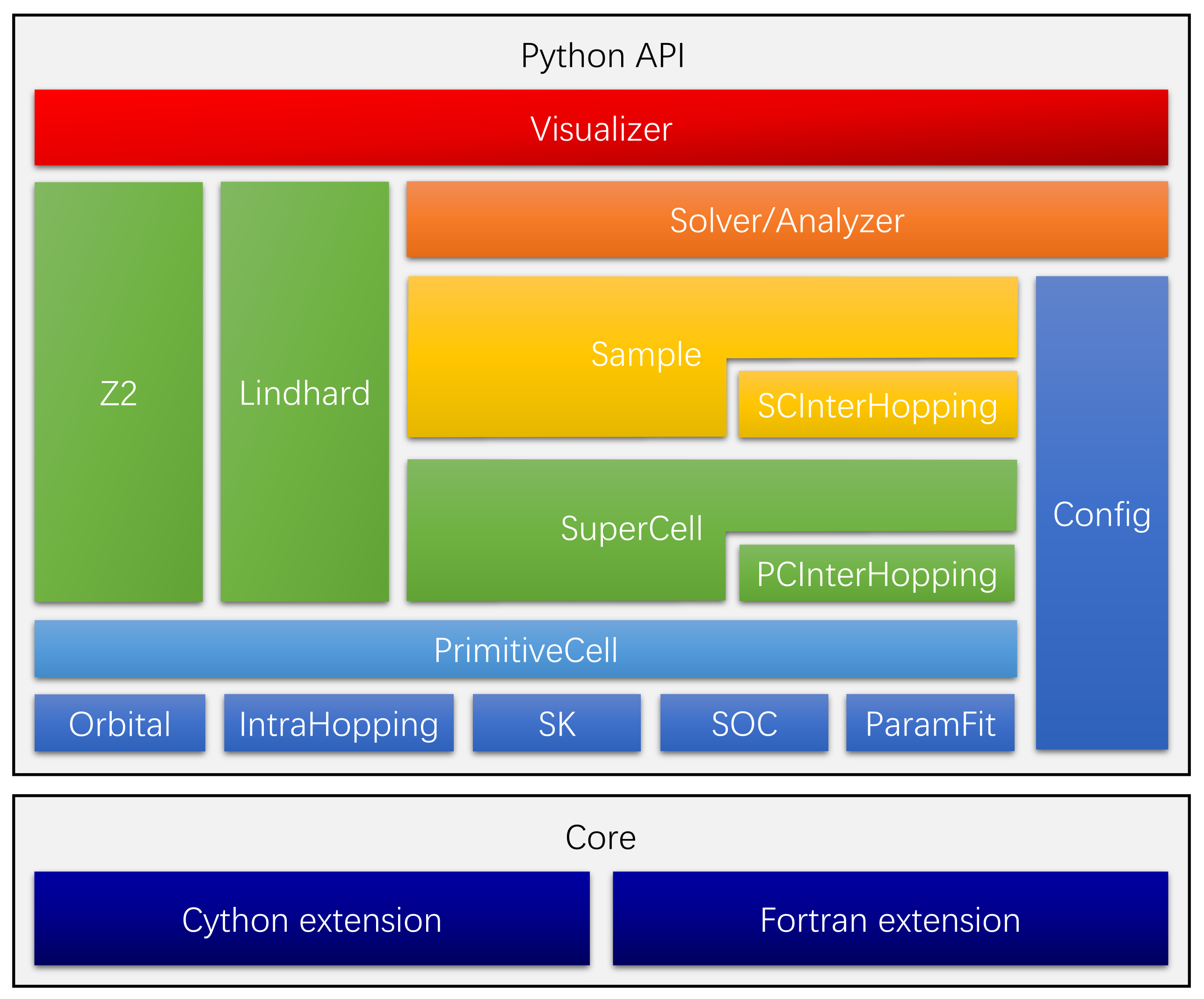
Figure 1: Program layout of TBPLaS. Components of the same level in the hierarchy share the same color.

3.2 PrimitiveCell

As aforementioned in section 3.1, the main purpose of PrimitiveCell class is to represent and solve tight-binding models of small and moderate size. It is also the building block for large and complex models. All calculations utilizing TBPLaS begin with creating the primitive cell. The user APIs of PrimitiveCell as well as many miscellaneous tools are summarized in Table 1. To create the primitive cell, one needs to provide the lattice vectors, which can be generated with the gen_lattice_vectors function or manually specifying their Cartesian coordinates. Then the orbitals and hopping terms are added to the primitive cell with the add_orbital and add_hopping functions, respectively. TBPLaS utilizes the conjugate relation to reduce the hopping terms, so only half of them are needed. There are also functions to extract, modify and remove existing orbitals and hopping terms in the cell, e.g., set_orbital/get_orbital/remove_orbitals and get_hopping/remove_hopping. Removing orbitals and hopping terms may leave dangling items in the cell. In that case, the trim function becomes useful. By default, the primitive cell is assumed to be periodic along all 3 directions. However, it can be made non-periodic along specific directions by removing hopping terms along that direction, as implemented in the apply_pbc function. As TBPLaS utilizes the lazy evaluation technique, the sync_array function is provided for synchronizing the array attributes after modifying the model. Once the primitive cell has been created, it can be visualized by the plot function and dumped by the print function. Geometric properties such as lattice area, volume and reciprocal lattice vectors, and electronic properties like band structure and DOS can be obtained with proper functions as listed in Table 1. The $\mathbf{k}$-points required for the evaluation of band structure and DOS can be generated with the gen_kpath and gen_kmesh functions, respectively.

TBPLaS ships with a collection of auxiliary tools for setting up the on-site energies and hopping terms. The SK class evaluates the hopping terms between atomic states up to $d$ orbitals according to the Slater-Koster formula. The SOC class evaluates the matrix element of intra-atom spin-orbital coupling term $\mathbf{L}\cdot\mathbf{S}$ in the direct product basis of $|l\rangle\otimes|s\rangle$. The ParamFit class is intended for fitting the on-site energies and hopping terms to reference data, which is typically from experiments or ab initio calculations.

For the user’s convenience, TBPLaS provides a model repository which offers the utilities to obtain the primitive cells of popular two-dimensional materials, as summarized in Table 1. The function make_antimonene returns the 3-orbital or 6-orbtial primitive cell of antimonene[78] depending on the inclusion of spin-orbital coupling. Diamond-shaped and rectangular primitive cells of graphene based on $p_{z}$ orbitals can be built with make_graphene_diamond and make_graphene_rect functions, respectively. A more complicated 8-band primitive cell based on $s$, $p_{x}$, $p_{y}$ and $p_{z}$ orbitals can be obtained with make_graphene_sp. The 4-orbital primitive cell of black phosphorus[79] can be obtained with make_black_phosphorus, while the 11-orbital models of transition metal dichalcogenides[80] are available with the make_tmdc function. The primitive cell can also be created from the output of Wannier90[81] package, namely seedname.win, seedname_centres.xyz and seedname_hr.dat, with the wan2pc function.

Starting from the simple primitive cell, more complex cells can be constructed through some common operations. A set of functions are provided for this purpose. extend_prim_cell replicates the primitive cell by given times. reshape_prim_cell reshapes the cell to new lattice vectors, while sprical_prim_cell shifts and rotates the cell with respect to c-axis, both of which are particularly useful for constructing hetero-structures. make_hetero_layer is a wrapper over reshape_prim_cell and produces one layer of the hetero-structure. Inter-cell hopping terms within a hetero-structure can be searched with the find_neighbors function and managed with the PCInterHopping class. Finally, all the layers and intercell hopping terms can be merged into one cell by the merge_prim_cell function. Note all these functions work at PrimitiveCell level, i.e., they either return a new primitive cell, or modify an existing one.

Table 1: User APIs of PrimitiveCell, SK, SOC, ParamFit, PCInterHopping classes and and miscellaneous tools.

Category	API	Purpose
PrimitiveCell	add_orbital	Add a new orbital
	set_orbital	Modify an existing orbital
	get_orbital	Retrieve an existing orbital
	remove_orbitals	Remove selected orbitals
	add_hopping	Add a new or modify an existing hopping term
	get_hopping	Retrieve an existing hopping term
	remove_hopping	Remove an existing hopping term
	trim	Remove dangling orbitals and hopping terms
	apply_pbc	Modify the boundary conditions
	sync_array	Synchronize the array attributes
	get_lattice_area	Calculate the area spanned by lattice vectors
	get_lattice_volume	Calculate the volume spanned by lattice vectors
	get_reciprocal_vectors	Calculate reciprocal lattice vectors
	calc_bands	Calculate band structure of the primitive cell
	calc_dos	Calculate DOS and LDOS of the primitive cell
	plot	Plot the primitive cell to the screen or file
	print	Print orbital and hopping terms
SK	eval	Evaluate hopping term with Slater-Koster formula
SOC	eval	Evaluate matrix element of $\mathbf{L}\cdot\mathbf{S}$ in direct product basis
ParamFit	fit	Fit on-site energies and hopping terms to reference data
PCInterHopping	add_hopping	Add a new inter-cell hopping term
Lattice and k-points	gen_lattice_vectors	Generate lattice vectors from lattice constants
	rotate_coord	Rotate Cartesian coordinates
	cart2frac	Convert coordinates from Cartesian to fractional
	frac2cart	Convert coordinates from fractional to Cartesian
	gen_kpath	Generate path connecting highly-symmetric $\mathbf{k}$-points
	gen_kmesh	Generate a mesh grid in the first Brillouin zone
Model repository	make_antimonene	Get the primitive cell of antimonene
	make_graphene_diamond	Get the diamond-shaped primitive cell of graphene
	make_graphene_rect	Get the rectangular primitive cell of graphene
	make_graphene_sp	Get the 8-band primitive cell of graphene
	make_black_phosphorus	Get the primitive cell of black phosphorus
	make_tmdc	Get the primitive cells of transition metal dichalcogenides
	wan2pc	Create primitive cell from the output of Wannier90
Modeling tools	extend_prim_cell	Replicate the primitive cell
	reshape_prim_cell	Reshape primitive cell to new lattice vectors
	spiral_prim_cell	Rotate and shift primitive cell
	make_hetero_layer	Produce one layer of hetero-structure
	find_neighbors	Find neighboring orbital pairs up to cutoff distance
	merge_prim_cell	Merge primitive cells and inter-cell hopping terms

3.3 Lindhard

The Lindhard class evaluates response properties, i.e., dynamic polarization, dielectric function and optical conductivity of primitive cell with the help of Lindhard function. The user APIs of this class is summarized in Table 2. To instantiate a Lindhard object, one needs to specify the primitive cell, energy range and resolution, dimension of $\mathbf{k}$-grid in the first Brillouin zone, system dimension, background dielectric constant and many other quantities. Since dynamic polarization and dielectric function are $\mathbf{q}$-dependent, three types of coordinate systems are provided to effectively represent the $\mathbf{q}$-points: Cartesian coordinate system in unit of $\mathrm{\AA}^{-1}$ or $\mathrm{nm}^{-1}$, fractional coordinate system in unit of reciprocal lattice vectors, and grid coordinate system in unit of dimension of $\mathbf{k}$-grid. Grid coordinate system is actually a variant of the fractional coordinate system. Conversion between coordinate systems can be achieved with the frac2cart and cart2frac functions.

Lindhard class offers two functions to calculate the dynamic polarization: calc_dyn_pol_regular and calc_dyn_pol_arbitrary. Both functions require an array of $\mathbb{q}$-points as input. The difference is that calc_dyn_pol_arbitrary accepts arbitrary $\mathbb{q}$-points, while calc_dyn_pol_regular requires that the $\mathbb{q}$-points should be on the uniform $\mathbb{k}$-grid in the first Brillouin zone. This is due to the term $\mathbb{k\textquoteright=k+q}$ that appears in the Lindhard function. For regular $\mathbb{q}$ on $\mathbb{k}$-grid, $\mathbb{k^{\prime}}$ is still on the same grid. However, this may not be true for arbitrary $\mathbb{q}$-points. So, calc_dyn_pol_arbitrary keeps two sets of energies and wave functions, for $\mathbb{k}$ and $\mathbb{k^{\prime}}$ grids respectively, although they may be equivalent via translational symmetry. On the contrary, calc_dyn_pol_regular utilizes translational symmetry and reuses energies and wave functions when possible. So, calc_dyn_pol_regular uses less computational resources, at the price that only regular $\mathbb{q}$-points on $\mathbb{k}$-grid can be taken as input. From the dynamic polarization, dielectric function can be obtained by calc_epsilon. Unlike dynamic polarization and dielectric function, the optical conductivity considered in TBPLaS does not depend on $\mathbb{q}$-points. So, it can be evaluated directly by calc_ac_cond.

Table 2: User APIs of Lindhard and Z2 classes.

Category	API	Purpose
Lindhard	calc_dyn_pol_regular	Calculate dynamic polarization for regular $\mathbf{q}$-points
	calc_dyn_pol_arbitrary	Calculate dynamic polarization for arbitrary $\mathbf{q}$-points
	calc_epsilon	Calculate dielectric function
	calc_ac_cond	Calculate optical conductivity
Z2	calc_phases	Calculate phases $\theta_{m}^{D}$
	reorder_phases	Reorder phases improve continuity and smoothness
	count_crossing	Count crossing number of phases against reference line

3.4 Z2

The Z2 class evaluates and analyzes the topological phases $\theta_{m}^{D}$ to yield the $\mathbb{Z}_{2}$ number. The APIs of this class are summarized in Table 2. To create a Z2 calculator, the primitive cell, as well as the number of occupied bands should be provided as input. The phases $\theta_{m}^{D}$ can be obtained as the function of $\mathbf{k}_{b}$ with the calc_phases function, which can then be plotted with scatter plot to count the crossing number against a reference line. If there are too many occupied states, it may be difficult to determine the crossing number with human eyes. The count_crossing function can count the crossings automatically, provided that the phases have been correctly reordered with the reorder_phases function. Anyway, the users are strongly recommended to cross-validate the crossing numbers from scatter plot and count_crossing, respectively. Finally, the $\mathbb{Z}_{2}$ number is determined as the remainder of crossing number divided by 2.

3.5 SuperCell, SCInterHopping and Sample

The tools discussed in section 3.2 are sufficiently enough to build complex models of small and moderate size. However, there are occasions where large models are essential, e.g., hetero-structures with twisted layers, quasi crystals, distorted structures, etc. In particular, TBPM calculations require large models for numerical stability. To build and manipulate large models efficiently, a new set of classes, namely SuperCell, SCInterHopping and Sample are provided. The APIs of these classes are summarized in Table 3.

The purpose of SuperCell class is to represent homogenous models that are formed by replicating the primitive cell. To create a supercell, the primitive cell, supercell dimension and boundary conditions are required. Vacancies can be added to the supercell upon creation, or through the add_vacancies and set_vacancies functions afterwards. Modifications to the hopping terms can be added by the add_hopping function. If the hopping terms are already included in the supercell, the original values will be overwritten. Otherwise, they will be added to the supercell as new terms. The supercell can be assgined with an orbital position modifier with the set_orb_pos_modifier function, which is a Python function modifying the orbital positions in-place. Dangling orbitals and hopping terms in the supercell can be removed by the trim function. Orbital positions, on-site energies, hopping terms and distances, as well as many properties of the supercell cell can be obtained with the get_xxx functions, as listed in Table 3. TBPLaS utilizes the conjugate relation to reduce the hopping terms, so only half of them are returned by get_hop and get_dr.

Heterogenous systems, e.g., slabs with adatoms or hetero-structures with multiple layers, are modelled as separate supercells and containers for inter-supercell hopping terms. The containers are created from the SCInterHopping class, with a bra supercell and a ket supercell, between which the hopping terms can be added by the add_hopping function. The SCInterHopping class also implements the get_hop and get_dr functions for extracting the hopping terms and distances, similar to the SuperCell class.

The Sample class is a unified interface to both homogenous and heterogenous systems. A sample may consist of single supercell, or multiple supercells and inter-supercell hopping containers. The on-site energies, orbital positions, hopping terms and distances are stored in the attributes of orb_eng, orb_pos, hop_i, hop_j, hop_v and dr, respectively, which are all numpy arrays. To reduce the memory usage, these attributes are filled only when needed with the initialization functions. Different kinds of perturbations, e.g., electric and magnetic fields, strain, can be specified by directly calling the API, or manipulating the array attributes directly. The reset_array function is provided to reset the array attributes of the sample, for removing the effects of perturbations. Band structure and DOS of the sample can be obtained with calc_bands and calc_dos respectively, similar to the PrimitiveCell class. Visualization is achieved through the plot function. Since the sample is typically large, its response properties are no longer accessible via the Lindhard function. On the contrary, TBPM is much more efficient for large samples. Since the Chebyshev polynomial decomposition of Hamiltonian requires its eigenvluates to be within [-1, 1], an API rescale_ham is provided for this purpose. Details on TBPM will be discussed in the next section.

Table 3: User APIs of SuperCell, SCInterHopping and Sample classes.

Category	API	Purpose
SuperCell	add_vacancies	Add a list of vacancies to the supercell
	set_vacancies	Reset the list of vacancies
	add_hopping	Add a modification to the hopping terms
	set_orb_pos_modifier	Assign an orbital position modifier to the supercell
	trim	Remove dangling orbitals and hopping terms
	sync_array	Synchronize the array attributes
	get_orb_pos	Get the Cartesian coordinates of orbitals
	get_orb_eng	Get the on-site energies
	get_hop	Get the hopping terms
	get_dr	Get the hopping distances
	get_lattice_area	Calculate the area spanned by lattice vectors
	get_lattice_volume	Calculate the volume spanned by lattice vectors
	get_reciprocal_vectors	Calculate reciprocal lattice vectors
SCInterHopping	add_hopping	Add a new inter-supercell hopping term
	get_hop	Get the hopping terms
	get_dr	Get the hopping distances
Sample	init_orb_eng	Initialize on-site energies on demand
	init_orb_pos	Initialize orbital positions on demand
	init_hop	Initialize hopping terms on demand
	init_dr	Initialize hopping distances on demand
	reset_array	Reset the array atributes
	rescale_ham	Rescale the Hamiltonian
	set_magnetic_field	Apply a perpendicular magnetic field
	calc_bands	Calculate band structure of the sample
	calc_dos	Calculate DOS and LDOS of the sample
	plot	Plot the sample to the screen or file

3.6 Config, Solver, Analyzer and Visualizer

TBPM in TBPLaS is implemented in the classes of Config, Solver and Analyzer. Config is a simple container class holding all the parameters that controls the calculation. So, it has no API but a few Python dictionaries as attributes. The Solver class propagates the wave function and evaluates the correlation functions, which are then analyzed by Analyzer class to produce the results, including DOS, LDOS, optical conductivity, electric conductivity, etc. The user APIs of Solver and Analyzer are summarized in Table 4. To create a solver or analyzer, one needs the sample and the configuration object. The APIs of Solver and Analyzer share a common naming convention, where calc_corr_xxx calculates the correlation function for property xxx and calc_xxx analyzes the correlation function to yield the final results. Some of the properties, such as LDOS from Green’s function and time-dependent wave function, can be obtained from Solver directly without further analysis.

The Visualizer class is a thin wrapper over matplotlib for quick visualization of the results from exact-diagonalization and TBPM. Generic data, e.g., response functions, can be plotted with the plot_xy function. There are also special functions to plot the band structure, DOS and topological phases. Quasi-eigenstates and time-dependent wave function can be plotted with the plot_wfc function. Although Visualizer is intended for quick visualization, it can be easily extended to produce figures of publication quality, according to the user’s needs.

Table 4: User APIs of Solver, Analyzer, Visualizer classes.

Category	API	Purpose
Solver	set_output	Prepare output directory and files
	save_config	Save configuration to file
	calc_corr_dos	Calculate correlation function of DOS
	calc_corr_ldos	Calculate correlation function of LDOS
	calc_corr_dyn_pol	Calculate correlation function of dynamical polarization
	calc_corr_ac_cond	Calculate correlation function of optical conductivity
	calc_corr_dc_cond	Calculate correlation function of electric conductivity
	calc_hall_mu	Calculate $\mu_{mn}$ required for the evaluation of Hall conductivity using Kubo-Bastin formula
	calc_quasi_eigenstates	Calculate quasi-eigenstates of given energies
	calc_ldos_haydock	Calculate LDOS using Green’s function
	calc_wfc_t	Calculate propagation of wave function from given initial state
Analyzer	calc_dos	Calculate DOS from its correlation function
	calc_ldos	Calculate LDOS from its correlation function
	calc_dyn_pol	Calculate dynamic polarization from its correlation function
	calc_epsilon	Calculate dielectric function from dynamic polarization
	calc_ac_cond	Calculate optical conductivity from its correlation function
	calc_dc_cond	Calculate electric conductivity from its correlation function
	calc_diff_coeff	Calculate diffusion coefficient from DC correlation function
	calc_hall_cond	Calculate Hall conductivity from $\mu_{mn}$
Visualizer	plot_xy	Plot generic data of y against x
	plot_bands	Plot band structure
	plot_dos	Plot DOS
	plot_phases	Plot phases $\theta_{m}^{D}$
	plot_wfc	Plot quasi-eigenstate or time-dependent wave function in real space

3.7 Parallelization

Tight-binding calculations can be time-consuming when the model is large, or when ultra-fine results are desired. For example, band structure, DOS, response properties from Lindhard function and topological phases from Z2 require exact diagonalization for a dense $\mathbf{k}$-grid in the first Brillouin zone, optionally followed by post-processing on an energy grid. TBPM calculations require large models and averaging over multiple samples to converge the results, while the time-propagation of each sample involves heavy matrix-vector multiplications. Consequently, dedicated parallelism that can exploit the modern hardware of computers are essential to promote the application of tight-binding techniques to millions or even billions of orbitals. However, the Global Interpreter Lock (GIL) of Python allows only one thread to run at one time, severely hinders the parallelization at thread level. Although the GIL can be bypassed with some tricks, thread-level parallelization is restricted to only one computational node. TBPLaS tackles these problems with a hybrid MPI+OpenMP parallelism. Tasks are firstly distributed over MPI processes that can run among multiple nodes. Since the processes are isolated mutually at operation system level and each keeps a local copy of the data, there is no need to worry about data conflicts and GIL. For the tasks assigned to each process, thread-level parallelism is implemented with OpenMP in the Cython and Fortran extensions. With a wise choice of the numbers of processes and threads, excellent scaling can be achieved with respect to the computational resources. Both MPI and OpenMP of the hybrid parallelism can be enabled or disabled separately, ensuring good flexibility.

3.7.1 Band structure and DOS

For calculating the band structure, $\mathbb{k}$-points are firstly distributed over MPI processes, with each process dealing with some of the $\mathbb{k}$-points. For each $\mathbb{k}$-point assigned to the process, the Hamiltonian matrix has to be built in serial, while the diagonalization is further parallelized with OpenMP in the NumPy and SciPy libraries, which call OpenBLAS or MKL under the hood. The evaluation of DOS consists of getting the eigenvalues for a dense $\mathbb{k}$-grid, and a summation over the eigenvalues to collect the contributions following Eq. (39). Getting the eigenvalues is parallelized in the same approach as the band structure. The summation is parallelized with respect to the $\mathbb{k}$-points over MPI processes. Local data on each process is then collected via the MPI_Allreduce call.

3.7.2 Response properties from Lindhard function

Evaluation of response properties using Lindhard function is similar to that of DOS, which also consists of getting the eigenvalues and eigenvectors and subsequent post-processing. However, the post-processing is much more expensive than DOS. Taking the optical conductivity for example, whose formula follows Eq. (60). To reuse the intermediate results, we define the following arrays

$$\Delta\epsilon(\mathbb{k},m,n)=\epsilon_{m\mathbb{k}}-\epsilon_{n\mathbb{k}}$$ (93)

and

$$P(\mathbb{k},m,n)=\frac{f_{m\mathbb{k}}-f_{n\mathbb{k}}}{\epsilon_{m\mathbb{k}}-\epsilon_{n\mathbb{k}}}\langle\psi_{n\mathbb{k}}|v_{\alpha}|\psi_{m\mathbb{k}}\rangle\langle\psi_{m\mathbb{k}}|v_{\beta}|\psi_{n\mathbb{k}}\rangle$$ (94)

The evaluation of $\Delta\epsilon$ and $P$ are firstly parallelized with respect to $\mathbb{k}$ over MPI processes. For each process, tasks are further parallelized with respect to $m$ over OpenMP threads. Once the arrays are ready, the optical conductivity can be calculated as

$$\sigma_{\alpha\beta}(\hbar\omega)=\frac{\mathrm{i}e^{2}\hbar}{N_{\mathbb{k}}\Omega_{c}}\sum_{\mathbb{k}}\sum_{m,n}\frac{P(\mathbb{k},m,n)}{\Delta\epsilon(\mathbb{k},m,n)-(\hbar\omega+\mathrm{i}\eta^{+})}$$ (95)

Typically, the response properties are evaluated on a discrete frequency grid $\{\omega_{i}\}$. We firstly distribute $\mathbb{k}$-points over MPI processes, then distribute the frequencies over OpenMP threads. Final results are collected by MPI calls, similar to the evaluation of DOS.

3.7.3 Z2

The evaluation of topological phases $\theta_{m}^{D}$ according to Eq. (92) can be done for each $\mathbf{k}_{b}$ individually. So, tasks are distributed among MPI process with respect to $\mathbf{k}_{b}$. For given $\mathbf{k}_{b}$, the $D(\mathbf{k}_{b})$ matrix is evaluated in serial mode by iterative matrix multiplication according to Eq. (90). Then it is diagonalized to yield the eigenvectors $\lambda_{m}^{D}$, from which the phases $\theta_{m}^{D}$ can be extracted. Finally the results are collected with MPI calls.

3.7.4 TBPM

The TBPM calculations follow a common procedure. Firstly, the time-dependent wave function is propagated from different initial conditions and correlation functions are evaluated at each time-step. Then the correlation functions are averaged and analyzed to yield the final results. The averaging and analysis are cheap and need no parallelization. The propagation of wave function, on the contrary, is much more expensive and must be parallelized. Fortunately, propagation from each initial condition is embarrassingly parallel task, i.e., it can be split into individual sub-tasks that do not exchange data mutually. So, the initial conditions are distributed among MPI processes. The propagation of wave function, according to Eq. (30), involves heavy matrix-vector multiplications. In TBPLaS the matrices are stored in Compressed Sparse Row (CSR) format, significantly reducing the memory cost. The multiplication, as well as many other matrix operations, are parallelized with respect to matrix elements among OpenMP threads. Averaging of correlation functions is also done by MPI calls.

4 Usage

In this section we demonstrate the installation and usages of TBPLaS. TBPLaS is released under the BSD license, which can be found at https://opensource.org/licenses/BSD-3-Clause. The source code is available at the home page www.tbplas.net. Detailed documentation and tutorials can also be found there.

4.1 Installation

4.1.1 Prerequisites

To install and run TBPLaS, a Unix-like operating system is required. You need both C and Fortran compilers, as well as vendor-provided math libraries if they are available. For Intel^® CPUs, it is better to use Intel compilers and Math Kernel Library (MKL). If Intel toolchain is not available, the GNU Compiler Collection (GCC) is another choice. In that case, the built-in math library will be enabled automatically.

TBPLaS requires a Python3 environment (interpreter and development files), and the packages of NumPy, SciPy, Matplotlib, Cython, Setuptools as mandatory dependencies. Optionally, the LAMMPS interface requires the ASE package. If MPI+OpenMP hybrid parallelism is to be enabled, the MPI4PY package and an MPI implementation, e.g., Open MPI or MPICH, become essential. Most of the packages can be installed via the pip command, or manually from the source code.

4.1.2 Installation

The configuration of compilation is stored in setup.cfg in the top directory of the source code of TBPLaS. Examples of this file can be found in the config directory. You should adjust it according to your computer’s hardware and software settings. Here is an example utilizing Intel compilers and MKL

⬇

1[config_cc]

2compiler = intelem

3

4[config_fc]

5fcompiler = intelem

6arch = -xHost

7opt = -qopenmp -O3 -ipo -heap-arrays 32

8f90flags = -fpp -DMKL -mkl=parallel

9

10[build_ext]

11include_dirs = /software/intel/parallelstudio/2019/compilers_and_libraries/linux/mkl/include

12library_dirs = /software/intel/parallelstudio/2019/compilers_and_libraries/linux/mkl/lib/intel64

13libraries = mkl_rt iomp5 pthread m dl

The config_cc and config_fc sections contain the settings of C and Fortran compilers, while the libraries are configured in build_ext. It is important that OpenMP should be enabled by adding proper flags to config_fc and build_ext, e.g., -qopenmp in opt and iomp5 in libraries for Intel compilers. Here is another example utilizing GCC and the built-in math library

⬇

1[config_cc]

2compiler = unix

3

4[config_fc]

5fcompiler = gfortran

6arch = -march=native

7opt = -fopenmp -O3 -mtune=native

8f90flags = -fno-second-underscore -cpp

9

10[build_ext]

11libraries = gomp

where the OpenMP flags become -fopenmp and gomp.

Once setup.cfg has been properly configured, TBPLaS can be compiled with python setup.py build. If everything goes well, a new build directory will be created, which contains the Cython and Fortran extensions. The installation into default path is done by python setup.py install. After that, invoke the Python interpreter and try import tbplas. If no error occurs, then the installation of TBPLaS is successful.

4.2 Overview of the workflow

The workflow of common usages of TBPLaS is summarized in Fig. 2. Tight-binding models can be created at either PrimitiveCell or Sample level, depending on the model size and purpose. PrimitiveCell is recommended for models of small and moderate size, and is essential for evaluating response functions utilizing the Lindhard function or topological variants with the Z2 class. On the contrary, Sample is for extra-large models that may consist of millions or trillions of orbitals. Also, TBPM calculations require the model to be an instance of the Sample class. For a detailed comparison of PrimitiveCell and Sample, refer to section 3.

Generally, all calculations utilizing TBPLaS begin with creating the primitive cell, which involves creating an empty cell from the lattice vectors, adding orbitals and adding hoping terms. Complex models, e.g., that with arbitrary shape and boundary conditions, vacancies, impurities and hetero-structures can be constructed from the simple primitive cell with the Python-based modeling tools, as discussed in section 3.2. Band structure and DOS of the primitive cell can be obtained via exact diagonalization with the calc_bands and calc_dos functions, respectively. Response functions such dynamic polarization, dielectric function and optical conductivity, need an additional step of creating a Lindhard calculator, followed by calling the corresponding functions. Similar procedure applies to the topological properties, where a Z2 calculator should be created and utilized.

To build a sample, the user needs to construct a supercell with the Cython-based modeling tools. Heterogenous systems are modeled as separate supercells plus containers for inter-supercell hopping terms. The sample is then formed by assembling the supercells and containers. Band structure and DOS of the sample can be obtained via exact diagonalization in the same approach as the primitive cell. However, these calculations may be extremely slow due to the large size of the model. In that case, TBPM is recommended. The user needs to setup the parameters using the Config class, and create a solver and an analyzer from Solver and Analyzer classes, respectively. Then evaluate and analyze the correlation functions to yield the DOS, response functions, quasieigenstates, etc. Finally, the results can be visualized using the Visualizer class, or the matplotlib library directly.

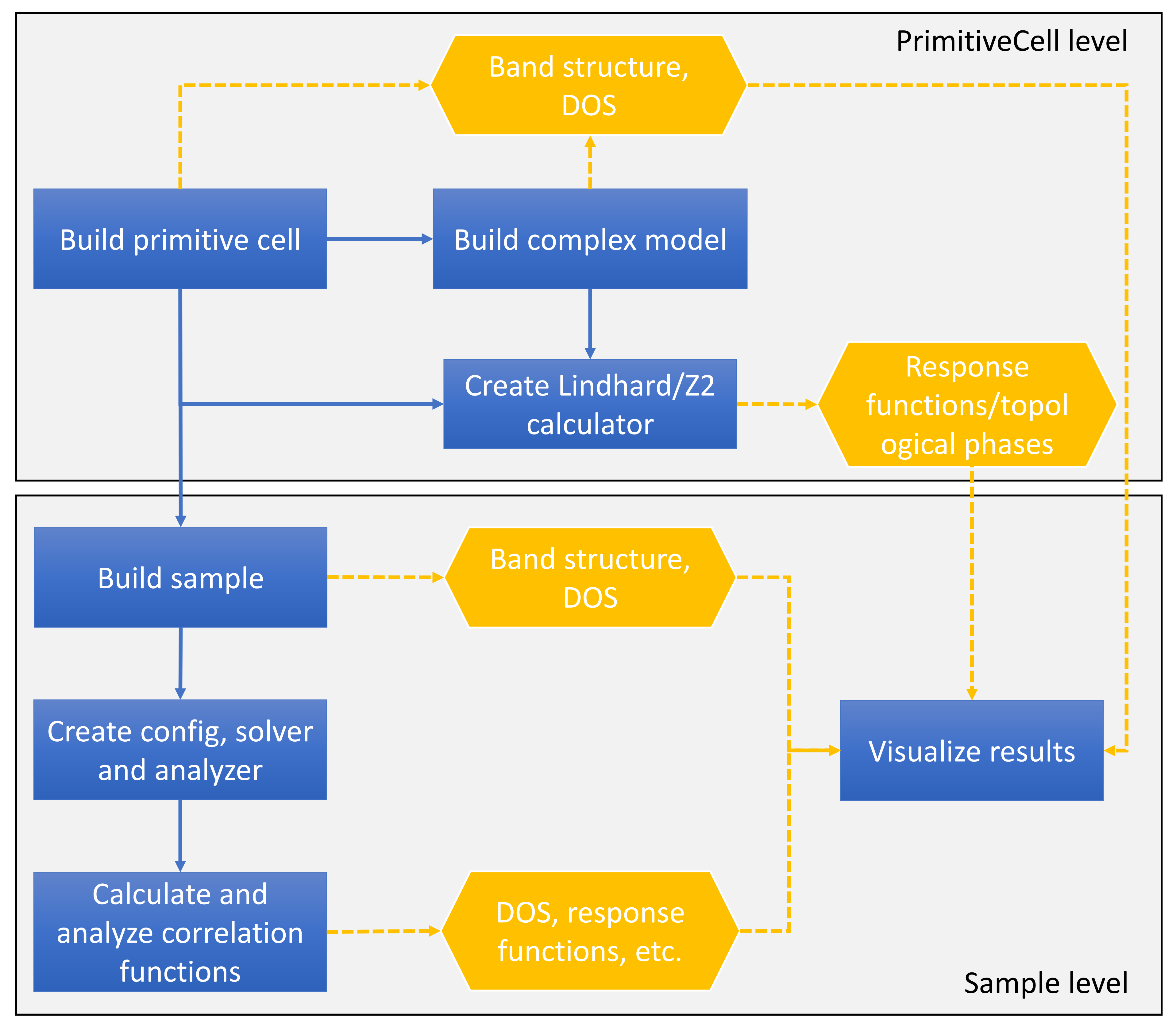
Figure 2: Workflow of common usages of TBPLaS. Blue rectangles and orange hexagons denote the main steps and outputs, respectively.

4.3 Building the primitive cell

In this section we show how to build the primitive cell taking monolayer graphene as the example. Monolayer graphene has lattice constants of $a=b=2.46\;\mathrm{\AA}$ and $\alpha=\beta=90^{\circ}$. The lattice angle $\gamma$ can be either $60^{\circ}$ or $120^{\circ}$, depending on the choice of lattice vectors. Also, we need to specify an arbitrary cell length $c$ since TBPLaS internally treats all models as three-dimensional. We will take $\gamma=60^{\circ}$ and $c=10\;\mathrm{\AA}$ . First of all, we need to invoke the Python interpreter and import all necessary packages

⬇

1import math

2import numpy as np

3import tbplas as tb

Then we generate the lattice vectors from the lattice constants with the gen_lattice_vectors function

⬇

1vectors = tb.gen_lattice_vectors(a=2.46, b=2.46, c=10.0, gamma=60)

The function accepts six arguments, namely a, b, c, alpha, beta, and gamma. The default value for alpha and beta is 90 degrees, if not specified. The return value vectors is a $3\times 3$ array containing the Cartesian coordinates of the lattice vectors. Alternatively, we can create the lattice vectors from their Cartesian coordinates directly

⬇

1a = 2.46

2c = 10.0

3a_half = a * 0.5

4sqrt3 = math.sqrt(3)

5

6vectors = np.array([

7 [a, 0, 0,],

8 [a_half, sqrt3*a_half, 0],

9 [0, 0, c]

10])

From the lattice vectors, we can create an empty primitive cell by

⬇

1prim_cell = tb.PrimitiveCell(vectors, unit=tb.ANG)

where the argument unit specifies that the lattice vectors are in Angstroms.

As we choose $\gamma=60^{\circ}$, the two carbon atoms are then located at $\tau_{0}=\mathbf{0}$ and $\tau_{1}=\frac{1}{3}\mathbf{a}_{1}+\frac{1}{3}\mathbf{a}_{2}$, as shown in Fig. 3 (a). In the simplest 2-band model of graphene, each carbon atom carries one $2p_{z}$ orbital. We can add the orbitals with the add_orbital function

⬇

1prim_cell.add_orbital([0., 0.], energy=0.0, label="pz")

2prim_cell.add_orbital([1./3, 1./3], energy=0.0, label="pz")

The first argument gives the position of the orbital, while energy specifies the on-site energy, which is assumed to be 0 eV if not specified. In absence of strain or external fields, the two orbitals have equal on-site energies. The argument label is a tag to denote the orbital. In addition to fractional coordinates, the orbitals can also be added using Cartesian coordinates by the add_orbital_cart function

⬇

1prim_cell.add_orbital_cart([0., 0.], unit=tb.ANG, energy=0.0, label="pz")

2prim_cell.add_orbital_cart([1.23, 0.71014083], unit=tb.ANG, energy=0.0, label="pz")

Here we use the argument unit to specify the unit of Cartesian coordinates.

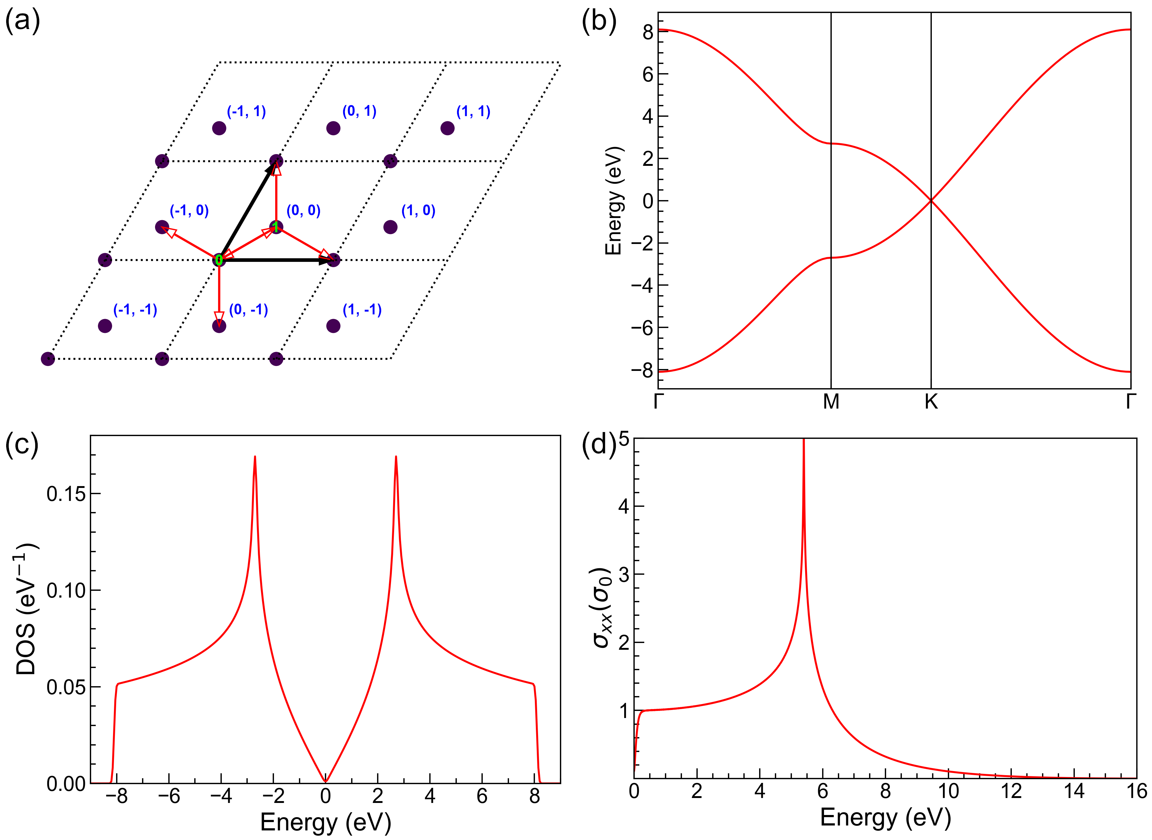
Figure 3: (a) Schematic plot of the primitive cell of monolayer graphene. Orbitals are shown as filled circles and numbered in green texts, while cells are indicated with dashed diamonds and numbered in blue texts. Thick black arrows denote the lattice vectors. (b) Band structure, (c) DOS and (d) Optical conductivity of monolayer graphene. The optical conductivity is in the unit of $\sigma_{0}=\frac{e^{2}}{4\hbar}$.

When all the orbitals have been added to the primitive cell, we can proceed with adding the hopping terms, which are defined as

$$t_{ij}(\mathbf{R})=\langle\phi_{i\mathbf{0}}|\hat{h}_{0}|\phi_{j\mathbf{R}}\rangle$$ (96)

where $\mathbf{R}$ is the index of neighbouring cell, $i$ and $j$ are orbital indices, respectively. The hopping terms of monolayer graphene in the nearest approximation are

• $\mathbf{R}=(0,0),i=0,j=1$

• $\mathbf{R}=(0,0),i=1,j=0$

• $\mathbf{R}=(1,0),i=1,j=0$

• $\mathbf{R}=(-1,0),i=0,j=1$

• $\mathbf{R}=(0,1),i=1,j=0$

• $\mathbf{R}=(0,-1),i=0,j=1$

With the conjugate relation $t_{ij}^{\phantom{*}}(\mathbf{R})=t_{ji}^{*}(-\mathbf{R})$, the hopping terms can be reduced to

• $\mathbf{R}=(0,0),i=0,j=1$

• $\mathbf{R}=(1,0),i=1,j=0$

• $\mathbf{R}=(0,1),i=1,j=0$

TBPLaS takes the conjugate relation into consideration. So, we need only to add the reduced set of hopping terms. This can be done with the add_hopping function

⬇

1prim_cell.add_hopping(rn=[0, 0], orb_i=0, orb_j=1, energy=-2.7)

2prim_cell.add_hopping(rn=[1, 0], orb_i=1, orb_j=0, energy=-2.7)

3prim_cell.add_hopping(rn=[0, 1], orb_i=1, orb_j=0, energy=-2.7)

The argument rn specifies the index of neighbouring cell, while orb_i and orb_j give the indices of orbitals of the hopping term. energy is the hopping integral, which should be a complex number in general cases.

Now we have successfully built the primitive cell. We can visualize it with the plot function:

⬇

1prim_cell.plot()

The output is shown in Fig. 3(a), with orbitals shown as filled circles and hopping terms as arrows. We can also print the details of the model with the print function:

⬇

1prim_cell.print()

The output is as follows

⬇

1Lattice vectors (nm):

2 0.24600 0.00000 0.00000

3 0.12300 0.21304 0.00000

4 0.00000 0.00000 1.00000

5Orbitals:

6 0.00000 0.00000 0.00000 0.0

7 0.33333 0.33333 0.00000 0.0

8Hopping terms:

9 (0, 0, 0) (0, 1) -2.7

10 (1, 0, 0) (1, 0) -2.7

11 (0, 1, 0) (1, 0) -2.7

4.4 Properties of primitive cell

In this section we show how to calculate the band structure, DOS and response functions of the graphene primitive cell that created in previous section. First of all, we need to generate a k-path of $\mathrm{\Gamma}\rightarrow\mathrm{M}\rightarrow\mathrm{K}\rightarrow\mathrm{\Gamma}$ with the gen_kpath function

⬇

1k_points = np.array([

2 [0.0, 0.0, 0.0],

3 [1./2, 0.0, 0.0],

4 [2./3, 1./3, 0.0],

5 [0.0, 0.0, 0.0],

6])

7k_label = ["$\Gamma$", "M", "K", "$\Gamma$"]

8k_path, k_idx = tb.gen_kpath(k_points, [40, 40, 40])

In this example, we interpolate with 40 intermediate $\mathbf{k}$-points along each segment of the $\mathbf{k}$-path. gen_kpath returns two arrays, with k_path containing the coordinates of $\mathbf{k}$-points and k_idx containing the indices of highly-symmetric $\mathbf{k}$-points in k_path. Then we solve the band structure with the calc_bands function

⬇

1k_len, bands = prim_cell.calc_bands(k_path)

Here k_len is the length of $\mathbf{k}$-path, while bands is a $N_{k}\times N_{b}$ matrix containing the energies. The band structure can be plotted with matplotlib

⬇

1num_bands = bands.shape[1]

2for i in range(num_bands):

3 plt.plot(k_len, bands[:, i], color="r", linewidth=1.2)

4for idx in k_idx:

5 plt.axvline(k_len[idx], color="k", linewidth=0.8)

6plt.xlim((0, np.amax(k_len)))

7plt.xticks(k_len[k_idx], k_label)

8plt.ylabel("Energy (eV)")

9plt.tight_layout()

10plt.show()

Or alternatively, using the Visualizer class:

⬇

1vis = tb.Visualizer()

2vis.plot_bands(k_len, bands, k_idx, k_label)

The output is shown in Fig. 3(b). The Dirac cone at $\mathrm{K}$-point is perfectly reproduced.

To calculate the DOS, we need to sample the first Brillouin zone with a dense $\mathbf{k}$-grid, e.g., $240\times 240\times 1$

⬇

1k_mesh = tb.gen_kmesh((240, 240, 1))

where k_mesh contains the coordinates of $\mathbf{k}$-points on the grid. Then we evaluate and visualize the DOS as

⬇

1energies, dos = prim_cell.calc_dos(k_mesh, e_min=-9, e_max=9)

2vis.plot_dos(energies, dos)

where energies is a uniform energy grid whose lower and upper bounds are controlled by the arguments e_min and e_max. dos is an array containing the DOS values at the grid points in energies. The output is shown in Fig. 3(c).

The evaluation of response functions requires a Lindhard calculator, which can be created by

⬇

1lind = tb.Lindhard(cell=prim_cell, energy_max=20, energy_step=2000, kmesh_size=(4096, 4096, 1), mu=0.0, temperature=300.0, g_s=2, back_epsilon=1.0)

The argument cell assigns the primitive cell to the calculator. energy_max and energy_step define a uniform energy grid on which response functions will be evaluated. kmesh_size specifies the size of $\mathbf{k}$-grid in the first Brillouin zone. As monolayer graphene is semi-metallic, we need a very dense $\mathbf{k}$-grid in order to converge the response functions. mu, temperature and g_s are the chemical potential, temperature and spin degeneracy of the system, while back_epsilon is the background dielectic constant, respectively. The xx component of optical conductivity, namely $\sigma_{xx}$, can be evaluated with the calc_ac_cond function

⬇

1omegas, ac_cond = lind.calc_ac_cond(component="xx")

where omegas is the energy grid and ac_cond is the optical conductivity. The results can be visualized using the Visualizer class

⬇

1ac_cond *= 4

2vis = tb.Visualizer()

3vis.plot_xy(omegas, ac_cond.real, x_label="Energy (eV)", y_label="$\sigma_{xx} (\sigma_0)$")

The output is shown in Fig. 3(d), in the unit of $\sigma_{0}=\frac{e^{2}}{4\hbar}$.

4.5 Building the sample

In this section we show how to construct a sample by making a graphene model with $20\times 20\times 1$ primitive cells. To build the sample, we need to create the supercell first

⬇

1super_cell = tb.SuperCell(prim_cell, dim=(20, 20, 1), pbc=(True, True, False))

The SuperCell class is similar to the functions of extend_prim_cell and apply_pbc, where the dimension and periodic boundary conditions are set up at the same time. The sample is formed by gluing the supercells and inter-hopping terms altogether with the Sample class. In our case the sample consists of only one supercell. So it can be created and visualized by

⬇

1sample = tb.Sample(super_cell)

2sample.plot(with_orbitals=False, with_cells=False, hop_as_arrows=False)

where some options are switched for boosting the plot. The output is shown in Fig. 4(a).

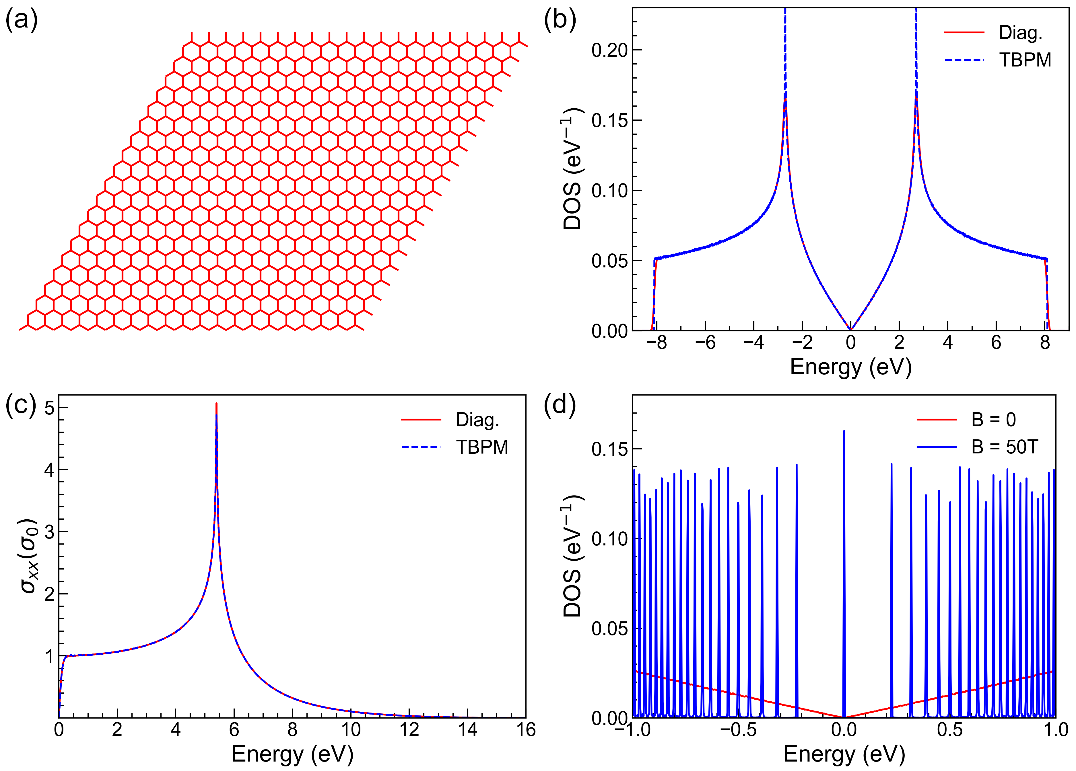
Figure 4: (a) Plot of the $20\times 20\times 1$ graphene sample. (b) DOS of graphene from exact-diagonalization and TBPM. (c) Optical conductivity of graphene from Lindhard function and TBPM. (d) DOS of graphene under zero and 50 Tesla magnetic fields.

4.6 Properties of sample

The Sample class supports the evaluation of band structure and DOS via exact-diagonalization with the calc_bands and calc_dos functions, similar to the PrimitiveCell class. Taking the DOS as an example, in section 4.4 we have sampled the first Brillouin zone with a $\mathbf{k}$-grid of $240\times 240\times 1$. Now that we have a much larger sample, the dimension of $\mathbf{k}$-grid can be reduced to $12\times 12\times 1$ accordingly

⬇

1k_mesh = tb.gen_kmesh((12, 12, 1))

2energies, dos = sample.calc_dos(k_mesh, e_min=-9, e_max=9)

3vis.plot_dos(energies, dos)

The output is shown in Fig. 4(b), which is consistent with Fig. 3(c).

Exact diagonalization-based techniques are not feasible for large models as the computational costs scale cubically with the model size. On the contrary, TBPM involves only matrix-vector multiplication, and is less demanding on computational resources. Therefore, TBPM is particularly suitable for large models with millions of orbitals or more. Current capabilities of TBPM in TBPLaS are summarized in section 3.6. We demonstrate the usage of TBPM to evaluate the DOS and optical conductivity of a graphene sample with $4096\times 4096\times 1$ primitive cells, i.e., 33,554,432 orbitals. We begin with creating the sample

⬇

1super_cell = tb.SuperCell(prim_cell, dim=(4096, 4096, 1), pbc=(True, True, False))

2sample = tb.Sample(super_cell)

3sample.rescale_ham(9.0)

Since the model is extremely large, we will not visualize it as in other examples. In TBPM the time evolution and Fermi-Dirac operators are expanded in Chebyshev polynomials, which requires the eigenvalues of the Hamiltonian to be within $[-1,1]$. So, we need to rescale the Hamiltonian with the rescale_ham function. The scaling factor can be specified as an argument. If not provided, a reasonable default value will be estimated from the Hamiltonian. Then we set up the parameters of TBPM in an instance of the Config class

⬇

1config = tb.Config()

2config.generic["nr_random_samples"] = 4

3config.generic["nr_time_steps"] = 4096

Here we set two parameters: nr_random_samples and nr_time_steps. nr_random_samples specifies that we are going to consider 4 random initial wave functions for the propagation, while nr_time_steps indicates the number of steps to propagate. The time step for the propagation is $\pi/f$ (in unit of $\hbar/eV$), with $f$ being the scaling factor of Hamiltonian in eV. Now we create a pair of solver and analyzer by

⬇

1solver = tb.Solver(sample, config)

2analyzer = tb.Analyzer(sample, config)

Then we calculate and analyze the correlation function to get DOS

⬇

1corr_dos = solver.calc_corr_dos()

2energies, dos = analyzer.calc_dos(corr_dos)

3vis = tb.Visualizer()

4vis.plot_dos(energies, dos)

Here the correlation function corr_dos is obtained with the calc_corr_dos function, and then analyzed by the calc_dos function to yield the energy grid energies and DOS values dos. The result is shown in Fig. 4(b), consistent with the results from exact-diagonalization.

The calculation of optical conductivity is similar to DOS

⬇

1config.generic["correct_spin"] = True

2corr_ac_cond = solver.calc_corr_ac_cond()

3omegas, ac_cond = analyzer.calc_ac_cond(corr_ac_cond)

4ac_cond *= 4

5vis.plot_xy(omegas, ac_cond[0].real, x_label="Energy (eV)", y_label="$\sigma_{xx} (\sigma_0)$")

Note that we set the spin-degeneracy of the model to 2 by setting the correct_spin argument to True, for consistency with the example in section 4.4. The optical conductivity is shown in Fig. 4(c), which matches perfectly with the results from Lindhard function.

4.7 Advanced modeling

In this section, we demonstrate how to construct complex models, including hetero structure, quasicrystal and fractal. For the hetero structure, we are going to take the twisted bilayer graphene as an example, while for the fractal we will consider the Sierpiński carpet.

4.7.1 Hetero-structure

The workflow of constructing hetero structures is shown in Fig. 5(a). First of all, we determine the twisting angle and lattice vectors of the hetero-structure. Then we build the primitive cells of each layer, shift the twisted layer along $z$-axis by the interlayer distance and rotate it by the twisting angle. After that, we reshape the primitive cells to the lattice vectors of the hetero-structure to yield the layers, as depicted in Fig. 5(b). When all the layers are ready, we merge them into one cell and add the intralayer and interlayer hopping terms up to a given cutoff distance. For the visualization of Moiré pattern, we also need to build a sample from the merged cell.

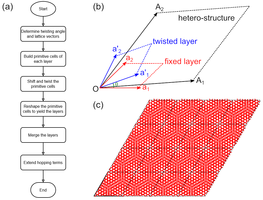
Figure 5: (a) Workflow of constructing hetero-structure. (b) Schematic plot of lattice vectors of fixed ($\mathbf{a}_{1}$, $\mathbf{a}_{2}$) and twisted ($\mathbf{a}_{1}^{\prime}$, $\mathbf{a}_{2}^{\prime}$) primitive cells and the hetero-structure ($\mathbf{A}_{1}$, $\mathbf{A}_{2}$), as well as the twisting angle $\theta$. (c) Twisted bilayer graphene sample with $4\times 4\times 1$ merged cells of $i=5$.

Before constructing the model, we need to import the required packages and define some necessary functions. The packages are imported by

⬇

1import math

2import numpy as np

3from numpy.linalg import norm

4import tbplas as tb

The twisting angle and lattice vectors are determined following the formulation in Ref. [82]

$$\theta_{i} =\arccos\frac{3i^{2}+3i+1/2}{3i^{2}+3i+1},$$ (97)

$$\mathbf{A}_{1} =i\cdot\mathbf{a}_{1}+(i+1)\cdot\mathbf{a}_{2},$$ (98)

$$\mathbf{A}_{2} =-(i+1)\cdot\mathbf{a}_{1}+(2i+1)\cdot\mathbf{a}_{2},$$ (99)

where $\mathbf{a}_{1}$ and $\mathbf{a}_{2}$ are the lattice vectors of the primitive cell of fixed layer and $i$ is the index of hetero-structure. We define the following functions accordingly

⬇

1def calc_twist_angle(i):

2 cos_ang = (3 * i**2 + 3 * i + 0.5) / (3 * i**2 + 3 * i + 1)

3 return math.acos(cos_ang)

4

5

6def calc_hetero_lattice(i, prim_cell_fixed):

7 hetero_lattice = np.array([[i, i + 1, 0],

8 [-(i + 1), 2 * i + 1, 0],

9 [0, 0, 1]])

10 hetero_lattice = tb.frac2cart(prim_cell_fixed.lat_vec, hetero_lattice)

11 return hetero_lattice

calc_twist_angle returns the twisting angle in radians, while calc_hetero_lattice returns the Cartesian coordinates of lattce vectors in nm. After merging the layers, we need to add the interlayer hopping terms. Meanwhile, the intralayer hoppings terms should also be extended in the same approach. We define the extend_hop function to achieve these goals

⬇

1def extend_hop(prim_cell, max_distance=0.75):

2 neighbors = tb.find_neighbors(prim_cell, a_max=1, b_max=1,

3 max_distance=max_distance)

4 for term in neighbors:

5 i, j = term.pair

6 prim_cell.add_hopping(term.rn, i, j, calc_hop(term.rij))

Here in line 2 we call the find_neighbors function to get the neighboring orbital pairs up to the cutoff distance max_distance. Then the hopping terms are evaluated according to the displacement vector rij with the calc_hop function and added to the primitive cell. The calc_hop function is defined according to the formulation in Ref. [83]

⬇

1def calc_hop(rij):

2 a0 = 0.1418

3 a1 = 0.3349

4 r_c = 0.6140

5 l_c = 0.0265

6 gamma0 = 2.7

7 gamma1 = 0.48

8 decay = 22.18

9 q_pi = decay * a0

10 q_sigma = decay * a1

11 dr = norm(rij).item()

12 n = rij.item(2) / dr

13 v_pp_pi = - gamma0 * math.exp(q_pi * (1 - dr / a0))

14 v_pp_sigma = gamma1 * math.exp(q_sigma * (1 - dr / a1))

15 fc = 1 / (1 + math.exp((dr - r_c) / l_c))

16 hop = (n**2 * v_pp_sigma + (1 - n**2) * v_pp_pi) * fc

17 return hop

With all the functions ready, we proceed to build the hetero-structure. In line 2-4 we evaluate the twisting angle of bilayer graphene for $i=5$. Then we construct the primitive cells of the fixed and twisted layers with the make_graphene_diamond function. The fixed primitive cell is located at $z=0$ and does not need rotation or shifting. On the other hand, the twisted primitive cell needs to be rotated counter-clockwise by the twisting angle and shifted towards $+z$ by 0.3349 nm, which is done with the spiral_prim_cell function. After that, we reshape the primitive cells to the lattice vectors of hetero-structure with the make_hetero_layer function, which is a wrapper to coordinate conversion and reshape_prim_cell. Then the layers are merged with merge_prim_cell and the hopping terms are extended with extend_hop using a cutoff distance of 0.75 nm. Finally, a sample with $4\times 4\times 1$ merged cells is created and plotted, with the hopping terms below 0.3 eV hidden for clarity. The output is shown in Fig. 5 (c), where the Moiré pattern can be clearly observed.

⬇

1def main():

2 # Evaluate twisting angle

3 i = 5

4 angle = calc_twist_angle(i)

5

6 # Prepare primitive cells of fixed and twisted layer

7 prim_cell_fixed = tb.make_graphene_diamond()

8 prim_cell_twisted = tb.make_graphene_diamond()

9

10 # Shift and rotate the twisted layer

11 tb.spiral_prim_cell(prim_cell_twisted, angle=angle, shift=0.3349)

12

13 # Reshape primitive cells to the lattice vectors of hetero-structure

14 hetero_lattice = calc_hetero_lattice(i, prim_cell_fixed)

15 layer_fixed = tb.make_hetero_layer(prim_cell_fixed, hetero_lattice)

16 layer_twisted = tb.make_hetero_layer(prim_cell_twisted, hetero_lattice)

17

18 # Merge layers

19 merged_cell = tb.merge_prim_cell(layer_fixed, layer_twisted)

20

21 # Extend hopping terms

22 extend_hop(merged_cell, max_distance=0.75)

23

24 # Visualize Moire pattern

25 sample = tb.Sample(tb.SuperCell(merged_cell, dim=(4, 4, 1), pbc=(True, True, False)))

26 sample.plot(with_orbitals=False, hop_as_arrows=False, hop_eng_cutoff=0.3)

27

28

29if __name__ == "__main__":

30 main()

4.7.2 Quasicrystal

Here we consider the construction of hetero structure-based quasicrystal, in which we also need to shift, twist, reshape and merge the cells. Taking bilayer graphene quasicrystal as an example, a quasicrystal with 12-fold symmtery is formed by twisting one layer by $30^{\circ}$ with respect to the center of $\mathbf{c}=\frac{2}{3}\mathbf{a}_{1}+\frac{2}{3}\mathbf{a}_{2}$, where $\mathbf{a}_{1}$ and $\mathbf{a}_{2}$ are the lattice vectors of the primitive cell of fixed layer. We begin with defining the geometric parameters

⬇

1angle = 30 / 180 * math.pi

2center = (2./3, 2./3, 0)

3radius = 3.0

4shift = 0.3349

5dim = (33, 33, 1)

Here angle is the twisting angle and center is the fractional coordinate of twisting center. The radius of the quasicrystal is controlled by radius, while shift specifies the interlayer distance. We need a large cell to hold the quasicrystal, whose dimension is given in dim. After introducing the parameters, we build the fixed and twisted layers by

⬇

1prim_cell = tb.make_graphene_diamond()

2layer_fixed = tb.extend_prim_cell(prim_cell, dim=dim)

3layer_twisted = tb.extend_prim_cell(prim_cell, dim=dim)

Then we shift and rotate the twisted layer with respect to the center and reshape it to the lattice vectors of fixed layer

⬇

1# Get the Cartesian coordinate of twisting center

2center = np.array([dim[0]//2, dim[1]//2, 0]) + center

3center = np.matmul(center, prim_cell.lat_vec)

4

5# Twist, shift and reshape top layer

6tb.spiral_prim_cell(layer_twisted, angle=angle, center=center, shift=shift)

7conv_mat = np.matmul(layer_fixed.lat_vec, np.linalg.inv(layer_twisted.lat_vec))

8layer_twisted = tb.reshape_prim_cell(layer_twisted, conv_mat)

Since we have extended the primitive cell by $33\times 33\times 1$ times, and we want the quasicrystal to be located in the center of the cell, we need to convert the coordinate of twisting center in line 2-3. The twisting operation is done by the spiral_prim_cell function, where the Cartesian coordinate of the center is given in the center argument. The fixed and twisted layers have the same lattice vectors after reshaping, so we can merge them safely

⬇

1# Merge bottom and top layers

2final_cell = tb.merge_prim_cell(layer_twisted, layer_fixed)

Then we remove unnecessary orbitals to produce a round quasicrystal with finite radius. This is done by a loop over orbital positions to collect the indices of unnecessary orbitals, and function calls to remove_orbitals and trim functions

⬇

1# Remove unnecessary orbitals

2idx_remove = []

3orb_pos = final_cell.orb_pos_nm

4for i, pos in enumerate(orb_pos):

5 if np.linalg.norm(pos[:2] - center[:2]) > radius:

6 idx_remove.append(i)

7final_cell.remove_orbitals(idx_remove)

8

9# Remove dangling orbitals

10final_cell.trim()

Finally, we extend the hoppings and visualize the quasicrystal

⬇

1extend_hop(final_cell)

2final_cell.plot(with_cells=False, with_orbitals=False, hop_as_arrows=False, hop_eng_cutoff=0.3)

The output is shown in Fig. 6.

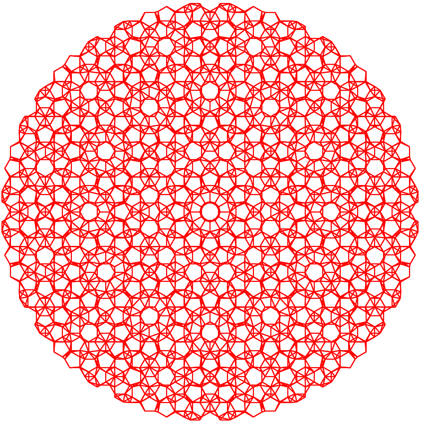
Figure 6: Plot of the quasicrystal formed from the incommensurate $30^{\circ}$ twisted bilayer graphene with a radius of 3 nm.

4.7.3 Fractal

Generally, fractals can be constructed in two approaches, namely bottom-up and top-down, as demonstrated in Fig. 7. The bottom-up approach builds the fractal by iteratively replicating the fractal of low iteration number following some specific pattern. On the contrary, the top-down approach builds a large model at first, then recursively removes unnecessary orbitals and hopping terms following the pattern. Both approaches can be implemented with TBPLaS, while the top-down approach is faster.

In this section, we will take the Sierpiński carpet as an example and built it in the top-down approach. We begin with defining the following auxiliary classes

⬇

1class Box:

2 def __init__(self, i0, j0, i1, j1, void=False):

3 self.i0 = i0

4 self.j0 = j0

5 self.i1 = i1

6 self.j1 = j1

7 self.void = void

8

9class Mask:

10 def __init__(self, starting_box, num_grid, num_iter=0):

11 self.boxes = [starting_box]

12 self.num_grid = num_grid

13 for i in range(num_iter):

14 new_boxes = []

15 for box in self.boxes:

16 new_boxes.extend(self.partition_box(box))

17 self.boxes = new_boxes

18

19 def partition_box(self, box):

20 if box.void:

21 sub_boxes = [box]

22 else:

23 sub_boxes = []

24 di = (box.i1 - box.i0 + 1) // self.num_grid

25 dj = (box.j1 - box.j0 + 1) // self.num_grid

26 for ii in range(self.num_grid):

27 i0 = box.i0 + ii * di

28 i1 = i0 + di

29 for jj in range(self.num_grid):

30 j0 = box.j0 + jj * dj

31 j1 = j0 + dj

32 if (1 <= ii < self.num_grid - 1 and

33 1 <= jj < self.num_grid - 1):

34 void = True

35 else:

36 void = False

37 sub_boxes.append(Box(i0, j0, i1, j1, void))

38 return sub_boxes

39

40 def etch_prim_cell(self, prim_cell, width):

41 prim_cell.sync_array()

42 masked_id_pc = []

43 for box in self.boxes:

44 if box.void:

45 id_pc = [(ia, ib)

46 for ia in range(box.i0, box.i1)

47 for ib in range(box.j0, box.j1)]

48 masked_id_pc.extend(id_pc)

49 masked_id_pc = [i[0]*width + i[1] for i in masked_id_pc]

50 prim_cell.remove_orbitals(masked_id_pc)

51 prim_cell.sync_array()

Here the Box represents a rectangular area spanning from $[i_{0},j_{0}]$ to $(i_{1},j_{1})$. If the box is marked as void, then the orbitals inside it will be removed. The Mask class is a collection of boxes, which recursively partitions them into smaller boxes and marks the central boxes as void. It offers the etch_prim_cell function to produce the fractal by removing orbitals falling into void boxes.

To demonstrate the usage of the auxiliary classes, we define the geometric parameters and create a square primitive cell

⬇

1# Geometric parameters

2start_width = 2

3extension = 3

4iteration = 4

5

6# Create a square primitive cell

7lattice = np.eye(3, dtype=np.float64)

8prim_cell = tb.PrimitiveCell(lattice)

9prim_cell.add_orbital((0, 0))

10prim_cell.add_hopping((1, 0), 0, 0, 1.0)

11prim_cell.add_hopping((0, 1), 0, 0, 1.0)

The Sierpiński carpet is characterized by 3 parameters: the starting width $S$, the extension $L$ which controls the pattern, and the iteration number $I$, as shown in Fig. 7. We extend the square primitive cell to the final width of the carpet, which is determined as $D=S\cdot L^{I}$

⬇

1# Create the extended cell

2final_width = start_width * extension**iteration

3extended_cell = tb.extend_prim_cell(prim_cell, dim=(final_width, final_width, 1))

4extended_cell.apply_pbc((False, False, False))

Then we create a box covering the whole extended cell and a mask from the box. The bottom-left corner of the box is located at $[0,0]$, while the top-right corner is at $(D-1,D-1)$

⬇

1# Create the mask

2start_box = Box(0, 0, final_width-1, final_width-1)

3mask = Mask(start_box, num_grid=extension, num_iter=iteration)

Then we call the etch_prim_cell function to remove the orbitals falling into void boxes of the mask

⬇

1# Remove orbitals

2mask.etch_prim_cell(extended_cell, final_width)

Finally, we visualize the fractal

⬇

1# Plot the fractal

2extended_cell.plot(with_orbitals=False, with_cells=False, with_conj=False, hop_as_arrows=False)

The output is shown in Fig. 8.

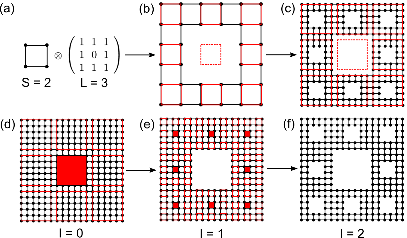
Figure 7: Schematic plot of constructing Sierpiński carpet with $S=2$, $L=3$ and $I=2$ in (a)-(c) bottom-up and (d)-(f) top-down approaches. The dashed squares in (a)-(c) and filled squares in (d)-(f) indicate the void areas in the fractal.

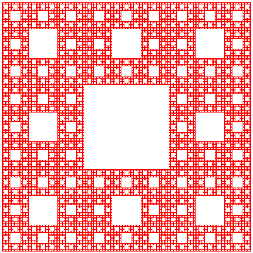
Figure 8: Sierpiński carpet with $S=2$, $L=3$ and $I=4$.

4.8 Strain and external fields

In this section, we introduce the common procedure of applying strain and external fields on the model. It is difficult to design common out-of-the-box user APIs that offer such functionalities since they are strongly case-dependent. Generally, the user should implement these perturbations by modifying model attributes such as orbital positions, on-site energies and hopping integrals. For the primitive cell, it is straightforward to achieve this goal with the set_orbital and add_hopping functions, as mentioned in section 3.2. The Sample class, on the contrary, does not offer such functions. Instead, the user should work with the attributes directly. In the Sample class, orbital positions and on-site energies are stored in the orb_pos and orb_eng attributes. Hopping terms are represented with 3 attributes: hop_i and hop_j for orbital indices, and hop_v for hopping integrals. There is also an auxiliary attribute dr which holds the hopping vectors. All the attributes are NumPy arrays. The on-site energies and hopping terms can be modified directly, while the orbital positions should be changed via a modifier function. The hopping vectors are updated from the orbital positions and hopping terms automatically, thus no need of explicit modification.

As the example, we will investigate the propagation of wave function in a graphene sample. We begin with defining the functions for adding strain and external fields, then calculate and plot the time-dependent wave function to check their effects on the propagation. The impact of magnetic field on electronic structure will also be discussed.

4.8.1 Functions for strain

Strain will introduce deformation into the model, changing both orbital positions and hopping integrals. It is a rule that orbital positions should not be modified directly, but through a modifier function. We consider a Gaussian bump deformation, and define the following function to generate the modifier

⬇

1def make_deform(center, sigma=0.5, extent=(1.0, 1.0), scale=(0.5, 0.5)):

2 def _deform(orb_pos):

3 x, y, z = orb_pos[:, 0], orb_pos[:, 1], orb_pos[:, 2]

4 dx = (x - center[0]) * extent[0]

5 dy = (y - center[1]) * extent[1]

6 amp = np.exp(-(dx**2 + dy**2) / (2 * sigma**2))

7 x += amp * dx * scale[0]

8 y += amp * dy * scale[0]

9 z += amp * scale[1]

10 return _deform

Here center, sigma and extent control the location, width and extent of the bump. For example, if extent is set to $(1.0,0.0)$, the bump will become one-dimensional which varies along $x$-direction while remains constant along $y$-direction. scale specifies the scaling factors for in-plane and out-of-plane displacements. The make_deform function returns another function as the modifier, which updates the orbital positions in place according to the following expression

$$\mathbf{r}_{i} \rightarrow\mathbf{r}_{i}+\Delta_{i},$$ (100)

$$\Delta_{i}^{\parallel} =A_{i}\cdot(\mathbf{r}_{i}^{\parallel}-\mathbf{c}_{0}^{\parallel})\cdot s^{\parallel},$$ (101)

$$\Delta_{i}^{\perp} =A_{i}\cdot s^{\perp},$$ (102)

$$A_{i} =\exp\left[-\frac{1}{2\sigma^{2}}\sum_{j=1}^{2}(\mathbf{r}_{i}^{j}-\mathbf{c}_{0}^{j})^{2}\cdot\eta^{j}\right],$$ (103)

where $\mathbf{r}_{i}$ is the position of $i$-th orbital, $\Delta_{i}$ is the displacement, $s$ is the scaling factor, $\parallel$ and $\perp$ are the in-plane and out-of-plane components. The location, width and extent of the bump are denoted as $\mathbf{c}_{0}$, $\sigma$ and $\eta$, respectively.

In addition to the orbital position modifier, we also need to update hopping integrals

⬇

1def update_hop(sample):

2 sample.init_hop()

3 sample.init_dr()

4 for i, rij in enumerate(sample.dr):

5 sample.hop_v[i] = calc_hop(rij)

As we will make use of the hopping terms and vectors, we should call the init_hop and init_dr functions to initialize the attributes. Similar rule holds for the on-site energies and orbital positions, as discussed in section 3.5. Then we loop over the hopping terms to update the integrals in hop_v according to the vectors in dr with the calc_hop function, which is defined in section 4.7.1.

4.8.2 Functions for external fields

The effects of external electric field can be modeled by adding position-dependent potential to the on-site energies. We consider a Gaussian-type scattering potential described by

$$V_{i}=V_{0}\cdot A_{i}$$ (104)

and define the following function to add the potential to the sample

⬇

1def add_efield(sample, center, sigma=0.5, extent=(1.0, 1.0), v_pot=1.0):

2 sample.init_orb_pos()

3 sample.init_orb_eng()

4 orb_pos = sample.orb_pos

5 orb_eng = sample.orb_eng

6 for i, pos in enumerate(orb_pos):

7 dx = (pos.item(0) - center[0]) * extent[0]

8 dy = (pos.item(1) - center[1]) * extent[1]

9 orb_eng[i] += v_pot * math.exp(-(dx**2 + dy**2) / (2 * sigma**2))

The arguments center, sigma and extent are similar to that of the make_deform function, while v_pot specifies $V_{0}$. Similar to update_hop, we need to call init_orb_pos and init_orb_eng to initialize orbital positions and on-site energies before accessing them. Then the position-dependent scattering potential is added to the on-site energies.

The effects of magnetic field can be modeled with Peierls substitution, as discussed in section 2. For homogeneous magnetic field perpendicular to the $xOy$-plane along $-z$ direction, the Sample class offers an API set_magnetic_field, which follows the Landau gauge of vector potential $\mathbf{A}=(By,0,0)$ and updates the hopping terms as

$$t_{ij}\rightarrow t_{ij}\cdot\exp\left[\mathrm{i}\frac{eB}{2\hbar c}\cdot(\mathbf{r}_{j}^{x}-\mathbf{r}_{i}^{x})\cdot(\mathbf{r}_{j}^{y}+\mathbf{r}_{i}^{y})\right]$$ (105)

where $B$ is the intensity of magnetic field, $\mathbf{r}_{i}$ and $\mathbf{r}_{j}$ are the positions of $i$-th and $j$-th orbitals, respectively.

4.8.3 Initial wave functions

The initial wave function we consider here as an example for the propagation is a Gaussian wave-packet, which is defined by

⬇

1def init_wfc_gaussian(sample, center, sigma=0.5, extent=(1.0, 1.0)):

2 sample.init_orb_pos()

3 orb_pos = sample.orb_pos

4 wfc = np.zeros(orb_pos.shape[0], dtype=np.complex128)

5 for i, pos in enumerate(orb_pos):

6 dx = (pos.item(0) - center[0]) * extent[0]

7 dy = (pos.item(1) - center[1]) * extent[1]

8 wfc[i] = math.exp(-(dx**2 + dy**2) / (2 * sigma**2))

9 wfc /= np.linalg.norm(wfc)

10 return wfc

Note that the wave function should be a complex vector whose length must be equal to the number of orbitals. Also, it should be normalized before being returned.

4.8.4 Propagation of wave function

We consider a rectangular graphene sample with $50\times 20\times 1$ primitive cells, as shown in Fig. 9(a). We begin with importing the necessary packages and defining some geometric parameters

⬇

1import math

2import numpy as np

3from numpy.linalg import norm

4import tbplas as tb

5

6prim_cell = tb.make_graphene_rect()

7dim = (50, 20, 1)

8pbc = (True, True, False)

9x_max = prim_cell.lat_vec[0, 0] * dim[0]

10y_max = prim_cell.lat_vec[1, 1] * dim[1]

11wfc_center = (x_max * 0.5, y_max * 0.5)

12deform_center = (x_max * 0.75, y_max * 0.5)

Here dim and pbc define the dimension and boundary condition. x_max and y_max are the lengths of the sample along $x$ and $y$ directions. The initial wave function will be a Gaussian wave-packet located at the center of the sample given by wfc_center. The deformation and scattering potential will be located at the center of right half of the sample, as specified by deform_center and shown in Fig. 9 (b)-(c).

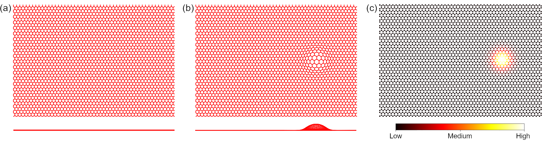
Figure 9: Top and side views of (a) pristine graphene sample and (b) sample with deformation. (c) Plot of on-site energies of graphene sample with scattering potential.

We firstly investigate the propagation of a one-dimensional Gaussian wave-packet in pristine sample, which is given by

⬇

1# Prepare the sample and inital wave function

2sample = tb.Sample(tb.SuperCell(prim_cell, dim, pbc))

3psi0 = init_wfc_gaussian(sample, center=wfc_center, extent=(1.0, 0.0))

4

5# Propagate the wave function

6config = tb.Config()

7config.generic["nr_time_steps"] = 128

8time_log = np.array([0, 16, 32, 64, 128])

9sample.rescale_ham()

10solver = tb.Solver(sample, config)

11psi_t = solver.calc_psi_t(psi0, time_log)

12

13# Visualize the time-dependent wave function

14vis = tb.Visualizer()

15for i in range(len(time_log)):

16 vis.plot_wfc(sample, np.abs(psi_t[i])**2, cmap="hot", scatter=False)

As the propagation is performed with the calc_psi_t function of Solver class, it follows the common procedure of TBPM calculation. We propagate the wave function by 128 steps, and save the snapshots in psi_t at the time steps specified in time_log. The snapshots are then visualized by the plot_wfc function of Visualizer class, as shown in Fig. 10(a)-(e), where the wave-packet diffuses freely, hits the boundary and forms interference pattern.

We then add the bump deformation to the sample, by assigning the modifier function to the supercell and calling update_hop to update the hopping terms

⬇

1deform = make_deform(center=deform_center)

2sample = tb.Sample(tb.SuperCell(prim_cell, dim, pbc, orb_pos_modifier=deform))

3update_hop(sample)

The propagation of wave-packet in deformed graphene sample is shown in Fig. 10(f)-(j). Obviously, the wave function gets scattered by the bump. Although similar interference pattern is formed, the propagation in the right part of the sample is significantly hindered, due to the increased inter-atomic distances and reduced hopping integrals at the bump.

Similar phenomena are observed when the scattering potential is added to the sample by

⬇

1add_efield(sample, center=deform_center)

The time-dependent wave function is shown in Fig. 10(k)-(o). Due to the higher on-site energies, the probability of emergence of electron is suppressed near the scattering center.

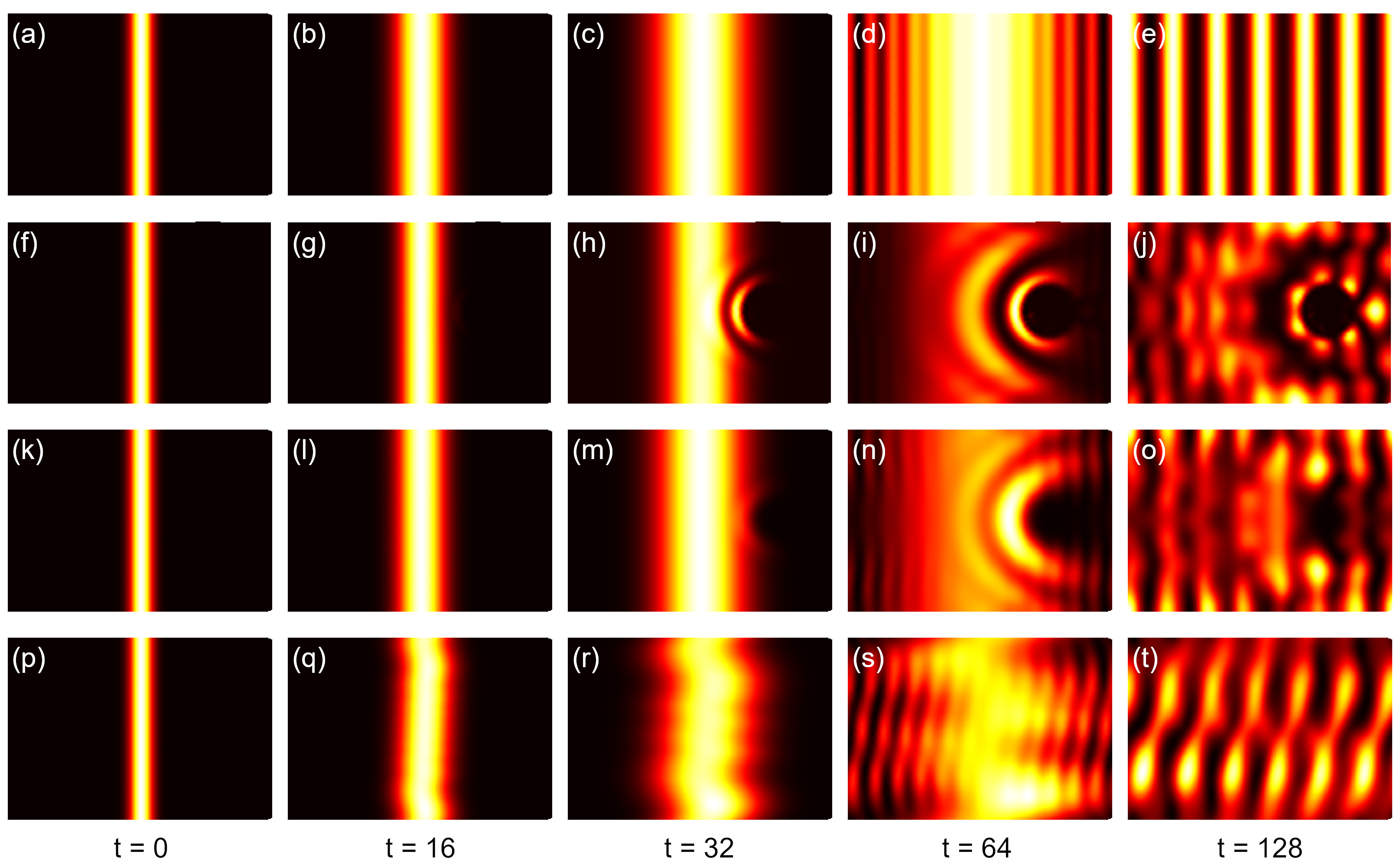
Figure 10: (a)-(e) Propagation of one-dimensional Gaussian wave-packet in pristine graphene sample. (f)-(j) Propagation in graphene sample with deformation, (k)-(o) with scattering potential and (p)-(t) with magnetic field of 50 Tesla.

As for the effects of magnetic field, it is well known that Landau levels will emerge in the DOS, as shown in Fig. 4(d). The analytical solution to Schrödinger’s equation for free electron in homogeneous magnetic field with $\mathbf{A}=(By,0,0)$ shows that the wave function will propagate freely along $x$ and $z$-directions while oscillates along $y$-direction. To simulate this process, we apply the magnetic field to the sample by

⬇

1sample.set_magnetic_field(50)

The snapshots of time-dependent wave function are shown in Fig. 10(p)-(t). The interference pattern is similar to the case without magnetic field, as the wave function propagates freely along $x$ direction. However, due to the oscillation along $y$-direction, the interference pattern gets distorted during the propagation. These phenomena agree well with the analytical results.

4.9 Miscellaneous

4.9.1 Wannier90 interface, Slater-Koster formula and parameter fitting

In this section, we demonstrate the usage of Wannier90 interface wan2pc, Slater-Koster table SK and parameter fitting tool ParamFit, by reducing an 8-band graphene primitive cell imported from the output of Wannier90. We achieve this by truncating the hopping terms to the second nearest neighbor, and refitting the on-site energies and Slater-Koster parameters to minimize the residual between the reference and fitted band data, i.e.,

$$\min_{\mathbf{x}}\sum_{i,\mathbf{k}}\omega_{i}\left|\bar{E}_{i,\mathbf{k}}-E_{i,\mathbf{k}}(\mathbf{x})\right|^{2}$$ (106)

where $\mathbf{x}$ are the fitting parameters, $\omega$ are the fitting weights, $\bar{E}$ and $E$ are the reference and fitted band data from the original and reduced cells, $i$ and $\mathbf{k}$ are band and $\mathbf{k}$-point indices, respectively.

We begin with importing the necessary packages

⬇

1import numpy as np

2import matplotlib.pyplot as plt

3import tbplas as tb

and define the following function to build the primitive cell from the Slater-Koster parameters

⬇

1def make_cell(sk_params):

2 # Lattice constants and orbital info.

3 lat_vec = np.array([

4 [2.458075766398899, 0.000000000000000, 0.000000000000000],

5 [-1.229037883199450, 2.128755065595607, 0.000000000000000],

6 [0.000000000000000, 0.000000000000000, 15.000014072326660],

7 ])

8 orb_pos = np.array([

9 [0.000000000, 0.000000000, 0.000000000],

10 [0.666666667, 0.333333333, 0.000000000],

11 ])

12 orb_label = ("s", "px", "py", "pz")

13

14 # Create the cell and add orbitals

15 e_s, e_p = sk_params[0], sk_params[1]

16 cell = tb.PrimitiveCell(lat_vec, unit=tb.ANG)

17 for pos in orb_pos:

18 for label in orb_label:

19 if label == "s":

20 cell.add_orbital(pos, energy=e_s, label=label)

21 else:

22 cell.add_orbital(pos, energy=e_p, label=label)

23

24 # Add Hopping terms

25 neighbors = tb.find_neighbors(cell, a_max=5, b_max=5,

26 max_distance=0.25)

27 sk = tb.SK()

28 for term in neighbors:

29 i, j = term.pair

30 label_i = cell.get_orbital(i).label

31 label_j = cell.get_orbital(j).label

32 hop = calc_hop(sk, term.rij, term.distance, label_i, label_j,

33 sk_params)

34 cell.add_hopping(term.rn, i, j, hop)

35 return cell

In line 3-12 we define the lattice vectors, orbital positions and labels. The SK class will utilize the orbital labels to evaluate the hopping integrals, so they must be chosen from a set of predefined strings, namely s for $s$ orbitals, px/py/pz for $p$ orbitals, and dxy/dx2-y2/dyz/dzx/dz2 for $d$ orbitals, respectively. Then in line 15-22 we add the orbitals with on-site energies taken from the first 2 elements of sk_params and the predefined labels. In line 25 we call find_neighbors to find all the orbital pairs within the cutoff distance of 0.25 nm, where the arguments a_max and b_max specify the searching range. After that, we create a Slater-Koster table from the SK class, and loop over the orbital pairs to add the hopping terms, which are evaluated by the calc_hop function depending on the displacement vector rij, the distance distance, orbital labels label_i and label_j, and Slater-Koster parameters sk_params. The calc_hop function is defined as

⬇

1def calc_hop(sk, rij, distance, label_i, label_j, sk_params):

2 # 1st and 2nd hopping distances in nm

3 d1 = 0.1419170044439990

4 d2 = 0.2458074906840380

5 if abs(distance - d1) < 1.0e-5:

6 v_sss, v_sps, v_pps, v_ppp = sk_params[2:6]

7 elif abs(distance - d2) < 1.0e-5:

8 v_sss, v_sps, v_pps, v_ppp = sk_params[6:10]

9 else:

10 raise ValueError(f"Too large distance {distance}")

11 return sk.eval(r=rij, label_i=label_i, label_j=label_j,

12 v_sss=v_sss, v_sps=v_sps,

13 v_pps=v_pps, v_ppp=v_ppp)

where we extract the first and second-nearest Slater-Koster parameters from sk_params, and call the eval function of SK class to evaluate the hopping integral, taking the displacement vector, orbital labels and SK parameters as input.

The fitting tool ParamFit is an abstract class. The users should derive their own fitting class from it, and implement the calc_bands_ref and calc_bands_fit functions, which return the reference and fitted band data, respectively. We define a MyFit class as

⬇

1class MyFit(tb.ParamFit):

2 def calc_bands_ref(self):

3 cell = tb.wan2pc("graphene")

4 k_len, bands = cell.calc_bands(self.k_points)

5 return bands

6

7 def calc_bands_fit(self, sk_params):

8 cell = make_cell(sk_params)

9 k_len, bands = cell.calc_bands(self.k_points, echo_details=False)

10 return bands

In calc_bands_ref, we import the primitive cell with the Wannier90 interface wan2pc, then calculate and return the band data. The calc_bands_fit function does a similar job, with the only difference that the primitive cell is constructed from Slater-Koster parameters with the make_cell function we have just created.

The application of MyFit class is as following

⬇

1def main():

2 # Fit the sk parameters

3 k_points = tb.gen_kmesh((120, 120, 1))

4 weights = np.array([0.1, 0.1, 1.0, 1.0, 1.0, 1.0, 0.1, 0.1])

5 fit = MyFit(k_points, weights)

6 sk0 = np.array([-8.370, 0.0,

7 -5.729, 5.618, 6.050, -3.070,

8 0.102, -0.171, -0.377, 0.070])

9 sk1 = fit.fit(sk0)

10 print("SK parameters after fitting:")

11 print(sk1[:2])

12 print(sk1[2:6])

13 print(sk1[6:10])

14

15 # Plot fitted band structure

16 cell_ref = tb.wan2pc("graphene")

17 cell_fit = make_cell(sk1)

18 k_points = np.array([

19 [0.0, 0.0, 0.0],

20 [1./3, 1./3, 0.0],

21 [1./2, 0.0, 0.0],

22 [0.0, 0.0, 0.0],

23 ])

24 k_path, k_idx = tb.gen_kpath(k_points, [40, 40, 40])

25 k_len, bands_ref = cell_ref.calc_bands(k_path)

26 k_len, bands_fit = cell_fit.calc_bands(k_path)

27 num_bands = bands_ref.shape[1]

28 for i in range(num_bands):

29 plt.plot(k_len, bands_ref[:, i], color="red", linewidth=1.0)

30 plt.plot(k_len, bands_fit[:, i], color="blue", linewidth=1.0)

31 plt.show()

32

33

34if __name__ == "__main__":

35 main()

To create a ParamFit instance, we need to specify the $\mathbf{k}$-points and fitting weights, as shown in line 3-4. For the $\mathbf{k}$-points, we are going to use a $\mathbf{k}$-grid of $120\times 120\times 1$. The length of weights should be equal to the number of orbitals of the primitive cell, which is 8 in our case. We assume all the bands to have the same weights, and set them to 1. Then we create the ParamFit instance, define the initial guess of parameters from Ref. [84], and get the fitted results with the fit function. The output should look like

⬇

1SK parameters after fitting:

2[-3.63102899 -1.08477167]

3[-5.27742318 5.87219052 4.61650991 -2.75652966]

4[-0.24734558 0.17599166 0.14798703 0.16545428]

The first two numbers are the on-site energies for $s$ and $p$ orbitals, while the following numbers are the Slater-Koster paramets $V_{ss\sigma}$, $V_{sp\sigma}$, $V_{pp\sigma}$ and $V_{pp\pi}$ at first and second nearest hopping distances, respectively. We can also plot and compare the band structures from the reference and fitted primitive cells, as shown in Fig. 11(a). It is clear that the fitted band structure agrees well with the reference data near the Fermi level (-1.7 eV) and at deep (-20 eV) or high energies (10 eV). However, the derivation from reference data of intermediate bands (-5 eV and 5 eV) is non-negligible. To improve this, we lower the weights of band 1-2 and 7-8 by

⬇

1weights = np.array([0.1, 0.1, 1.0, 1.0, 1.0, 1.0, 0.1, 0.1])

and refitting the parameters. The results are shown in Fig. 11(b), where the fitted and reference band structures agree well from -5 to 5 eV.

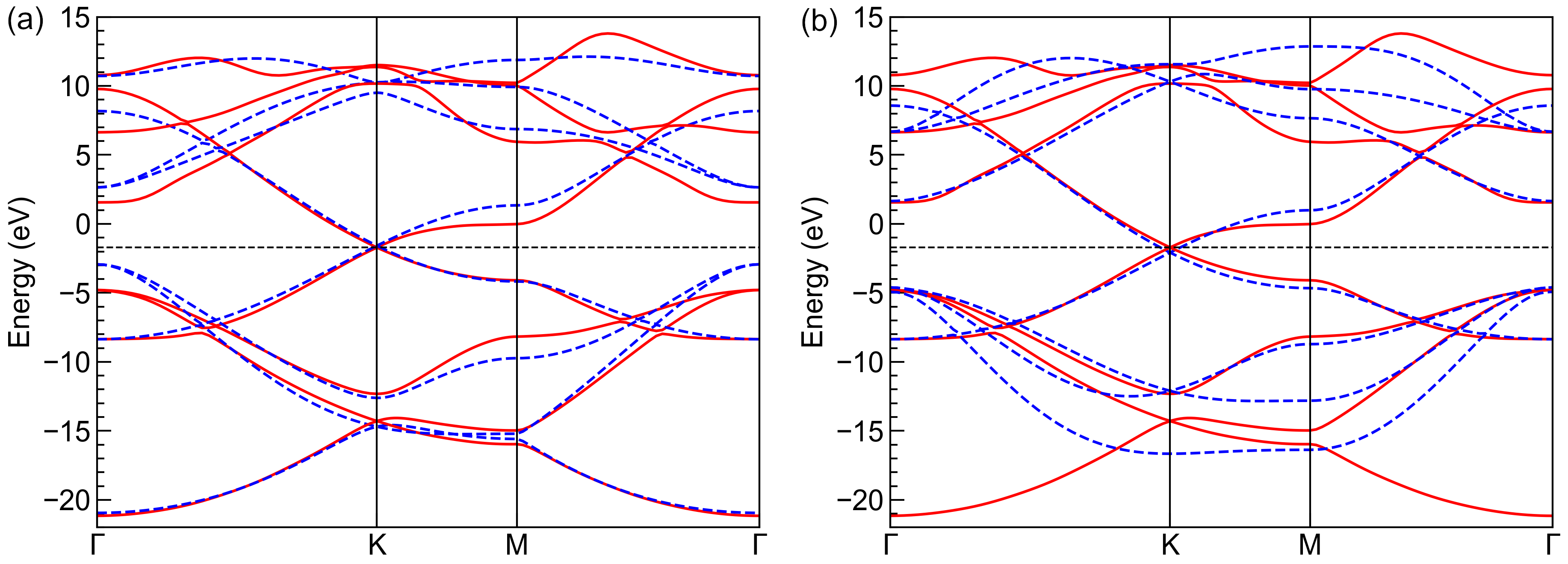
Figure 11: Band structures from reference (solid red lines) and fitted (dashed blue lines) primitive cells with (a) equal weights for all bands and (b) lower weights for bands 1-2 and 7-8. The horizontal dashed black lines indicate the Fermi level.

4.9.2 $\mathbb{Z}_{2}$ topological invariant and spin-orbital coupling

In this section, we demonstrate the usage of Z2 and SOC classes by calculating the topological invariant of bilayer bismuth [85] and check the effects of SOC. We consider the intra-atom SOC term

$$H^{\mathrm{soc}}=\lambda\mathbf{L}\cdot\mathbf{S}$$ (107)

and evaluate its matrix elements in the direct product basis of $|l\rangle\otimes|s\rangle$, where $|l\rangle$ are the $s$/$p$/$d$ orbitals and $|s\rangle$ are the eigenstates of Pauli matrix $\sigma_{z}$. We prefer this basis set because it does not require the evaluation of Clebsch-Gordan coefficients, thus much easier to implement. In this basis, the matrix element of SOC becomes

$$H_{ij}^{\mathrm{soc}}=\lambda\langle\mathbf{L}\cdot\mathbf{S}\rangle_{ij}=\lambda\langle l_{i},s_{i}\left|\mathbf{L}\cdot\mathbf{S}\right|l_{j},s_{j}\rangle$$ (108)

The eval function of SOC class calculates $\langle\mathbf{L}\cdot\mathbf{S}\rangle_{ij}$ taking the orbital and spin labels as input. The orbital labels should follow the notations in 4.9.1, while the spin labels should be either up or down. In actual calculations, we firstly double the orbitals and hopping terms in the primitive cell to yield the product basis, then add SOC as hopping terms between basis functions following Eq. (108).

We begin with importing the necessary packages

⬇

1from math import sqrt, pi

2import numpy as np

3from numpy.linalg import norm

4import tbplas as tb

5import tbplas.builder.exceptions as exc

Then we define the function to build the primitive cell without SOC

⬇

1def make_cell():

2 # Lattice constants

3 a = 4.5332

4 c = 11.7967

5 mu = 0.2341

6

7 # Lattice vectors of bulk

8 a1 = np.array([-0.5*a, -sqrt(3)/6*a, c/3])

9 a2 = np.array([0.5*a, -sqrt(3)/6*a, c/3])

10 a3 = np.array([0, sqrt(3)/3*a, c/3])

11

12 # Lattice vectors and atomic positions of bilayer

13 a1_2d = a2 - a1

14 a2_2d = a3 - a1

15 a3_2d = np.array([0, 0, c])

16 lat_vec = np.array([a1_2d, a2_2d, a3_2d])

17 atom_position = np.array([[0, 0, 0], [1/3, 1/3, 2*mu-1/3]])

18

19 # Create cell and add orbitals

20 cell = tb.PrimitiveCell(lat_vec, unit=tb.ANG)

21 atom_label = ("Bi1", "Bi2")

22 e_s, e_p = -10.906, -0.486

23 orbital_energy = {"s": e_s, "px": e_p, "py": e_p, "pz": e_p}

24 for i, pos in enumerate(atom_position):

25 for orbital, energy in orbital_energy.items():

26 label = f"{atom_label[i]}:{orbital}"

27 cell.add_orbital(pos, label=label, energy=energy)

28

29 # Add hopping terms

30 neighbors = tb.find_neighbors(cell, a_max=5, b_max=5, max_distance=0.454)

31 sk = tb.SK()

32 for term in neighbors:

33 i, j = term.pair

34 label_i = cell.get_orbital(i).label

35 label_j = cell.get_orbital(j).label

36 hop = calc_hop(sk, term.rij, label_i, label_j)

37 cell.add_hopping(term.rn, i, j, hop)

38 return cell

The make_cell function is much similar to that of section 4.9.1, where we firstly define the lattice vectors and orbital positions according to Ref. [85, 86], then add the orbitals and hopping terms using Slater-Koster formulation. Note that we have included atom labels in the orbital labels, namely Bi1 and Bi2, in order to distinguish the intra-atom terms when adding SOC afterwards. The hopping terms are evaluated by the calc_hop function, which is also similar to that of section 4.9.1

⬇

1def calc_hop(sk, rij, label_i, label_j):

2 dict1 = {"v_sss": -0.608, "v_sps": 1.320, "v_pps": 1.854, "v_ppp": -0.600}

3 dict2 = {"v_sss": -0.384, "v_sps": 0.433, "v_pps": 1.396, "v_ppp": -0.344}

4 dict3 = {"v_sss": 0.0, "v_sps": 0.0, "v_pps": 0.156, "v_ppp": 0.0}

5 r_norm = norm(rij)

6 if abs(r_norm - 0.30628728) < 1.0e-5:

7 data = dict1

8 elif abs(r_norm - 0.35116131) < 1.0e-5:

9 data = dict2

10 else:

11 data = dict3

12 lm_i = label_i.split(":")[1]

13 lm_j = label_j.split(":")[1]

14 return sk.eval(r=rij, label_i=lm_i, label_j=lm_j,

15 v_sss=data["v_sss"], v_sps=data["v_sps"],

16 v_pps=data["v_pps"], v_ppp=data["v_ppp"])

The intra-atom SOC is implemented in the add_soc function, which is defined as

⬇

1def add_soc(cell):

2 # Double the orbitals and hopping terms

3 cell = tb.merge_prim_cell(cell, cell)

4

5 # Add spin notations to the orbitals

6 num_orb_half = cell.num_orb // 2

7 num_orb_total = cell.num_orb

8 for i in range(num_orb_half):

9 label = cell.get_orbital(i).label

10 cell.set_orbital(i, label=f"{label}:up")

11 for i in range(num_orb_half, num_orb_total):

12 label = cell.get_orbital(i).label

13 cell.set_orbital(i, label=f"{label}:down")

14

15 # Add SOC terms

16 soc_lambda = 1.5

17 soc = tb.SOC()

18 for i in range(num_orb_total):

19 label_i = cell.get_orbital(i).label.split(":")

20 atom_i, lm_i, spin_i = label_i

21

22 for j in range(i+1, num_orb_total):

23 label_j = cell.get_orbital(j).label.split(":")

24 atom_j, lm_j, spin_j = label_j

25

26 if atom_j == atom_i:

27 soc_intensity = soc.eval(label_i=lm_i, spin_i=spin_i,

28 label_j=lm_j, spin_j=spin_j)

29 soc_intensity *= soc_lambda

30 if abs(soc_intensity) >= 1.0e-15:

31 try:

32 energy = cell.get_hopping((0, 0, 0), i, j)

33 except exc.PCHopNotFoundError:

34 energy = 0.0

35 energy += soc_intensity

36 cell.add_hopping((0, 0, 0), i, j, soc_intensity)

37 return cell

In line 3-13, we double the orbitals and hopping terms and add spin labels to the orbitals. Then we define the spin-orbital coupling intensity $\lambda$ and create an SOC instance in 16-17. Afterwards, we loop over the upper-triangular orbital pairs to add the SOC terms, while the conjugate terms are handled automatically. In line 26 we check if the two orbitals reside on the same atom, while in line 27 we call the eval function to calcualte the matrix element $\langle\mathbf{L}\cdot\mathbf{S}\rangle_{ij}$. If the corresponding hopping term already exists, the SOC term will be added to it. Otherwise, a new hopping term will be created.

With all the auxiliary functions ready, we now proceed to calculate the $\mathbb{Z}_{2}$ invariant number of bilayer bismuth

⬇

1def main():

2 # Create cell and add soc

3 cell = make_cell()

4 cell = add_soc(cell)

5

6 # Evaluate Z2

7 ka_array = np.linspace(-0.5, 0.5, 200)

8 kb_array = np.linspace(0.0, 0.5, 200)

9 kc = 0.0

10 z2 = tb.Z2(cell, num_occ=10)

11 kb_array, phases = z2.calc_phases(ka_array, kb_array, kc)

12

13 # Plot phases

14 vis = tb.Visualizer()

15 vis.plot_phases(kb_array, phases / pi)

16

17

18if __name__ == "__main__":

19 main()

To calculate $\mathbb{Z}_{2}$ we need to sample the $\mathbf{k}_{a}$ from $-\frac{1}{2}\mathbf{G}_{a}$ to $\frac{1}{2}\mathbf{G}_{a}$, and $\mathbf{k}_{b}$ from $\mathbf{0}$ to $\frac{1}{2}\mathbf{G}_{b}$. Then we create a Z2 instance and its calc_phases function to get the topological phases $\theta_{m}^{D}$ defined in Eq. (92). After that, we plot $\theta_{m}^{D}$ as the function of $\mathbf{k}_{b}$ in Fig. 12(a). It is clear that the crossing number of phases against the reference line is 1, indicating that bilayer bismuth is a topological insulator. We then decrease the SOC intensity $\lambda$ to 0.15 eV and re-calculate the phases. The results are shown in Fig. 12(b), where the crossing number is 0, indicating that bilayer bismuth becomes a normal insulator under weak SOC, similar to the case of bilayer Sb [76].

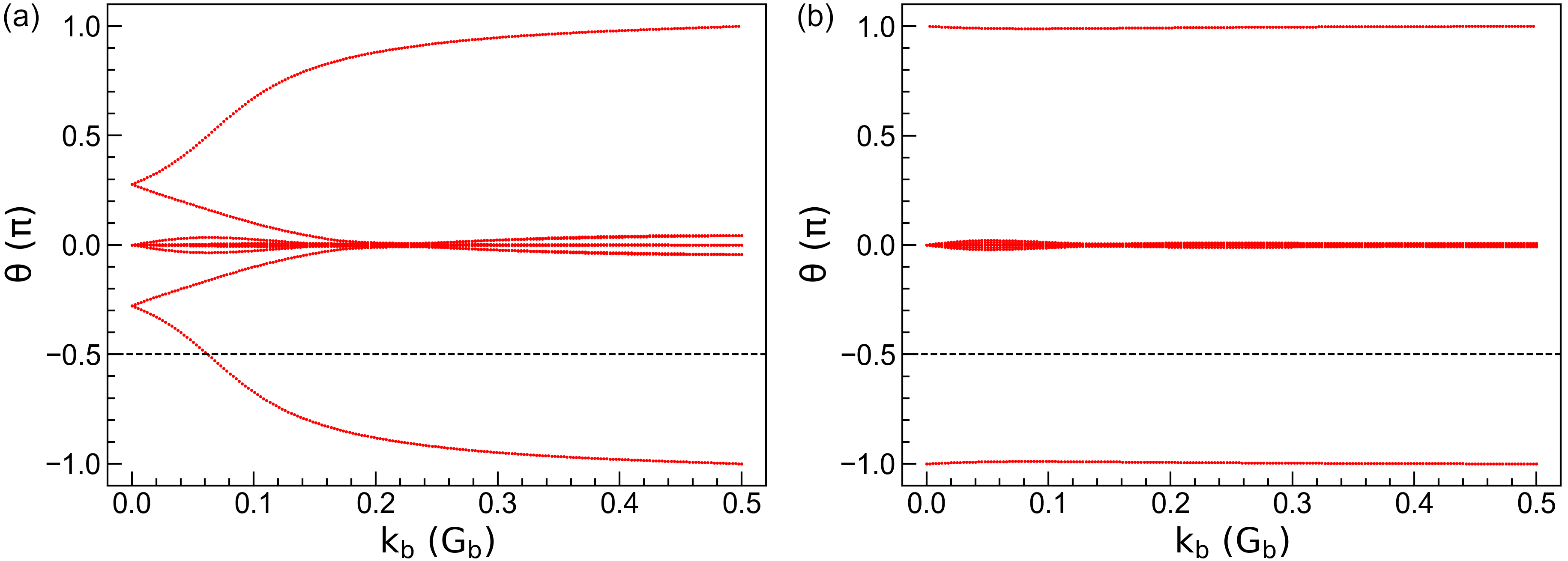
Figure 12: Topological phases $\theta_{m}^{D}$ of bilayer bismuth under SOC intensity of (a) $\lambda$ = 1.5 eV and (b) $\lambda$ = 0.15 eV. The horizontal dashed lines indicates the reference lines with which the crossing number is determined.

4.10 Parallelization

In this section, we give the general guidelines to set up the parallelization environment and show how to run calculations in parallel mode within TBPLaS. It should be noted that the determination of optimal parallelization configuration is a non-trivial task and strongly case-dependent. So, the guidelines provided here serve only as a starting point, whereas intensive tests and benchmarks are required before production runs.

4.10.1 General guidelines

The technical details of parallelism of TBPLaS have been discussed in section 3.7. Up to now, hybrid MPI+OpenMP parallelization has been implemented for the evaluation of band structure and DOS from exact-diagonalization, response properties from Lindhard function, topological invariant $\mathbb{Z}_{2}$ and TBPM calculations. Both MPI and OpenMP can be switched on/off separately on demand, while pure OpenMP mode is enabled by default.

The number of OpenMP threads is controlled by the OMP_NUM_THREADS environment variable. If TBPLaS has been compiled with MKL support, then the MKL_NUM_THREADS environment variable will also take effect. If none of the environment variables has been set, OpenMP will make use of all the CPU cores on the computing node. To switch off OpenMP, set the environment variables to 1. On the contrary, MPI-based parallelization is disabled by default, but can be easily enabled with a single option. The calc_bands and calc_dos functions of PrimitiveCell and Sample classes, the initialization functions of Lindhard, Z2, Solver and Analyzer classes all accept an argument named enable_mpi whose default value is taken to be False. If set to True, MPI-based parallelization is turned on, provided that the MPI4PY package has been installed. Hybrid MPI+OpenMP parallelization is achieved by enabling MPI and OpenMP simultaneously. The number of processes is controlled by the MPI launcher, which receives arguments from the command line, environment variables or configuration file. The user is recommended to check the manual of job queuing system on the computer for properly setting the environment variables and invoking the MPI launcher. For computers without a queuing system, e.g., laptops, desktops and standalone workstations, the MPI launcher should be mpirun or mpiexec, while the number of processes is controlled by the -np command line option.

The optimal parallelization configuration, i.e., the numbers of MPI processes and OpenMP threads, depend on the hardware, the model size and the type of calculation. Generally speaking, matrix diagonalization for a single $\mathbf{k}$-point is poorly parallelized over threads. But the diagonalization for multiple $\mathbf{k}$-points can be efficiently parallelized over processes. Therefore, for band structure and DOS calculations, as well as response properties from Lindhard function and topological invariant from Z2, it is recommended to run in pure MPI-mode by setting the number of MPI processes to the total number of allocated CPU cores and the number of OpenMP threads to 1. However, MPI-based parallelization uses more RAM since every process has to keep a copy of the wave functions and energies. So, if the available RAM imposes a limit, try to use less processes and more threads. Anyway, the product of the numbers of processes and threads should be equal to the number of allocated CPU cores. For example, if you have allocated 16 cores, then you can try 16 processes $\times$ 1 thread, 8 processes $\times$ 2 threads, 4 processes $\times$ 4 threads, etc. For TBPM calculations, the number of random initial wave functions should be divisible by the number of processes. For example, if you are going to consider 16 initial wave functions, then the number of processes should be 1, 2, 4, 8, or 16. The number of threads should be set according to the number of processes. Again, if the RAM size is a problem, try to decrease the number of processes and increase the number of threads.

If MPI-based parallelization is enabled, either in pure MPI or hybrid MPI+OpenMP mode, special care should be taken to output and plotting part of the job script. These operations should be performed on the master process only, otherwise the output will mess up or files get corrupted, since all the processes will try to modify the same file or plotting the same data. This situation is avoided by checking the rank of the process before action. The Lindhard, Z2, Solver, Analyzer and Visualizer classes all offer an is_master attribute to detect the master process, whose usage will be demonstrated in the following sections.

Last but not least, we have to mention that all the calculations in previous sections can be run in either interactive or batch mode. You can input the script line-by-line in the terminal, or save it to a file and pass the file to the Python interpreter. However, MPI-based parallelization supports only the batch mode, since there is no possibility to input anything in the terminal for multiple processes in one time. In the following sections, we assume the script file to be test_mpi.py. A common head block of the script is given in 4.10.2 and will not be explicitly repeated in subsequent sections.

4.10.2 Band structure and DOS

We demonstrate the usage of calc_bands and calc_dos in parallel mode by calculating the band structure and DOS of a $12\times 12\times 1$ graphene sample. Procedure shown here is also valid for the primitive cell. To enable MPI-based parallelization, we need to save the script to a file, for instance, test_mpi.py. The head block of this file should be

⬇

1#! /usr/bin/env python

2

3import numpy as np

4import tbplas as tb

5

6

7timer = tb.Timer()

8vis = tb.Visualizer(enable_mpi=True)

where the first line is a magic line declaring that the script should be interpreted by the Python program. In the following lines we import the necessary packages. To record and report the time usage, we need to create a timer from the Timer class. We also need a visualizer for plotting the results, where the enable_mpi argument is set to True during initialization. This head block also is essential for other examples in subsequent sections.

For convenience, we will not build the primitive cell from scratch, but import it from the material repository with the make_graphene_diamond function

⬇

1cell = tb.make_graphene_diamond()

Then we build the sample by

⬇

1sample = tb.Sample(tb.SuperCell(cell, dim=(12, 12, 1), pbc=(True, True, False)))

The evaluation of band structure in parallel mode is similar to the serial mode, which also involves generating the $\mathbf{k}$-path and calling calc_bands. The only difference is that we need to set the enable_mpi argument to True when calling calc_bands

⬇

1k_points = np.array([

2 [0.0, 0.0, 0.0],

3 [2./3, 1./3, 0.0],

4 [1./2, 0.0, 0.0],

5 [0.0, 0.0, 0.0],

6])

7k_path, k_idx = tb.gen_kpath(k_points, [40, 40, 40])

8timer.tic("band")

9k_len, bands = sample.calc_bands(k_path, enable_mpi=True)

10timer.toc("band")

11vis.plot_bands(k_len, bands, k_idx, k_label)

12if vis.is_master:

13 timer.report_total_time()

The tic and toc functions begin and end the recording of time usage, which receive a string as the argument for tagging the record. The visualizer is aware of the parallel environment, so no special treatment is needed when plotting the results. Finally, the time usage is reported with the report_total_time function on the master process only, by checking the is_master attribute of the visualizer.

We run test_mpi.py by

⬇

1$ export OMP_NUM_THREADS=1

2$ mpirun -np 1 ./test_mpi.py

With the environment variable OMP_NUM_THREADS set to 1, the script will run in pure MPI-mode. We invoke 1 MPI process by the -np option of the MPI launcher (mpirun). The output should look like

⬇

1 band : 11.03s

So, the evaluation of bands takes 11.03 seconds on 1 process. We try with more processes

⬇

1$ mpirun -np 2 ./test_mpi.py

2 band : 5.71s

3$ mpirun -np 4 ./test_mpi.py

4 band : 2.93s

Obviously, the time usage scales reversely with the number of processes. Detailed discussion on the time usage and speedup under different parallelization configurations will be discussed in section 4.10.6.

Evaluation of DOS can be parallelized in the same approach, by setting the enable_mpi argument to True

⬇

1k_mesh = tb.gen_kmesh((20, 20, 1))

2timer.tic("dos")

3energies, dos = sample.calc_dos(k_mesh, enable_mpi=True)

4timer.toc("dos")

5vis.plot_dos(energies, dos)

6if vis.is_master:

7 timer.report_total_time()

The script can be run in the same approach as evaluating the band structure.

4.10.3 Response properties from Lindhard function

To evaluate response properties in parallel mode, simply set the enable_mpi argument to True when creating the Lindhard calculator

⬇

1lind = tb.Lindhard(cell=cell, energy_max=10.0, energy_step=2048, kmesh_size=(600, 600, 1), mu=0.0, temperature=300.0, g_s=2, back_epsilon=1.0, dimension=2, enable_mpi=True)

Subsequent calls to the functions of Lindhard class does not need further special treatment. For example, the optical conductivity can be evaluated in the same approach as in serial mode

⬇

1timer.tic("ac_cond")

2omegas, ac_cond = lind.calc_ac_cond(component="xx")

3timer.toc("ac_cond")

4vis.plot_xy(omegas, ac_cond)

5if vis.is_master:

6 timer.report_total_time()

4.10.4 Topological invariant from Z2

The evaluation of phases $\theta_{m}^{D}$ can be paralleled in the same approach as response functions

⬇

1z2 = tb.Z2(cell, num_occ=10, enable_mpi=True)

2timer.tic("z2")

3kb_array, phases = z2.calc_phases(ka_array, kb_array, kc)

4timer.toc("z2")

5vis.plot_phases(kb_array, phases / pi)

6if vis.is_master:

7 timer.report_total_time()

where we only need to set enable_mpi argument to True when creating the Z2 instance.

4.10.5 Properties from TBPM

TBPM calculations in parallel mode are similar to the evaluation of response functions. The user only needs to set the enable_mpi argument to True. To make the time usage noticeable, we build a larger sample first

⬇

1sample = tb.Sample(tb.SuperCell(cell, dim=(240, 240, 1), pbc=(True, True, False)))

Then we create the configuration, solver and analyzer, with the argument enable_mpi=True

⬇

1sample.rescale_ham(9.0)

2config = tb.Config()

3config.generic["nr_random_samples"] = 4

4config.generic["nr_time_steps"] = 256

5solver = tb.Solver(sample, config, enable_mpi=True)

6analyzer = tb.Analyzer(sample, config, enable_mpi=True)

Correlation function can be obtained and analyzed in the same way as in serial mode

⬇

1timer.tic("corr_dos")

2corr_dos = solver.calc_corr_dos()

3timer.toc("corr_dos")

4energies, dos = analyzer.calc_dos(corr_dos)

5vis.plot_dos(energies, dos)

6if vis.is_master:

7 timer.report_total_time()

4.10.6 Benchmarks

The time usages and speedups of different types of calculations are summarized in Table 5. The benchmarks have been performed on an Intel^® Xeon^® Gold 6248 CPU, with 16 cores allocated at most. It is obvious that for the evaluation of band structure and DOS, increasing the number of MPI processes significantly boosts the calculation. However, the efficiency enhancement of increasing OpenMP threads is much lower. The average speedup drops significantly when OpenMP is enbaled, indicating a poor scaling versus the number of CPU cores. This is due to the fact that matrix diagonalization cannot be efficiently parallelized over threads. On the contrary, pure MPI-based parallelization has the best efficiency, with an almost linear scaling (average speedup $\approx 1$).

The evaluation of optical conductivity has an additional post-processing step after diagonalization, which is suitable for both MPI and OpenMP-based parallelization. So, the speedup and scaling versus the number of threads improve slightly. $\mathbb{Z}_{2}$ topological invariant shows a similar scaling behavior as band structure and DOS, i.e., pure MPI parallelization has the best efficiency. For TBPM calculations, the speedups and efficiencies of multi-threading and multi-processing are almost equal, since sparse matrix-vector multiplication can be efficiently parallelized over threads. Although pure MPI-mode still has the best efficiency, the number of processes is limited by the number of random initial wave functions and available RAM size, as discussed in section 4.10.1. So, pure OpenMP or hybrid MPI+OpenMP paralelization is recommended for TBPM calculations, with the optimal numbers of processes and and threads determined from benchmarks.

Table 5: Time usages and speedups of benchmarks for various calculation types with respect to the numbers of MPI processes ($n_{p}$) and OpenMP threads ($n_{t}$) per process. The standard ($t_{0}$) of each type is defined as the time usage on 1 process $\times$ 1 thread, while the speedup is defined as $t_{0}/t_{n_{p}n_{t}}$. Numbers in the brackets are the average speedups to each CPU core defined as $t_{0}/(t_{n_{p}n_{t}}\times n_{p}\times n_{t}$).

Type	$t_{0}/s$	$n_{p}$	$n_{t}$
			1	2	4
Band structure	2.56	1	1.00 (1.00)	1.19 (0.60)	1.45 (0.36)
		2	1.92 (0.96)	1.61 (0.40)	2.03 (0.25)
		4	4.00 (1.00)	3.05 (0.38)	4.06 (0.25)
DOS	10.62	1	1.00 (1.00)	1.17 (0.58)	1.33 (0.33)
		2	1.84 (0.92)	1.74 (0.44)	2.00 (0.25)
		4	3.74 (0.93)	3.23 (0.40)	3.88 (0.24)
Optical conductivity	24.45	1	1.00 (1.00)	1.58 (0.79)	2.25 (0.56)
		2	1.76 (0.88)	2.61 (0.65)	3.49 (0.44)
		4	3.30 (0.83)	4.57 (0.57)	5.93 (0.37)
$\mathbb{Z}_{2}$ invariant	34.37	1	1.00 (1.00)	0.99 (0.50)	1.00 (0.25)
		2	1.67 (0.84)	1.72 (0.43)	1.71 (0.21)
		4	3.32 (0.83)	3.34 (0.42)	3.38 (0.21)
TBPM	24.71	1	1.00 (1.00)	1.91 (0.96)	3.48 (0.87)
		2	1.96 (0.98)	3.80 (0.95)	6.84 (0.86)
		4	3.55 (0.89)	6.68 (0.83)	12.80 (0.80)

5 Examples

As mentioned in previous sections, TBPLaS is capable of tackling complex systems with tens of billions of atoms. In this section, we present an example utilizing TBPLaS to calculate the properties of TBG with magic angle $\theta=1.05^{\circ}$. For TBG with the magic angle, flat bands appear near the Fermi level, which provide a platform to explore strongly correlated phases and superconductivity [9, 12, 87]. The moiré supercell of twisted bilayer graphene is constructed by identifying a common periodicity between the two layers. We start with a AA stacking bilayer graphene ($\theta=0^{\circ}$), and choose the rotation origin (O) at an atom site. Then, we rotate one layer relatively to the other one by the angle $\theta$. Fig. 13 shows the atomic structure of the magic angle TBG. The moiré superlattice contains three types of high-symmetry staking patterns, namely AA, AB and BA stacking. For TBG with twist angles smaller that $1.2^{\circ}$, the system suffers significant lattice reconstruction due to the interplay between the interlayer van der Waals interaction and the in-plane strain field [88]. The lattice relaxation (both the out-of-plane and in-plane) of TBG is performed with the LAMMPS package [89]. The intralyer and interlayer interactions of TBG are simulated with the long-range carbon bond-order potential [90] and Kolmogorov-Crespi potential [91], respectively.

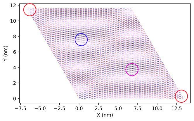
Figure 13: Atomic structure of TBG with twist angle $\theta=1.05^{\circ}$. Highly-symmetric stacking regions of AA, AB and BA are marked by red, blue and magenta circles, respectively. Carbon atoms in the top and bottom layers are depicted in blue and red, respectively.

The properties of both rigid (without lattice relaxation) and relaxed (with lattice relaxation) TBG with magic angle are calculated with a full tight-binding model based on $p_{z}$ orbitals [83]. The on-site energies $\epsilon_{i}$ are set to zero, and the hopping parameters between sites $i$ and $j$ are described by a distance-dependent function as

$$t_{ij}=n^{2}V_{pp\sigma}(r_{ij})+(1-n^{2})V_{pp\pi}(r_{ij})$$ (109)

where $r_{ij}=|\mathbf{r}_{ij}|$ is the distance between two sites located at $\mathbf{r}_{i}$ and $\mathbf{r}_{j}$, $n$ is the direction cosine of $\mathbf{r}_{ij}$ along the direction that is perpendicular to the graphene layer. The Slater-Koster parameters $V_{pp\sigma}$ and $V_{pp\pi}$ are

$$V_{pp\pi}(r_{ij}) =-t_{0}\mathrm{e}^{q_{\pi}(1-r_{ij}/d)}F_{c}(r_{ij})$$ (110)

$$V_{pp\sigma}(r_{ij}) =t_{1}\mathrm{e}^{q_{\sigma}(1-r_{ij}/h)}F_{c}(r_{ij})$$ (111)

where $d=1.42$ Å  and $h=3.349$ Å  are the nearest in-plane and out-of-plane carbon-carbon distances, respectively. $t_{0}=2.8$ eV and $t_{1}=0.44$ eV are re-optimized to obtain the magic angle at rotation angle $\theta=1.05^{\circ}$ [53]. The parameters $q_{\sigma}$ and $q_{\pi}$ satisfy $q_{\sigma}/h=q_{\pi}/d=2.218$ Å^-1, and the smooth function is defined as $F_{c}(r)=(1+\mathrm{e}^{(r-r_{c})/l_{c}})^{-1}$ with $l_{c}=0.265$ Åand $r_{c}=5.0$ Å.

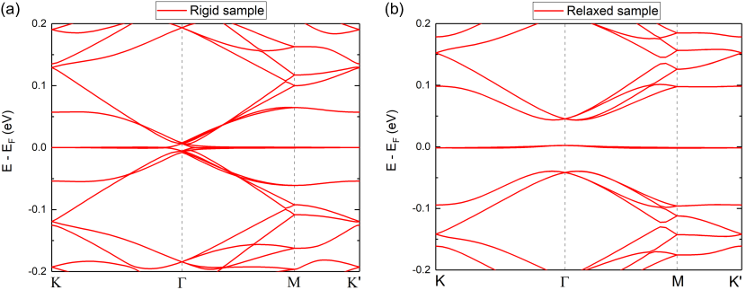
Figure 14: Band structures of (a) rigid and (b) relaxed TBG with $\theta=1.05^{\circ}$.

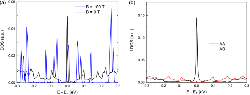
Figure 15: (a) Density of states of relaxed magic angle TBG with (blue line) and without (black line) magnetic field. (b) Local density of states of the highly-symmetric stacking regions of AA (black line) and AB (red line) in relaxed magic angle TBG.

Fig. 14 shows the band structure of rigid and relaxed TBG with twist angle $\theta=1.05^{\circ}$, which are obtained by exact diagonalization. In TBG without lattice relaxation (rigid sample), ultraflat bands appear in the charge neutrality. The bandwidth (energy difference between the K and $\Gamma$ points of the Brillouin zone) of the flat band is 7 meV, and the bandgap (energy difference between the flat band and the remote bands at the $\Gamma$ point) is zero. In relaxed sample (with lattice relaxation), the bandwidth and bandgap are 4 meV and 43 meV, respectively. Obviously, the lattice relaxation has a significant effect on the electronic structure of magic angle TBG. The black line in Fig. 15(a) is the density of states of relaxed TBG with magic angle, which is calculated via the TBPM in Eq. (42). In the calculations, the accuracy of the DOS can be guaranteed by utilizing a large enough model with more than ten million atoms. The number of time integration steps is 4096, which gives an energy resolution of 3.7 meV. In DOS a sharp peak appears in the charge neutrality, which corresponds to the flat bands. When a perpendicular magnetic field is applied, Landau levels appear in the DOS. The splitting of the peak around the energy $E=68$ meV is the lifting of the twofold degeneracy due to the Dirac point splitting in twisted bilayer graphene [92].

The LDOS is an important quantity to describe the local properties of a system, which can be utilized to simulate the $\mathrm{d}I/\mathrm{d}V$ spectra obtained with the STM in experiments. TBPLaS provides three approaches to evaluate the LDOS, i.e. exact-diagonalization, TBPM and the recursion method. Both TBPM and the recursion method are capable of dealing with very large models. The LDOS of different stacking regions in magic angle TBG obtained with TBPM are shown in Fig. 15. It is clear that the LDOS of the AA and AB regions have obvious different features. Only the LDOS of the AA region has a sharp peak at energy $E=0$, which means that the states of the flat bands are mainly localized in the AA region. The LDOS of the AB region has some peaks located at high energies. Such strong LDOS modulation shows spatially localized electronic states with specific energies, which can be justified by calculating the LDOS mapping (quasieigenstates) via Eq. (51). The LDOS mappings at different energies are shown in Fig. 16. At energy $E=0$, states are mainly localized in the AA regions. At the energy $E=-0.17$ eV, states are mainly localized in the AB and BA regions. Such periodic variation of the local electronic structure is a consequence of different interlayer couplings in TBG. The LDOS mapping is equivalent to the $\mathrm{d}I/\mathrm{d}V$ mapping observed experimentally with STM.

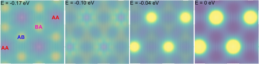
Figure 16: Local density of states mappings of magic angle TBG (with lattice relaxation) at energies $E=-0.17$ eV, $-0.10$ eV, $-0.04$ eV and $0$ eV.

In TBPLaS, we can also investigate the optical conductivity via the Kubo formula or the Lindhard function. The Lindhard function is more suitable for small models since it requires a diagonalization process. On the contrary, by combing the Kubo formula and TBPM, we can tackle large models that contain tens of millions of orbitals. In Fig. 17, the optical conductivity of the magic angle TBG and monolayer graphene is calculated with TBPM. Note that we omit the Drude weight part in the calculation. For TBG the peak with energy around $E=0.1$ eV is due to the transition between the flat bands and their adjacent bands. A dip-peak feature around $E=0.1$ eV is due to the electron-hole asymmetry [93].

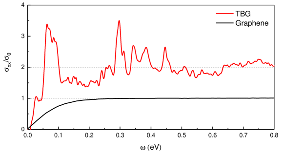
Figure 17: Optical conductivity of relaxed TBG with twist angle $\theta=1.05^{\circ}$ and monolayer graphene. The temperature is $T=300$ K and the chemical potential is $\mu=0$ eV.

In addition to the optical conductivity, many other response properties can also be obtained with TBPLaS. Fig. 18 shows the electron energy loss function of the magic angle TBG. Firstly, we calculate the dynamical polarization by using the Kubo formula in Eq. (76). Then the dielectric function and energy loss function are obtained within the random phase approximation with Eqs. (82) and (83), respectively. The plasmon mode can be detected by many experimental techniques, e.g. the scattering-type scanning near-field optical microscope (s-SNOM) and electron energy loss spectroscopy. In experiments, when a plasmon mode with frequency $\omega_{p}$ exists with low damping, the energy loss spectra possess a sharp peak at $\omega=\omega_{p}$. For the magic angle TBG, interband plasmon modes close to 100 meV appear at both temperature $T=300$ K and 1 K, which are attributed to the interband transitions from the flat bands to bands located at energy of 100 meV. These modes originate from the collective oscillations of electrons in the AA region [94]. The $\omega_{p}=100$ meV plasmon mode disperses within the particle-hole continuum in Figs. 18(c) and 18(d) with fast damping into electron-hole pairs. It becomes clear with a fine and flat shape with momentum larger than $0.2\;\mathrm{nm^{-1}}$. Single-particle transitions are almost forbidden in flat bands below 40 meV, corresponding to the value of band gap between the flat bands and the excited bands at $\Gamma$ point, from which the continuum spectrum rises to non-zero zone in Fig. 18 (c). When the temperature declines to the critical temperature 1 K at which the superconductivity can be detected in the magic-angle system [9], a thin plasmon mode with energy 9 meV emerges and stretches to large q in Fig. 18(b), which is contributed to the collective excitations among flat bands, i.e. flat-band plasmon. Meanwhile, underneath the collective flat-band plasmon mode, the particle-hole transitions arise with occupying a tiny energy region ranging from 0 meV to 8 meV in Fig. 18(d). As a result, this plasmon mode extends above the edge of this tiny energy zone and is free from the Laudau damping.

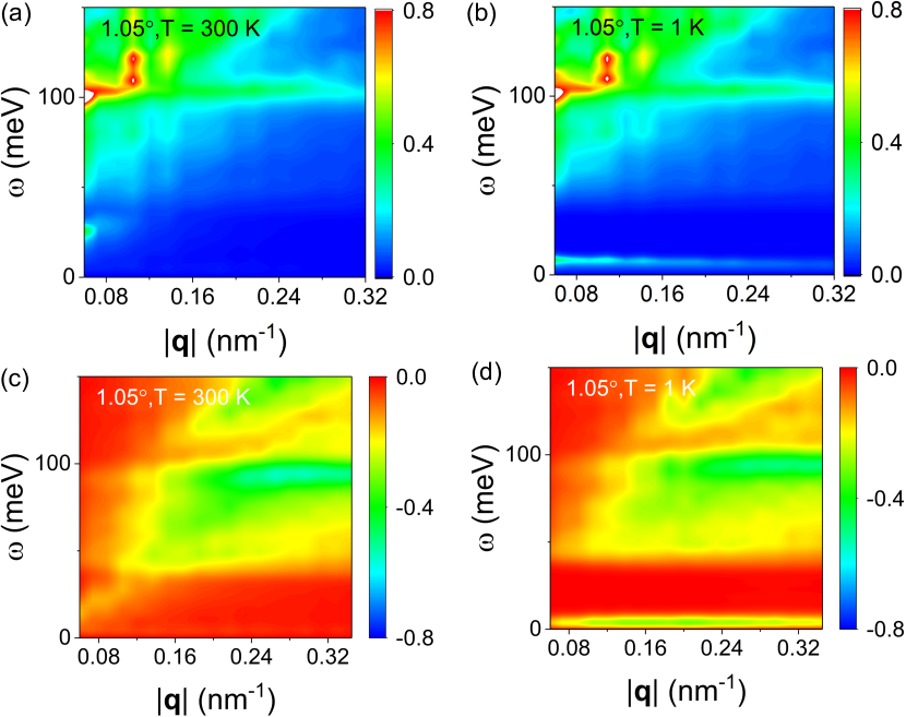
Figure 18: Plot of the loss function $-\mathrm{Im}\ \left[1/\epsilon(\mathbf{q},\omega)\right]$ as function of frequency $\omega$ and wave vector $\mathbf{q}$ for relaxed TBG with twist angel $\theta=1.05^{\circ}$ at temperatures (a) $T=300$ K and (b) $T=1$ K [53]. Plot of the particle-hole continuum $-\mathrm{Im}\ \Pi(\mathbf{q},\omega)$ with respect to the frequency $\omega$ and wave vector $\mathbf{q}$ at (c) $T=300$ K and (d) $T=1$ K. The chemical potential is $\mu=0$ and the background dielectric constant $\kappa=3.03$ of hBN substrate.

6 Summary

In summary, we have introduced the TBPLaS package, an open-source software suite for accurate electronic structure, optical properties, plasmon and transport calculations in real-space based on the tight-binding theory. It has an intuitive Python API for convenient simulation set-up, and Cython/Fortran cores for efficient performance. The main advantage of TBPLaS is that the numerical calculations is based on the TBPM without diagonalization. Both the memory and CPU costs have a linear scaling with the system size. So we can tackle models contain tens of millions of atoms or even billions of atoms if necessary. In addition to TBPM, exact diagonalization-based methods are also implemented. Moreover, crystalline defects, vacancies, adsorbates, charge impurity centres, strains and external perturbations can be easily and intuitively set up in TPLaS, which allows us to simulate large and complex models. With a wide range of pre-defined functions, the numerical calculations can be performed only with a few lines of code.

In the first release, TBPLaS already features a large variety of functionalities, e.g. the band structure, DOS, LDOS, wave functions, plasmon, optical conductivity, electric conductivity, Hall conductivity, quasi-eigenstate, real-space electron density and wave packet propagation. Moreover, thanks to its extensible and modular nature, it is easy to implemented other algorithms involving the tight-binding Hamiltonian. Further developments and extensions of TBPLaS, for instance, the real-space self-consistent Hartree and Hubbard methods for large systems [95, 96] and support for GPU acceleration, will be implemented in the future.

Acknowledgments  

We thank Edo van Veen, Guus Slotman, Kaixiang Huang, and Yalei Zhang for their contributions to the earlier version of the code. This work is supported by the National Natural Science Foundation of China (Grant No.12174291) and the National Key R&D Program of China (Grant No. 2018YFA0305800). Numerical calculations presented in this paper have been performed in the Supercomputing Center of Wuhan University.

Declaration of competing interest  

The authors declares no competing interests.

References

- [1] J. C. Slater and G. F. Koster. Simplified lcao method for the periodic potential problem. Phys. Rev., 94:1498–1524, Jun 1954.
- [2] CM Goringe, DR Bowler, and E Hernandez. Tight-binding modelling of materials. Rep. Prog. Phys., 60(12):1447, 1997.
- [3] Shengjun Yuan, Hans De Raedt, and Mikhail I. Katsnelson. Modeling electronic structure and transport properties of graphene with resonant scattering centers. Phys. Rev. B, 82:115448, Sep 2010.
- [4] Anthony Hams and Hans De Raedt. Fast algorithm for finding the eigenvalue distribution of very large matrices. Phys. Rev. E, 62:4365–4377, Sep 2000.
- [5] Shengjun Yuan, Rafael Roldán, and Mikhail I. Katsnelson. Excitation spectrum and high-energy plasmons in single-layer and multilayer graphene. Phys. Rev. B, 84(13):035439, Jul 2011.
- [6] R Logemann, KJA Reijnders, T Tudorovskiy, MI Katsnelson, and Shengjun Yuan. Modeling klein tunneling and caustics of electron waves in graphene. Phys. Rev. B, 91(4):045420, 2015.
- [7] G. J. Slotman, M. M. van Wijk, Pei-Liang Zhao, A. Fasolino, M. I. Katsnelson, and Shengjun Yuan. Effect of structural relaxation on the electronic structure of graphene on hexagonal boron nitride. Phys. Rev. Lett., 115:186801, Oct 2015.
- [8] R Haydock, Volker Heine, and MJ Kelly. Electronic structure based on the local atomic environment for tight-binding bands. J. Phys. C: Solid State Phys, 5(20):2845, 1972.
- [9] Yuan Cao, Valla Fatemi, Shiang Fang, Kenji Watanabe, Takashi Taniguchi, Efthimios Kaxiras, and Pablo Jarillo-Herrero. Unconventional superconductivity in magic-angle graphene superlattices. Nature, 556(7699):43–50, 2018.
- [10] Jeong Min Park, Yuan Cao, Kenji Watanabe, Takashi Taniguchi, and Pablo Jarillo-Herrero. Tunable strongly coupled superconductivity in magic-angle twisted trilayer graphene. Nature, 590(7845):249–255, 2021.
- [11] Haoxin Zhou, Ludwig Holleis, Yu Saito, Liam Cohen, William Huynh, Caitlin L Patterson, Fangyuan Yang, Takashi Taniguchi, Kenji Watanabe, and Andrea F Young. Isospin magnetism and spin-polarized superconductivity in bernal bilayer graphene. Science, 375(6582):774–778, 2022.
- [12] Yuan Cao, Valla Fatemi, Ahmet Demir, Shiang Fang, Spencer L Tomarken, Jason Y Luo, Javier D Sanchez-Yamagishi, Kenji Watanabe, Takashi Taniguchi, Efthimios Kaxiras, et al. Correlated insulator behaviour at half-filling in magic-angle graphene superlattices. Nature, 556(7699):80–84, 2018.
- [13] Yonglong Xie, Biao Lian, Berthold Jäck, Xiaomeng Liu, Cheng-Li Chiu, Kenji Watanabe, Takashi Taniguchi, B Andrei Bernevig, and Ali Yazdani. Spectroscopic signatures of many-body correlations in magic-angle twisted bilayer graphene. Nature, 572(7767):101–105, 2019.
- [14] Xiaobo Lu, Petr Stepanov, Wei Yang, Ming Xie, Mohammed Ali Aamir, Ipsita Das, Carles Urgell, Kenji Watanabe, Takashi Taniguchi, Guangyu Zhang, et al. Superconductors, orbital magnets and correlated states in magic-angle bilayer graphene. Nature, 574(7780):653–657, 2019.
- [15] Yuhang Jiang, Xinyuan Lai, Kenji Watanabe, Takashi Taniguchi, Kristjan Haule, Jinhai Mao, and Eva Y Andrei. Charge order and broken rotational symmetry in magic-angle twisted bilayer graphene. Nature, 573(7772):91–95, 2019.
- [16] Aaron L Sharpe, Eli J Fox, Arthur W Barnard, Joe Finney, Kenji Watanabe, Takashi Taniguchi, MA Kastner, and David Goldhaber-Gordon. Emergent ferromagnetism near three-quarters filling in twisted bilayer graphene. Science, 365(6453):605–608, 2019.
- [17] M Serlin, CL Tschirhart, H Polshyn, Y Zhang, J Zhu, K Watanabe, T Taniguchi, L Balents, and AF Young. Intrinsic quantized anomalous hall effect in a moiré heterostructure. Science, 367(6480):900–903, 2020.
- [18] Zhiren Zheng, Qiong Ma, Zhen Bi, Sergio de La Barrera, Ming-Hao Liu, Nannan Mao, Yang Zhang, Natasha Kiper, Kenji Watanabe, Takashi Taniguchi, et al. Unconventional ferroelectricity in moiré heterostructures. Nature, 588(7836):71–76, 2020.
- [19] Andre K Geim and Irina V Grigorieva. Van der waals heterostructures. Nature, 499(7459):419–425, 2013.
- [20] Stephen Carr, Shiang Fang, and Efthimios Kaxiras. Electronic-structure methods for twisted moiré layers. Nat Rev Mater, 5(10):748–763, 2020.
- [21] Bartholomew Andrews and Alexey Soluyanov. Fractional quantum hall states for moiré superstructures in the hofstadter regime. Phys. Rev. B, 101:235312, Jun 2020.
- [22] Jose H. García, Lucian Covaci, and Tatiana G. Rappoport. Real-space calculation of the conductivity tensor for disordered topological matter. Phys. Rev. Lett., 114:116602, Mar 2015.
- [23] Christoph W Groth, Michael Wimmer, Anton R Akhmerov, and Xavier Waintal. Kwant: a software package for quantum transport. New J. Phys., 16(6):063065, 2014.
- [24] Pythtb website. http://physics.rutgers.edu/pythtb/. Accessed: 25 July 2019.
- [25] Dean Moldovan, Miša Anđelković, and Francois Peeters. pybinding v0.9.5: a Python package for tight- binding calculations, August 2020. This work was supported by the Flemish Science Foundation (FWO-Vl) and the Methusalem Funding of the Flemish Government.
- [26] Alexander Weiße, Gerhard Wellein, Andreas Alvermann, and Holger Fehske. The kernel polynomial method. Rev. Mod. Phys., 78:275–306, Mar 2006.
- [27] Kristofer Björnson. Tbtk: A quantum mechanics software development kit. SoftwareX, 9:205–210, 2019.
- [28] Simão M João, Miša Anđelković, Lucian Covaci, Tatiana G Rappoport, João MVP Lopes, and Aires Ferreira. Kite: high-performance accurate modelling of electronic structure and response functions of large molecules, disordered crystals and heterostructures. R. Soc. open sci., 7(2):191809, 2020.
- [29] Aires Ferreira and Eduardo R Mucciolo. Critical delocalization of chiral zero energy modes in graphene. Phys. Rev. Lett., 115(10):106601, 2015.
- [30] Peter H Jacobse. Mathematb: A mathematica package for tight-binding calculations. Comput. Phys. Commun., 244:392–408, 2019.
- [31] Xueheng Kuang, Zhen Zhan, and Shengjun Yuan. Flat-band plasmons in twisted bilayer transition metal dichalcogenides. Phys. Rev. B, 105:245415, Jun 2022.
- [32] Haohao Shi, Zhen Zhan, Zhikai Qi, Kaixiang Huang, Edo van Veen, Jose Ángel Silva-Guillén, Runxiao Zhang, Pengju Li, Kun Xie, Hengxing Ji, et al. Large-area, periodic, and tunable intrinsic pseudo-magnetic fields in low-angle twisted bilayer graphene. Nat. Commun., 11(371):371, 2020.
- [33] Yi-Wen Liu, Zhen Zhan, Zewen Wu, Chao Yan, Shengjun Yuan, and Lin He. Realizing one-dimensional electronic states in graphene via coupled zeroth pseudo-landau levels. Phys. Rev. Lett., 129:056803, Jul 2022.
- [34] Shengjun Yuan, AN Rudenko, and MI Katsnelson. Transport and optical properties of single-and bilayer black phosphorus with defects. Phys. Rev. B, 91(11):115436, 2015.
- [35] Shengjun Yuan, Edo van Veen, Mikhail I Katsnelson, and Rafael Roldán. Quantum hall effect and semiconductor-to-semimetal transition in biased black phosphorus. Phys. Rev. B, 93(24):245433, 2016.
- [36] Shengjun Yuan, Malte Rösner, Alexander Schulz, Tim O Wehling, and Mikhail I Katsnelson. Electronic structures and optical properties of partially and fully fluorinated graphene. Phys. Rev. Lett., 114(4):047403, 2015.
- [37] Shengjun Yuan, Hans De Raedt, and Mikhail I Katsnelson. Electronic transport in disordered bilayer and trilayer graphene. Phys. Rev. B, 82(23):235409, 2010.
- [38] Shengjun Yuan, Rafael Roldán, and Mikhail I Katsnelson. Landau level spectrum of aba-and abc-stacked trilayer graphene. Phys. Rev. B, 84(12):125455, 2011.
- [39] Shengjun Yuan, Rafael Roldán, Hans De Raedt, and Mikhail I Katsnelson. Optical conductivity of disordered graphene beyond the dirac cone approximation. Phys. Rev. B, 84(19):195418, 2011.
- [40] Shengjun Yuan, TO Wehling, AI Lichtenstein, and MI Katsnelson. Enhanced screening in chemically functionalized graphene. Phys. Rev. Lett., 109(15):156601, 2012.
- [41] Edo Van Veen, Andrei Nemilentsau, Anshuman Kumar, Rafael Roldán, Mikhail I Katsnelson, Tony Low, and Shengjun Yuan. Tuning two-dimensional hyperbolic plasmons in black phosphorus. Phys. Rev. Applied, 12(1):014011, 2019.
- [42] Fengping Jin, Rafael Roldán, Mikhail I. Katsnelson, and Shengjun Yuan. Screening and plasmons in pure and disordered single- and bilayer black phosphorus. Phys. Rev. B, 92:115440, Sep 2015.
- [43] Edo van Veen, Shengjun Yuan, Mikhail I. Katsnelson, Marco Polini, and Andrea Tomadin. Quantum transport in sierpinski carpets. Phys. Rev. B, 93:115428, Mar 2016.
- [44] Edo van Veen, Andrea Tomadin, Marco Polini, Mikhail I. Katsnelson, and Shengjun Yuan. Optical conductivity of a quantum electron gas in a sierpinski carpet. Phys. Rev. B, 96:235438, Dec 2017.
- [45] Guodong Yu, Zewen Wu, Zhen Zhan, Mikhail I Katsnelson, and Shengjun Yuan. Dodecagonal bilayer graphene quasicrystal and its approximants. npj Comput Mater, 5(1):1–10, 2019.
- [46] Guodong Yu, Yunhua Wang, Mikhail I Katsnelson, Hai-Qing Lin, and Shengjun Yuan. Interlayer hybridization in graphene quasicrystal and other bilayer graphene systems. Phys. Rev. B, 105(12):125403, 2022.
- [47] Zhen Zhan, Yipei Zhang, Pengfei Lv, Hongxia Zhong, Guodong Yu, Francisco Guinea, José Ángel Silva-Guillén, and Shengjun Yuan. Tunability of multiple ultraflat bands and effect of spin-orbit coupling in twisted bilayer transition metal dichalcogenides. Phys. Rev. B, 102(24):241106, 2020.
- [48] Jin Yu, Edo van Veen, Mikhail I Katsnelson, and Shengjun Yuan. Effective lattice hamiltonian for monolayer tin disulfide: Tailoring electronic structure with electric and magnetic fields. Phys. Rev. B, 97(24):245410, 2018.
- [49] Jin Yu, Mikhail I Katsnelson, and Shengjun Yuan. Tunable electronic and magneto-optical properties of monolayer arsenene: From g w 0 approximation to large-scale tight-binding propagation simulations. Phys. Rev. B, 98(11):115117, 2018.
- [50] Guus Slotman, Alexander Rudenko, Edo van Veen, Mikhail I Katsnelson, Rafael Roldán, and Shengjun Yuan. Plasmon spectrum of single-layer antimonene. Phys. Rev. B, 98(15):155411, 2018.
- [51] Hongxia Zhong, Jin Yu, Xueheng Kuang, Kaixiang Huang, and Shengjun Yuan. Electronic and optical properties of monolayer tin diselenide: The effect of doping, magnetic field, and defects. Phys. Rev. B, 101(12):125430, 2020.
- [52] Zhenwei Wang, Xueheng Kuang, Guodong Yu, Peiliang Zhao, Hongxia Zhong, and Shengjun Yuan. Electronic properties and quasiparticle model of monolayer . Phys. Rev. B, 104:155110, Oct 2021.
- [53] Xueheng Kuang, Zhen Zhan, and Shengjun Yuan. Collective excitations and flat-band plasmon in twisted bilayer graphene near the magic angle. Phys. Rev. B, 103(11):115431, 2021.
- [54] Zewen Wu, Zhen Zhan, and Shengjun Yuan. Lattice relaxation, mirror symmetry and magnetic field effects on ultraflat bands in twisted trilayer graphene. Sci. China Phys. Mech. Astron., 64(6):1–7, 2021.
- [55] Zewen Wu, Xueheng Kuang, Zhen Zhan, and Shengjun Yuan. Magic angle and plasmon mode engineering in twisted trilayer graphene with pressure. Phys. Rev. B, 104(20):205104, 2021.
- [56] Yipei Zhang, Zhen Zhan, Francisco Guinea, Jose Ángel Silva-Guillén, and Shengjun Yuan. Tuning band gamerican physical society in twisted bilayer mo s 2. Phys. Rev. B, 102(23):235418, 2020.
- [57] Min Long, Pierre A Pantaleón, Zhen Zhan, Francisco Guinea, Jose Ángel Silva-Guillén, and Shengjun Yuan. An atomistic approach for the structural and electronic properties of twisted bilayer graphene-boron nitride heterostructures. npj Comput Mater, 8(1):1–10, 2022.
- [58] Guodong Yu, Zewen Wu, Zhen Zhan, Mikhail I Katsnelson, and Shengjun Yuan. Electronic structure of 30∘ twisted double bilayer graphene. Phys. Rev. B, 102(11):115123, 2020.
- [59] Guodong Yu, Mikhail I Katsnelson, and Shengjun Yuan. Pressure and electric field dependence of quasicrystalline electronic states in 30∘ twisted bilayer graphene. Phys. Rev. B, 102(4):045113, 2020.
- [60] Yunhua Wang, Guodong Yu, Malte Rösner, Mikhail I Katsnelson, Hai-Qing Lin, and Shengjun Yuan. Polarization-dependent selection rules and optical spectrum atlas of twisted bilayer graphene quantum dots. Phys. Rev. X, 12(2):021055, 2022.
- [61] Tom Westerhout, Edo van Veen, Mikhail I Katsnelson, and Shengjun Yuan. Plasmon confinement in fractal quantum systems. Phys. Rev. B, 97(20):205434, 2018.
- [62] Askar A Iliasov, Mikhail I Katsnelson, and Shengjun Yuan. Power-law energy level spacing distributions in fractals. Phys. Rev. B, 99(7):075402, 2019.
- [63] Askar A Iliasov, Mikhail I Katsnelson, and Shengjun Yuan. Hall conductivity of a sierpiński carpet. Phys. Rev. B, 101(4):045413, 2020.
- [64] Xiaotian Yang, Weiqing Zhou, Peiliang Zhao, and Shengjun Yuan. Confined electrons in effective plane fractals. Phys. Rev. B, 102(24):245425, 2020.
- [65] E Cappelluti, Rafael Roldán, JA Silva-Guillén, Pablo Ordejón, and F Guinea. Tight-binding model and direct-gap/indirect-gap transition in single-layer and multilayer mos 2. Phys. Rev. B, 88(7):075409, 2013.
- [66] Serghey V Vonsovsky and Mikhail I Katsnelson. Quantum solid-state physics. Springer-Verlag Berlin, Heidelberg, New York, 1989.
- [67] Fengpin Jin, Dennis Willsch, Madita Willsch, Hannes Lagemann, Kristel Michielsen, and Hans De Raedt. Random state technology. J. Phys. Soc. Jpn., 90(1):012001, 2021.
- [68] Wahyu Setyawan and Stefano Curtarolo. High-throughput electronic band structure calculations: Challenges and tools. Comp Mater Sci, 49(2):299–312, 2010.
- [69] William H Press, H William, Saul A Teukolsky, A Saul, William T Vetterling, and Brian P Flannery. Numerical recipes 3rd edition: The art of scientific computing. Cambridge university press, 2007.
- [70] SK Bose. Local density of states via the recursion and the equation-of-motion methods: A comparative study. Philosophical Magazine B, 49(6):631–645, 1984.
- [71] D Kosloff and R Kosloff. A fourier method solution for the time dependent schrödinger equation as a tool in molecular dynamics. J. Comput. Phys., 52(1):35–53, 1983.
- [72] Ryogo Kubo. Statistical-mechanical theory of irreversible processes. i. general theory and simple applications to magnetic and conduction problems. J. Phys. Soc. Jpn., 12(6):570–586, 1957.
- [73] A Bastin, C Lewiner, O Betbeder-Matibet, and P Nozieres. Quantum oscillations of the hall effect of a fermion gas with random impurity scattering. J. Phys. Chem. Solids, 32(8):1811–1824, 1971.
- [74] Aurélien Lherbier, Simon M.-M. Dubois, Xavier Declerck, Stephan Roche, Yann-Michel Niquet, and Jean-Christophe Charlier. Two-dimensional graphene with structural defects: Elastic mean free path, minimum conductivity, and anderson transition. Phys. Rev. Lett., 106:046803, Jan 2011.
- [75] Gabriele Giuliani and Giovanni Vignale. Quantum theory of the electron liquid. Cambridge university press, 2005.
- [76] Rui Yu, Xiao Liang Qi, Andrei Bernevig, Zhong Fang, and Xi Dai. Equivalent expression of topological invariant for band insulators using the non-abelian berry connection. Phys. Rev. B, 84(7):075119, 2011.
- [77] Liang Fu and Charles L Kane. Time reversal polarization and a adiabatic spin pump. Phys. Rev. B, 74(19):195312, 2006.
- [78] A. N. Rudenko, M. I. Katsnelson, and R. Roldán. Electronic properties of single-layer antimony: Tight-binding model, spin-orbit coupling, and the strength of effective coulomb interactions. Phys. Rev. B, 95:081407, Feb 2017.
- [79] A. N. Rudenko, Shengjun Yuan, and M. I. Katsnelson. Toward a realistic description of multilayer black phosphorus: From approximation to large-scale tight-binding simulations. Phys. Rev. B, 92:085419, Aug 2015.
- [80] Shiang Fang, Rodrick Kuate Defo, Sharmila N. Shirodkar, Simon Lieu, Georgios A. Tritsaris, and Efthimios Kaxiras. Ab initio tight-binding hamiltonian for transition metal dichalcogenides. Phys. Rev. B, 92(20):205108.
- [81] Giovanni Pizzi, Valerio Vitale, Ryotaro Arita, Stefan Blügel, Frank Freimuth, Guillaume Géranton, Marco Gibertini, Dominik Gresch, Charles Johnson, Takashi Koretsune, Julen Ibañez-Azpiroz, Hyungjun Lee, Jae-Mo Lihm, Daniel Marchand, Antimo Marrazzo, Yuriy Mokrousov, Jamal I Mustafa, Yoshiro Nohara, Yusuke Nomura, Lorenzo Paulatto, Samuel Poncé, Thomas Ponweiser, Junfeng Qiao, Florian Thöle, Stepan S Tsirkin, Małgorzata Wierzbowska, Nicola Marzari, David Vanderbilt, Ivo Souza, Arash A Mostofi, and Jonathan R Yates. Wannier90 as a community code: new features and applications. J. Phys.: Condens. Matter, 32(16):165902, jan 2020.
- [82] J. M. B. Lopes dos Santos, N. M. R. Peres, and A. H. Castro Neto. Graphene bilayer with a twist: Electronic structure. Phys. Rev. Lett., 99:256802, Dec 2007.
- [83] G. Trambly de Laissardière, D. Mayou, and L. Magaud. Numerical studies of confined states in rotated bilayers of graphene. Phys. Rev. B, 86:125413, Sep 2012.
- [84] Sergej Konschuh, Martin Gmitra, and Jaroslav Fabian. Tight-binding theory of the spin-orbit coupling in graphene. Phys. Rev. B, 82:245412, Dec 2010.
- [85] Shuichi Murakami. Quantum spin hall effect and enhanced magnetic response by spin-orbit coupling. Phys. Rev. Lett., 97:236805, Dec 2006.
- [86] Yi Liu and Roland E. Allen. Electronic structure of the semimetals bi and sb. Phys. Rev. B, 52:1566–1577, Jul 1995.
- [87] Rafi Bistritzer and Allan H MacDonald. Moiré bands in twisted double-layer graphene. Proc. Natl. Acad. Sci. Unit. States Am., 108(30):12233–12237, 2011.
- [88] Fernando Gargiulo and Oleg V Yazyev. Structural and electronic transformation in low-angle twisted bilayer graphene. 2D Materials, 5(1):015019, 2017.
- [89] Steve Plimpton. Fast parallel algorithms for short-range molecular dynamics. J. Comput. Phys., 117(1):1–19, 1995.
- [90] Jan H Los, Luca M Ghiringhelli, Evert Jan Meijer, and A Fasolino. Improved long-range reactive bond-order potential for carbon. i. construction. Phys. Rev. B, 72(21):214102, 2005.
- [91] Aleksey N Kolmogorov and Vincent H Crespi. Registry-dependent interlayer potential for graphitic systems. Phys. Rev. B, 71(23):235415, 2005.
- [92] Dong Su Lee, Christian Riedl, Thomas Beringer, AH Castro Neto, Klaus von Klitzing, Ulrich Starke, and Jurgen H Smet. Quantum hall effect in twisted bilayer graphene. Phys. Rev. Lett., 107(21):216602, 2011.
- [93] Pilkyung Moon and Mikito Koshino. Optical absorption in twisted bilayer graphene. Phys. Rev. B, 87(20):205404, 2013.
- [94] Niels CH Hesp, Iacopo Torre, Daniel Rodan-Legrain, Pietro Novelli, Yuan Cao, Stephen Carr, Shiang Fang, Petr Stepanov, David Barcons-Ruiz, Hanan Herzig Sheinfux, et al. Observation of interband collective excitations in twisted bilayer graphene. Nat. Phys., 17(10):1162–1168, 2021.
- [95] Francisco Guinea and Niels R Walet. Electrostatic effects, band distortions, and superconductivity in twisted graphene bilayers. Proc. Natl. Acad. Sci. Unit. States Am., 115(52):13174–13179, 2018.
- [96] Zachary AH Goodwin, Valerio Vitale, Xia Liang, Arash A Mostofi, and Johannes Lischner. Hartree theory calculations of quasiparticle properties in twisted bilayer graphene. Electron. Struct., 2(3):034001, 2020.