Marginal Regression on Transient State Occupation Probabilities with Clustered Multistate Process Data

Abstract

Clustered multistate process data are commonly encountered in multicenter observational studies and clinical trials. A clinically important estimand with such data is the marginal probability of being in a particular transient state as a function of time. However, there is currently no method for nonparametric marginal regression analysis of these probabilities with clustered multistate process data. To address this problem, we propose a weighted functional generalized estimating equations approach which does not impose Markov assumptions or assumptions regarding the structure of the within-cluster dependence, and allows for informative cluster size (ICS). The asymptotic properties of the proposed estimators for the functional regression coefficients are rigorously established and a nonparametric hypothesis testing procedure for covariate effects is proposed. Simulation studies show that the proposed method performs well even with a small number of clusters, and that ignoring the within-cluster dependence and the ICS leads to invalid inferences. The proposed method is used to analyze data from a multicenter clinical trial on recurrent or metastatic squamous-cell carcinoma of the head and neck with a stratified randomization design.

Keywords: Multistate model; State occupation probability; Informative cluster size; Nonparametric test; Multicenter study.

1 Introduction

Disease evolution in many chronic illnesses is often characterized by multiple discrete health states (Putter et al., 2007). For example, in oncology, disease evolution is frequently described by the states “initial cancer state”, “tumor response” (i.e., tumor shrinkage according to the RECIST 1.0 (Therasse et al., 2000) or RECIST 1.1 (Eisenhauer et al., 2009) criteria), “disease progression”, and “death”. In such cases, the resulting event histories are known as multistate processes. A key estimand with multistate processes is the state occupation probability, which is defined as the probability of being in a particular state as a function of time. In the oncology trial context, the state occupation probability of tumor response (Temkin, 1978; Begg and Larson, 1982; Ellis et al., 2008) is crucial for treatment efficacy evaluations since the tumor response, unlike the progression-free or overall survival, reflects a direct biological effect of treatment on the tumor (Kaufman et al., 2017). In addition, the probability of being in the response state may be a more important outcome than the crude survival time since it reflects both quality and quantity of life (Kaufman et al., 2017). Last but not least, a sustained tumor response is associated with a prolonged treatment-free interval (Kaufman et al., 2017), which is related to lower costs, in addition to fewer side effects, for the patient.

The state occupation probabilities of transient states, such as the tumor response state, are non-monotonic functions of time. Therefore, nonparametric and semiparametric analyses of these probabilities cannot be performed using standard methods for survival or competing risks data (Bluhmki et al., 2018), and require methods for multistate models. With right-censored and independent observations, nonparametric estimation of state occupation probabilities can be achieved using the Aalen–Johansen estimator (Aalen and Johansen, 1978). Datta and Satten (2001) showed that the latter estimator is consistent for state occupation probabilities even when the multistate process of interest is non-Markovian. Methodology for simultaneous confidence bands and two-sample nonparametric tests have been proposed by Bluhmki et al. (2018) and Bakoyannis (2020), respectively. The issue of nonparametric/semiparametric regression of state occupation probabilities with independent data has also been addressed in the literature (Fine et al., 2004; Andersen and Klein, 2007; Andersen and Perme, 2008; Azarang et al., 2017). A limitation of the aforementioned methods is that they are not applicable to situations with cluster-correlated observations. Nevertheless, within-cluster dependence is ubiquitous in multicenter observational studies and clinical trials.

For the cluster-correlated data setting under right censoring, Bakoyannis (2021) proposed moment-based nonparametric estimators of the state occupation probabilities and nonparametric two-sample Kolmogorov–Smirnov-type tests. These tests are applicable to situations where every cluster in the sample contains observations from both groups under comparison (complete cluster structure). Bakoyannis and Bandyopadhyay (2022) proposed nonparametric two-sample linear and $l_{2}$-norm-based tests for situations with or without complete cluster structure. The methods by Bakoyannis (2021) and Bakoyannis and Bandyopadhyay (2022) do not impose Markov assumptions or assumptions regarding the within-cluster dependence. Furthermore, they allow for informative cluster size (ICS), a situation where the number of observations within a cluster is associated with the outcomes in that cluster (Cong et al., 2007; Williamson et al., 2008; Pavlou et al., 2013; Seaman et al., 2014). Failure to account for this issue can lead to biased inferences, since larger clusters (e.g., clinics) contribute more observations in the study sample and, thus, they have a larger influence on the estimates. However, the methods by Bakoyannis (2021) and Bakoyannis and Bandyopadhyay (2022) do incorporate covariates. To the best of our knowledge, there is currently no method for nonparametric or semiparametric regression on state occupation probabilities with clustered multistate process data.

This research was motivated by the SPECTRUM trial, a multicenter two-arm clinical trial on recurrent or metastatic squamous-cell carcinoma of the head and neck (Vermorken et al., 2013). The treatments under comparison were chemotherapy combined with panitumumab and chemotherapy alone. In this trial, patient event history was characterized by the states “initial cancer state”, “tumor response” (per Therasse et al. (2000)), “disease progression”, and “death”. There are several aspects of the SPECTRUM trial that require special attention in the data analysis. First, patients from the same clinic are expected to have correlated outcomes. Second, the cluster sizes are likely informative as tumor response is expected to be more frequent in larger clinics (which are typically better staffed and may provide better care; evidence for ICS in this trial was provided by a previous analysis presented in Bakoyannis and Bandyopadhyay (2022)). Third, the SPECTRUM trial used a stratified randomization design, with the stratification variables being Eastern Cooperative Oncology Group (ECOG) performance status, prior treatment history, and site of primary tumor. It is well known that, not adjusting for the stratification variables can lead to statistical efficiency loss that results in lower power (Forsythe, 1987; Pocock et al., 2002; White and Thompson, 2005; Zhang et al., 2008; Kahan and Morris, 2012b, a) to statistically demonstrate treatment efficacy (Kahan and Morris, 2012b). A previous analysis of the SPECTRUM data by Bakoyannis and Bandyopadhyay (2022) addressed the lack of independence within clinics and the ICS issue, but did not adjust for the stratification variables. Of note, the latter analysis provided a statistically non-significant difference between the two treatments in terms of the state occupation probability of tumor response.

The goal of this work is to address the issue of marginal regression analysis of transient state occupation probabilities with right-censored multistate process data with cluster-correlated observations. To achieve this, we extend the temporal processes regression framework for independent observations (Fine et al., 2004) to the cluster-correlated data setting, allowing also for ICS. Our estimation method relies on a weighted functional generalized estimating equations approach. The proposed methodology does not impose Markov assumptions or assumptions regarding the structure of the within-cluster dependence, and effectively addresses the complications in the SPECTRUM trial mentioned above. The asymptotic properties of the proposed method are rigorously established, and closed-form variance estimators are provided. Calculation of simultaneous confidence bands for the functional regression coefficients and p-values for the covariate effects are based on a wild bootstrap approach. Simulation studies provide numerical evidence that the proposed method works well even with a relatively small number of clusters and under ICS. The proposed methodology is used to analyze the data from the SPECTRUM trial. The goal of this analysis is to evaluate the effect of combining chemotherapy with panitumumab on the transient state occupation probability of the tumor response, while adjusting for the stratification variables and other potentially important baseline covariates.

The rest of the paper is structured as follows. In Section 2, we introduce the model and the proposed methodology, describe the asymptotic properties of the estimators, and provide a nonparametric hypothesis testing procedure for the covariate effects. In Section 3, we present a series of simulation studies to evaluate the finite sample performance of the proposed method and compare them with the previous methodology that ignores the within-cluster dependence and the ICS. Our methodology is applied to the SPECTRUM data for illustration in Section 4. Finally, the paper concludes with a discussion in Section 5.

2 Methodology

2.1 Notation and Assumptions

Consider a study with $n$ clusters (e.g., clinics) of observations from a multistate process $\{Y(t):t\in[0,\tau]\}$, where $\tau<\infty$ is the maximum follow-up time, with a finite set of states $\mathcal{S}=\{1,\ldots,k\}$ and a subset $\mathcal{T}\subset\mathcal{S}$ including possible absorbing states (e.g., death). Let $\{Y_{ij}(t):t\in[0,\tau]\}$ be the multistate process corresponding to the $j$th individual, with $j=1,\ldots,M_{i}$, in the $i$th cluster ($i=1,\ldots,n$). For the sake of generality, the cluster sizes $M_{i}$, $i=1,\ldots,n$, are considered to be random and informative, that is, the multistate processes are allowed to depend on the size of the corresponding cluster $M_{i}$. However, our proposed methodology is trivially applicable to simpler situations under non-informative or fixed cluster size. In this paper, we focus on the analysis of transient states $h\in\mathcal{T}^{c}$, which, as mentioned in the Introduction section, cannot be analyzed using standard methods for clustered survival or competing risks data (Bluhmki et al., 2018). In contrast, the analysis of absorbing states $h\in\mathcal{T}$ can be based on standard methods for clustered survival and competing risks data. Let $\{\tilde{Y}_{ij,h}(t)=I[Y_{ij}(t)=h]:t\in[0,\tau]\}$, with $h\in\mathcal{T}^{c}$, $i=1,\ldots,n$, and $j=1,\ldots,M_{i}$, be the binary response processes indicating whether the $j$th individual from the $i$th cluster is at the transient state $h$ at time $t$. Now, the marginal state occupation probability for the state $h\in\mathcal{T}^{c}$ of scientific interest can be expressed as

$$P_{0,h}(t)=P[Y(t)=h]=E\{I[Y(t)=h]\}=E[\tilde{Y}_{h}(t)].$$

In addition to the multistate and binary response processes, let $\boldsymbol{X}_{ij}(t)$ be a $(p+1)$-dimensional covariate vector, including the intercept term (constant $1$) and $p$ time-invariant and/or external time-dependent covariates, which are potentially associated with the state occupation probability of state $h$. Furthermore, denote by $S_{ij,h}(t)$ a time-dependent indicator variable with $S_{ij,h}(t)=1$ if the $j$th individual from the $i$th cluster has not reached to an absorbing state and is at risk for state $h\in\mathcal{T}^{c}$ at time $t$. Also, let $R_{ij,h}(t)$ be a missingness indicator, with $R_{ij,h}(t)=1$ if $(\tilde{Y}_{ij,h}(t),\boldsymbol{X}_{ij}(t),S_{ij,h}(t))$ is fully observed at time $t$, and $R_{ij,h}(t)=0$ otherwise (e.g., in the case of right censoring prior to time $t$). For $h\in\mathcal{T}^{c}$, the observed data are assumed to be independent and identically distributed (i.i.d.) copies of $\boldsymbol{O}_{i,h}=\{(\tilde{Y}_{ij,h}(t),\boldsymbol{X}_{ij}(t),S_{ij,h}(t)):R_{ij,h}(t)=1,j=1,\ldots,M_{i},t\in[0,\tau]\}$, for $i=1,\ldots,n$ and $j\in\mathcal{T}^{c}$. Assuming the existence of the latent processes $\tilde{Y}_{ij,h}(\cdot),\boldsymbol{X}_{ij}(\cdot),S_{ij,h}(\cdot),R_{ij,h}(\cdot)$, for $j=M_{i}+1,\ldots,m_{0}$, where $m_{0}$ is an upper bound for the cluster sizes (see regularity condition C3 in Section 2.3), we can define $\boldsymbol{\tilde{O}}_{i,h}=\{(\tilde{Y}_{ij,h}(t),\boldsymbol{X}_{ij}(t),S_{ij,h}(t)):R_{ij,h}(t)=1,j=1,\ldots,m_{0},t\in[0,\tau]\}$, for $i=1,\ldots,n$ and $h\in\mathcal{T}^{c}$. Then, the i.i.d. assumption imposed in this article is implied if $(\boldsymbol{\tilde{O}}_{i,h},M_{i})$ are identically distributed for $i=1,\ldots,n$, in addition to the independence assumption across clusters. The aforementioned latent processes do not contribute to our estimators but are assumed to exist for technical reasons, similarly to prior work on clustered data with random cluster sizes (see e.g. Cai et al., 2000). These latent processes can be seen as data of potential candidate individuals that could be included in the $i$th cluster (e.g., future patients that will attend the $i$th clinic). Independent and identically distributed observations assumptions across clusters are standard in the literature of statistical methods for clustered data with varying cluster sizes (see e.g. Cai et al., 2000; Zhang et al., 2011; Liu et al., 2011; Zhou et al., 2012; Bakoyannis, 2021; Bakoyannis and Bandyopadhyay, 2022; Zhou et al., 2022).

For simplicity of presentation, and without loss of generality, we focus on a single transient state $h$ of scientific interest. In this work, we impose the missing at random (MAR) assumption that the response $\tilde{Y}_{ij,h}(t)$ and missingness indicator $R_{ij,h}(t)$ are independent conditionally on $[\boldsymbol{X}_{ij}(t),S_{ij,h}(t)=1]$, that is

$$P[\tilde{Y}_{h}(t)=1|R_{h}(t),\boldsymbol{X}(t),S_{h}(t)=1]=P[\tilde{Y}_{h}(t)=1|\boldsymbol{X}(t),S_{h}(t)=1],$$

for $t\in[0,\tau]$. In addition, we assume that the mean of the response $\tilde{Y}_{ij,h}(t)$ at time $t$, conditionally on $\boldsymbol{X}(t)$ and $S_{h}(t)$ has the form

$$E[\tilde{Y}_{h}(t)|\boldsymbol{X}(t),S_{h}(t)=1]=g_{h}^{-1}[\boldsymbol{\beta}_{0,h}^{T}(t)\boldsymbol{X}(t)],\quad t\in[0,\tau],$$ (1)

where the link function $g_{h}$ is a monotone, differentiable, and invertible function, and $\boldsymbol{\beta}_{0,h}(t)=(\beta_{0,h0}(t),\ldots,\beta_{0,hp}(t))^{T}$, $t\in[0,\tau]$, is the true functional regression coefficient vector which is an unspecified function of time. A choice for the link function $g_{h}$ is the complementary log-log link function $g_{h}(\theta)=\operatorname{cloglog}(\theta)=\log[-\log(1-\theta)]$, which provides a time-indexed marginal complementary log-log model. Another choice is the logit link function $g_{h}(\theta)=\operatorname{logit}(\theta)=\log(\theta/{1-\theta})$, which provides a time-indexed marginal logistic model. Under the latter choice, $\boldsymbol{\beta}_{0,h}(t)$ possess a marginal log odds ratio interpretation.

2.2 Estimation

In this work, we propose a framework for marginal regression analysis of transient state occupation probabilities for clustered multistate process data. More precisely, we extend the framework for temporal process regression proposed by Fine et al. (2004) to account for within-cluster dependence and allow for ICS. For the estimation of the functional regression coefficients $\boldsymbol{\beta}_{0,h}(t)$ in (1) we propose the following weighted (by the inverse of the cluster size) functional generalized estimating equations approach. Under a working independence assumption, $\boldsymbol{\hat{\beta}}_{n,h}(t)$ is the root of the equation

$$\boldsymbol{U}_{h}[\boldsymbol{\beta}_{h}(t),t]=\sum_{i=1}^{n}\frac{1}{M_{i}}\sum_{j=1}^{M_{i}}\boldsymbol{A}_{ij,h}[\boldsymbol{\beta}_{h}(t),t]=\mathbf{0},\quad t\in[0,\tau],$$ (2)

and

$$\boldsymbol{A}_{ij,h}[\boldsymbol{\beta}_{h}(t),t]=S_{ij,h}(t)R_{ij,h}(t)\boldsymbol{D}_{ij,h}^{T}[\boldsymbol{\beta}_{h}(t)]V_{ij,h}[\boldsymbol{\beta}_{h}(t),t]\{\tilde{Y}_{ij,h}(t)-g_{h}^{-1}[\boldsymbol{\beta}_{h}^{T}(t)\boldsymbol{X}_{ij}(t)]\},$$

where $\boldsymbol{D}_{ij,h}[\boldsymbol{\beta}_{h}(t)]=d\{g_{h}^{-1}[\boldsymbol{\beta}_{h}^{T}(t)\boldsymbol{X}_{ij}(t)]\}/d[\boldsymbol{\beta}_{h}(t)]$ and $V_{ij,h}[\boldsymbol{\beta}_{h}(t),t]$ is a possibly random weight function. A natural choice for $V_{ij,h}[\boldsymbol{\beta}_{h}(t),t]$ is the inverse of the conditional variance of $\tilde{Y}_{ij,h}(t)$ given $\boldsymbol{X}_{ij}(t)$. If the covariates are time-invariant or piecewise constant, then the estimator $\boldsymbol{\hat{\beta}}_{n,h}(t)$, $t\in[0,\tau]$, is also piecewise constant with jumps at $K_{h}$ time points where the observed data $\{(\tilde{Y}_{ij,h}(t),\boldsymbol{X}_{ij}(t),S_{ij,h}(t)):R_{ij,h}(t)=1\}$ and $R_{ij,h}(t)$ have a jump. Letting $t_{1}<t_{2}<\cdots<t_{K_{h}}$ be the time-points with a jump, the estimation of $\boldsymbol{\beta}_{0,h}(t)$ involves solving $\boldsymbol{U}_{h}[\boldsymbol{\beta}_{h}(t),t]=\boldsymbol{0}$ for $t=t_{1},t_{2},\cdots,t_{K_{h}}$. The proposed estimates can be easily computed using off-the-shelf software that implements the generalized estimating equations approach.

2.3 Asymptotic Properties

In this section, we show that the proposed estimator $\boldsymbol{\hat{\beta}}_{n,h}$ is uniformly consistent and asymptotically Gaussian. We also propose a wild bootstrap approach for the computation of simultaneous confidence bands and the implementation of nonparametric hypothesis testing for the true functional regression coefficient $\{\boldsymbol{\beta}_{0,h}(t):t\in[0,\tau]\}$. The proofs of the results that follow are provided in the Supplementary Material. In this work, we assume the following regularity conditions.

• The model (1) is correctly specified and the true functional regression coefficient $\{\boldsymbol{\beta}_{0,h}(t):t\in[0,\tau]\}$ is a vector-valued cadlag function with $\sup_{t\in[0,\tau]}\|\boldsymbol{\beta}_{0,h}(t)\|<\infty$.

• The derivatives $\dot{f}_{h}(u)=\partial f_{h}(u)/\partial u$ of the inverse link function $f_{h}=g_{h}^{-1}$ are Lipschitz continuous on compact sets.

• The cluster size $M$ is bounded, in the sense that there exists a constant $m_{0}\in\mathbb{N}_{+}$ such that $P(M\leq m_{0})=1$.

• $S_{ij,h}(\cdot)$, $R_{ij,h}(\cdot)$, $\boldsymbol{X}_{ij}(\cdot)$, $i=1,\ldots,n$, $j=1,\ldots,M_{i}$, are cadlag functions and have total variations on $[0,\tau]$ bounded by some constant $c<\infty$ almost surely. Also, the total variation of $\tilde{Y}_{ij,h}(t)$ on $[0,\tau]$ has bounded second moment.

• The infimum over $[0,\tau]$ of the miminum eigenvalue $\inf_{t\in[0,\tau]}\text{eigmin }E[M^{-1}\sum_{j=1}^{M}I(M\leq m_{0})S_{j,h}(t)R_{j,h}(t)\boldsymbol{X}_{j,h}(t)\boldsymbol{X}_{j,h}^{T}(t)]$ is strictly positive.

• The class of functions $\{V_{j,h}(\boldsymbol{b},t):\boldsymbol{b}\in B,t\in[0,\tau]\}$ is bounded above and below by positive constants, has bounded uniform entropy integral with bounded envelope, and is pointwise measurable for any bounded set $B\subset\mathbb{R}^{p}$. Also, the map $\boldsymbol{b}\mapsto V_{j,h}(\boldsymbol{b},t)$, $t\in[0,\tau]$, is Lipschitz continuous.

• $S_{ij,h}(\cdot)$, $R_{ij,h}(\cdot)$, $\boldsymbol{X}_{ij}(\cdot)$ and $\tilde{Y}_{ij,h}(\cdot)$ are identically distributed conditionally on the cluster size $M_{i}$, in the sense that $E[\tilde{Y}_{ij,h}(t)|M_{i}]=E[\tilde{Y}_{i1,h}(t)|M_{i}]$, $E[S_{ij,h}(t)|M_{i}]=E[S_{i1,h}(t)|M_{i}]$, $E[R_{ij,h}(t)|M_{i}]=E[R_{i1,h}(t)|M_{i}]$, and $E[\boldsymbol{X}_{ij}(t)|M_{i}]=E[\boldsymbol{X}_{i1}(t)|M_{i}]$, for all $i=1,\ldots,n$, $j=1,\ldots,m_{0}$, and $t\in[0,\tau]$.

Conditions C1, C2, and C4 - C6 were previously imposed in the temporal process regression framework by Fine et al. (2004). The additional conditions C3 and C7 are imposed to account for the within-cluster dependence and the ICS. Both conditions are realistic in real-world multicenter studies and clinical trials. The following theorem states the uniform consistency of the proposed estimator $\{\boldsymbol{\hat{\beta}}_{n,h}(t):t\in[0,\tau]\}$.

Theorem 1.

If regularity conditions C1 - C7 hold, then

$$\sup_{t\in[0,\tau]}\left\|\boldsymbol{\hat{\beta}}_{n,h}(t)-\boldsymbol{\beta}_{0,h}(t)\right\|\overset{as*}{\rightarrow}0,$$

as $n\rightarrow\infty$.

The next theorem states that the proposed estimator is asymptotically Gaussian. This theorem provides the basis for conducting pointwise and simultaneous inference about the functional regression coefficients. Before providing this theorem, we define the influence function of the proposed estimator

$$\boldsymbol{\psi}_{ij,h}(t)=\left[\boldsymbol{H}_{h}(t)\right]^{-1}\boldsymbol{A}_{ij,h}\left[\boldsymbol{\beta}_{0,h}(t),t\right],$$

where

$$\boldsymbol{H}_{h}(t)=E\left\{M^{-1}\sum_{j=1}^{M}S_{j,h}(t)R_{j,h}(t)\boldsymbol{D}_{j,h}^{T}\left[\boldsymbol{\beta}_{0,h}(t)\right]V_{j,h}\left[\boldsymbol{\beta}_{0,h}(t),t\right]\boldsymbol{D}_{j,h}\left[\boldsymbol{\beta}_{0,h}(t)\right]\right\}.$$

Also, let $\psi_{ij,hl}(t)$ denote the ($l+1$)th component of (the vector-valued) $\boldsymbol{\psi}_{ij,h}(t)$, $l=0,1,\ldots,p$, which corresponds to the ($l+1$)th component of the covariate vector $\boldsymbol{X}(t)$. The empirical versions of $\boldsymbol{\psi}_{ij,h}(t)$ and $\psi_{ij,hl}(t)$ are denoted by $\hat{\boldsymbol{\psi}}_{ij,h}(t)$ and $\hat{\psi}_{ij,hl}(t)$, respectively. In addition, we let $\{l_{c}^{\infty}[0,\tau]\}^{p}$ denote the space of vector-valued real functions defined on $[0,\tau]$ with absolute value bounded above by $c$. Finally, let $\{\xi_{i}\}_{i=1}^{n}$ denote a random sample of standard normal variables which is independent of the observed data.

Theorem 2.

If regularity conditions C1 - C7 hold, then

$$\sqrt{n}\left[\boldsymbol{\hat{\beta}}_{n,h}(t)-\boldsymbol{\beta}_{0,h}(t)\right]=\frac{1}{\sqrt{n}}\sum_{i=1}^{n}\frac{1}{M_{i}}\sum_{j=1}^{M_{i}}\boldsymbol{\psi}_{ij,h}(t)+o_{p}(1),\quad t\in[0,\tau],$$

for $h\in\mathcal{T}^{c}$, and the class of influence functions $\{M^{-1}\sum_{j=1}^{M}\boldsymbol{\psi}_{j,h}(t):t\in[0,\tau]\}$ is Donsker. In addition, ${\hat{W}}_{n,hl}(\cdot)=n^{-1/2}\sum_{i=1}^{n}[M_{i}^{-1}\sum_{j=1}^{M_{i}}\hat{\psi}_{ij,hl}(\cdot)]\xi_{i}$ converges weakly, conditionally on the observed data, to the same limiting process as the sequence $\sqrt{n}[\hat{\beta}_{n,hl}(\cdot)-\beta_{0,hl}(\cdot)]$, where $\hat{\beta}_{n,hl}(\cdot)$ and $\beta_{0,hl}(\cdot)$ are the ($l+1$)th components of $\boldsymbol{\hat{\beta}}_{n,h}(\cdot)$ and $\boldsymbol{\beta}_{0,h}(\cdot)$, respectively.

By the latter theorem, $\sqrt{n}[\boldsymbol{\hat{\beta}}_{n,h}(\cdot)-\boldsymbol{\beta}_{0,h}(\cdot)]$ converges weakly to a tight mean zero Gaussian process $\boldsymbol{\mathbb{G}}_{h}(\cdot)$ in $\{l_{c}^{\infty}[0,\tau]\}^{p}$, with covariance function

$$\boldsymbol{\Sigma}_{h}(s,t)=E\left[\frac{1}{M}\sum_{j=1}^{M}\boldsymbol{\psi}_{j,h}(s)\right]\left[\frac{1}{M}\sum_{j=1}^{M}\boldsymbol{\psi}_{j,h}(t)\right]^{T},\quad s,t\in[0,\tau].$$

A consistent estimator of this covariance function is

$$\boldsymbol{\hat{\Sigma}}_{h}(s,t)=\frac{1}{n}\sum_{i=1}^{n}\left[\frac{1}{M_{i}}\sum_{j=1}^{M_{i}}\boldsymbol{\hat{\psi}}_{ij,h}(s)\right]\left[\frac{1}{M_{i}}\sum_{j=1}^{M_{i}}\boldsymbol{\hat{\psi}}_{ij,h}(t)\right]^{T},\quad s,t\in[0,\tau].$$

Explicit formulas for the empirical versions of the influence functions $\hat{\boldsymbol{\psi}}_{ij,h}(t)$, $t\in[0,\tau]$, are provided in the Supplementary Material. For the calculation of simultaneous confidence bands for $\beta_{0,hl}(\cdot)$ we consider the weight function

$$\hat{q}_{hl}(t)=\left\{\frac{1}{n}\sum_{i=1}^{n}\left[\frac{1}{M_{i}}\sum_{j=1}^{M_{i}}\hat{\psi}_{ij,hl}(t)\right]^{2}\right\}^{-1/2},$$

which is equal to the inverse of the estimated standard error of $\hat{\beta}_{n,hl}(t)$. Then, by Theorem 2, it follows that $\hat{q}_{hl}(\cdot)\sqrt{n}[\hat{\beta}_{n,hl}(\cdot)-\beta_{0,hl}(\cdot)]$ and $\hat{q}_{hl}(\cdot)\hat{W}_{n,hl}(\cdot)$, conditionally on the observed data, have the same asymptotic distribution. Therefore, a $1-\alpha$ confidence band for $\beta_{0,hl}(t)$, $t\in[t_{1},t_{2}]\subset[0,\tau]$, can be computed as

$$\hat{\beta}_{n,hl}(t)\pm\frac{c_{\alpha,hl}}{\sqrt{n}\hat{q}_{hl}(t)},\quad t\in[t_{1},t_{2}],$$

where $c_{\alpha,hl}$ is the $1-\alpha$ empirical percentile of a sample of realizations of the random quantity $\sup_{t\in[t_{1},t_{2}]}|\hat{q}_{hl}(t)\hat{W}_{n,hl}(t)|$. The latter sample of realizations can be obtained by repeatedly simulating sets of standard normal variables $\{\xi_{i}\}_{i=1}^{n}$ (Spiekerman and Lin, 1998). Algorithm 1 outlines the computation of the confidence bands.

Input: observed data, $\alpha$

Output: $1-\alpha$ simultaneous confidence band

1

2Calculate $\hat{q}_{hl}(t)$ and $\hat{\beta}_{n,hl}(t)$ ;

// Choose a large integer B (e.g., B = 1000)

3 Choose $B\leftarrow 1000$;

// Simulate realizations from $\hat{q}_{hl}(t)\hat{W}_{n,hl}(t)$

4 for $b=1,\dots,B$ do

5       Step 1 Simulate a set of independent standard normal random variables $\{\xi_{i}^{(b)}\}_{i=1}^{n}$;

6       Step 2 Calculate $\sup_{t\in[t_{1},t_{2}]}|\hat{q}_{hl}(t)\hat{W}_{n,hl}^{(b)}(t)|$ based on $\{\xi_{i}^{(b)}\}_{i=1}^{n}$;

7      

8 end for

Calculate $c_{\alpha,hl}\leftarrow 1-\alpha$ empirical percentile of the sample $\sup_{t\in[t_{1},t_{2}]}|\hat{q}_{hl}(t)\hat{W}_{n,hl}^{(b)}(t)|$, $b=1,...,B$; // Calculate $1-\alpha$ confidence band

9 Calculate $1-\alpha$ confidence band $\leftarrow\hat{\beta}_{n,hl}(t)\pm{c_{\alpha,hl}}/[\sqrt{n}\hat{q}_{hl}(t)]$, $t\in[t_{1},t_{2}]$;

return $1-\alpha$ confidence band

Algorithm 1 Computation of a $1-\alpha$ confidence band for $\beta_{0,hl}(t)$, $t\in[t_{1},t_{2}]$.

Since the confidence bands tend to be unstable at earlier and later time points, where there are fewer observed jumps of the response process, we suggest the restriction of the confidence band domain $[t_{1},t_{2}]$ to the $5$th and $95$th or the $10$th and $90$th percentile of the observed time points where the response processes $\tilde{Y}_{ij,h}(\cdot)$ have a jump.

Omnibus tests for nonparametric hypothesis testing regarding the covariate effects $\beta_{0,hl}(\cdot)$, $l=1,...,p$, can be conducted using a similar wild bootstrap approach. In many settings, the scientific question of interest is whether a given covariate is associated with the state occupation probability of the transient state of scientific interest. In such cases, the null hypothesis is $H_{0}:\beta_{0,hl}(\cdot)=0$, which indicates no covariate effect on the corresponding transient state occupation probability. The corresponding two-sided alternative hypothesis is $H_{1}:\beta_{0,hl}(\cdot)\neq 0$. In this setup, define the weighted Kolmogorov–Smirnov-type test statistic

$$K_{n,hl}=\sup_{t\in[0,\tau]}\left|\sqrt{n}\hat{q}_{hl}(t)\hat{\beta}_{n,hl}(t)\right|.$$

The asymptotic distribution of $K_{n,hl}$ under the null hypothesis is quite complicated and, thus, we will utilize wild bootstrap to approximate this distribution and conduct hypothesis testing. By Theorem 2 and the continuous mapping theorem it follows that, simulation realizations from the asymptotic null distribution of $K_{n,hl}$ can be obtained by generating multiple sets of standard normal variables $\{\xi_{i}\}_{i=1}^{n}$ and, based on the latter sets, calculating multiple replications of the random quantity $\sup_{t\in[0,\tau]}|\hat{q}_{hl}(t)\hat{W}_{n,hl}(t)|$. The p-value can be estimated as the proportion of the latter replicates which are greater than or equal to the calculated value of the test statistic $K_{n,hl}$ based on observed data. Algorithm 2 summarizes the steps for computing p-values via the weighted Kolmogorov–Smirnov-type test.

Input: observed data

Output: $p$-value

// Calculate weighted Kolmogorov-Smirnov-type test statistic

1 Calculate $K_{n,hl}\leftarrow\sup_{t\in[0,\tau]}|\sqrt{n}\hat{q}_{hl}(t)\hat{\beta}_{n,hl}(t)|$ ;

// Choose a large integer B (e.g., B = 1000)

2 Choose $B\leftarrow 1000$;

// Simulate realizations from the null hypothesis

3 for $b=1,\dots,B$ do

4       Step 1 Simulate a set of independent standard normal random variables $\{\xi_{i}^{(b)}\}_{i=1}^{n}$;

5       Step 2 Calculate $\sup_{t\in[0,\tau]}|\hat{q}_{hl}(t)\hat{W}_{n,hl}^{(b)}(t)|$ based on $\{\xi_{i}^{(b)}\}_{i=1}^{n}$;

6 end for

// Calculate $p$-value

7 Calculate $p$-value $\leftarrow B^{-1}\sum_{b=1}^{B}I[\sup_{t\in[0,\tau]}|\hat{q}_{hl}(t)\hat{W}_{n,hl}^{(b)}(t)|\geq K_{n,hl}]$;

return $p$-value

Algorithm 2 Nonparametric hypothesis testing procedure for $H_{0}:\beta_{0,hl}(t)=0$, $t\in[0,\tau]$.

To enhance the performance of the test with small numbers of clusters, we suggest the restriction of the comparison interval $[0,\tau]$ to the subinterval with limits the $5$th and $95$th or the $10$th and $90$th percentile of the observed time points where the response processes $\tilde{Y}_{ij,h}(\cdot)$ have a jump. This restriction is similar to the one suggested above for the confidence bands.

3 Simulation Studies

A series of simulation studies were conducted to evaluate the finite sample performance of the proposed estimator and the nonparametric test for the covariate effects. We considered a study with clustered observations from a multistate process with three states $\mathcal{S}=\{1,2,3\}$, with absorbing state subspace $\mathcal{T}=\{3\}$, under ICS. We also simulated a covariate vector $\boldsymbol{X}=(1,X_{1},X_{2})^{T}$, where $X_{1}\sim\textrm{Normal}(0,2^{2})$ and $X_{2}\sim\textrm{Normal}(0,3^{2})$. To induce within-cluster dependence, we generated cluster-specific random effects for each state $\mathcal{S}=\{1,2,3\}$. The times to the absorbing state (state 3) were generated under a Cox proportional hazards shared frailty model with positive stable frailty (Hougaard, 1986; Cong et al., 2007; Liu et al., 2011) of the form $\lambda(t|\gamma_{i},\boldsymbol{X})=\gamma_{i}\lambda_{0}(t)\exp(\beta_{0,3,1}^{{}^{\prime}}X_{1}+\beta_{0,3,2}^{{}^{\prime}}X_{2})$, where $\gamma_{i}\sim\text{postive stable}(\alpha)$ with $\alpha=0.5$, $\lambda_{0}(t)=1$, and $(\beta_{0,3,1}^{{}^{\prime}},\beta_{0,3,2}^{{}^{\prime}})=(-0.5,-0.5)$. The corresponding marginal model is $\lambda(t|\boldsymbol{X})=\alpha\lambda_{0}(t)\Lambda_{0}(t)^{\alpha-1}\exp(\alpha\beta_{0,3,1}^{{}^{\prime}}X_{1}+\alpha\beta_{0,3,2}^{{}^{\prime}}X_{2})$, where $\Lambda_{0}(t)=\int_{0}^{t}\lambda_{0}(s)ds$. The response processes for states 1 and 2, conditional on being alive (i.e., not in state 3), were generated on fixed grid time points from a random intercept logistic regression model, with random effects following bridge distribution (Wang and Louis, 2003), of the form $\operatorname{logit}\{E[\tilde{Y}_{2}(t)|b_{i},\boldsymbol{X},S_{2}(t)=1]\}=b_{i}+\beta_{0,2,0}^{{}^{\prime}}(t)+\beta_{0,2,1}^{{}^{\prime}}X_{1}+\beta_{0,2,2}^{{}^{\prime}}X_{2}$, where $b_{i}\sim\text{Bridge}(0,\phi)$ with $\phi=0.5$, $\beta_{0,2,0}^{{}^{\prime}}(t)=\log(t)$, and $(\beta_{0,2,1}^{{}^{\prime}},\beta_{0,2,2}^{{}^{\prime}})=(-0.5,-0.5)$. The corresponding marginal model is

$$\operatorname{logit}\{E[\tilde{Y}_{h}(t)|\boldsymbol{X},S_{h}(t)=1]\}=\beta_{0,h0}(t)+\beta_{0,h1}X_{1}+\beta_{0,h2}X_{2},\quad h=1,2,$$ (3)

where $\beta_{0,h0}(t)=\phi\beta_{0,h0}^{{}^{\prime}}(t)$, $\beta_{0,h1}=\phi\beta_{0,h1}^{{}^{\prime}}$, and $\beta_{0,h2}=\phi\beta_{0,h2}^{{}^{\prime}}$. In this simulation study, $S_{1}(t)=S_{2}(t)=1$ if an individual is not in the absorbing state (state 3) time $t$ and $S_{1}(t)=S_{2}(t)=0$ otherwise. The (random) right censoring times were independently generated from the $\textrm{Exp}(0.1)$ distribution and we also considered the maximum follow-up time $\tau=2$ (administrative right censoring time). These choices led to a 27.7% right censoring rate on average.

In the simulation studies, we considered scenarios with $n=50$, 100, 200, and 400 clusters. To induce ICS, the cluster sizes $M_{i}$, $i=1,\dots,n$, were generated from a mixture of discrete uniform distributions $\mathcal{U}(20,30)$, $\mathcal{U}(30,50)$ and $\mathcal{U}(50,60)$ with $M_{i}\sim\mathcal{U}(20,30)$ if $\gamma_{i}<\textrm{median}(\gamma)$ and $b_{i}<\textrm{median}(b)$, $M_{i}\sim\mathcal{U}(50,60)$ if $\gamma_{i}\geq\textrm{median}(\gamma)$ and $b_{i}\geq\textrm{median}(b)$, and $M_{i}\sim\mathcal{U}(30,50)$, otherwise. For each simulation setting, we simulated 1000 datasets, and analyzed each dataset using the proposed method and the previously proposed method which does not account for the within-cluster dependence and the ICS (Fine et al., 2004). In this simulation study, we focused on the transient state 2, conditional on being alive, and all analyses were conducted using the marginal functional logistic model (3), which was correctly specified in all settings. The weight function used in both analytical approaches was $V_{2}[\boldsymbol{\beta}_{2}(t),t]={1}/\{g_{2}^{-1}[\boldsymbol{\beta}_{2}^{T}(t)\boldsymbol{X}(t)]\{1-g_{2}^{-1}[\boldsymbol{\beta}_{2}^{T}(t)\boldsymbol{X}(t)]\}\},$ where the inverse of link function is $g_{2}^{-1}(\theta)=\exp(\theta)/[1+\exp(\theta)]$. The standard errors were estimated using the corresponding closed-form estimators. The $95\%$ simultaneous confidence bands for $\beta_{0,2l}(t)$, $l=0,1,2$, and the p-values from the nonparametric Kolmogorov–Smirnov-type tests were computed based on 1000 simulated realizations of standard normal variables $\left\{\xi_{i}\right\}_{i=1}^{n}$, according to the Algorithms 1 and 2 (presented in Section 2.3). The limits of the time domain $[t_{1},t_{2}]$ for the confidence bands and the Kolmogorov–Smirnov-type tests were chosen to be the $10\%$ and $90\%$ percentile of the observed times where the response processes $\tilde{Y}_{ij,2}(\cdot)$ had a jump.

The simulation results for the pointwise estimates of the functional regression parameters $\beta_{0,2,1}$ are summarized in Table 1. The corresponding results for the regression parameters $\beta_{0,2,0}$ and $\beta_{0,2,2}$ are provided in Tables 1 and 2 of the Supplementary Material. The proposed estimators were approximately unbiased, and the averages of the proposed standard error estimates were close to the Monte Carlo standard deviations of the estimates. This provides numerical evidence for the consistency of our proposed estimators for the regression parameters $\boldsymbol{\hat{\beta}}_{n,h}(t)$ as well as their associated standard error estimator. The empirical coverage probabilities were close to the nominal level in all settings. In contrast, the previous method for independent observations (Fine et al., 2004), provided standard error estimates that were smaller than the corresponding Monte Carlo standard deviations of the estimates. This under-estimation of the standard errors is attributed to the within-cluster dependence. As expected, ignoring the within-cluster dependence and the ICS resulted in poor coverage probabilities of the corresponding pointwise $95\%$ confidence intervals.

Results regarding the empirical coverage probabilities of the $95\%$ simultaneous confidence bands are presented in Table 2. The proposed $95\%$ simultaneous confidence bands had coverage probabilities close to the nominal level for sufficiently large cluster sizes. In contrast, ignoring the within-cluster dependence and the ICS resulted in $95\%$ simultaneous confidence bands with a poor coverage. Finally, simulation results about the empirical rejection rates based on the proposed nonparametric Kolmogorov–Smirnov-type tests are presented in Table 3. Under the null hypothesis $H_{0}:\beta_{0,2l}(\cdot)=0$, $l=1,2$, the empirical type I error rates of the proposed test were close to the nominal level $\alpha=0.05$, with a sufficiently large number of clusters. In addition, the empirical power levels were increasing with the number of clusters $n$, which provides numerical evidence for the consistency of the proposed Kolmogorov–Smirnov-type test.

Simulation results under a more variable cluster size $M\in\{5,\ldots,105\}$, are presented in Tables 3–7 of the Supplementary Material. This simulation setting induced a more pronounced ICS situation. The performance of the proposed methodology in this case remained satisfactory. In contrast, the previous method for independent observations (Fine et al., 2004) provided biased estimates, more severely under-estimated standard errors, and poorer coverage probabilities of the 95% pointwise confidence intervals and bands, compared to the previous simulation setting with less variable cluster size $M\in\{20,\ldots,60\}$. To sum up, our simulation studies showed that the proposed method performs well in finite samples, and that ignoring the within-cluster dependence and the ICS leads to invalid inferences.

4 SPECTRUM Trial Data Analysis

The proposed methodology was applied to analyze the data from the SPECTRUM trial, a multicenter phase III randomized trial on recurrent or metastatic squamous cell carcinoma of the head and neck (Vermorken et al., 2013). The treatments under comparison were chemotherapy combined with panitumumab and chemotherapy alone. The event history in this trial included the clinical states “initial cancer state”, “tumor response”, “disease progression”, and “death” (Figure 1). The randomization in this trial was stratified according to ECOG performance status (fully active vs other), prior treatment history (recurrent vs newly diagnosed), and site of primary tumor (oropharynx/larynx vs hypopharynx/oral cavity). Other important baseline covariates included sex, race, and age in years at screening. In total, 520 patients from $n=93$ clinics (i.e., clusters) were included in the dataset. Among these patients, 260 were included in the chemotherapy + panitumumab arm while 260 were included in the chemotherapy alone arm. The cluster sizes $M_{i}$, $i=1,\ldots,93$, ranged from 1 to 23 patients, with the median (interquartile range) being 4 (2, 8) patients. During the study, 138 patients (80 in the chemotherapy + panitumumab arm and 58 in the chemotherapy alone arm) achieved a tumor response. Moreover, 397 patients (197 in the chemotherapy + panitumumab arm and 200 from the chemotherapy alone arm) experienced disease progression. In addition, 425 patients (221 in the chemotherapy + panitumumab arm and 204 from the chemotherapy alone arm) died during the follow-up period. Among the 425 patients who died during the study, 56 patients (36 in the chemotherapy + panitumumab arm and 20 from the chemotherapy alone arm) died while being in the initial cancer state, 365 patients (182 in the chemotherapy + panitumumab arm and 183 from the chemotherapy alone arm) died while in the disease progression state, and 4 patients (3 in the chemotherapy + panitumumab arm and 1 from the chemotherapy alone arm) died while in the tumor response state. Finally, 95 patients (39 in the chemotherapy + panitumumab arm and 56 in the chemotherapy alone arm) were either lost to follow-up or were alive at the end of the study (right-censored individuals). Descriptive characteristics of the patients included in this analysis are presented in Table 4.

Figure 1: An illustration of the multistate process in the SPECTRUM trial.

In this analysis, we focused on the probability of being in the ”tumor response” state, defined as a significant shrinkage of the tumor lesions per RECIST 1.0 criteria (Therasse et al., 2000), among those alive. We considered the following model for the estimation of the unadjusted treatment effect:

$$\operatorname{logit}\left\{E[\tilde{Y}_{2}(t)|\boldsymbol{X}(t),S_{2}(t)=1]\right\}=\beta_{0,2,0}(t)+\beta_{0,2,1}(t)I(Trt=1),$$

where $Trt$ represents the treatment arm with 1 denoting the chemotherapy + panitumumab arm and 0 denoting the chemotherapy alone arm. In this analysis, $S_{1}(t)=S_{2}(t)=1$ if the individual is alive at time $t$ and $S_{1}(t)=S_{2}(t)=0$, otherwise. We also estimated the treatment effect adjusting for the stratification variables (ECOG performance status, prior treatment history, and site of primary tumor) and some other important baseline covariates (sex, race, and age), under the following model:

$$\operatorname{logit}\left\{E[\tilde{Y}_{2}(t)|\boldsymbol{X}(t),S_{2}(t)=1]\right\}=\beta_{0,2,0}(t)+\beta_{0,2,1}(t)I(Trt=1)$$

$$+\beta_{0,2,2}(t)I(Sex=``male")+\beta_{0,2,3}(t)I(ECOG=1)+\beta_{0,2,4}(t)I(Ptrt=1)$$

$$+\beta_{0,2,5}(t)I(TumorSite=1)+\beta_{0,2,6}(t)I(Race=1)+\beta_{0,2,7}(t)Age,$$

where $ECOG$ is a binary variable for the ECOG performance status with 1 denoting the fully active status and 0 denoting the other statuses, $Ptrt$ represents the prior treatment history with 1 denoting patients with recurrent squamous-cell carcinoma of the head and neck and 0 denoting the newly diagnosed patients, $TumorSite$ represents the site of primary tumor with 1 denoting the oropharynx/larynx and 0 denoting the hypopharynx/oral cavity, and $Race$ is a binary variable with 1 indicating White or Caucasian race and 0 denoting the other races.

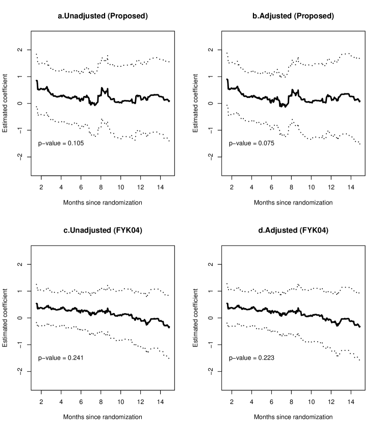
Figure 2: Plots for the estimated regression coefficients of treatment effect along with the 95% simultaneous confidence bands and the p-values based on the nonparametric tests for the tumor response state: (a) Unadjusted treatment effect based on the proposed method; (b) Adjusted treatment effect based on the proposed method; (c) Unadjusted treatment effect based on the method proposed by Fine et al. (2004) (FYK04) for independent observations; (d) Adjusted treatment effect based on the FYK04 for independent observations.

The estimated time-varying regression parameters for treatment (chemotherapy + panitumumab vs chemotherapy alone) along with the corresponding 95% simultaneous confidence bands and the p-values (based on the proposed Kolmogorov–Smirnov-type tests) are presented in Figure 2. For comparison, Figure 2 also includes the results from the analysis that ignores the within-cluster dependence and the ICS (Fine et al., 2004). Based on the proposed method, being in the panitumumab plus chemotherapy arm was associated with a higher probability of being in the ”tumor response” state over time compared to the chemotherapy alone arm, conditionally on being alive. However, the unadjusted treatment effect was not statistically significant. After adjusting for the stratification variables and other potentially important baseline covariates (i.e., sex, ECOG performance status, prior treatment history, site of primary tumor, race, and age), the treatment effect became marginally significant (p-value=0.075). This indicates an efficiency increase as a result of adjusting for the stratification variables and other covariates. The analysis based on the previously proposed method (Fine et al., 2004) provided somewhat less pronounced treatment effects, and this may be an indication of ICS. The 95% simultaneous confidence bands from the latter approach were narrower compared to those from the proposed method, which is attributed to under-estimated standard errors as a consequence of ignoring the within-cluster dependence.

The p-values for the remaining covariate effects in the adjusted model from the proposed method and the previously proposed method (Fine et al., 2004) are summarized in Table 5. Plots for the estimated time-varying regression coefficients, along with the corresponding 95% simultaneous confidence bands and the p-values, are provided in the Supplementary Material. Based on the proposed method, the effects of sex and age on the state occupation probability of the tumor response state, conditionally on being alive, were statistically significant. In contrast, none of the covariate effects were statistically significant based on the previously proposed method for independent observations, which may be attributed to a potential ICS.

5 Discussion

In this paper, we addressed the issue of marginal regression analysis of transient state occupation probabilities with right-censored multistate process data with cluster-correlated observations, allowing also for ICS. To achieve this, we proposed a weighted functional generalized estimating equations approach. Rigorous methods for computing simultaneous confidence bands and a nonparametric hypothesis testing procedure for covariate effects were also proposed. Our methodology does not impose assumptions regarding the within-cluster dependence and does not require the Markov assumption. The validity of our methodology was justified both theoretically and via extensive simulation experiments. The latter experiments showed that ignoring the within-cluster dependence and the ICS can lead to invalid inferences. This highlights the practical importance of the proposed methodology in settings with clustered multistate processes and potential ICS. Software in the form of R code, together with a sample input data set and complete documentation, are available per request from the first author (wz11@iu.edu).

The issue of marginal analysis of clustered and right-censored multistate process data has received some attention in the recent literature. Bakoyannis (2021) proposed a nonparametric moment-based estimator and a two-sample Kolmogorov-Smirnov-type test for state occupation and transition probabilities. Bakoyannis and Bandyopadhyay (2022) proposed additional nonparametric two-sample tests for this problem, which may be more powerful than the Kolmogorov-Smirnov-type test for certain alternative hypotheses. Even though these methods allow for ICS, they do not incorporate covariates. To the best of our knowledge, there was no method for marginal regression on transient state occupation probabilities for clustered and right-censored multistate process data prior to this work. Nevertheless, the problem of regression analysis of clustered multistate data is crucial in many applications, such as in our motivating SPECTRUM trial (Vermorken et al., 2013). The analysis of the data from the latter trial illustrated that, ignoring the within-cluster dependence and the potential ICS may lead to substantially biased inferences in practice.

In situations with ICS, two populations are typically of interest: the population of all cluster members (ACM) and the population of typical cluster members (TCM) (Seaman et al., 2014). The ACM population includes all observations from all clusters, while the TCM population is comprised of a randomly selected observation from each cluster. As a consequence, the larger clusters dominate the ACM population, while all clusters are equally represented in the TCM population. The choice of the most appropriate target population in a given study depends on the scientific question under investigation. More details about the practical relevance of the two populations can be found in the articles by Bakoyannis (2021) and Bakoyannis and Bandyopadhyay (2022). In this work, the proposed methodology provides inferences for the TCM population, in an effort to adjust for the over-representation of larger clusters. However, in some applications, the ACM population may be more scientifically relevant, such as in public health and health policy studies. In such cases, the proposed methodology can be easily modified to provide inferences for the ACM population by simply removing the weight $1/M_{i}$ from the weighted functional generalized estimating equations and the empirical versions of the influence functions.

There is a number of possible extensions to this work. For example, extending the methodology to incorporate incompletely observed covariates is both methodologically interesting and scientifically relevant in many studies (Chen et al., 2012). Another useful but challenging extension would be to relax the i.i.d. assumption across clusters and allow, for example, some dependence between clusters in close spatial proximity (e.g., hospitals from the same region).

Funding

This research was supported in part by the National Institutes Health grant number R21AI145662 and Lilly Endowment, Inc., through its support for the Indiana University Pervasive Technology Institute.

Supplement

Supplementary Material A

Proofs of Theorem 1, Theorem 2 and explicit formulas for the empirical versions of the influence functions referred in Section 2 are provided in Supplementary Material A.

Supplementary Material B

Additional simulation results and data analysis results referred in Section 3 and Section 4 are provided in Supplementary Material B.

Table 1: Pointwise simulation results for the estimated functional regression parameters $\hat{\beta}_{n,2,1}(\cdot)$ based on the proposed approach and the approach by Fine et al. (2004) (FYK04) for independent observations.

		Proposed				FYK04
$n$	$t$	Bias	ASE	MCSD	CP	Bias	ASE	MCSD	CP
50	0.2	-0.003	0.053	0.057	0.924	-0.013	0.040	0.057	0.818
	0.4	-0.003	0.056	0.058	0.940	-0.013	0.043	0.057	0.855
	0.6	-0.003	0.058	0.062	0.928	-0.014	0.045	0.062	0.845
	0.8	-0.005	0.061	0.064	0.935	-0.015	0.048	0.063	0.862
	1.0	-0.004	0.063	0.069	0.924	-0.015	0.050	0.068	0.840
	1.2	-0.004	0.065	0.071	0.924	-0.015	0.053	0.068	0.861
	1.4	-0.007	0.067	0.073	0.926	-0.017	0.055	0.072	0.862
	1.6	-0.004	0.070	0.076	0.916	-0.015	0.057	0.074	0.870
	1.8	-0.004	0.072	0.078	0.915	-0.015	0.059	0.075	0.872
100	0.2	-0.002	0.038	0.038	0.944	-0.013	0.028	0.038	0.822
	0.4	-0.002	0.040	0.041	0.950	-0.013	0.030	0.040	0.834
	0.6	-0.004	0.042	0.041	0.946	-0.015	0.032	0.041	0.843
	0.8	-0.004	0.044	0.043	0.956	-0.015	0.034	0.043	0.863
	1.0	-0.005	0.045	0.046	0.949	-0.015	0.035	0.045	0.865
	1.2	-0.005	0.047	0.048	0.941	-0.016	0.037	0.047	0.863
	1.4	-0.005	0.048	0.048	0.958	-0.015	0.038	0.047	0.880
	1.6	-0.005	0.050	0.050	0.938	-0.015	0.040	0.049	0.884
	1.8	-0.005	0.051	0.053	0.944	-0.016	0.041	0.052	0.880
200	0.2	-0.002	0.027	0.027	0.952	-0.013	0.020	0.027	0.818
	0.4	-0.002	0.028	0.028	0.951	-0.013	0.021	0.027	0.831
	0.6	-0.002	0.030	0.030	0.949	-0.013	0.022	0.029	0.824
	0.8	-0.001	0.031	0.032	0.936	-0.012	0.024	0.031	0.840
	1.0	-0.001	0.032	0.032	0.947	-0.012	0.025	0.032	0.845
	1.2	-0.002	0.033	0.035	0.935	-0.013	0.026	0.034	0.835
	1.4	-0.002	0.034	0.034	0.951	-0.013	0.027	0.034	0.869
	1.6	-0.002	0.036	0.036	0.947	-0.013	0.028	0.035	0.860
	1.8	-0.002	0.037	0.037	0.941	-0.012	0.029	0.036	0.880
400	0.2	-0.001	0.019	0.018	0.969	-0.011	0.014	0.018	0.795
	0.4	-0.001	0.020	0.020	0.943	-0.011	0.015	0.020	0.799
	0.6	-0.001	0.021	0.021	0.950	-0.012	0.016	0.021	0.799
	0.8	-0.001	0.022	0.022	0.942	-0.012	0.017	0.022	0.797
	1.0	-0.001	0.023	0.023	0.941	-0.013	0.017	0.023	0.825
	1.2	-0.001	0.024	0.022	0.968	-0.012	0.018	0.022	0.851
	1.4	-0.001	0.024	0.024	0.958	-0.013	0.019	0.024	0.833
	1.6	-0.001	0.025	0.025	0.958	-0.012	0.020	0.024	0.834
	1.8	-0.002	0.026	0.025	0.949	-0.013	0.021	0.025	0.849

Note: $n$: number of clusters with the cluster size $M\in\{20,\ldots,60\}$; ASE: average estimated standard error; MCSD: Monte Carlo standard deviation of the estimates; CP: coverage probability of $95\%$ pointwise confidence interval.

Table 2: Simulation results for the coverage probabilities of the $95\%$ simultaneous confidence bands for the proposed method and the method by Fine et al. (2004) (FYK04) for independent observations.

	Proposed			FYK04
$n$	$\beta_{0,2,0}(t)$	$\beta_{0,2,1}(t)$	$\beta_{0,2,2}(t)$	$\beta_{0,2,0}(t)$	$\beta_{0,2,1}(t)$	$\beta_{0,2,2}(t)$
50	0.921	0.899	0.883	0.221	0.813	0.722
100	0.932	0.929	0.933	0.143	0.801	0.704
200	0.943	0.941	0.934	0.067	0.795	0.672
400	0.949	0.948	0.954	0.006	0.776	0.640

Note: $n$: number of clusters with the cluster size $M\in\{20,\ldots,60\}$.

Table 3: Simulation results on the empirical type I error rates $(H_{0})$ and the power levels $(H_{1})$ for the proposed Kolmogorov–Smirnov-test and the corresponding test proposed by Fine et al. (2004) (FYK04) for independent observations, at the $\alpha=0.05$ level.

	Proposed		FYK04
$n$	$\beta_{0,2,1}(t)$	$\beta_{0,2,2}(t)$	$\beta_{0,2,1}(t)$	$\beta_{0,2,2}(t)$
$H_{0}:\beta_{0,2,l}(t)=0,\quad l=1,2$
50	0.085	0.081	0.110	0.180
100	0.084	0.067	0.133	0.187
200	0.047	0.059	0.137	0.201
400	0.047	0.057	0.125	0.201
$H_{1}:\beta_{0,2,l}(t)=-0.05,\quad l=1,2$
50	0.297	0.388	0.415	0.608
100	0.444	0.610	0.641	0.838
200	0.714	0.861	0.887	0.976
400	0.930	0.991	0.991	1.000
$H_{1}:\beta_{0,2,l}(t)=-0.1,\quad l=1,2$
50	0.699	0.843	0.857	0.958
100	0.931	0.987	0.983	1.000
200	0.997	1.000	1.000	1.000
400	1.000	1.000	1.000	1.000
$H_{1}:\beta_{0,2,l}(t)=-0.25,\quad l=1,2$
50	0.999	0.998	1.000	1.000
100	1.000	1.000	1.000	1.000
200	1.000	1.000	1.000	1.000
400	1.000	1.000	1.000	1.000

Note: $n$: number of clusters with the cluster size $M\in\{20,\ldots,60\}$.

Table 4: SPECTRUM trial data analysis: Descriptive characteristics of the analysis sample.

Variable	Panitumumab $+$ Chemotherapy	Chemotherapy Alone	Overall
	($N$=260)	($N$=260)	($N$=520)
	$n$ (%)	$n$ (%)	$n$ (%)
Sex
Male	227 (87.3)	228 (87.7)	455 (87.5)
Female	33 (12.7)	32 (12.3)	65 (12.5)
ECOG performance status
Fully active	190 (73.1)	180 (69.2)	370 (71.2)
Other	70 (26.9)	80 (30.8)	150 (28.8)
Prior treatment history
Recurrent	206 (79.2)	201 (77.3)	407 (78.3)
Newly diagnosed	54 (20.8)	59 (22.7)	113 (21.7)
Site of primary tumor
Oropharynx/ Larynx	154 (59.2)	149 (57.3)	303 (58.3)
Hypopharynx/ Oral cavity	106 (40.8)	111 (42.7)	217 (41.7)
Race
White or Caucasian	236 (90.8)	230 (88.5)	466 (89.6)
Other	24 (9.2)	30 (11.5)	54 (10.4)
	Median (IQR)	Median (IQR)	Median (IQR)
Age1	58.0 (53.0, 62.0)	58.5 (53.0, 63.0)	58.0 (53.0, 63.0)

Note: ¹: Age in years at screening.

Table 5: SPECTRUM trial data analysis: p-values for the functional covariate effects for the tumor response state based on the proposed Kolmogorov–Smirnov-test and the corresponding test proposed by Fine et al. (2004) (FYK04) for independent observations.

Variable	Proposed	FYK04
Treatment (panitumumab + chemotherapy = 1, chemotherapy alone = 0)	0.075	0.223
Sex (male = 1, female = 0)	0.011	0.180
ECOG performance status (fully active = 1, other = 0)	0.251	0.361
Prior treatment history (recurrent = 1, newly diagnosed = 0)	0.271	0.159
Site of primary tumor (oropharynx/larynx = 1, hypopharynx/ oral cavity = 0)	0.630	0.632
Race (White or Caucasian = 1, other = 0)	0.518	0.878
Age1 (per year)	0.044	0.775

Note: ¹: Age in years at screening.

Appendix A Asymptotic Theory Proofs

We justify the asymptotic properties of the proposed estimators using empirical process theory techniques (Kosorok, 2008; van der Vaart and Wellner, 1996). In this section, we provide the proofs for Theorems 2.1 and 2.2, and the explicit formulas for the empirical versions of the influence functions. For notational simplicity, we omit the subscript $h$, indicating the transient state of interest, from the proofs.

A.1 Proof of Theorem 2.1

We first define

$$\boldsymbol{C}_{i}(\boldsymbol{\gamma},\boldsymbol{\beta},{t})=\frac{1}{M_{i}}\sum_{j=1}^{M_{i}}{S}_{ij}(t){R}_{ij}(t)\boldsymbol{D}_{ij}^{T}\left[\boldsymbol{\gamma}(t)\right]{V}_{ij}\left[\boldsymbol{\gamma}(t),{t}\right]\left\{\tilde{Y}_{ij}(t)-f\left[\boldsymbol{\beta}^{T}(t){X}_{ij}(t)\right]\right\},$$

with $f=g^{-1}$ and $\boldsymbol{\gamma},\boldsymbol{\beta}\in\left\{l_{c}^{\infty}[0,\tau]\right\}^{p}$, where $\{l_{c}^{\infty}[0,\tau]\}^{p}$ denotes the space of bounded vector-valued real functions defined on $[0,\tau]$ with absolute value bounded above by $c$. We omit the subindex $i$ and use the notation $\boldsymbol{C}(\boldsymbol{\gamma},\boldsymbol{\beta},{t})$ to denote the generic version of the random quanity $\boldsymbol{C}_{i}(\boldsymbol{\gamma},\boldsymbol{\beta},{t})$ for an arbitrary cluster. We first argue that the class of functions

$$\mathcal{L}=\left\{\boldsymbol{C}(\boldsymbol{\gamma},\boldsymbol{\beta},{t}):\boldsymbol{\gamma},\boldsymbol{\beta}\in\left\{l_{c}^{\infty}[0,\tau]\right\}^{p},t\in[0,\tau]\right\},$$

is Donsker. By condition C3 we have that

$$\boldsymbol{C}(\boldsymbol{\gamma},\boldsymbol{\beta},{t}) = \sum_{j=1}^{m_{0}}\frac{1}{M}I(M\geq j){S}_{j}(t){R}_{j}(t)\boldsymbol{D}_{j}^{T}\left[\boldsymbol{\gamma}(t)\right]{V}_{j}\left[\boldsymbol{\gamma}(t),{t}\right]\left\{\tilde{Y}_{j}(t)-f\left[\boldsymbol{\beta}^{T}(t){X}_{j}(t)\right]\right\}$$ (4)

$$\equiv \sum_{j=1}^{m_{0}}\frac{1}{M}I(M\geq j)\tilde{\boldsymbol{C}}_{j}(\boldsymbol{\gamma},\boldsymbol{\beta},{t}).$$

Under conditions C1, C2, and C4-C6, and using arguments similar to those used in the proof of Theorem A1 in Fine et al. (2004), it follows that the classes of functions

$$\left\{\tilde{\boldsymbol{C}}_{j}(\boldsymbol{\gamma},\boldsymbol{\beta},{t}):\boldsymbol{\gamma},\boldsymbol{\beta}\in\{l_{c}^{\infty}[0,\tau]\}^{p},t\in[0,\tau]\right\},\ \ \ \ j=1,\ldots,m_{0},$$

are Donsker. This result along with the fact that $E[M^{-1}I(M\geq j)]^{2}\leq 1$, $j=1,\ldots m_{0}$, and (4), lead to the conclusion that the class $\mathcal{L}$ is also Donsker, since (finite) sums of products of Donsker classes with random variables with bounded second moments are Donsker. In addition to this result, we need to show that the proposed estimating equation is unbiased, that is

$$E[\boldsymbol{C}(\tilde{\boldsymbol{\beta}},\boldsymbol{\beta}_{0},t)]=\boldsymbol{0},$$

for all $\tilde{\boldsymbol{\beta}}\in\{l_{c}^{\infty}[0,\tau]\}^{p}$ and $t\in[0,\tau]$. By conditions C1, C3, C7, and the missing at random (MAR) assumption imposed in Section 2.1, we have, for all $\tilde{\boldsymbol{\beta}}\in\{l_{c}^{\infty}[0,\tau]\}^{p}$ and $t\in[0,\tau]$, that

$$E\left[\boldsymbol{C}(\boldsymbol{\tilde{\beta}},\boldsymbol{\beta}_{0},t)\right]$$

$$= E\left[\frac{1}{M}\sum_{j=1}^{m_{0}}I(M\geq j)S_{j}(t)R_{j}(t)\boldsymbol{D}_{j}^{T}\left[\boldsymbol{\tilde{\beta}}(t)\right]V_{j}\left[\boldsymbol{\tilde{\beta}}(t),t\right]\left\{\tilde{Y}_{j}(t)-f\left[\boldsymbol{\beta}_{0}^{T}(t)\boldsymbol{X}_{j}(t)\right]\right\}\right]$$

$$= E\left\{\frac{1}{M}\sum_{j=1}^{m_{0}}I(M\geq j)E\left[S(t)R(t)\boldsymbol{D}^{T}\left[\boldsymbol{\tilde{\beta}}(t)\right]V\left[\boldsymbol{\tilde{\beta}}(t),t\right]\left\{\tilde{Y}(t)-f\left[\left.\boldsymbol{\beta}_{0}^{T}(t)\boldsymbol{X}(t)\right]\right\}\right|M\right]\right\}$$

$$= E\left\{E\left[\left.S(t)R(t)\boldsymbol{D}^{T}\left[\boldsymbol{\tilde{\beta}}(t)\right]V\left[\boldsymbol{\tilde{\beta}}(t),t\right]\left\{\tilde{Y}(t)-f\left[\boldsymbol{\beta}_{0}^{T}(t)\boldsymbol{X}(t)\right]\right\}\right|M\right]\frac{1}{M}\sum_{j=1}^{m_{0}}I(M\geq j)\right\}$$

$$= E\left\{E\left[\left.S(t)R(t)\boldsymbol{D}^{T}\left[\boldsymbol{\tilde{\beta}}(t)\right]V\left[\boldsymbol{\tilde{\beta}}(t),t\right]\left\{\tilde{Y}(t)-f\left[\boldsymbol{\beta}_{0}^{T}(t)\boldsymbol{X}(t)\right]\right\}\right|M\right]\right\}$$

$$= E\left[S(t)R(t)\boldsymbol{D}^{T}\left[\boldsymbol{\tilde{\beta}}(t)\right]V\left[\boldsymbol{\tilde{\beta}}(t),t\right]\left\{\tilde{Y}(t)-f\left[\boldsymbol{\beta}_{0}^{T}(t)\boldsymbol{X}(t)\right]\right\}\right]$$

$$= E\left\{E\left[\left.S(t)R(t)\boldsymbol{D}^{T}\left[\boldsymbol{\tilde{\beta}}(t)\right]{V}\left[\boldsymbol{\tilde{\beta}}(t),t\right]\left\{\tilde{Y}(t)-f\left[\boldsymbol{\beta}_{0}^{T}(t)\boldsymbol{X}(t)\right]\right\}\right|\boldsymbol{X}(t),S(t)=1\right]\right\}$$

$$= E\left[\boldsymbol{D}^{T}\left[\boldsymbol{\tilde{\beta}}(t)\right]V\left[\boldsymbol{\tilde{\beta}}(t),{t}\right]E\left[R(t)|\boldsymbol{X}(t),S(t)=1\right]\left\{E\left[\left.\tilde{Y}(t)\right|\boldsymbol{X}(t),S(t)=1\right]-f\left[\boldsymbol{\beta}_{0}^{T}(t)\boldsymbol{X}(t)\right]\right\}\right]$$

$$= \boldsymbol{0}.$$

These facts and arguments similar to those used in the proof of Theorem A1 in Fine et al. (2004) conclude the proof of Theorem 2.1.

A.2 Proof of Theorem 2.2

By definition, the proposed estimator satisfies

$$\boldsymbol{0} = n^{-1/2}\boldsymbol{U}[\boldsymbol{\hat{\beta}}_{n}(t),t]$$

$$= n^{-1/2}\boldsymbol{U}\left[\boldsymbol{\beta}_{0}(t),t\right]+n^{-1/2}\left\{\boldsymbol{U}[\boldsymbol{\hat{\beta}}_{n}(t),t]-\boldsymbol{U}\left[\boldsymbol{\beta}_{0}(t),t\right]\right\}$$

$$= n^{-1/2}\boldsymbol{U}\left[\boldsymbol{\beta}_{0}(t),t\right]+n^{-1/2}\sum_{i=1}^{n}\left[\boldsymbol{C}_{i}(\boldsymbol{\hat{\beta}}_{n},\boldsymbol{\beta}_{0},t)-\boldsymbol{C}_{i}(\boldsymbol{\beta}_{0},\boldsymbol{\beta}_{0},t)\right]$$

$$+n^{-1/2}\sum_{i=1}^{n}\frac{1}{M_{i}}\sum_{j=1}^{M_{i}}S_{ij}(t)R_{ij}(t)\boldsymbol{D}_{ij}^{T}[\boldsymbol{\hat{\beta}}_{n}(t)]V_{ij}[\boldsymbol{\hat{\beta}}_{n}(t),t]\left\{f[\boldsymbol{\hat{\beta}}_{n}^{T}(t)\boldsymbol{X}_{ij}(t)]-f[\boldsymbol{\beta}_{0}^{T}(t)\boldsymbol{X}_{ij}(t)]\right\}$$

$$= \boldsymbol{U}_{0}(t)+\boldsymbol{U}_{1}(t)+\boldsymbol{U}_{2}(t)$$

We will first argue that the $\sup_{t\in[0,\tau]}\|\boldsymbol{U}_{1}(t)\|\overset{p}{\rightarrow}0$. First, note that the class of functions

$$\left\{\boldsymbol{C}(\boldsymbol{\beta},\boldsymbol{\beta}_{0},{t})-\boldsymbol{C}(\boldsymbol{\beta}_{0},\boldsymbol{\beta}_{0},{t}):\boldsymbol{\beta}\in\left\{l_{c}^{\infty}[0,\tau]\right\}^{p},\sup_{t\in[0,\tau]}\|\boldsymbol{\beta}(t)-\boldsymbol{\beta}_{0}(t)\|<\delta,t\in[0,\tau]\right\}$$

is Donsker for some $\delta>0$, because it is formed by the difference between two classes which are subsets of the Donsker class $\mathcal{L}$. Next, let $C^{(l)}(\boldsymbol{\beta},\boldsymbol{\beta}_{0},t)$ denote the $(l+1)th$ component of $\boldsymbol{C}(\boldsymbol{\beta},\boldsymbol{\beta}_{0},{t})$, $l=0,\ldots,p$, and $D_{j}^{(l)}(\boldsymbol{\beta}(t))$ be the $(l+1)th$ component of $\boldsymbol{D}_{j}(\boldsymbol{\beta}(t))$, $j=1,\ldots,m_{0}$. Under conditions C2-C4 and C6, and for any $t\in[0,\tau]$, we have that

$$E\left[C^{(l)}(\boldsymbol{\beta},\boldsymbol{\beta}_{0},t)-C^{(l)}(\boldsymbol{\beta}_{0},\boldsymbol{\beta}_{0},t)\right]^{2} \leq E\left[\sum_{j=1}^{m_{0}}\left|D_{j}^{(l)}(\boldsymbol{\beta}(t))V_{j}(\boldsymbol{\beta}(t),t)-D_{j}^{(l)}(\boldsymbol{\beta}_{0}(t))V_{j}(\boldsymbol{\beta}_{0}(t),t)\right|\right]^{2}$$

$$\leq m_{0}^{2}E\left[\max_{1\leq j\leq m_{0}}\left|D_{j}^{(l)}(\boldsymbol{\beta}(t))V_{j}(\boldsymbol{\beta}(t),t)-D_{j}^{(l)}(\boldsymbol{\beta}_{0}(t))V_{j}(\boldsymbol{\beta}_{0}(t),t)\right|\right]^{2}$$

$$\leq \|\boldsymbol{\beta}(t)-\boldsymbol{\beta}_{0}(t)\|^{2}m_{0}^{2}K^{2},\ \ \ \ l=0,\ldots,p,$$

where $K<\infty$ is the supremum of the set of Lipschitz constants of the functions $\boldsymbol{\beta}(t)\mapsto D_{j}^{(l)}(\boldsymbol{\beta}(t))V_{j}(\boldsymbol{\beta}(t),t)$ for any covariate pattern in the covariate space and $t\in[0,\tau]$. This implies that

$$\sup_{t\in[0,\tau]}E\left[C^{(l)}(\boldsymbol{\beta},\boldsymbol{\beta}_{0},t)-C^{(l)}(\boldsymbol{\beta}_{0},\boldsymbol{\beta}_{0},t)\right]^{2}\rightarrow 0,\ \ \ \ l=0,\ldots,p,$$

as $\sup_{t\in[0,\tau]}\|\boldsymbol{\beta}(t)-\boldsymbol{\beta}_{0}(t)\|\rightarrow 0$. The latter two results along with Theorem 2.1 and arguments similar to those used in the proof of Lemma 3.3.5. in van der Vaart and Wellner (1996) lead to the conclusion that

$$\sup_{t\in[0,\tau]}\left\|\boldsymbol{U}_{1}(t)\right\|\overset{p}{\rightarrow}0.$$

This result and arguments similar to those used in the proofs of theorems A2 and A3 in Fine et al. (2004) conclude the proof of Theorem 2.2.

Appendix B Additional numerical Results

B.1 Additional Simulation Results

Simulation results for the pointwise estimates of the regression parameters $\beta_{0,2,2}$ and $\beta_{0,2,0}$ are provided in Table 6 and Table 7, respectively.

Table 6: Pointwise simulation results for the estimated functional regression parameters $\hat{\beta}_{n,2,2}(\cdot)$ based on the proposed approach and the approach by Fine et al. (2004) (FYK04) for independent observations.

		Proposed				FYK04
$n$	$t$	Bias	ASE	MCSD	CP	Bias	ASE	MCSD	CP
50	0.2	-0.005	0.046	0.047	0.924	-0.016	0.029	0.048	0.762
	0.4	-0.005	0.048	0.052	0.922	-0.015	0.032	0.052	0.766
	0.6	-0.006	0.05	0.052	0.918	-0.017	0.034	0.053	0.795
	0.8	-0.005	0.052	0.055	0.925	-0.015	0.036	0.055	0.782
	1.0	-0.006	0.054	0.057	0.922	-0.016	0.038	0.057	0.791
	1.2	-0.006	0.056	0.061	0.916	-0.017	0.040	0.060	0.807
	1.4	-0.007	0.058	0.063	0.933	-0.017	0.042	0.062	0.805
	1.6	-0.006	0.059	0.066	0.911	-0.016	0.043	0.065	0.830
	1.8	-0.005	0.061	0.064	0.923	-0.015	0.045	0.064	0.835
100	0.2	-0.003	0.033	0.033	0.951	-0.013	0.021	0.033	0.728
	0.4	-0.003	0.034	0.036	0.946	-0.013	0.022	0.035	0.763
	0.6	-0.003	0.035	0.036	0.946	-0.013	0.024	0.036	0.785
	0.8	-0.003	0.037	0.039	0.945	-0.014	0.025	0.039	0.768
	1.0	-0.004	0.039	0.040	0.944	-0.014	0.027	0.040	0.793
	1.2	-0.004	0.040	0.041	0.939	-0.014	0.028	0.040	0.792
	1.4	-0.004	0.041	0.042	0.944	-0.014	0.029	0.042	0.818
	1.6	-0.004	0.042	0.044	0.945	-0.014	0.030	0.043	0.823
	1.8	-0.004	0.043	0.045	0.932	-0.014	0.032	0.045	0.822
200	0.2	-0.002	0.023	0.023	0.945	-0.013	0.014	0.024	0.719
	0.4	-0.003	0.024	0.024	0.947	-0.013	0.016	0.024	0.744
	0.6	-0.002	0.025	0.026	0.950	-0.013	0.017	0.025	0.758
	0.8	-0.003	0.026	0.027	0.940	-0.014	0.018	0.027	0.774
	1.0	-0.002	0.027	0.028	0.949	-0.013	0.019	0.027	0.782
	1.2	-0.002	0.028	0.029	0.939	-0.013	0.020	0.029	0.774
	1.4	-0.003	0.029	0.030	0.944	-0.014	0.021	0.030	0.782
	1.6	-0.004	0.030	0.031	0.942	-0.014	0.021	0.031	0.806
	1.8	-0.004	0.031	0.032	0.942	-0.014	0.022	0.032	0.788
400	0.2	-0.001	0.016	0.016	0.961	-0.012	0.010	0.016	0.685
	0.4	-0.001	0.017	0.017	0.960	-0.012	0.011	0.017	0.689
	0.6	-0.002	0.018	0.018	0.958	-0.013	0.012	0.018	0.718
	0.8	-0.001	0.019	0.019	0.948	-0.013	0.013	0.018	0.706
	1.0	-0.001	0.019	0.019	0.961	-0.013	0.013	0.019	0.735
	1.2	-0.002	0.020	0.020	0.941	-0.013	0.014	0.020	0.742
	1.4	-0.002	0.021	0.020	0.955	-0.013	0.014	0.020	0.760
	1.6	-0.002	0.021	0.022	0.942	-0.013	0.015	0.021	0.758
	1.8	-0.002	0.022	0.022	0.949	-0.013	0.016	0.021	0.778

Note: $n$: number of clusters with cluster size $M\in\{20,\ldots,60\}$; ASE: average estimated standard error; MCSD: Monte Carlo standard deviation of the estimates; CP: coverage probability of $95\%$ pointwise confidence interval.

Table 7: Pointwise simulation results for the estimated functional regression parameters $\hat{\beta}_{n,2,0}(\cdot)$ based on the proposed approach and the approach by Fine et al. (2004) (FYK04) for independent observations.

		Proposed				FYK04
$n$	$t$	Bias	ASE	MCSD	CP	Bias	ASE	MCSD	CP
50	0.2	-0.013	0.254	0.253	0.952	0.225	0.074	0.257	0.284
	0.4	-0.012	0.258	0.261	0.950	0.241	0.084	0.262	0.294
	0.6	0.000	0.267	0.270	0.944	0.261	0.095	0.270	0.314
	0.8	0.000	0.276	0.282	0.946	0.266	0.105	0.280	0.357
	1.0	0.001	0.287	0.297	0.938	0.270	0.115	0.293	0.375
	1.2	0.003	0.296	0.311	0.930	0.278	0.125	0.306	0.379
	1.4	0.009	0.307	0.328	0.926	0.286	0.134	0.323	0.402
	1.6	0.009	0.315	0.337	0.929	0.289	0.143	0.330	0.426
	1.8	0.002	0.325	0.345	0.929	0.283	0.152	0.338	0.458
100	0.2	0.000	0.179	0.183	0.948	0.240	0.051	0.183	0.185
	0.4	0.002	0.182	0.192	0.941	0.257	0.059	0.190	0.201
	0.6	0.006	0.189	0.199	0.938	0.270	0.067	0.196	0.217
	0.8	0.009	0.196	0.205	0.934	0.279	0.074	0.202	0.222
	1.0	0.013	0.204	0.217	0.928	0.287	0.081	0.212	0.247
	1.2	0.011	0.210	0.224	0.933	0.289	0.087	0.218	0.259
	1.4	0.015	0.218	0.233	0.935	0.298	0.094	0.228	0.286
	1.6	0.014	0.224	0.240	0.934	0.298	0.100	0.235	0.313
	1.8	0.013	0.231	0.246	0.929	0.299	0.106	0.242	0.326
200	0.2	-0.005	0.127	0.130	0.944	0.236	0.036	0.133	0.096
	0.4	-0.001	0.129	0.131	0.943	0.255	0.042	0.132	0.095
	0.6	-0.003	0.134	0.136	0.944	0.262	0.047	0.136	0.097
	0.8	0.002	0.139	0.144	0.938	0.273	0.052	0.143	0.113
	1.0	0.000	0.145	0.147	0.952	0.277	0.057	0.146	0.123
	1.2	0.002	0.150	0.154	0.943	0.282	0.061	0.151	0.146
	1.4	0.004	0.155	0.155	0.959	0.287	0.066	0.153	0.149
	1.6	0.005	0.160	0.166	0.940	0.291	0.070	0.163	0.163
	1.8	0.007	0.164	0.171	0.945	0.294	0.075	0.169	0.186
400	0.2	0.000	0.090	0.089	0.957	0.240	0.026	0.091	0.016
	0.4	0.002	0.091	0.090	0.950	0.258	0.029	0.091	0.018
	0.6	0.004	0.095	0.093	0.956	0.268	0.033	0.093	0.014
	0.8	0.004	0.099	0.098	0.947	0.275	0.037	0.097	0.018
	1.0	0.006	0.102	0.102	0.945	0.282	0.040	0.100	0.016
	1.2	0.007	0.106	0.104	0.944	0.286	0.043	0.103	0.029
	1.4	0.007	0.110	0.108	0.949	0.291	0.047	0.107	0.027
	1.6	0.006	0.113	0.113	0.950	0.292	0.050	0.112	0.032
	1.8	0.008	0.117	0.114	0.955	0.296	0.053	0.113	0.038

Note: $n$: number of clusters with cluster size $M\in\{20,\ldots,60\}$; ASE: average estimated standard error; MCSD: Monte Carlo standard deviation of the estimates; CP: coverage probability of $95\%$ pointwise confidence interval.

Additional simulation results under a more variable cluster size $M\in\{5,\ldots,105\}$ are presented in Tables 8-12.

Table 8: Pointwise simulation results for the estimated functional regression parameters $\hat{\beta}_{n,2,0}(\cdot)$ based on the proposed approach and the approach by Fine et al. (2004) (FYK04) for independent observations. Simulation scenario with a more variable cluster size $M\in\{5,\ldots,105\}$.

		Proposed				FYK04
$n$	$t$	Bias	ASE	MCSD	CP	Bias	ASE	MCSD	CP
50	0.2	-0.011	0.255	0.256	0.946	0.456	0.065	0.276	0.101
	0.4	-0.003	0.260	0.264	0.947	0.513	0.078	0.274	0.086
	0.6	0.000	0.270	0.280	0.948	0.545	0.089	0.284	0.083
	0.8	0.011	0.282	0.292	0.929	0.578	0.100	0.293	0.080
	1.0	0.015	0.293	0.305	0.943	0.600	0.111	0.302	0.099
	1.2	0.016	0.305	0.327	0.936	0.620	0.121	0.315	0.098
	1.4	0.017	0.314	0.341	0.927	0.631	0.131	0.326	0.119
	1.6	0.013	0.326	0.343	0.937	0.644	0.140	0.336	0.127
	1.8	0.014	0.337	0.358	0.935	0.654	0.150	0.345	0.138
100	0.2	-0.004	0.180	0.186	0.947	0.468	0.046	0.195	0.025
	0.4	0.001	0.184	0.194	0.946	0.523	0.054	0.197	0.012
	0.6	0.008	0.192	0.204	0.937	0.560	0.062	0.203	0.012
	0.8	0.011	0.200	0.212	0.934	0.587	0.070	0.209	0.015
	1.0	0.014	0.209	0.220	0.933	0.611	0.077	0.216	0.017
	1.2	0.018	0.217	0.231	0.927	0.627	0.085	0.225	0.018
	1.4	0.017	0.224	0.240	0.928	0.641	0.091	0.229	0.016
	1.6	0.014	0.232	0.247	0.927	0.651	0.098	0.237	0.018
	1.8	0.021	0.240	0.256	0.931	0.668	0.104	0.243	0.022
200	0.2	-0.004	0.127	0.129	0.954	0.469	0.032	0.138	0.004
	0.4	-0.002	0.130	0.132	0.955	0.521	0.038	0.138	0.000
	0.6	-0.003	0.136	0.137	0.947	0.555	0.044	0.140	0.000
	0.8	-0.001	0.142	0.144	0.948	0.581	0.049	0.145	0.000
	1.0	0.003	0.148	0.148	0.950	0.602	0.055	0.150	0.000
	1.2	0.002	0.154	0.157	0.936	0.618	0.059	0.156	0.000
	1.4	0.001	0.160	0.165	0.946	0.634	0.064	0.163	0.000
	1.6	-0.002	0.165	0.169	0.939	0.641	0.069	0.166	0.000
	1.8	0.001	0.171	0.176	0.944	0.656	0.073	0.168	0.000
400	0.2	0.002	0.090	0.088	0.951	0.471	0.023	0.095	0.000
	0.4	0.002	0.092	0.091	0.957	0.522	0.027	0.096	0.000
	0.6	0.003	0.096	0.095	0.958	0.556	0.031	0.097	0.000
	0.8	0.006	0.101	0.098	0.955	0.584	0.035	0.100	0.000
	1.0	0.008	0.105	0.107	0.946	0.606	0.039	0.104	0.000
	1.2	0.006	0.109	0.109	0.949	0.620	0.042	0.108	0.000
	1.4	0.006	0.113	0.112	0.949	0.636	0.045	0.110	0.000
	1.6	0.006	0.117	0.114	0.966	0.647	0.049	0.110	0.000
	1.8	0.007	0.121	0.119	0.948	0.659	0.052	0.113	0.000

Note: $n$: number of clusters with cluster size $M\in\{5,\ldots,105\}$; ASE: average estimated standard error; MCSD: Monte Carlo standard deviation of the estimates; CP: coverage probability of $95\%$ pointwise confidence interval.

Table 9: Pointwise simulation results for the estimated functional regression parameters $\hat{\beta}_{n0,2,1}(\cdot)$ based on the proposed approach and the approach by Fine et al. (2004) (FYK04) for independent observations. Simulation scenario with a more variable cluster size $M\in\{5,\ldots,105\}$.

		Proposed				FYK04
$n$	$t$	Bias	ASE	MCSD	CP	Bias	ASE	MCSD	CP
50	0.2	-0.008	0.054	0.053	0.956	-0.037	0.035	0.050	0.714
	0.4	-0.009	0.058	0.060	0.934	-0.042	0.038	0.054	0.719
	0.6	-0.012	0.061	0.063	0.927	-0.045	0.041	0.057	0.727
	0.8	-0.012	0.064	0.068	0.915	-0.046	0.043	0.060	0.739
	1.0	-0.014	0.067	0.068	0.942	-0.048	0.046	0.060	0.763
	1.2	-0.013	0.070	0.073	0.941	-0.050	0.048	0.063	0.778
	1.4	-0.012	0.072	0.078	0.925	-0.048	0.050	0.067	0.781
	1.6	-0.011	0.074	0.078	0.928	-0.050	0.053	0.069	0.766
	1.8	-0.008	0.077	0.082	0.932	-0.047	0.055	0.071	0.802
100	0.2	-0.002	0.039	0.039	0.939	-0.034	0.024	0.036	0.639
	0.4	-0.002	0.041	0.043	0.942	-0.037	0.027	0.038	0.639
	0.6	-0.003	0.044	0.046	0.938	-0.040	0.028	0.041	0.645
	0.8	-0.005	0.046	0.048	0.949	-0.043	0.030	0.042	0.667
	1.0	-0.005	0.048	0.049	0.939	-0.044	0.032	0.043	0.671
	1.2	-0.003	0.050	0.051	0.945	-0.043	0.034	0.045	0.708
	1.4	-0.004	0.052	0.054	0.933	-0.043	0.035	0.047	0.713
	1.6	-0.004	0.054	0.055	0.940	-0.044	0.037	0.047	0.724
	1.8	-0.005	0.055	0.057	0.941	-0.045	0.038	0.050	0.727
200	0.2	-0.001	0.028	0.028	0.941	-0.034	0.017	0.026	0.500
	0.4	0.000	0.029	0.030	0.940	-0.036	0.019	0.026	0.522
	0.6	-0.001	0.031	0.031	0.942	-0.038	0.020	0.028	0.511
	0.8	0.000	0.033	0.034	0.932	-0.039	0.021	0.029	0.544
	1.0	-0.001	0.034	0.035	0.949	-0.040	0.023	0.030	0.570
	1.2	-0.001	0.035	0.035	0.952	-0.041	0.024	0.031	0.560
	1.4	0.000	0.037	0.037	0.948	-0.042	0.025	0.032	0.583
	1.6	-0.001	0.038	0.040	0.932	-0.042	0.026	0.034	0.609
	1.8	-0.001	0.039	0.042	0.933	-0.043	0.027	0.035	0.606
400	0.2	-0.001	0.019	0.020	0.952	-0.032	0.012	0.018	0.315
	0.4	-0.002	0.021	0.021	0.955	-0.037	0.013	0.018	0.282
	0.6	-0.001	0.022	0.022	0.951	-0.039	0.014	0.019	0.276
	0.8	-0.002	0.023	0.024	0.931	-0.041	0.015	0.020	0.281
	1.0	-0.002	0.024	0.025	0.943	-0.042	0.016	0.022	0.305
	1.2	-0.002	0.025	0.026	0.945	-0.042	0.017	0.022	0.332
	1.4	-0.002	0.026	0.026	0.953	-0.043	0.017	0.022	0.340
	1.6	-0.003	0.027	0.027	0.943	-0.044	0.018	0.023	0.359
	1.8	-0.001	0.028	0.028	0.940	-0.043	0.019	0.024	0.405

Note: $n$: number of clusters with cluster size $M\in\{5,\ldots,105\}$; ASE: average estimated standard error; MCSD: Monte Carlo standard deviation of the estimates; CP: coverage probability of $95\%$ pointwise confidence interval.

Table 10: Pointwise simulation results for the estimated functional regression parameters $\hat{\beta}_{n,2,2}(\cdot)$ based on the proposed approach and the approach by Fine et al. (2004) (FYK04) for independent observations. Simulation scenario with a more variable cluster size $M\in\{5,\ldots,105\}$.

		Proposed				FYK04
$n$	$t$	Bias	ASE	MCSD	CP	Bias	ASE	MCSD	CP
50	0.2	-0.005	0.047	0.047	0.941	-0.036	0.026	0.046	0.599
	0.4	-0.006	0.049	0.052	0.927	-0.040	0.029	0.050	0.608
	0.6	-0.006	0.052	0.054	0.931	-0.042	0.031	0.052	0.626
	0.8	-0.008	0.054	0.058	0.924	-0.043	0.033	0.054	0.633
	1.0	-0.007	0.056	0.058	0.938	-0.045	0.035	0.054	0.656
	1.2	-0.009	0.059	0.062	0.918	-0.046	0.037	0.056	0.662
	1.4	-0.007	0.060	0.065	0.920	-0.045	0.038	0.059	0.675
	1.6	-0.007	0.062	0.064	0.935	-0.047	0.040	0.059	0.703
	1.8	-0.008	0.064	0.067	0.926	-0.047	0.042	0.062	0.699
100	0.2	-0.003	0.033	0.035	0.937	-0.034	0.018	0.033	0.492
	0.4	-0.003	0.035	0.036	0.940	-0.037	0.020	0.034	0.510
	0.6	-0.003	0.037	0.040	0.935	-0.039	0.022	0.037	0.542
	0.8	-0.003	0.039	0.042	0.918	-0.041	0.023	0.038	0.559
	1.0	-0.004	0.040	0.042	0.932	-0.042	0.024	0.039	0.562
	1.2	-0.006	0.042	0.045	0.927	-0.044	0.026	0.040	0.557
	1.4	-0.005	0.043	0.046	0.939	-0.044	0.027	0.040	0.596
	1.6	-0.004	0.044	0.046	0.939	-0.044	0.028	0.041	0.618
	1.8	-0.005	0.046	0.048	0.938	-0.045	0.029	0.042	0.621
200	0.2	-0.001	0.024	0.024	0.950	-0.033	0.013	0.023	0.371
	0.4	-0.002	0.025	0.025	0.947	-0.037	0.014	0.024	0.353
	0.6	0.000	0.026	0.027	0.947	-0.038	0.015	0.025	0.360
	0.8	-0.001	0.028	0.029	0.944	-0.040	0.016	0.026	0.377
	1.0	-0.001	0.029	0.029	0.949	-0.041	0.017	0.026	0.410
	1.2	-0.001	0.030	0.030	0.944	-0.042	0.018	0.027	0.414
	1.4	-0.001	0.031	0.032	0.944	-0.042	0.019	0.028	0.428
	1.6	0.000	0.032	0.033	0.949	-0.042	0.020	0.029	0.461
	1.8	-0.001	0.033	0.034	0.943	-0.043	0.021	0.029	0.457
400	0.2	-0.001	0.017	0.017	0.948	-0.032	0.009	0.016	0.195
	0.4	-0.001	0.018	0.018	0.954	-0.036	0.010	0.017	0.158
	0.6	-0.002	0.019	0.018	0.950	-0.039	0.011	0.017	0.137
	0.8	-0.001	0.020	0.020	0.945	-0.040	0.011	0.018	0.161
	1.0	-0.002	0.021	0.021	0.944	-0.042	0.012	0.018	0.165
	1.2	-0.001	0.021	0.021	0.954	-0.042	0.013	0.019	0.188
	1.4	-0.001	0.022	0.022	0.953	-0.043	0.013	0.020	0.199
	1.6	-0.001	0.023	0.023	0.946	-0.043	0.014	0.020	0.204
	1.8	-0.001	0.023	0.023	0.944	-0.043	0.015	0.020	0.225

Note: $n$: number of clusters with cluster size $M\in\{5,\ldots,105\}$; ASE: average estimated standard error; MCSD: Monte Carlo standard deviation of the estimates; CP: coverage probability of $95\%$ pointwise confidence interval.

Table 11: Simulation results on the coverage probabilities of the $95\%$ simultaneous confidence bands for the proposed method and the method by Fine et al. (2004) (FYK04) for independent observations. Simulation scenario with a more variable cluster size $M\in\{5,\ldots,105\}$.

	Proposed			FYK04
$n$	$\beta_{0,2,0}(t)$	$\beta_{0,2,1}(t)$	$\beta_{0,2,2}(t)$	$\beta_{0,2,0}(t)$	$\beta_{0,2,1}(t)$	$\beta_{0,2,2}(t)$
50	0.921	0.905	0.907	0.051	0.648	0.527
100	0.922	0.934	0.918	0.007	0.560	0.428
200	0.942	0.929	0.942	0.000	0.432	0.271
400	0.945	0.943	0.948	0.000	0.184	0.081

Note: $n$: number of clusters with the cluster size $M\in\{5,\ldots,105\}$.

Table 12: Simulation results on the empirical type I error rates $(H_{0})$ and the power levels $(H_{1})$ for the proposed Kolmogorov–Smirnov-test and the corresponding test proposed by Fine et al. (2004) (FYK04) for independent observations, at the $\alpha=0.05$ level. Simulation scenario with a more variable cluster size $M\in\{5,\ldots,105\}$.

	Proposed		FYK04
$n$	$\beta_{0,2,1}(t)$	$\beta_{0,2,2}(t)$	$\beta_{0,2,1}(t)$	$\beta_{0,2,2}(t)$
$H_{0}:\beta_{0,2,l}(t)=0,\quad l=1,2$
50	0.091	0.082	0.182	0.263
100	0.078	0.077	0.223	0.349
200	0.074	0.055	0.293	0.434
400	0.051	0.048	0.459	0.646
$H_{1}:\beta_{0,2,l}(t)=-0.05,\quad l=1,2$
50	0.313	0.381	0.656	0.835
100	0.434	0.581	0.894	0.972
200	0.639	0.826	0.986	0.999
400	0.936	0.994	1.000	1.000
$H_{1}:\beta_{0,2,l}(t)=-0.1,\quad l=1,2$
50	0.694	0.806	0.957	0.993
100	0.890	0.974	0.999	1.000
200	0.993	1.000	1.000	1.000
400	1.000	1.000	1.000	1.000
$H_{1}:\beta_{0,2,l}(t)=-0.25,\quad l=1,2$
50	1.000	1.000	1.000	1.000
100	1.000	1.000	1.000	1.000
200	1.000	1.000	1.000	1.000
400	1.000	1.000	1.000	1.000

Note: $n$: number of clusters with the cluster size $M\in\{5,\ldots,105\}$.

B.2 Additional SPECTRUM Trial Data Analysis Results

Plots of the estimated time-varying regression coefficients of sex, ECOG performance status, prior treatment history, site of primary tumor, race, and age, for the ”tumor response” state, along with the corresponding 95% simultaneous confidence bands and p-values based on the proposed methodology are presented in Figure 3. For comparison, the corresponding plots based on the previous method by Fine et al. (2004) for independent observations are provided in Figure 4.

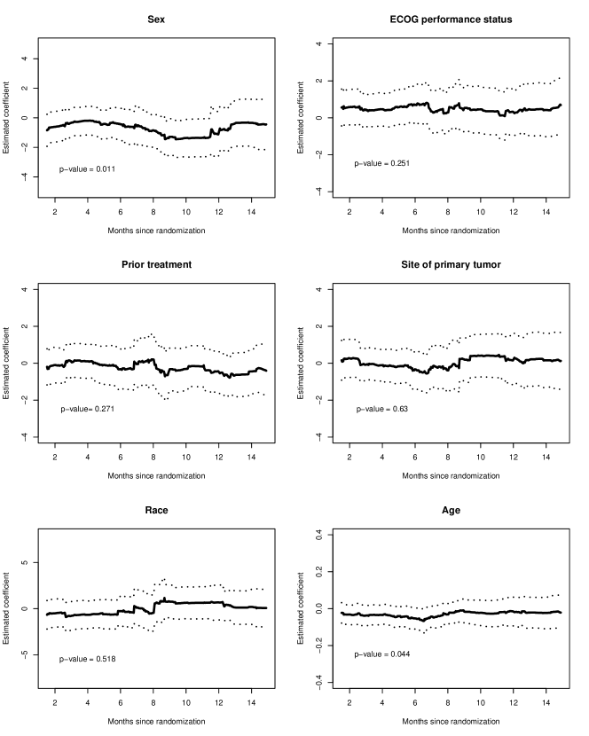
Figure 3: Plots for the estimated regression coefficients of sex, ECOG performance status, prior treatment history, site of primary tumor, race, and age, for the ”tumor response” state, along with the corresponding 95% simultaneous confidence bands and p-values based the proposed methodology.

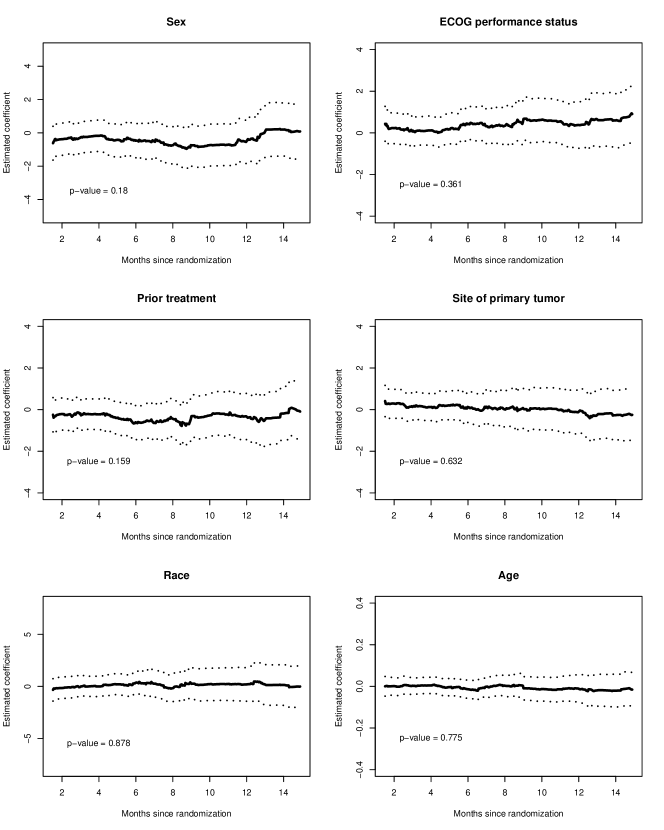
Figure 4: Plots for the estimated regression coefficients of sex, ECOG performance status, prior treatment history, site of primary tumor, race, and age, for the ”tumor response” state, along with the corresponding 95% simultaneous confidence bands and p-values based on methodology by Fine et al. (2004) for independent observations.

References

- Aalen and Johansen (1978) Aalen, O. O. and S. Johansen (1978). An empirical transition matrix for non-homogeneous markov chains based on censored observations. Scandinavian Journal of Statistics, 141–150.
- Andersen and Klein (2007) Andersen, P. K. and J. P. Klein (2007). Regression analysis for multistate models based on a pseudo-value approach, with applications to bone marrow transplantation studies. Scandinavian Journal of Statistics 34(1), 3–16.
- Andersen and Perme (2008) Andersen, P. K. and M. P. Perme (2008). Inference for outcome probabilities in multi-state models. Lifetime Data Analysis 14(4), 405.
- Azarang et al. (2017) Azarang, L., T. Scheike, and J. de Uña-Álvarez (2017). Direct modeling of regression effects for transition probabilities in the progressive illness–death model. Statistics in Medicine 36(12), 1964–1976.
- Bakoyannis (2020) Bakoyannis, G. (2020). Nonparametric tests for transition probabilities in nonhomogeneous markov processes. Journal of Nonparametric Statistics 32(1), 131–156.
- Bakoyannis (2021) Bakoyannis, G. (2021). Nonparametric analysis of nonhomogeneous multistate processes with clustered observations. Biometrics 77(2), 533–546.
- Bakoyannis and Bandyopadhyay (2022) Bakoyannis, G. and D. Bandyopadhyay (2022). Nonparametric tests for multistate processes with clustered data. Annals of the Institute of Statistical Mathematics 74(5), 837–867.
- Begg and Larson (1982) Begg, C. B. and M. Larson (1982). A study of the use of the probability-of-being-in-response function as a summary of tumor response data. Biometrics, 59–66.
- Bluhmki et al. (2018) Bluhmki, T., C. Schmoor, D. Dobler, M. Pauly, J. Finke, M. Schumacher, and J. Beyersmann (2018). A wild bootstrap approach for the aalen–johansen estimator. Biometrics 74(3), 977–985.
- Cai et al. (2000) Cai, T., L. Wei, and M. Wilcox (2000). Semiparametric regression analysis for clustered failure time data. Biometrika 87(4), 867–878.
- Chen et al. (2012) Chen, B., Y. Y. Grace, R. J. Cook, and X.-H. Zhou (2012). Marginal methods for clustered longitudinal binary data with incomplete covariates. Journal of Statistical Planning and Inference 142(10), 2819–2831.
- Cong et al. (2007) Cong, X. J., G. Yin, and Y. Shen (2007). Marginal analysis of correlated failure time data with informative cluster sizes. Biometrics 63(3), 663–672.
- Datta and Satten (2001) Datta, S. and G. A. Satten (2001). Validity of the aalen–johansen estimators of stage occupation probabilities and nelson–aalen estimators of integrated transition hazards for non-markov models. Statistics & Probability Letters 55(4), 403–411.
- Eisenhauer et al. (2009) Eisenhauer, E. A., P. Therasse, J. Bogaerts, L. H. Schwartz, D. Sargent, R. Ford, J. Dancey, S. Arbuck, S. Gwyther, M. Mooney, et al. (2009). New response evaluation criteria in solid tumours: revised recist guideline (version 1.1). European Journal of Cancer 45(2), 228–247.
- Ellis et al. (2008) Ellis, S., K. J. Carroll, and K. Pemberton (2008). Analysis of duration of response in oncology trials. Contemporary Clinical Trials 29(4), 456–465.
- Fine et al. (2004) Fine, J., J. Yan, and M. Kosorok (2004). Temporal process regression. Biometrika 91(3), 683–703.
- Forsythe (1987) Forsythe, A. B. (1987). Validity and power of tests when groups have been balanced for prognostic factors. Computational Statistics & Data Analysis 5(3), 193–200.
- Hougaard (1986) Hougaard, P. (1986). A class of multivanate failure time distributions. Biometrika 73(3), 671–678.
- Kahan and Morris (2012a) Kahan, B. C. and T. P. Morris (2012a). Improper analysis of trials randomised using stratified blocks or minimisation. Statistics in Medicine 31(4), 328–340.
- Kahan and Morris (2012b) Kahan, B. C. and T. P. Morris (2012b). Reporting and analysis of trials using stratified randomisation in leading medical journals: review and reanalysis. BMJ 345.
- Kaufman et al. (2017) Kaufman, H. L., R. H. Andtbacka, F. A. Collichio, M. Wolf, Z. Zhao, M. Shilkrut, I. Puzanov, and M. Ross (2017). Durable response rate as an endpoint in cancer immunotherapy: insights from oncolytic virus clinical trials. Journal for Immunotherapy of Cancer 5(1), 1–9.
- Kosorok (2008) Kosorok, M. R. (2008). Introduction to empirical processes and semiparametric inference. New York: Springer.
- Liu et al. (2011) Liu, D., J. D. Kalbfleisch, and D. E. Schaubel (2011). A positive stable frailty model for clustered failure time data with covariate-dependent frailty. Biometrics 67(1), 8–17.
- Pavlou et al. (2013) Pavlou, M., S. R. Seaman, and A. J. Copas (2013). An examination of a method for marginal inference when the cluster size is informative. Statistica Sinica 23(2), 791–808.
- Pocock et al. (2002) Pocock, S. J., S. E. Assmann, L. E. Enos, and L. E. Kasten (2002). Subgroup analysis, covariate adjustment and baseline comparisons in clinical trial reporting: current practiceand problems. Statistics in Medicine 21(19), 2917–2930.
- Putter et al. (2007) Putter, H., M. Fiocco, and R. B. Geskus (2007). Tutorial in biostatistics: competing risks and multi-state models. Statistics in Medicine 26(11), 2389–2430.
- Seaman et al. (2014) Seaman, S. R., M. Pavlou, and A. J. Copas (2014). Methods for observed-cluster inference when cluster size is informative: a review and clarifications. Biometrics 70(2), 449–456.
- Spiekerman and Lin (1998) Spiekerman, C. F. and D. Lin (1998). Marginal regression models for multivariate failure time data. Journal of the American Statistical Association 93(443), 1164–1175.
- Temkin (1978) Temkin, N. R. (1978). An analysis for transient states with application to tumor shrinkage. Biometrics, 571–580.
- Therasse et al. (2000) Therasse, P., S. G. Arbuck, E. A. Eisenhauer, J. Wanders, R. S. Kaplan, L. Rubinstein, J. Verweij, M. Van Glabbeke, A. T. van Oosterom, M. C. Christian, et al. (2000). New guidelines to evaluate the response to treatment in solid tumors. Journal of the National Cancer Institute 92(3), 205–216.
- van der Vaart and Wellner (1996) van der Vaart, A. W. and J. A. Wellner (1996). Weak Convergence and Empirical Processes with Applications to Statistics. New York: Springer.
- Vermorken et al. (2013) Vermorken, J. B., J. Stöhlmacher-Williams, I. Davidenko, L. Licitra, E. Winquist, C. Villanueva, P. Foa, S. Rottey, K. Skladowski, M. Tahara, et al. (2013). Cisplatin and fluorouracil with or without panitumumab in patients with recurrent or metastatic squamous-cell carcinoma of the head and neck (spectrum): an open-label phase 3 randomised trial. The Lancet Oncology 14(8), 697–710.
- Wang and Louis (2003) Wang, Z. and T. A. Louis (2003). Matching conditional and marginal shapes in binary random intercept models using a bridge distribution function. Biometrika 90(4), 765–775.
- White and Thompson (2005) White, I. R. and S. G. Thompson (2005). Adjusting for partially missing baseline measurements in randomized trials. Statistics in Medicine 24(7), 993–1007.
- Williamson et al. (2008) Williamson, J. M., H.-Y. Kim, A. Manatunga, and D. G. Addiss (2008). Modeling survival data with informative cluster size. Statistics in Medicine 27(4), 543–555.
- Zhang et al. (2011) Zhang, H., D. E. Schaubel, and J. D. Kalbfleisch (2011). Proportional hazards regression for the analysis of clustered survival data from case–cohort studies. Biometrics 67(1), 18–28.
- Zhang et al. (2008) Zhang, M., A. A. Tsiatis, and M. Davidian (2008). Improving efficiency of inferences in randomized clinical trials using auxiliary covariates. Biometrics 64(3), 707–715.
- Zhou et al. (2012) Zhou, B., J. Fine, A. Latouche, and M. Labopin (2012). Competing risks regression for clustered data. Biostatistics 13(3), 371–383.
- Zhou et al. (2022) Zhou, W., G. Bakoyannis, Y. Zhang, and C. T. Yiannoutsos (2022, 04). Semiparametric marginal regression for clustered competing risks data with missing cause of failure. Biostatistics. kxac012.