Estimation for the Cox Model with Biased Sampling Data via Risk Set Sampling

Abstract

Prevalent cohort sampling is commonly used to study the natural history of a disease when the disease is rare or it usually takes a long time to observe the failure event. It is known, however, that the collected sample in this situation is not representative of the target population which in turn leads to biased sample risk sets. In addition, when survival times are subject to censoring, the censoring mechanism is informative. In this paper, I propose a pseudo-partial likelihood estimation method for estimating parameters in the Cox proportional hazards model with right-censored and biased sampling data by adjusting sample risk sets. I study the asymptotic properties of the resulting estimator and conduct a simulation study to illustrate its finite sample performance of the proposed method. I also use the proposed method to analyze a set of HIV/AIDS data.

Keywords
Biased Sampling; Cox Regression Model, Right-censoring; Risk Set Sampling.

1 Introduction

Incident and prevalent cohort sampling designs are commonly used to study the natural history of diseases. An incident cohort sampling design is the gold standard in survival analysis. But, it can be infeasible in practice when the disease under study is rare or it usually takes a long time to observe the failure event.
A prevalent cohort sampling design is a viable alternative that follows forward subjects who have experienced an initiating event before the recruitment. The design, however, poses two challenges. Firstly, when the collected sample are subject to censoring, the censoring mechanism is informative (Asgharian and Wolfson,, 2005). Secondly, the collected sample are not a representative of the target population since a patient has to survive until the recruitment time to have a chance to be included in the study. Therefore, the collected sample is biased toward long survival times. and as such sampling is biased. Under this situation, sample risk sets do not form a random sample from the risk population and the standard methods for estimating parameters become inappropriate.
Under biased sampling design, the observed survival times are said to be left-truncated. When the incidence rate of the onset of the disease remains almost constant over time (the stationarity assumption), the type of bias is known as length-bias. The stationarity assumption is closely tied to uniform truncation distribution (Asgharian,, 2003). In fact, under some mild conditions, the stationarity assumption holds if and only if the truncation time is uniformly distributed (Asgharian et al.,, 2006).
There has been a rising interest in nonparametric and semiparametric estimation for prevalent cohort data over the last two decades. Heuchenne et al., (2020) summarized nonparametric estimation methods of the survival function when the distribution of truncation times is either partially or completely known. They developed two methods of estimating for both the truncation and the survival distributions under a semiparametric truncation model in which the truncation variable is assumed to have a certain parametric distribution. Shen et al., (2017) also provided a thorough review of the nonparametric and semiparametric estimation methods for right-censored length-biased data. In particular, the estimation methods for the Cox proportional hazards (PH) model with right-censored length-biased data can be classified into the weighted estimating equation and likelihood-based approaches. The former uses some weight functions to adjust length-biased data (Qin and Shen,, 2010). The latter, on the other hand, uses the conditional likelihood of observed survival data given the truncation times (Huang and Qin,, 2012). With right-censored and left-truncated data, Wang et al., (1993) proposed the partial likelihood method for estimation under the Cox PH model. The partial likelihood function is similar to the that of classical survival data, except for the structure of the risk set. The authors showed that the maximum partial likelihood estimator is asymptotically as efficient as an estimator obtained from the truncation likelihood function when the truncation distribution is unknown. However, when the truncation distribution is known, the partial likelihood may lead to a loss of efficiency. Wang, (1996) proposed a pseudo-partial likelihood method for estimating parameters in the Cox PH model for length-biased data in the absence of right-censoring by correcting the bias of sample risk sets. Tsai, (2009) developed a pseudo-partial likelihood method for the Cox PH model with biased sampling data by embedding the data into left-truncated data which in turn yields a more efficient estimator.
In this article, following the idea of risk set sampling (Wang,, 1996), I propose a pseudo-partial likelihood method under the Cox PH model with right-censored and biased sampling data by correcting the bias of sample risk sets. I study the large sample properties of the resulting estimator, conduct a simulation study to confirm its finite sample performance, and apply the method to analyze a dataset from the HIV-infection and AIDS.
The rest of this article is organized as follows. In Section 2, some notation, the model, and the likelihood function of the observed data are introduced. In Section 3, I first introduce the pseudo-partial likelihood method and then discuss the large sample properties of the resulting estimator. In Section 4, I conduct a simulation study to confirm the finite sample performance of the proposed method. I also apply the proposed method to analyze a a set of HIV/AIDS data. Section 5 provides some discussion and closing remarks. The Appendix includes proofs and other details.

2 Notation and Preliminaries

Let $\tilde{T}$ and $\tilde{A}$ be the survival time and the truncation time, respectively and $\tilde{\textbf{Z}}$ be the corresponding $p\times 1$ vector of covariates in a target population. Let $f_{U}(t|\textbf{z})$ and $S_{U}(t|\textbf{z})$ be the conditional probability density function and the survival function of $\tilde{T}$ given $\tilde{\textbf{Z}}=\textbf{z}$, respectively. Let further $g_{\theta}(a)$ and $G_{\theta}(a)$ be the probability density function and the distribution function of $\tilde{A}$ with a known parameter $\theta$, respectively.
Under prevalent cohort sampling, the collected sample are not representative of the target population. I therefore use different variables to distinguish them from their counterparts in the target population. Let $T$ represent the survival time, $A$ be the observed truncation time which is also called the backward recurrence time, and Z be the covariate vector in a prevalent cohort sample. Let $V$ be the time from the recruitment until failure, also known as the forward recurrence time; i.e. $V=T-A$ (see Figure 1).
Survival times in a prevalent cohort may be subject to right censoring. Let $C$ represent the time from the recruitment to censoring, called the residual censoring time. The total censoring time is therefore $\tilde{C}=A+C$. Let further $Y=\min(T,\tilde{C})$ and $\Delta=I({T\leq{\tilde{C}}})$ denote the observed survival time and the censoring indicator. The observed data $(a_{i},y_{i},\delta_{i},\textbf{z}_{i})$ for $i=1,2,\cdots,n$. are then assumed to be independent and identically distributed realizations of $(A,Y,\Delta,\textbf{Z})$.

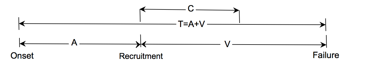
Figure 1: Positions of variables in a prevalent cohort study.

Suppose that the hazard of failure times in the target population follows the Cox PH model.

$$h({t|\tilde{\textbf{Z}}={\textbf{z}}})={h}(t)\exp({\boldsymbol{\beta}^{\prime}}{\textbf{z}}),$$ (2.1)

where $h(t)$ is an unspecified baseline hazard function and $\boldsymbol{\beta}$ is a $p\times 1$ vector of parameters.
Under prevalent cohort design, the joint distribution of $(A,T,\textbf{Z})$ is the same as that of $(\tilde{A},\tilde{T},\tilde{\textbf{Z}})$ given $\tilde{T}\geq\tilde{A}$. Then it is not hard to show that the probability density function of $(A,T)$ given ${\textbf{Z}}={\textbf{z}}$ is given by

$${f_{(A,T)}}\left({a,t\left|{\textbf{z}}\right.}\right)=\begin{cases}\frac{g_{\theta}(a){f_{U}(t\left|{\textbf{z}}\right.)}}{{\mu_{G}({\textbf{z}})}}&\mbox{ $t>a$}\\ 0&\mbox{Otherwise,}\end{cases}$$ (2.2)

where $g_{\theta}(t)$ is the probability density function of $\tilde{A}$ with some known parameter $\theta$ and

$$\mu_{G}({\textbf{z}})=E[{\tilde{T}|{\tilde{\textbf{Z}}={\textbf{z}}}}]=\int_{0}^{\infty}S_{U}(t|\textbf{z})g_{\theta}(t)dt.$$

It follows from the joint probability density function (2.2) and the Cox PH model (2.1) that the full likelihood function of the collected sample is proportional to

$$L_{F} \propto{\prod\limits_{i=1}^{n}{\left\{{\frac{{{f_{U}}({y_{i}}|{{\textbf{z}}_{i}})g_{\theta}({a_{i}})}}{{{\mu_{G}}({{\textbf{z}}_{i}})}}}\right\}}^{{\delta_{i}}}}{\left\{{\frac{{{S_{U}}({y_{i}}|{{\textbf{z}}_{i}})g_{\theta}({a_{i}})}}{{{\mu_{G}}({{\textbf{z}}_{i}})}}}\right\}^{1-{\delta_{i}}}}$$

$$=\prod\limits_{i=1}^{n}{{{\left\{{{h}({y_{i}}){\exp({{{\boldsymbol{\beta}^{\prime}}}{{\textbf{z}}_{i}}})}}\right\}}^{{\delta_{i}}}}\frac{{\exp\left\{{-{H({y_{i}}){\exp({{{\boldsymbol{\beta}^{\prime}}}{{\textbf{z}}_{i}}})}}}\right\}}}{{\mu_{G}({{\textbf{z}}_{i}})}}}g_{\theta}({a_{i}}),$$ (2.3)

where $H(.)$ is the cumulative baseline hazard function.
Although direct maximization of equation (2) with respect to $(\boldsymbol{\beta},H(.))$ yiels most efficient estimators of the parameters, it is numerically intractable especially for large sample sizes since it involves the integral of the nonparametric $H(.)$ in a complicated way. I therefore propose a pseudo-partial likelihood method by correcting the bias of sample risk sets.

3 Estimation and Asymptotic

Under classical survival data, the inference based on the partial likelihood for the Cox PH model is driven by risk sets just prior vto the failure times. For prevalent cohort data, by contrast, a subject in the target population may experience the failure event before the start of the study and hence sample risk sets do not form a random sample from the population risk sets and they require some adjustment.

3.1 Pseudo-partial Likelihood Method

Let $m$ be the number of subjects that are observed to fail at times ${t_{(1)}}<...<{t_{(m)}}$ ($m\leq n$) and ${\mathcal{R}}_{i}=\{j:{y_{j}}\geq{t_{(i)}},{\delta_{j}}=1\}$ for $i=1,...,m$, be the sample risk set of uncensored subjects. For subject $j$ in $\mathcal{R}_{i}$, define the indicator variable ${\xi_{j}}(u)$ that assumes 1 with probability ${\Omega_{C}}({u})/{\Omega_{C}}({y_{j}})$ and 0 with probability $1-{\Omega_{C}}({u})/{\Omega_{C}}({y_{j}})$ for $0<u\leq y_{j}$ where ${\Omega_{C}}(y)=\int_{0}^{y}{{S_{C}}(t)}g_{\theta}(t)dt$. The bias-adjusted risk set is then defined by

$$\tilde{\mathcal{R}}_{i}=\{j:{y_{j}}\geq{t_{(i)}},{\delta_{j}}=1,{\xi_{j}}({t_{(i)}})=1\}.$$ (3.1)

It can be shown that the subjects in $\tilde{\mathcal{R}}_{i}$ have the population risk structure. To this end, first note that given that $C$ is independent of $(A,T)$ and the distribution of $C$ does not depend on covariates, by the joint probability density function (2.2), the conditional probability of observing uncensored data given $\textbf{Z}=\textbf{z}$ is

$$P(Y=y,\delta=1|{\textbf{z}})=\int_{0}^{y}{P(T=y,A=a|{\textbf{z}})P(C\geq y-a)da}=\frac{{{f_{U}}(y|\textbf{z})}}{\mu_{G}(\textbf{z})}{\Omega_{C}}(y).$$ (3.2)

It follows from the indicator function and equation (3.2) that for subjects in $\tilde{\mathcal{R}}_{i}$, sampling $\tilde{\mathcal{R}}_{i}$ is equivalent to the sampling conditional probability of $\tilde{T}$ for $\tilde{T}\geq t_{(i)}$ because

$$pr({y_{j}}\left|{{\xi_{j}}({t_{(i)}})=1,{Y_{j}}}\right.\geq{t_{(i)}},{\delta_{j}}=1,{\textbf{z}_{j}})$$

$$=\frac{{{pr}({\xi_{j}}({t_{(i)}})=1\left|{{y_{j}},{Y_{j}}}\right.\geq{t_{(i)}},{\delta_{j}}=1,{\textbf{z}_{j}})pr({Y_{j}=y_{j}},{\delta_{j}}=1\left|{{Y_{j}}\geq{t_{(i)}},{\textbf{z}_{j}}}\right.)}}{{\int_{0}^{\infty}{{pr}({\xi_{j}}({t_{(i)}})=1\left|{y,{Y_{j}}}\right.\geq{t_{(i)}},{\delta_{j}}=1,{\textbf{z}_{j}})pr(Y_{j}=y,{\delta_{j}}=1\left|{Y_{j}\geq{t_{(i)}},{\textbf{z}_{j}}}\right.)dy}}}$$

$$=\frac{{{\{{\Omega_{C}}({t_{(i)}})/{\Omega_{C}}({y_{j}})\}}{\Omega_{C}}({y_{j}}){f_{U}}({y_{j}}\left|{{\textbf{z}_{j}}}\right.)I({y_{j}}\geq{t_{(i)}})/\mu({\textbf{z}}_{j})}}{{\int_{0}^{\infty}{{\{{\Omega_{C}}({t_{(i)}})/{\omega_{C}}(y)\}}{\Omega_{C}}(y){f_{U}}(y\left|{{\textbf{z}_{j}}}\right.)I(y\geq{t_{(i)}})/\mu({\textbf{z}}_{j})dy}}}$$

$$=\frac{{{f_{U}}({y_{j}}\left|{{\textbf{z}_{j}}}\right.)I({y_{j}}\geq{t_{(i)}})}}{{\int_{0}^{\infty}{{f_{U}}(y\left|{{\textbf{z}_{j}}}\right.)I(y\geq{t_{(i)}})dy}}}=pr({y_{j}}\left|{\tilde{T}\geq{t_{(i)}}},\right.{\textbf{z}_{j}}).$$ (3.3)

This implies that

$$pr({\textrm{subject (j) fails at}}\ t_{(i)}|{\tilde{\mathcal{R}}_{i}})\approx\frac{{{h_{(j)}}(t_{(i)}|{\textbf{z}}_{(j)})}}{{\sum\limits_{j\in{\tilde{\mathcal{R}}_{i}}}{{h_{j}}(t_{(i)}|{\textbf{z}}_{j})}}}=\frac{{\exp({{\boldsymbol{\beta}^{\prime}}}{{\textbf{z}}_{(j)}})}}{{\sum\limits_{j\in{{\tilde{\mathcal{R}}}_{i}}}{\exp({{\boldsymbol{\beta}^{\prime}}}{{\textbf{z}}_{j}})}}}$$ (3.4)

Therefore a pseudo-partial likelihood function is given by

$$L(\boldsymbol{\beta})=\prod\limits_{i=1}^{m}{\frac{{\exp({\boldsymbol{\beta}^{\prime}}{\textbf{z}_{(i)}})}}{{\sum\limits_{j\in{\tilde{\mathcal{R}}_{i}}}{\exp({\boldsymbol{\beta}^{\prime}}{\textbf{z}_{j}})}}}}.$$ (3.5)

The maximum pseudo-partial likelihood estimator is obtained by maximizing the likelihood function after inserting $\hat{\Omega}_{C}(t)$ from the Kaplan-Meier estimate of $S_{C}(t)$. Note that the (normalized) pseudo-partial score function becomes

$$U_{n}(\boldsymbol{\beta})=\frac{1}{n}\sum\limits_{i=1}^{n}{U_{i}}=\frac{1}{n}\sum\limits_{i=1}^{n}{\delta_{i}}\left[{{\textbf{z}_{i}}-\frac{{\sum\limits_{j\in{\tilde{\mathcal{R}}_{i}}}{{\textbf{z}_{j}}\exp({\boldsymbol{\beta}^{\prime}}{\textbf{z}_{j}})}}}{{\sum\limits_{j\in{\tilde{\mathcal{R}}_{i}}}{\exp({\boldsymbol{\beta}^{\prime}}{\textbf{z}_{j}})}}}}\right].$$ (3.6)

Remark 3.1.

It is not hard to show that $V_{n}(\boldsymbol{\beta})$ below is an extension of the weighted estimating function (Qin and Shen,, 2010) for length-biased sampling data to biased sampling data.

$$V_{n}(\boldsymbol{\beta})=\frac{1}{n}\sum\limits_{i=1}^{n}V_{i}=\sum\limits_{i=1}^{n}{{\delta_{i}}\left[{{\textbf{z}_{i}}-\frac{{\sum\limits_{j=1}^{n}{I({y_{j}}\geq{y_{i}}){\delta_{j}}{\textbf{z}_{j}}\exp({\boldsymbol{\beta}^{\prime}}{\textbf{z}_{j}}){{\{{\Omega_{C}}({y_{j}})\}}^{-1}}}}}{{\sum\limits_{j=1}^{n}{I({y_{j}}\geq{y_{i}}){\delta_{j}}\exp({\boldsymbol{\beta}^{\prime}}{\textbf{z}_{j}}){{\{{\Omega_{C}}({y_{j}})\}}^{-1}}}}}}\right]}$$ (3.7)

Because $E\left[{B_{li}}(y)|y_{i}\right]=\left[\Omega_{C}(y)/\Omega_{C}(y_{i})\right]{\zeta_{i}}(y)$, the difference between $V_{i}$ and $U_{i}$ is the replacement of $\xi_{j}(Y_{i})$ in $U_{i}$ by the expected value of $\xi_{j}(Y_{i})$ for given $(Y_{i},Y_{j})$. I show in the Appendix that $n^{1/2}U_{n}(\boldsymbol{\beta})$ and $n^{1/2}V_{n}(\boldsymbol{\beta})$ are asymptotically equivalent.

Remark 3.2.

The pseudo-partial likelihood function (3.5) is based on the unbiased risk sets $\tilde{\mathcal{R}}_{i}$ which, conditional on ${\mathcal{R}}_{i}$, is a random subset of ${\mathcal{R}}_{i}$ and ranges from 1 to $|{\mathcal{R}}_{i}|$. When $|\tilde{\mathcal{R}}_{i}|=1$, i.e., $\tilde{\mathcal{R}}_{i}=\{i\}$, the pseudo-partial score function (3.6) makes no contribution to the estimation of $\boldsymbol{\beta}$. As suggested by Wang, (1996), the statistical variation from the risk set sampling can be reduced by replicating the method and estimating $\boldsymbol{\beta}$ by the average of the resulting estimators. As the author pointed out, while the replication procedure does not increase the asymptotic efficiency for estimating $\boldsymbol{\beta}$, it can improve estimation when sample size is small or moderate.
Let $l$ be the repetition number and $\xi_{lj}(y_{i})$ be the indicators from the $l$th repetition for $l=1,...,L$. Let $\hat{\boldsymbol{\beta}}_{l}$ denote the $p\times 1$ estimator obtained in the $l$th repetition, and $\bar{\beta}_{L}=L^{-1}\sum\nolimits_{l=1}^{L}\hat{\boldsymbol{\beta}}_{l}$. While the replication procedure does not increase the asymptotic efficiency for estimating $\boldsymbol{\beta}$, it is expected to improve estimation when the sample size $n$ is small or moderate.

Remark 3.3.

The Breslow’s estimator (Cox,, 1972, Discussion) for estimating cumulative baseline hazard function with right-censored survival data can be adapted to right-censored general biased sampling data.
Let $y_{(i)}$ be the $i$th distinct uncensored data and $d_{i}$ be its distance from the nearest $y_{(k)}$ on the left side. We assume that the baseline hazard function $h_{0}(y)$ is piecewise constant in $y_{(k)}<y<y_{(i)}$ and let $h_{0i}=h_{0}(y_{(i)})d_{i}$. By heuristic argument and the relationship

$$1={\sum\limits_{j:{y_{j}}\geq{y_{(i)}}}{{{\left[{{h_{0i}}{\left\{{{\Omega_{C}}({y_{(i)}})/{\Omega_{C}}({y_{j}})}\right\}}\exp({{\boldsymbol{\beta}^{\prime}}}{\textbf{z}_{j}})}\right]}}}}$$

Substituting $\hat{\boldsymbol{\beta}}$ into the above equation, an estimate of $h_{0i}$ is

$${\hat{h}}_{0i}=\frac{1}{{\sum\limits_{j:{y_{j}}\geq{y_{(i)}}}{{{\left[{\{{\Omega_{C}}({y_{(i)}})/{\Omega_{C}}({y_{j}})\}\exp({\hat{\boldsymbol{\beta}^{\prime}}}{\textbf{z}_{j}})}\right]}}}}}$$

Then an estimator for the cumulative baseline hazard function becomes

$$\widehat{H_{0}}(t)=\sum\limits_{i:y_{(i)}<t}{{\hat{h}_{0i}}}$$

3.2 Asymptotic Properties

Let $N_{i}(t)=I(y_{i}\leq t,\delta_{i}=1)$ represent the counting process of observed failure times. For each $(l,y)$ define

$${B_{lj}}(y)=\begin{cases}{\xi_{lj}(y)}&\mbox{if}\ {y_{j}}\geq y\ \mbox{and}\ \delta_{j}=1,\\ 0&\mbox{Otherwise}\end{cases}$$ (3.8)

Note that $E\left[{B_{li}}(y)|Y_{i}\right]=\left[\Omega_{C}(y)/\Omega_{C}(Y_{i})\right]{\zeta_{i}}(y)$ where ${\zeta_{i}}(y)=I({y_{i}}\geq y,{\delta_{i}}=1)$ is the at-risk function for uncensored observations. Define ${S_{lB}^{(k)}}({\boldsymbol{\beta}},y)=n^{-1}\sum\nolimits_{j=1}^{n}{B_{lj}(y){\textbf{z}}_{j}^{\otimes k}\exp({\boldsymbol{\beta}^{\prime}}}{\textbf{z}_{j}})$ for $k=0,1,2$, with expectations ${s^{(k)}}({\boldsymbol{\beta}},y)$ where for a column vector a, ${\textbf{a}}^{\otimes 2}={\textbf{a}}{\textbf{a}^{\prime}}$, ${\textbf{a}}^{\otimes 1}={\textbf{a}}$, and ${\textbf{a}}^{\otimes 0}=1$. Then the pseudo-partial score function (3.6) can be expressed as

$$U_{n}(\boldsymbol{\beta})=\frac{1}{n}\sum\limits_{i=1}^{n}U_{li}=\frac{1}{n}\sum\limits_{i=1}^{n}{\delta_{i}}{\left[{{{\textbf{z}}_{i}}-\frac{{S_{lB}^{(1)}(\boldsymbol{\beta},{Y_{i}})}}{{S_{lB}^{(0)}(\boldsymbol{\beta},{y_{i}})}}}\right]}$$ (3.9)

For $i=1,...,n$, define stochastic process

$${M_{i}}(t)={N_{i}}(t)-\int_{0}^{t}\{{\Omega_{C}}(y)/{\Omega_{C}}({y_{i}})\}{\zeta_{i}}(y)h(y|\textbf{z}_{i})dy.$$ (3.10)

The stochastic process can be interpreted as the difference between the observed number of events and the expected number of events under the assumed model until time $t$. When model (2.1) is correctly specified, this becomes a mean zero stochastic process because

$$E\left[{{M_{i}}(t)}\right] =E\left[E[{{N_{i}}(t)}|{\textbf{Z}}_{i}]\right]-E\left[{\int_{0}^{t}{h(y\left|{{{\textbf{Z}}_{i}}}\right.){\Omega_{C}}(y)E\left[{\zeta_{i}}(y)/{\Omega_{C}}({Y_{i}})|{\textbf{Z}}_{i}\right]dy}}\right]$$

$$=E\left[{{\int_{0}^{t}{\frac{{{f_{U}}(y\left|{{{\textbf{Z}}_{i}}}\right.)}}{{\mu_{G}({{\textbf{Z}}_{i}})}}{\Omega_{C}}(y)dy}}}\right]-E\left[{\int_{0}^{t}{h(y\left|{{{\textbf{Z}}_{i}}}\right.){\Omega_{C}}(y)\frac{{{S_{U}}(y\left|{{{\textbf{Z}}_{i}}}\right.)}}{{\mu_{G}({{\textbf{Z}}_{i}})}}dy}}\right]$$

$$=0$$

Therefore when $S_{C}$ is known, $U_{n}(\boldsymbol{\beta})$ can be asymptotically represented by the following independent and identically distributed summation of the mean zero stochastic processes.

$$U_{n}(\boldsymbol{\beta})=\frac{1}{n}\sum\limits_{i=1}^{n}\int_{0}^{\tau}\left\{\textbf{z}_{i}-\frac{s^{(1)}({\boldsymbol{\beta}},v)}{s^{(0)}({\boldsymbol{\beta}},v)}\right\}dM_{i}(v)+o_{P}(n^{-1/2})$$

When $S_{C}$ is unknown, it can be replaced by its consistent Kaplan-Meier estimator $\hat{S}_{C}$. Let $\tilde{S}_{lB}^{(k)}({\boldsymbol{\beta}},v)$ be an estimate of $S_{lB}^{(k)}({\boldsymbol{\beta}},v)$ after inserting $\hat{S}_{C}$. Then

$$\tilde{U}_{n}(\boldsymbol{\beta})=\frac{1}{n}\sum\limits_{i=1}^{n}\int_{0}^{\tau}\left\{\textbf{z}_{i}-\frac{\tilde{S}_{lB}^{(1)}({\boldsymbol{\beta}},v)}{\tilde{S}_{lB}^{(0)}({\boldsymbol{\beta}},v)}\right\}dN_{i}(v)$$ (3.11)

I show in the Appendix that under the regularity conditions, $n^{1/2}\tilde{U}_{n}(\boldsymbol{\beta})$ converges weakly to a mean zero Gaussian process.
Let $\Gamma_{n}(\boldsymbol{\beta})=\partial{\tilde{U}}_{n}(\boldsymbol{\beta})/\partial{\boldsymbol{\beta}}$ and $\Sigma$ be the variance-covariance matrix of the sampling distribution of $n^{1/2}\tilde{U}_{n}(\boldsymbol{\beta})$. The following theorem presents the asymptotic properties of the maximum pseudo-partial likelihood estimator.

Theorem 3.1.

Suppose that conditions C1-C3 in the Appendix hold. For each positive integer $L$, as $n\to\infty$, $\hat{\boldsymbol{\beta}}_{L}$ converges to the true parameter ${\boldsymbol{\beta}}_{0}$ in probability. Furthermore, $n^{1/2}(\hat{\boldsymbol{\beta}}_{L}-{\boldsymbol{\beta}}_{0})$ converges weakly to a mean zero Gaussian distribution with covariance matrix $\Psi({{\boldsymbol{\beta}}_{0}})=\Gamma^{-1}{({{\boldsymbol{\beta}}_{0}})}\Sigma\Gamma^{-1}{({{\boldsymbol{\beta}}_{0}})}$ where $\Gamma(\boldsymbol{\beta})=\mathop{\lim}\limits_{n\to\infty}\Gamma_{n}(\boldsymbol{\beta})$.

The regularity conditions and the proof are provided in the Appendix.

4 Numerical Studies

4.1 Simulation Study

I conducted a simulation study to evaluate the finite sample performance of the resulting pseudo-partial likehood (PPL) estimates compared to those of the partial likelihood (PL) method (Wang et al.,, 1993). I set the recruitment time to $\nu=10$ and generated the onset times from an exponential distribution with mean 1. The covariates ${\tilde{Z}}_{1}$ and ${\tilde{Z}}_{2}$ were generated from a standard normal distribution and a Bernoulli distribution with probability $p=P({\tilde{Z}}_{1}>0)$, respectively. Then the hazards of survival times were generated from the Cox PH model as $h_{1}(t|{\tilde{Z}}_{1}=z_{1},{\tilde{Z}}_{2}=z_{2})=2\exp(0.5z_{1}+z_{2})$, $h_{2}(t|{\tilde{Z}}_{1}=z_{1},{\tilde{Z}}_{2}=z_{2})=2t\exp(0.5z_{1}+z_{2})$, and $h_{3}(t|{\tilde{Z}}_{1}=z_{1},{\tilde{Z}}_{2}=z_{2})=3t^{2}\exp(0.5z_{1}+z_{2})$ which represent constant, increasing and U-shape hazards, respectively. I considered the sample size of $n=200$ and $n=400$. The residual censoring times are generated from a uniform distribution on $(0,\theta)$ where $\theta$ yields 0%, 20% or 40% rates of censoring. I repeated this simulation $N=1000$ times and summarized the results.
Table 1 reports the simulation results from the estimation methods under the Cox PH model with right-censored biased sampling data in terms of empirical bias (Bias), empirical standard deviation (ESD), and the averaged robust standard error (ASE) of the estimates. The results suggest that the PPL estimates are almost unbiased as those of the PL method. However, the PPL estimates are more efficient than those of the PL method. This is because the PPL method takes the information in the parametric distribution of the truncation distribution into account. Also, the ESD and the ASE of the estimates from the PPL method are almost equal. These results remain the same in different scenarios including the type of hazards, the censoring rates, and sample size. It should be pointed out increasing the censoring rates resulted in an increase in the empirical bias and standard deviations of the estimates while increasing the sample size to $n=400$ has improved the results in terms of accuracy and precision. Nevertheless, the pattern of the results remained unchanged for all scenarios. It is also noteworthy that the proposed method may become unstable for large censoring rates due to unstable weight estimates. However, the method outperforms the partial likelihood method for low and moderate rates of censoring.

Table 1: Simulation results on the estimation method for the Cox PH model with biased sampling data when truncation times follow Exponential distribution; PL: partial likelihood; PPL: pseudo-partial likelihood; C: censoring rate; Bias: empirical Bias; ESD: empirical standard deviation; ASE: average standard error; $n_{1}=200$; $n_{2}=400$; $h_{1}$: constant baseline hazard; $h_{2}$: increasing baseline hazard; $h_{3}$: U-shape baseline hazard.

	C		PL		PPL
$h_{1}$		Bias ($\beta_{1}$,$\beta_{2}$)	ESD ($\beta_{1}$,$\beta_{2}$)	Bias ($\beta_{1}$,$\beta_{2}$)	ESD ($\beta_{1}$,$\beta_{2}$)	ASE ($\beta_{1}$,$\beta_{2}$)
	0%	(0.001, 0.007)	(0.084, 0.158)	(-0.003, 0.001)	(0.067, 0.144)	(0.062, 0.141)
$n_{1}$	20%	(-0.003, 0.008)	(0.093, 0.173)	(-0.005, 0.005)	(0.078, 0.165)	(0.072, 0.169)
	40%	(0.005, 0.009)	(0.106, 0.194)	(-0.008, -0.009)	(0.090, 0.187)	(0.088, 0.183)
	0%	(0.001, 0.005)	(0.059, 0.138)	(-0.001, 0.001)	(0.049, 0.122)	(0.045, 0.125)
$n_{2}$	20%	(0.002, 0.007)	(0.065, 0.157)	(-0.003, 0.003)	(0.055, 0.145)	(0.052, 0.153)
	40%	(-0.004, 0.008)	(0.074, 0.173)	(-0.006, -0.007)	(0.068, 0.160)	(0.076, 0.166)
$h_{2}$
	0%	(-0.004, 0.007)	(0.083, 0.163)	(0.002, 0.002)	(0.074, 0.153)	(0.071, 0.157)
$n_{1}$	20%	(0.007, 0.005)	(0.090, 0.178)	(0.005, 0.004)	(0.081, 0.169)	(0.085, 0.173)
	40%	(-0.008, 0.004)	(0.104, 0.203)	(-0.008, -0.007)	(0.094, 0.182)	(0.103, 0.190)
	0%	(-0.003, 0.017)	(0.075, 0.158)	(0.001, -0.002)	(0.065, 0.139)	(0.075, 0.144)
$n_{2}$	20%	(-0.005, 0.020)	(0.084, 0.165)	(0.004, 0.003)	(0.073, 0.147)	(0.081, 0.152)
	40%	(0.008, 0.021)	(0.091, 0.184)	(-0.006, -0.005)	(0.088, 0.175)	(0.094, 0.181)
$h_{3}$
	0%	(0.005, 0.003)	(0.082, 0.161)	(0.002, -0.003)	(0.078, 0.143)	(0.075, 0.147)
$n_{1}$	20%	(-0.007, 0.004)	(0.091, 0.179)	(0.004, 0.005)	(0.086, 0.154)	(0.088, 0.161)
	40%	(0.008, 0.008)	(0.105, 0.206)	(-0.005, -0.006)	(0.099, 0.193)	(0.105, 0.198)
	0%	(0.002, 0.001)	(0.057, 0.113)	(-0.001, 0.001)	(0.057, 0.102)	(0.053, 0.104)
$n_{2}$	20%	(-0.004, 0.002)	(0.063, 0.125)	(0.004, -0.002)	(0.063, 0.116)	(0.060, 0.113)
	40%	(-0.006, 0.005)	(0.073, 0.144)	(-0.007, -0.005)	(0.073, 0.128)	(0.076, 0.133)

4.2 HIV-infection and AIDS

I employ the pseudo-partial likelihood method to estimate the regression coefficients in the Cox PH model for a set of prevalent cohort data from the Amsterdam Cohort Study on HIV infection and AIDS (Geskus,, 2000). The data were collected among homosexual men who had experienced HIV-infection prior to the study recruitment, but none developed AIDS as discussed in Geskus, (2000). While for those who are prospectively identified, the midpoint of the date of the last seronegative test and the first seropositive test was considered as the date of seroconversion. For seroprevalent cases, the situation is different. Geskus, (2000) has thoroughly studied this issue and presented a marker-based approach, using CD4 counts, for imputing missing dates of seroconversion for such cases.
The data set consist of $n=204$ prevalent cases who have been infected by HIV before the recruitment time. The survival time the time from HIV-infection to AIDS, the left-truncation variable is the time between HIV-infection and study recruitment. The covariates are age at HIV infection and a dichotomous variable CCR5 (C-C motif chemokine receptor 5) genotype with levels WW (wild type allele on both chromosomes) and WM (mutant allele on one chromosome). Among 204 patients, the survival time of 57 subjects (28%) were right-censored by the end of study. The purpose is to study the impact of the covariates at HIV infection on the survival times under the assumption that their hazard follows a Cox PH model.
I have estimated the truncation distribution using the nonparametric method (the conditional MLE) of Wang, (1991). Figure 2 depicts this estimator (red curve) and indicates an exponential trend between 1.5 and 2.5 years. Following Rabhi and Asgharian, (2020), the Weibull distribution with the shape parameter value 4.80 and scale parameter value 2.04 (blue dashed) seems to support the nonparametric estimator of the truncation distribution (red line).
Table 2 reports the estimates , their standard errors of the effects of age and CCR5, and their p-values under the Cox PH model for the HIV/AIDS data using the proposed pseudo-partial (PPL) method and the partial likelihood (PL) method (Wang et al.,, 1993). Both methods suggest that there is strong evidence that the patients’ age at HIV infection and WW genotype are positively associated with the survival times at 5% significance level.

Table 2: Estimated regression coefficients and their standard errors under the Cox PH model for the HIV/AIDS data; PL: partial likelihood; PPL: pseudo-partial likelihood; Est: estimated regression coefficients; SE: standard error.

	AGE	CCR5
Methods	Est (SE)	Est (SE)	P-Value (AGE, CCR5)
PL	0.041 (0.013)	0.892 (0.233)	(0.002, 0.000)
PPL	0.022 (0.010)	0.673 (0.228)	(0.027, 0.003)

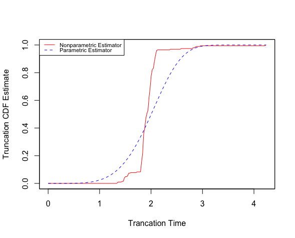
Figure 2: Nonparametric estimator (solid line) and parametric estimator based on Weibull family (dashed line).

5 Discussion

In this article, I proposed a pseudo-partial likelihood method for estimating parameters in the Cox PH model for right-censored biased sampling data via risk set sampling by correcting the bias of sample risk sets. I further studied the asymptotic properties of the resulting estimator. The simulation study showed that the resulting estimator outperform the maximum partial likelihood estimator when the truncation distribution is known. I also used the proposed method to analyze a set of HIV/AIDS data.
Although the residual censoring distribution was assumed to be independent of covariates, the methods can be adapted to account for covariate-dependent censoring. If the censoring distribution depends on covariates, then the function $\Omega_{C}(t)$ needs to be replaced by $\Omega_{C}(t|\textbf{z})=\int_{0}^{t}S_{C}(u|\textbf{z})du$, respectively. When covariates are discrete, the conditional weight functions can be consistently estimated by ${\hat{\Omega}}_{C}(t|\textbf{z})=\int_{0}^{t}{\hat{S}}_{C}(u|\textbf{z})g_{\theta}(u)du$, where ${\hat{S}}_{C}(t|\textbf{z})$ is obtained by the Kaplan-Meier estimator. For continuous covariates, we can either consider a regression model for the censoring distribution or adopt the local Kaplan-Meier estimator (Wang and Wang,, 2014). A careful investigation on these topics is warranted.

6 Appendix

We assume the following regularity conditions to establish the asymptotic properties of the estimator.

1. The covariate vector Z is a bounded random vector and ${\boldsymbol{\beta}}_{0}$ lies in a compact set $\mathcal{B}$.

2. $P(C>0)>0$.

3. $S_{U}(t)$ and $S_{C}(t)$ are absolutely continuous for $t\in[0,\tau]$ where $\tau=\sup\left\{t:P(Y\geq t)>0\right\}$.

4. $\Gamma({\boldsymbol{\beta}}_{0})$ is positive definite where $\Gamma(\boldsymbol{\beta})=\mathop{\lim}\limits_{n\to\infty}{\Gamma_{n}}(\boldsymbol{\beta})$ and $\Gamma_{n}(\boldsymbol{\beta})=-\partial U_{n}(\boldsymbol{\beta})/\partial{\boldsymbol{\beta}}$.

Proof of Theorem 3.1

To show the consistency, we consider the following log pseudo-partial likelihood function.

$$K_{n}(\boldsymbol{\beta})=\frac{1}{n}\sum\limits_{i=1}^{n}{\int_{0}^{\tau}{\left[{{{({\boldsymbol{\beta}}-{{\boldsymbol{\beta}}_{0}})^{\prime}}}{{\textbf{z}}_{i}}-\log\left\{{\frac{{S_{lB}^{(0)}({\boldsymbol{\beta}},t)}}{{S_{lB}^{(0)}({\boldsymbol{\beta}}_{0},t)}}}\right\}}\right]}}dN_{i}(t).$$

Note that $\Gamma_{n}(\boldsymbol{\beta})=\frac{\partial^{2}K_{n}(\boldsymbol{\beta})}{\partial{\boldsymbol{\beta}}\partial{\boldsymbol{\beta}}}$. Further, for any ${\boldsymbol{\beta}}\in\mathcal{B}$, as $n\to\infty$, $\Gamma_{n}(\boldsymbol{\beta})$ converges almost surely to $\Gamma$ which is assumed to be positive definite. This implies that $K_{n}({\boldsymbol{\beta}})$ is a concave function of $\boldsymbol{\beta}$. Therefore, the unique maximizer of $K_{n}({\boldsymbol{\beta}})$ converges in probability to the unique maximizer of $K({\boldsymbol{\beta}})$ (Andersen and Gill,, 1982) or $\hat{\boldsymbol{\beta}}$ converges in probability to ${\boldsymbol{\beta}}_{0}$. This completes the proof of consistency.
For the proof of asymptotic normality, we first define

$${S^{(k)}}({\boldsymbol{\beta}},y)=n^{-1}\sum\limits_{j=1}^{n}{\textbf{z}}_{j}^{\otimes k}\exp({{\boldsymbol{\beta}}^{T}}{\textbf{z}_{j}}){\{{\Omega_{C}}(y)/{\Omega_{C}}({y_{j}})\}{\zeta_{j}}(y)},\quad k=0,1,2.$$

Also, $n^{1/2}{\tilde{V}}_{n}(\boldsymbol{\beta})$ defined in (3.11) can be expanded as

$${n^{-1/2}}\sum\limits_{i=1}^{n}{\int_{0}^{\tau}{\left\{{{\textbf{z}_{i}}-\frac{{S^{(1)}(\boldsymbol{\beta},t)}}{{S^{(0)}(\boldsymbol{\beta},t)}}}\right\}dN_{i}(t)}}+{n^{-1/2}}\sum\limits_{i=1}^{n}{\int_{0}^{\tau}{\left\{{\frac{{\tilde{S}^{(1)}(\boldsymbol{\beta},t)}}{{\tilde{S}^{(0)}(\boldsymbol{\beta},t)}}-\frac{{S^{(1)}(\boldsymbol{\beta},t)}}{{S^{(0)}(\boldsymbol{\beta},t)}}}\right\}dN_{i}(t)}}.$$

From Remark 3.1, $n^{1/2}{\tilde{U}}_{n}(\boldsymbol{\beta})$ and $n^{1/2}{\tilde{V}}_{n}(\boldsymbol{\beta})$ are asymptotically equivalent (see the proof in the Appendix). Moreover,

$$n^{1/2}{\tilde{V}}_{n}(\boldsymbol{\beta})=\frac{1}{{\sqrt{n}}}\sum\limits_{i=1}^{n}{\int_{0}^{\tau}{\left\{{{\textbf{z}_{i}}-\frac{{s^{(1)}(\boldsymbol{\beta},t)}}{{s^{(1)}(\boldsymbol{\beta},t)}}}\right\}dM_{i}(t)}}+\frac{1}{{\sqrt{n}}}\sum\limits_{i=1}^{n}{\int_{0}^{\tau}{G(\boldsymbol{\beta},t)\frac{{d{M_{Ci}}(t)}}{{\pi(t)}}}}+o_{P}(1),$$ (6.1)

where, if we let $H_{C}(t)$ be the hazard function for the residual censoring, then

$${{M}_{Ci}}(t)=I({V_{i}}\leq t,{\delta_{i}}=0)-\int_{0}^{t}{I({V_{i}}\geq u)d{{H}_{C}}}(u).$$

In addition, if we define $\pi(t)=S_{C}(t)S_{V}(t)$ and further ${{h}_{k}}(t)=I(t\leq{Y_{k}})\int_{t}^{{Y_{k}}}{{{S}_{C}}}(u)du$, then we have

$$G(\boldsymbol{\beta},t)=\mathop{\lim}\limits_{n\to\infty}\frac{1}{{{n^{2}}}}\sum\limits_{i=1}^{n}{\sum\limits_{k=1}^{n}{\frac{{{\zeta_{k}}({y_{i}}){\Omega}_{C}(Y_{i}){{\textbf{Z}}_{k}}\exp({{\boldsymbol{\beta}^{\prime}}}{{\textbf{z}}_{k}})\left[{1/{{\Omega}_{C}}({y_{k}})}\right]^{2}{{h}_{k}}(t)}}{{S^{(0)}(\boldsymbol{\beta},{Y_{i}})}}}}.$$

Note that $(\hat{\Omega}_{C}(Y_{k})-\Omega_{C}(Y_{k}))$ can be expressed as sum of independent and identically distributed (i.i.d) martingale processes (Pepe and Fleming,, 1991) as below.

$${n^{1/2}}({\hat{\Omega}_{C}}({Y_{K}})-{\Omega_{C}}({Y_{K}}))={n^{-1/2}}\sum\limits_{j=1}^{n}{\int_{0}^{\tau}{{h_{k}}(t)\frac{{d{M_{Cj}}(t)}}{{\pi(t)}}}}.$$

By a similar argument to that of Qin and Shen, (2010), the terms in equation (6.1) are summation of i.i.d zero-mean martingale processes. Hence, under the regularity conditions C1-C3, by the martingale central limit theorem, $n^{1/2}{\tilde{V}}_{n}(\boldsymbol{\beta})$ converges weakly to a zero-mean Gaussian process with covariance matrix

$$\Sigma=E\left[{\int_{0}^{\tau}{{\left({{\textbf{Z}_{i}}-\frac{{s^{(1)}(\boldsymbol{\beta},t)}}{{s^{(0)}(\boldsymbol{\beta},t)}}}\right)dM_{i}(t)+\frac{{G(\boldsymbol{\beta},t)}}{{\pi(t)}}d{M_{Ci}}(t)}}}\right]^{\otimes 2}.$$

Let $\hat{\boldsymbol{\beta}}$ be a solution to ${\tilde{V}}_{n}(\boldsymbol{\beta})=\textbf{0}$. By Taylor expansion, we have

$$n^{1/2}(\hat{\boldsymbol{\beta}}-{\boldsymbol{\beta}}_{0})=\{\Gamma_{n}({\boldsymbol{\beta}}^{*})\}^{-1}n^{1/2}{\tilde{V}}_{n}(\boldsymbol{\beta})+o_{P}(1),$$

where ${\boldsymbol{\beta}}^{*}$ is on the line segment between $\hat{\boldsymbol{\beta}}$ and ${\boldsymbol{\beta}}_{0}$. Since $\hat{\boldsymbol{\beta}}$ is consistent for ${\boldsymbol{\beta}}_{0}$ and $\Gamma$ is continuous at ${\boldsymbol{\beta}}_{0}$, we see that $\Gamma_{n}(\boldsymbol{\beta})$ and as such $\Gamma_{n}({\boldsymbol{\beta}}^{*})$ converge to $\Gamma$ almost surely. Therefore, by Slutsky’s theorem, $\sqrt{n}(\hat{\boldsymbol{\beta}}-{\boldsymbol{\beta}}_{0})$ converges to a zero-mean Gaussian distribution with covariance matrix $\Psi({{\boldsymbol{\beta}}_{0}})=\Gamma^{-1}({{\boldsymbol{\beta}}_{0}})\Sigma\Gamma^{-1}({{\boldsymbol{\beta}}_{0}})$. This completes the proof.

Remark 6.1.

The Hessian matrix $\Gamma(\boldsymbol{\beta})$ and the covariance matrix $\Sigma$ can be consistently estimated by $\widehat{\Gamma}_{n}$ and $\widehat{\Sigma}$, respectively, where $\widehat{\Gamma}_{n}=\Gamma_{n}(\hat{\boldsymbol{\beta}})$ and

$$\widehat{\Sigma}={n^{-1}}\sum\limits_{i=1}^{n}{\int_{0}^{\tau}{\left\{{\left({{\textbf{z}_{i}}-\frac{{\tilde{S}^{(1)}(\hat{\boldsymbol{\beta}},t)}}{{\tilde{S}^{(0)}(\hat{\boldsymbol{\beta}},t)}}}\right)d\widehat{M}_{i}(t)+\frac{{\widehat{G}(t)}}{{\bar{y}(t)}}d{{\widehat{M}}_{Ci}}(t)}\right\}^{\otimes 2}}},$$

where ${{\widehat{M}}_{Ci}}(t)=I({y_{i}}\leq t,{\delta_{i}}=0)-\int_{0}^{t}{I({y_{i}}\geq u)d{{\widehat{H}}_{C}}}(u)$, $\bar{y}(t)={n^{-1}}\sum\limits_{i=1}^{n}{I(\min({c_{i}},{v_{i}})>t)}$,
and ${{\hat{h}}_{k}}(t)=I(t\leq{y_{k}})\int_{t}^{{y_{k}}}{{{\hat{S}}_{C}}}(u)du$. In addition, $\widehat{H}_{C}(t)$ is the Nelson-Aalan estimator for the residual censoring time, and

$$\widehat{G}(t)=\mathop{\lim}\limits_{n\to\infty}\frac{1}{{{n^{2}}}}\sum\limits_{i=1}^{n}{\sum\limits_{k=1}^{n}{\frac{{{\zeta_{i}}({y_{i}}){\hat{\Omega}}_{C}(y_{i}){{\textbf{z}}_{k}}\exp({{\hat{\boldsymbol{\beta}^{\prime}}}}{{\textbf{z}}_{k}})\left[{1/{{\hat{\Omega}}_{C}}({y_{k}})}\right]^{2}{{\hat{h}}_{k}}(t)}}{{\tilde{S}^{(0)}(\hat{\boldsymbol{\beta}},{y_{i}})}}}}$$

The covariance matrix $\Psi({{\boldsymbol{\beta}}})$ can then be consistently estimated by $\widehat{\Gamma}_{n}^{-1}{\widehat{\Sigma}}\widehat{\Gamma}_{n}^{-1}$.

Proof of Remark 3.1

Let $F^{u}(t)=P(Y\leq t,\Delta=1)$ be the distribution functions of uncensored data. The proof is carried out similar to that of Wang, (1996). Since $E\left[{B_{lj}}(t)|Y_{j}\right]=\left[\Omega(t)/\Omega_{C}(Y_{j})\right]{\zeta_{j}}(t)$, we have

$$E\left[S^{(k)}({\boldsymbol{\beta}},t)\right]=E\left\{E\left[S_{lB}^{(k)}({\boldsymbol{\beta}},t)|{\textbf{Z}}_{j},Y_{j}\right]\right\}=s^{(k)}({\boldsymbol{\beta}},t)$$

The regression coefficients in the Cox PH model can be estimated by replacing ${\xi_{j}}(Y_{i})$ in $U_{n}({\boldsymbol{\beta}})$ with their expected value given $(Y_{i},Y_{j})$ which yields the below weighted estimating function.

$${V_{n}(\boldsymbol{\beta})}=\frac{1}{n}\sum\limits_{i=1}^{n}{V_{i}}(\boldsymbol{\beta})=\frac{1}{n}\sum\limits_{i=1}^{n}{\delta_{i}\left[{{\textbf{z}_{i}}-\frac{{S^{(1)}}({\boldsymbol{\beta}},y_{i})}{{S^{(0)}}({\boldsymbol{\beta}},y_{i})}}\right]}.$$ (6.2)

To show the asymptotic equivalency, I expand ${n^{1/2}}U_{n}(\boldsymbol{\beta})$ as

$${n^{-1/2}}\sum\limits_{i=1}^{n}{{\delta_{i}}\left[{{{\textbf{z}}_{i}}-\frac{{{s^{(1)}}(\boldsymbol{\beta},{y_{i}})}}{{{s^{(0)}}(\boldsymbol{\beta},{y_{i}})}}}\right]}-{n^{-1/2}}\int_{0}^{\tau}{\left[{\frac{{S_{lB}^{(1)}(\boldsymbol{\beta},{t})}}{{S_{lB}^{(0)}(\boldsymbol{\beta},{t})}}-\frac{{{s^{(1)}}(\boldsymbol{\beta},t)}}{{{s^{(0)}}(\boldsymbol{\beta},t)}}}\right]}d\hat{F}^{u}(t),$$ (6.3)

where $\hat{F}^{u}$ is the empirical distribution function of $F^{u}$. Applying Taylor expansion, we obtain

$${n^{1/2}}S_{lB}^{(1)}(\boldsymbol{\beta},t)\left[{S_{lB}^{(0)}(\boldsymbol{\beta},t)-{s^{(0)}}(\boldsymbol{\beta},t)}\right]={n^{1/2}}{s^{(1)}}(\boldsymbol{\beta},t)\left[{S_{lB}^{(0)}(\boldsymbol{\beta},t)-{s^{(0)}}(\boldsymbol{\beta},t)}\right]+{o_{P}}(1).$$

The second term in (6.3) can be further expressed as

$$-{n^{-1/2}}\sum\limits_{i=1}^{n}{\int_{0}^{\tau}{\frac{{{B_{li}}(t)\exp({{{\boldsymbol{\beta}^{\prime}}}{{\textbf{z}}_{i}}})}}{{{s^{(0)}}(\boldsymbol{\beta},t)}}}}\left[{{{\textbf{z}}_{i}}-\frac{{{s^{(1)}}(\boldsymbol{\beta},t)}}{{{s^{(0)}}(\boldsymbol{\beta},t)}}}\right]d\hat{F}^{u}(t)+{o_{P}}(1).$$

Similarly, ${n^{1/2}}{V_{n}(\boldsymbol{\beta})}$ can be expanded as

$${n^{-1/2}}\sum\limits_{i=1}^{n}{{\delta_{i}}\left[{{{\textbf{z}}_{i}}-\frac{{{s^{(1)}}(\boldsymbol{\beta},{y_{i}})}}{{{s^{(0)}}(\boldsymbol{\beta},{y_{i}})}}}\right]}-{n^{-1/2}}\int_{0}^{\tau}{\left[{\frac{{S^{(1)}(\boldsymbol{\beta},{t})}}{{S^{(0)}(\boldsymbol{\beta},{t})}}-\frac{{{s^{(1)}}(\boldsymbol{\beta},t)}}{{{s^{(0)}}(\boldsymbol{\beta},t)}}}\right]}d\hat{F}^{u}(t).$$ (6.4)

The second term in (6.4) is asymptotically equivalent to

$$-{n^{-1/2}}\sum\limits_{i=1}^{n}{\int_{0}^{\tau}{\frac{{\left\{{{\Omega_{C}}(t)/{\Omega_{C}}({y_{i}})}\right\}{\zeta_{i}}(t)\exp({{\boldsymbol{\beta}^{\prime}}{{\textbf{z}}_{i}}})}}{{{s^{(0)}}(\boldsymbol{\beta},t)}}}}\left[{{{\textbf{z}}_{i}}-\frac{{{s^{(1)}}(\boldsymbol{\beta},t)}}{{{s^{(0)}}(\boldsymbol{\beta},t)}}}\right]d\hat{F}^{u}(t)+{o_{P}}(1).$$

Thus, the difference of the two estimating functions can be expressed as

$${n^{-1}}\sum\limits_{i=1}^{n}{{U_{li}}}(\boldsymbol{\beta})-{n^{-1}}\sum\limits_{i=1}^{n}{V_{i}}(\boldsymbol{\beta})$$

$$={n^{-1}}\int_{0}^{\tau}{\left\{{\frac{{{S^{(1)}}({\boldsymbol{\beta}},t)}}{{{S^{(0)}}({\boldsymbol{\beta}},t)}}-\frac{{{s^{(1)}}({\boldsymbol{\beta}},t)}}{{{s^{(0)}}({\boldsymbol{\beta}},t)}}}\right\}d\hat{F}^{u}(t)}-{n^{-1}}\int_{0}^{\tau}{\left\{{\frac{{S_{lB}^{(1)}({\boldsymbol{\beta}},t)}}{{S_{lB}^{(0)}({\boldsymbol{\beta}},t)}}-\frac{{{s^{(1)}}({\boldsymbol{\beta}},t)}}{{{s^{(0)}}({\boldsymbol{\beta}},t)}}}\right\}d\hat{F}^{u}(t)}$$

$$={n^{-1}}\sum\limits_{i=1}^{n}{\int_{0}^{\tau}{\frac{{\left[{\left\{{{\Omega_{C}}(t)/{\Omega_{C}}({y_{i}})}\right\}{\zeta_{i}}(t)-{B_{li}}(t)}\right]\exp({\boldsymbol{\beta}^{\prime}}{{\textbf{z}}_{i}})}}{{{s^{(0)}}({\boldsymbol{\beta}},t)}}}}\left\{{{{\textbf{z}}_{i}}-\frac{{{s^{(1)}}({\boldsymbol{\beta}},t)}}{{{s^{(0)}}({\boldsymbol{\beta}},t)}}}\right\}d\hat{F}^{u}(t)+{o_{P}}(1)$$

$$={n^{-2}}\sum\limits_{i=1}^{n}{\sum\limits_{j=1}^{n}\frac{{\left[{\left\{{{\Omega_{C}}({y_{j}})/{\Omega_{C}}({y_{i}})}\right\}{\zeta_{i}}({y_{j}})-{B_{li}}({y_{j}})}\right]\exp({{\boldsymbol{\beta}^{\prime}}{{\textbf{z}}_{i}}})}}{{{s^{(0)}}(\boldsymbol{\beta},{y_{j}})}}\left[{{{\textbf{z}}_{i}}-\frac{{{s^{(1)}}(\boldsymbol{\beta},{y_{j}})}}{{{s^{(0)}}(\boldsymbol{\beta},{y_{j}})}}}\right]}+{o_{P}}(1)$$

$$={n^{-2}}\sum\limits_{i=1}^{n}{\sum\limits_{j=1}^{n}{{\mathcal{D}_{ij}}}}+{o_{P}}(1),$$ (6.5)

where

$${\mathcal{D}_{lij}} =\frac{1}{2}\frac{{\left[{\left\{{{\Omega_{C}}({y_{j}})/{\Omega_{C}}({y_{i}})}\right\}{\zeta_{i}}({y_{j}})-{B_{li}}({y_{j}})}\right]\exp({{\boldsymbol{\beta}^{\prime}}{{\textbf{z}}_{i}}})}}{{{s^{(0)}}(\boldsymbol{\beta},{y_{j}})}}\left[{{{\textbf{z}}_{i}}-\frac{{{s^{(1)}}(\boldsymbol{\beta},{y_{j}})}}{{{s^{(0)}}(\boldsymbol{\beta},{y_{j}})}}}\right]$$

$$+\frac{1}{2}\frac{{\left[{\left\{{{\Omega_{C}}({y_{i}})/{\Omega_{C}}({y_{j}})}\right\}{\zeta_{j}}({y_{i}})-{B_{lj}}({y_{i}})}\right]\exp({{{\boldsymbol{\beta}^{\prime}}}{{\textbf{z}}_{j}}})}}{{{s^{(0)}}(\boldsymbol{\beta},{y_{i}})}}\left[{{{\textbf{z}}_{j}}-\frac{{{s^{(1)}}(\boldsymbol{\beta},{y_{i}})}}{{{s^{(0)}}(\boldsymbol{\beta},{y_{i}})}}}\right].$$

Using the variance calculation techniques of $U$ and $V$-statistics (Serfling,, 2009, page 183, Lemma A (iii)), we have

$$\text{Var}({n^{-1}}\sum\limits_{i=1}^{n}{{U_{lid}}}-{n^{-1}}\sum\limits_{i=1}^{n}{{V_{id}}})=\frac{{4{\tau_{1l}}}}{n}+O({n^{-2}})\quad\textrm{for \ d=1,...,p},$$

where ${\tau_{1l}}=\text{cov}({\mathcal{D}_{12d}},{\mathcal{D}_{13d}})$. It follows from the definition of $B_{lj}(Y_{j})$ that conditional on $({\textbf{Z}}_{1},Y_{1}),({\textbf{Z}}_{2},Y_{2}),({\textbf{Z}}_{3},Y_{3})$, the random vectors $\mathcal{D}_{12}$ and $\mathcal{D}_{13}$ are independent and have zero expectations. Hence,

$${\tau_{1d}}=E\left\{{E\left[{{\mathcal{D}_{l12d}}\left|{({{\textbf{Z}}_{1}},{Y_{1}}),({{\textbf{Z}}_{2}},{Y_{2}}),({{\textbf{Z}}_{3}},{Y_{3}})}\right.}\right]\left[{{\mathcal{D}_{l13d}}\left|{\left|{({{\textbf{Z}}_{1}},{Y_{1}}),({{\textbf{Z}}_{2}},{Y_{2}}),({{\textbf{Z}}_{3}},{Y_{3}})}\right.}\right.}\right]}\right\}=0,$$

and

$$\text{Var}({n^{-1}}\sum\limits_{i=1}^{n}{{U_{lid}}}-{n^{-1}}\sum\limits_{i=1}^{n}{{V_{id}}})=O({n^{-2}}).$$

This implies that ${n^{1/2}}U_{n}(\boldsymbol{\beta})$ and ${n^{1/2}}{V_{n}(\boldsymbol{\beta})}$ are asymptotically equivalent.

References

• Andersen and Gill, (1982) Andersen, P.Β K. and Gill, R.Β D. (1982). Cox’s regression model for counting processes: a large sample study. The Annals of Statistics, pages 1100–1120.
• Asgharian, (2003) Asgharian, M. (2003). Biased sampling with right censoring: a note on sun, cui & tiwari (2002). Canadian Journal of Statistics, 31(3):349–350.
• Asgharian and Wolfson, (2005) Asgharian, M. and Wolfson, D.Β B. (2005). Asymptotic behavior of the unconditional npmle of the length-biased survivor function from right censored prevalent cohort data. The Annals of Statistics, 33(5):2109–2131.
• Asgharian etΒ al., (2006) Asgharian, M., Wolfson, D.Β B., and Zhang, X. (2006). Checking stationarity of the incidence rate using prevalent cohort survival data. Statistics in Medicine, 25(10):1751–1767.
• Cox, (1972) Cox, D.Β R. (1972). Regression models and life-tables. pages 187–220. Wiley.
• Geskus, (2000) Geskus, R.Β B. (2000). On the inclusion of prevalent cases in hiv/aids natural history studies through a marker-based estimate of time since seroconversion. Statistics in medicine, 19(13):1753–1769.
• Heuchenne etΒ al., (2020) Heuchenne, C., DeΒ UΓ±a-Álvarez, J., and Laurent, G. (2020). Estimation from cross-sectional data under a semiparametric truncation model. Biometrika, 107(2):449–465.
• Huang and Qin, (2012) Huang, C.-y. and Qin, J. (2012). Composite partial likelihood estimation under length-biased sampling, with application to a prevalent cohort study of dementia. Journal of the American Statistical Association, 107(499):946–957.
• Pepe and Fleming, (1991) Pepe, M.Β S. and Fleming, T.Β R. (1991). Weighted kaplan-meier statistics: Large sample and optimality considerations. Journal of the Royal Statistical Society: Series B (Methodological), 53(2):341–352.
• Qin and Shen, (2010) Qin, J. and Shen, Y. (2010). Statistical methods for analyzing right-censored length-biased data under cox model. Biometrics, 66(2):382–392.
• Rabhi and Asgharian, (2020) Rabhi, Y. and Asgharian, M. (2020). A semiparametric regression under biased sampling and random censoring, a local pseudo-likelihood approach. The Canadian Journal of Statistics.
• Serfling, (2009) Serfling, R.Β J. (2009). Approximation theorems of mathematical statistics, volume 162. John Wiley & Sons.
• Shen etΒ al., (2017) Shen, Y., Ning, J., and Qin, J. (2017). Nonparametric and semiparametric regression estimation for length-biased survival data. Lifetime Data Analysis, 23(1):3–24.
• Tsai, (2009) Tsai, W.Β Y. (2009). Pseudo-partial likelihood for proportional hazards models with biased-sampling data. Biometrika, 96(3):601–615.
• Wang and Wang, (2014) Wang, H.Β J. and Wang, L. (2014). Quantile regression analysis of length-biased survival data. Stat, 3(1):31–47.
• Wang, (1991) Wang, M.-C. (1991). Nonparametric estimation from cross-sectional survival data. Journal of the American Statistical Association, 86(413):130–143.
• Wang, (1996) Wang, M.-C. (1996). Hazards regression analysis for length-biased data. Biometrika, 83(2):343–354.
• Wang etΒ al., (1993) Wang, M.-C., Brookmeyer, R., and Jewell, N.Β P. (1993). Statistical models for prevalent cohort data. Biometrics, pages 1–11.