Learning correspondences of cardiac motion from images using biomechanics-informed modeling

Abstract

Learning spatial-temporal correspondences in cardiac motion from images is important for understanding the underlying dynamics of cardiac anatomical structures. Many methods explicitly impose smoothness constraints such as the $\mathcal{L}_{2}$ norm on the displacement vector field (DVF), while usually ignoring biomechanical feasibility in the transformation. Other geometric constraints either regularize specific regions of interest such as imposing incompressibility on the myocardium or introduce additional steps such as training a separate network-based regularizer on physically simulated datasets. In this work, we propose an explicit biomechanics-informed prior as regularization on the predicted DVF in modeling a more generic biomechanically plausible transformation within all cardiac structures without introducing additional training complexity. We validate our methods on two publicly available datasets in the context of 2D MRI data and perform extensive experiments to illustrate the effectiveness and robustness of our proposed methods compared to other competing regularization schemes. Our proposed methods better preserve biomechanical properties by visual assessment and show advantages in segmentation performance using quantitative evaluation metrics. The code is publicly available at https://github.com/Voldemort108X/bioinformed_reg.

1 Introduction

A displacement vector field (DVF) estimated by medical image registration is crucial to infer the underlying spatial-temporal characteristics of anatomical structures. The DVF is especially important for cardiac motion, whose functional assessment is often analyzed using cine MRI or echocardiography [26, 2, 25, 27]. Specifically, accurate prediction of the DVF across cardiac sequences enables regional myocardial strain estimation, which contributes to the localization of myocardial infarction [9].

A wide range of deformable image registration methods have been studied for medical images to obtain reliable DVF measurement. Regularization is often imposed to ensure smoothness along with a dissimilarity measure. Such methods include B-splines [13], which use the bending energy of a thin-plate of metal, and optical flow [11], which uses total variation. Diffeomorphism is also a commonly used regularization assumption, which parameterizes the DVF as a set of velocity fields to ensure invertibility [3]. For cardiac motion estimation, incompressibility of the myocardium is also used to incorporate physiology-inspired prior into the registration process by enforcing, for example, a divergence-free constraint [7].

With the advent of deep learning, convolutional neural networks have been widely applied to unsupervised learning of deformable registration and segmentation [22, 21, 24, 20, 8, 23, 18, 19]. Diffeomorphic constraints [6] and $\mathcal{L}_{2}$ norms on the displacement gradient [4] are usually used for regularization. However, biomechanical plausibility is usually not explicitly considered and thus the estimated displacement field might result in unrealistic motion. To encourage physically plausible transformation, pre-trained variational auto-encoders (VAEs) can be used as regularizers in the registration pipeline to enforce implicit constraints on the DVF [12, 14, 15]. However, such VAE regularizers are often trained separately on manually generated datasets which require physical simulations and thus can be time-consuming and complicated. Due to the intra- and inter-variability in clinical datasets, such network-based regularizers might also be biased when evaluating new datasets. In addition, explicit biomechanical constraints such as incompressibility are often considered only for specific regions of interest, such as the myocardium [12, 1] for cardiac applications, while the preservation of geometric properties in other structures such as the right ventricle (RV) is not guaranteed.

In this work, we propose a biomechanics-informed regularization explicitly as a prior for DVF estimation to better preserve geometric properties without requiring myocardium segmentation. Using a separate network as a regularizer might introduce additional steps and thus increase complexity and computation. By contrast, our proposed methods show advantages in generalization when applying to new datasets. The consistency across different cardiac structures is also improved in our proposed methods due to the more generic assumption. We validate our methods on two public datasets and conduct extensive experiments to show its effectiveness and robustness over other competing regularization techniques.

2 Method

The proposed framework is illustrated in Fig. 1. We utilize an explicit biomechanical regularization on the estimated displacement vector field (DVF) from the registration network (RegNet), which takes pairs of moving and fixed images as inputs $(I_{m},I_{f})\in\mathbbm{R}^{2\times C\times H\times W}$ and outputs the estimated DVF, $\hat{u}\in\mathbbm{R}^{2\times H\times W}$. The following sections describe a detailed biomechanics-informed modeling (BIM) process (Sec. 2.1) and the derivation of the proposed loss function (Sec. 2.2).

Figure 1: Illustration of the proposed framework using biomechanics-informed modeling (BIM) for cardiac image registration.

2.1 Biomechanics-informed modeling

From the classical definition of the strain tensor $\epsilon\in\mathbbm{R}^{3\times H\times W}$ (defined in Eq. 1) in the infinitesimal linear elasticity model [16] for 2D displacement $\hat{u}=[\hat{u}_{1},\hat{u}_{2}]^{T}$

$$\epsilon=\left[\frac{\partial\hat{u}_{1}}{\partial x_{1}},\frac{\partial\hat{u}_{2}}{\partial x_{2}},\frac{1}{2}\left(\frac{\partial\hat{u}_{1}}{\partial x_{2}}+\frac{\partial\hat{u}_{2}}{\partial x_{1}}\right)\right]^{T},$$ (1)

we define the linear isotropic elastic strain energy density function for each pixel as follows:

$$W_{i,j}=\frac{1}{2}\epsilon_{i,j}^{T}C\epsilon_{i,j},$$ (2)

where $C$ is the stiffness matrix describing material properties of the deforming body

$$C^{-1}=\begin{bmatrix}\frac{1}{E_{p}}&\frac{-\nu_{p}}{E_{p}}&0\\ \frac{-\nu_{p}}{E_{p}}&\frac{1}{E_{p}}&0\\ 0&0&\frac{2(1+\nu_{p})}{E_{p}}\end{bmatrix}.$$ (3)

$E_{p}$ is defined as stiffness and $\nu_{p}$ as Poisson ratio [10]. In this paper, we treat $E_{p}$ as constant and $\nu_{p}$ as a hyperparameter. The prior probability density function (pdf) of the DVF can be written in Gibb’s form:

$$p(\hat{u})=k_{1}e^{-W}.$$ (4)

The optimal DVF $\hat{u}^{*}$ can be obtained through maximum a posteriori (MAP) optimization:

$$\hat{u}^{*} =\underset{\hat{u}}{\operatorname*{arg\,max}}\;\left\{p(\hat{u}|u)=\frac{p(u|\hat{u})p(\hat{u})}{p(u)}\right\}=\underset{\hat{u}}{\operatorname*{arg\,min}}\;\left\{-\log p(u|\hat{u})-\log p(\hat{u})\right\}.$$ (5)

2.2 Loss function

We assume the noise between the ground truth measurement $u$ and the DVF estimate $\hat{u}$ is normally distributed $\mathcal{N}(0,\sigma^{2})$

$$p(u|\hat{u})=\frac{1}{\sqrt{2\pi}\sigma}e^{-\frac{||u-\hat{u}||_{2}^{2}}{2\sigma^{2}}}.$$ (6)

As the ground truth measurement $u$ is usually hard to acquire, we utilize the image dissimilarity between the transformed image $I_{m}\circ\hat{u}$ and the reference image $I_{f}$ to evaluate the difference of $\hat{u}$ with the ground truth motion field. From the prior pdf of DVF in Eq. 4, our proposed loss can be written as:

$$\mathcal{L}(I_{m},I_{f};\hat{u})=\underbrace{\frac{1}{N}\sum_{i=1}^{N}||I_{f}^{i}-I_{m}^{i}\circ\hat{u}^{i}||_{2}^{2}}_{\mathcal{L}_{sim}}+\lambda\underbrace{\frac{1}{N}\sum_{i=1}^{N}||\epsilon^{T}C\epsilon||_{2}}_{\mathcal{L}_{reg}},$$ (7)

where $N$ is the number of samples. We apply $\mathcal{L}_{2}$ norm for the image after computing the strain energy density with scalar-valued entry for each pixel to penalize unrealistic motion. When segmentation masks are available for certain cardiac structures for an input image pair $(I_{m},I_{f})$, we can further improve the approximated difference of $\hat{u}$ with ground truth previously computed using image dissimilarity by adding an auxiliary segmentation loss term

$$\mathcal{L}(I_{m},I_{f},s_{m},s_{f};\hat{u})=\mathcal{L}(I_{m},I_{f};\hat{u})+\gamma\underbrace{\frac{1}{N}\sum_{i=1}^{N}\sum_{j=1}^{K}\left(1-\text{Dice}\left(s_{m}^{ij}\circ\hat{u}^{i},s_{f}^{ij}\right)\right)}_{\mathcal{L}_{seg}},$$ (8)

where $(s_{m}^{ij},s_{f}^{ij})$ denotes the segmentation mask of cardiac structure $j$ for image pair $(I_{m}^{i},I_{f}^{i})$ with sample index $i$ and $j=1,2,...,K$.

3 Experiments

3.1 Dataset details

We validate the effectiveness of our proposed methods on the publically-available ACDC 2017 dataset [5]. It contains 100 patients including the following five categories with even split: 1) healthy, 2) previous myocardial infarction, 3) dilated cardiomyopathy, 4) hypertrophic cardiomyopathy, and 5) abnormal right ventricle (RV). Segmentation labels of left ventricle (LV), RV, epicardium (Epi) boundaries for end-diastolic (ED) and end-systolic (ES) frames are given in the dataset. [For both datasets, indicate that they are cine MR and the mm dimensions] For this data, we use 60 patients for training, 20 for validation, and 20 for testing, after a random shuffle.

We also validate our method on another publicly available LV quantification dataset from 2019 [17]. It contains 56 subjects and includes 20 frames of the entire cardiac cycle. Segmentation labels of the endocardium (Endo) and epicardium boundaries are given for each frame in the cycle. In this paper, 34 patients are used for training, 11 for validation, and 11 for testing, after a random shuffle.

3.2 Experimental setup

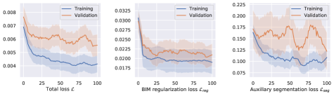
Figure 5: Curves of total loss $\mathcal{L}$, BIM regularization loss $\mathcal{L}_{\text{reg}}$, and auxiliary segmentation loss $\mathcal{L}_{\text{seg}}$ in training and validation, respectively.

We set the ED frame as the moving image and the ES frame as the fixed image in the ACDC and LV quantification datasets in order to estimate cardiac contraction. Each slice in both datasets is cropped to $96\times 96$ with respect to the myocardial centroid after min-max normalization. We compare our proposed framework with several state-of-the-art registration methods including 1) B-splines [13] implemented using SimpleElastix, 2) optical flow [11] implemented using scikit-image registration package, 3) a learning-based registration framework using VAE regularization (RegNet+VAE) [12], and 4) a learning-based registration framework using $\mathcal{L}_{2}$ regularization (RegNet+$\mathcal{L}_{2}$) [4]. The learning-based registration algorithms are implemented using Pytorch with Adam optimizer on 100 epochs. The learning-based models run 18-30 minutes on a single NVIDIA GTX 2080Ti GPU with 12 GB memory for training and validation. The loss curves in training and validation are shown in the supplementary material (Fig. 5). We choose $\nu_{p}=0.4$ (Poisson ratio), $\lambda=0.05$ (weight for BIM loss $\mathcal{L}_{\text{reg}}$), and $\gamma=0.01$ (weight for auxiliary segmentation loss $\mathcal{L}_{\text{seg}}$) in our proposed methods after optimizing hyperparameters. The hyperparameters of the competitor models are optimized as well.

3.3 Evaluation metrics

To evaluate our proposed method, we compute the Dice coefficient (DC), Jaccard index (JD), Hausdorff distance (HD), and average symmetric surface distance (ASD) to evaluate segmentation conformance. We also compute the Jacobian determinant to evaluate the quality of the generated DVF.

4 Results

4.1 Visual and quantitative assessments

Visual assessment of our proposed methods compared to other approaches on the ACDC dataset is shown in Fig. 2. From the figure, we can see that B-splines [13] and optical flow [11] generate artifacts in the myocardium, especially in the highlighted blue patch shown in the third row. The RegNet+VAE [12] creates unrealistic motion in the right ventricle region, especially in the highlighted green patch shown in the last row, which might be due to penalization of the VAE regularizer mainly focusing on the myocardium only. Our proposed methods, in the last two columns, show improved motion compared to the RegNet+$\mathcal{L}_{2}$ with smoother and more biomechanically plausible motion that preserves the geometric features of cardiac structures. The visual results of our proposed methods compared with others on the LV quantification dataset is included in the supplementary material (Fig. 4).

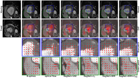
Figure 2: Visual assessment of registration performance on the ACDC 2017 dataset [5].

Method Dice[%]$\uparrow$ Jaccard[%]$\uparrow$ HD[mm]$\downarrow$ ASD[mm]$\downarrow$ LV affine only 72.01 57.24 11.77 2.13 B-splines [13] 89.96 82.62 5.37 0.48 optical flow [11] 87.07 77.87 7.65 0.74 RegNet+VAE [12] 89.61 81.65 6.46 0.49 RegNet+$\mathcal{L}_{2}$ 89.60 81.68 8.00 0.54 RegNet+BIM (ours) 90.32 82.70 5.51 0.37 RegNet+BIM+$\mathcal{L}_{\text{seg}}$ (ours) 92.77 86.76 4.39 0.19 RV affine only 81.08 70.06 14.31 2.21 B-splines [13] 83.59 74.33 13.70 2.43 optical flow [11] 84.96 75.94 13.70 2.15 RegNet+VAE [12] 84.65 75.58 16.48 2.31 RegNet+$\mathcal{L}_{2}$ 84.80 75.73 14.75 2.25 RegNet+BIM (ours) 85.07 76.16 14.55 2.22 RegNet+BIM+$\mathcal{L}_{\text{seg}}$ (ours) 85.93 77.54 14.07 2.15 Epi affine only 85.07 74.50 8.61 0.93 B-splines [13] 92.33 86.12 5.97 0.33 optical flow [11] 92.02 85.64 6.09 0.39 RegNet+VAE [12] 91.45 84.83 7.57 0.48 RegNet+$\mathcal{L}_{2}$ 89.92 82.22 7.77 0.59 RegNet+BIM (ours) 91.53 84.75 6.20 0.40 RegNet+BIM+$\mathcal{L}_{\text{seg}}$ (ours) 92.57 86.48 5.54 0.32

Table 1: Quantitative assessment of registration performance on the ACDC dataset [5].

A quantitative assessment of our proposed methods on the ACDC dataset is reported in Table 1. Our proposed methods outperform other methods in cardiac structures including the LV and epicardium across all evaluation metrics as well as the Jacobian determinant evaluation shown in Table 2. Our methods yield higher conformance in terms of DC and JD in RV and similar performance with B-splines and optical flow in terms of HD and ASD. A quantitative comparison of our proposed method with the others on the LV quantification dataset is included in the supplement (Table  5).

We conduct paired t-tests for statistical significance analysis of our proposed method (RegNet+BIM+$\mathcal{L}_{\text{seg}}$) with the others. Statistically significant improvement ($p<0.05$) is observed for all other methods except for B-splines ($p=0.09$), which might be due to the limited size of the testing set. The complete table is included in the supplementary material (Table 4).

Table 2: Mean Jacobian determinant comparisons on the ACDC 2017 dataset [5].

Method $|\text{det}(J(\hat{u}))-1)|$ B-splines [13] 0.2489 $\pm$ 0.2735 optical flow [11] 0.1283 $\pm$ 0.3432 RegNet+VAE [12] 0.0088 $\pm$ 0.0100 RegNet+$\mathcal{L}_{2}$ 0.0038 $\pm$ 0.0051 RegNet+BIM (ours) 0.0035 $\pm$ 0.0036 RegNet+BIM+$\mathcal{L}_{\text{seg}}$ (ours) 0.0037 $\pm$ 0.0038

4.2 Effect of hyperparameters

To investigate the impact of our proposed biomechanically-informed regularization and the auxiliary segmentation loss, we vary the weights for each loss term as $\lambda=\{0.005,0.05,0.5\}$ and $\gamma=\{0.001,0.01,0.1\}$ and report corresponding LV segmentation performance as shown in Table 3. We also evaluate the effect of Poisson ratio by varying $\nu_{p}=\{0.35,0.4,0.45\}$ in our proposed BIM term. From Table 3, we can see that the $\nu_{p}$ in the vicinity of $0.4$ has little influence on the segmentation conformance. By increasing $\lambda$, we can see that the performance gradually improves from $0.005$ to $0.05$ and deteriorates quite significantly from $0.05$ to $0.5$. This performance loss is likely due to an underestimate of the DVF to avoid a large penalty when trained with a stronger regularization. By increasing $\gamma$, we observe a steady increase in segmentation performance. However, a stronger auxiliary segmentation regularization might yield unrealistic deformation estimates. The structural similarity index between the fixed and moved images for $\gamma=0.01$ to $0.1$ also drops from $0.70$ to $0.65$. We also perform an ablation study to illustrate the effectiveness for each term and the detailed statistics on both datasets are included in the supplementary material (Table 6).

Table 3: Effect of hyperparameters in RegNet+BIM+$\mathcal{L}_{\text{seg}}$ on ACDC 2017 dataset [5]. $\nu_{p}$, $\lambda$, and $\gamma$ denote Poisson ratio, weight for BIM regularization, and weight for $\mathcal{L}_{\text{seg}}$, respectively. By varying each hyperparameter, we report left ventricle segmentation performance.

Parameter $\nu_{p}$ $\lambda$ $\gamma$ Value 0.35 0.4 0.45 0.005 0.05 0.5 0.001 0.01 0.1 Dice[%]$\uparrow$ 92.74 92.77 92.66 91.51 92.77 81.03 91.14 92.77 93.27 Jaccard[%]$\uparrow$ 86.65 86.67 86.56 84.80 86.67 68.72 84.04 86.67 87.54 HD[mm]$\downarrow$ 4.21 4.39 4.51 7.57 4.39 8.25 5.33 4.39 4.17 ASD[mm]$\downarrow$ 0.19 0.19 0.22 0.35 0.19 1.04 0.33 0.19 0.14

5 Discussion

To analyze the potential registration performance among methods for people with different cardiac conditions, we show the Dice score of each method for patients under different pathologies from the ACDC dataset in the boxplot (Fig. 3). From the figure, we can see that our proposed methods yield higher segmentation conformance for dilated cardiomyopathy patients and healthy people. The performance of our proposed methods are similar to others for patients with previous myocardial infarction and hypertrophic cardiomyopathy. Optical flow seems to outperform our proposed method for patients who have abnormal right ventricles. Currently, we validate our proposed methods in the same 2D setting with other competing methods [11, 12].

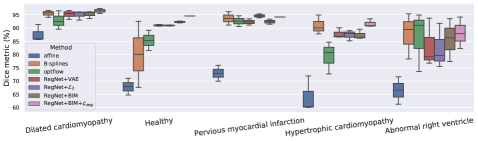
Figure 3: Segmentation conformance in terms of the Dice metric for patients with different pathology from the ACDC dataset [5].

6 Conclusion

In this paper, we propose a data-driven approach for cardiac motion estimation with a novel biomechanics-informed modeling regularization loss. Our proposed methods generate more biomechanically plausible DVFs for all cardiac structures in the image without requiring myocardium segmentation or introducing additional steps compared to network-based regularizers. Our proposed methods outperform other state-of-the-art methods on both the ACDC 2017 dataset and the LV quantification 2019 dataset using quantitative evaluation metrics. Future work will validate current work on other modalities such as tagged MRI and show its effectiveness in more standardized 3D clinical datasets with additional metrics to assess local abnormalities.

Appendix

Figure 4: Visual assessment of registration performance on the LV quantification 2019 dataset [17].

Method Dice[%]$\uparrow$ Jaccard[%]$\uparrow$ HD[mm]$\downarrow$ ASD[mm]$\downarrow$ affine only $p<$0.05 $p<$0.05 $p<$0.05 $p<$0.05 B-splines [13] $p=$0.09 $p=$0.09 $p=$0.09 $p=$0.06 optical flow [11] $p<$0.05 $p<$0.05 $p<$0.05 $p<$0.05 RegNet+VAE [12] $p<$0.05 $p<$0.05 $p<$0.05 $p<$0.05 RegNet+$\mathcal{L}_{2}$ $p<$0.05 $p<$0.05 $p<$0.05 $p<$0.05

Table 4: Analysis of paired t-test for statistical significance between RegNet+BIM+$\mathcal{L}_{\text{seg}}$ (ours) and other methods on the ACDC 2017 dataset [5].

Table 5: Quantitative assessment of registration performance on the LV quantification 2019 dataset [5].

Method Dice[%]$\uparrow$ Jaccard[%]$\uparrow$ HD[mm]$\downarrow$ ASD[mm]$\downarrow$ Endo affine only 82.36 71.14 6.92 0.54 B-splines [13] 84.54 74.30 6.31 0.47 optical flow [11] 83.65 73.01 6.52 0.48 RegNet+VAE [12] 82.70 71.62 6.81 0.52 RegNet+$\mathcal{L}_{2}$ 82.49 71.33 6.91 0.53 RegNet+BIM (ours) 84.24 73.87 6.63 0.48 RegNet+BIM+$\mathcal{L}_{\text{seg}}$ (ours) 86.65 77.48 6.45 0.42 Epi affine only 93.72 88.26 4.62 0.13 B-splines [13] 94.19 89.10 4.27 0.12 optical flow [11] 94.08 88.90 4.33 0.12 RegNet+VAE [12] 93.74 88.29 4.64 0.13 RegNet+$\mathcal{L}_{2}$ 93.72 88.26 4.62 0.13 RegNet+BIM (ours) 93.80 88.41 4.71 0.13 RegNet+BIM+$\mathcal{L}_{\text{seg}}$ (ours) 94.29 89.26 4.50 0.11

Table 6: Ablation study of proposed methods in ACDC 2017 dataset [5] and LV quantification 2019 dataset [17].

Method Dice[%]$\uparrow$ Jaccard[%]$\uparrow$ HD[mm]$\downarrow$ ASD[mm]$\downarrow$ ACDC 2017 Dataset [5] LV RegNet 82.06 70.68 15.45 1.84 RegNet+BIM (ours) 90.32 82.70 5.51 0.37 RegNet+BIM+$\mathcal{L}_{\text{seg}}$ (ours) 92.77 86.76 4.39 0.19 RV RegNet 84.29 75.14 17.15 2.40 RegNet+BIM (ours) 85.07 76.16 14.55 2.22 RegNet+BIM+$\mathcal{L}_{\text{seg}}$ (ours) 85.93 77.54 14.07 2.15 Epi RegNet 86.67 77.06 10.60 0.83 RegNet+BIM (ours) 91.53 84.75 6.20 0.40 RegNet+BIM+$\mathcal{L}_{\text{seg}}$ (ours) 92.57 86.48 5.54 0.32 LV Quantification 2019 Dataset [17] Endo RegNet 84.03 73.58 6.76 0.48 RegNet+BIM (ours) 84.24 73.87 6.63 0.48 RegNet+BIM+$\mathcal{L}_{\text{seg}}$ (ours) 86.65 77.48 6.45 0.42 Epi RegNet 93.71 88.25 4.70 0.13 RegNet+BIM (ours) 93.80 88.41 4.71 0.13 RegNet+BIM+$\mathcal{L}_{\text{seg}}$ (ours) 94.29 89.26 4.50 0.11

References

- [1] Ahn, S.S., Ta, K., Lu, A., Stendahl, J.C., Sinusas, A.J., Duncan, J.S.: Unsupervised motion tracking of left ventricle in echocardiography. In: Medical Imaging 2020: Ultrasonic Imaging and Tomography. vol. 11319, p. 113190Z. International Society for Optics and Photonics (2020)
- [2] Ahn, S.S., Ta, K., Thorn, S., Langdon, J., Sinusas, A.J., Duncan, J.S.: Multi-frame attention network for left ventricle segmentation in 3d echocardiography. In: International Conference on Medical Image Computing and Computer-Assisted Intervention. pp. 348–357. Springer (2021)
- [3] Ashburner, J.: A fast diffeomorphic image registration algorithm. Neuroimage 38(1), 95–113 (2007)
- [4] Balakrishnan, G., Zhao, A., Sabuncu, M.R., Guttag, J., Dalca, A.V.: Voxelmorph: a learning framework for deformable medical image registration. IEEE Transactions on Medical Imaging 38(8), 1788–1800 (2019)
- [5] Bernard, O., Lalande, A., Zotti, C., Cervenansky, F., Yang, X., Heng, P.A., Cetin, I., Lekadir, K., Camara, O., Ballester, M.A.G., et al.: Deep learning techniques for automatic MRI cardiac multi-structures segmentation and diagnosis: Is the problem solved? IEEE Transactions on Medical Imaging 37(11), 2514–2525 (2018)
- [6] Dalca, A.V., Balakrishnan, G., Guttag, J., Sabuncu, M.R.: Unsupervised learning for fast probabilistic diffeomorphic registration. In: International Conference on Medical Image Computing and Computer-Assisted Intervention. pp. 729–738. Springer (2018)
- [7] Gao, Q., Liu, X., Wang, H., Wu, P., Jin, M., Wei, R., Wang, W., Niu, Z., Zhao, S., Li, F.: Optimization of 4d flow mri velocity field in the aorta with divergence-free smoothing. Medical & Biological Engineering & Computing 59(11), 2237–2252 (2021)
- [8] Li, L., Wu, F., Wang, S., Luo, X., Martin-Isla, C., Zhai, S., Zhang, J., Liu, Y., Zhang, Z., Ankenbrand, M.J., et al.: Myops: A benchmark of myocardial pathology segmentation combining three-sequence cardiac magnetic resonance images. arXiv preprint arXiv:2201.03186 (2022)
- [9] Lu, A., Ahn, S.S., Ta, K., Parajuli, N., Stendahl, J.C., Liu, Z., Boutagy, N.E., Jeng, G.S., Staib, L.H., O’Donnell, M., et al.: Learning-based regularization for cardiac strain analysis via domain adaptation. IEEE Transactions on Medical Imaging 40(9), 2233–2245 (2021)
- [10] Papademetris, X., Sinusas, A.J., Dione, D.P., Constable, R.T., Duncan, J.S.: Estimation of 3-d left ventricular deformation from medical images using biomechanical models. IEEE Transactions on Medical Imaging 21(7), 786–800 (2002)
- [11] Pérez, J.S., Meinhardt-Llopis, E., Facciolo, G.: Tv-l1 optical flow estimation. Image Processing On Line 2013, 137–150 (2013)
- [12] Qin, C., Wang, S., Chen, C., Qiu, H., Bai, W., Rueckert, D.: Biomechanics-informed neural networks for myocardial motion tracking in MRI. In: International Conference on Medical Image Computing and Computer-Assisted Intervention. pp. 296–306. Springer (2020)
- [13] Rueckert, D., Sonoda, L.I., Hayes, C., Hill, D.L., Leach, M.O., Hawkes, D.J.: Nonrigid registration using free-form deformations: application to breast MR images. IEEE Transactions on Medical Imaging 18(8), 712–721 (1999)
- [14] Sang, Y., Ruan, D.: Enhanced image registration with a network paradigm and incorporation of a deformation representation model. In: 2020 IEEE 17th International Symposium on Biomedical Imaging (ISBI). pp. 91–94. IEEE (2020)
- [15] Sang, Y., Ruan, D.: 4d-cbct registration with a fbct-derived plug-and-play feasibility regularizer. In: International Conference on Medical Image Computing and Computer-Assisted Intervention. pp. 108–117. Springer (2021)
- [16] Spencer, A.J.M.: Continuum mechanics. Courier Corporation (2004)
- [17] Xue, W., Brahm, G., Pandey, S., Leung, S., Li, S.: Full left ventricle quantification via deep multitask relationships learning. Medical Image Analysis 43, 54–65 (2018)
- [18] You, C., Dai, W., Staib, L., Duncan, J.S.: Bootstrapping semi-supervised medical image segmentation with anatomical-aware contrastive distillation. arXiv preprint arXiv:2206.02307 (2022)
- [19] You, C., Xiang, J., Su, K., Zhang, X., Dong, S., Onofrey, J., Staib, L., Duncan, J.S.: Incremental learning meets transfer learning: Application to multi-site prostate mri segmentation. arXiv preprint arXiv:2206.01369 (2022)
- [20] You, C., Yang, J., Chapiro, J., Duncan, J.S.: Unsupervised wasserstein distance guided domain adaptation for 3d multi-domain liver segmentation. In: Interpretable and Annotation-Efficient Learning for Medical Image Computing, pp. 155–163. Springer (2020)
- [21] You, C., Zhao, R., Liu, F., Chinchali, S., Topcu, U., Staib, L., Duncan, J.S.: Class-aware generative adversarial transformers for medical image segmentation. arXiv preprint arXiv:2201.10737 (2022)
- [22] You, C., Zhao, R., Staib, L., Duncan, J.S.: Momentum contrastive voxel-wise representation learning for semi-supervised volumetric medical image segmentation. arXiv preprint arXiv:2105.07059 (2021)
- [23] You, C., Zhou, Y., Zhao, R., Staib, L., Duncan, J.S.: Simcvd: Simple contrastive voxel-wise representation distillation for semi-supervised medical image segmentation. IEEE Transactions on Medical Imaging (2022)
- [24] Zhang, X., Li, Y., Liu, Y., Tang, S.X., Liu, X., Punithakumar, K., Shi, D.: Automatic spinal cord segmentation from axial-view mri slices using cnn with grayscale regularized active contour propagation. Computers in Biology and Medicine 132, 104345 (2021)
- [25] Zhang, X., Martin, D.G., Noga, M., Punithakumar, K.: Fully automated left atrial segmentation from mr image sequences using deep convolutional neural network and unscented kalman filter. In: 2018 IEEE International Conference on Bioinformatics and Biomedicine (BIBM). pp. 2316–2323. IEEE (2018)
- [26] Zhang, X., Noga, M., Martin, D.G., Punithakumar, K.: Fully automated left atrium segmentation from anatomical cine long-axis mri sequences using deep convolutional neural network with unscented kalman filter. Medical Image Analysis 68, 101916 (2021)
- [27] Zhang, X., Noga, M., Punithakumar, K.: Fully automated deep learning based segmentation of normal, infarcted and edema regions from multiple cardiac mri sequences. In: Myocardial Pathology Segmentation Combining Multi-Sequence CMR Challenge. pp. 82–91. Springer (2020)