Statistical validation of the detection of a sub-dominant quasi-normal mode in GW190521

Abstract

One of the major aims of gravitational wave astronomy is to observationally test the Kerr nature of black holes. The strongest such test, with minimal additional assumptions, is provided by observations of multiple ringdown modes, also known as black hole spectroscopy. For the gravitational wave merger event GW190521, we have previously claimed the detection of two ringdown modes emitted by the remnant black hole. In this paper we provide further evidence for the detection of multiple ringdown modes from this event. We analyse the recovery of simulated gravitational wave signals designed to replicate the ringdown properties of GW190521. We quantify how often our detection statistic reports strong evidence for a sub-dominant $(\ell,m,n)=(3,3,0)$ ringdown mode, even when no such mode is present in the simulated signal. We find this only occurs with a probability $\sim 0.02$, which is consistent with a Bayes factor of ${56\pm 1}{}$ (1$\sigma$ uncertainty) found for GW190521. We also quantify our agnostic analysis of GW190521, in which no relationship is assumed between ringdown modes, and find that only 1 in 250 simulated signals without a $(3,3,0)$ mode yields a result as significant as GW190521. Conversely, we verify that when simulated signals do have an observable $(3,3,0)$ mode they consistently yield a strong evidence and significant agnostic results. We also find that constraints on deviations from the $(3,3,0)$ mode on GW190521-like signals with a $(3,3,0)$ mode are consistent with what was obtained from our previous analysis of GW190521. Our results strongly support our previous conclusion that the gravitational wave signal from GW190521 contains an observable sub-dominant $(\ell,m,n)=(3,3,0)$ mode.

I Introduction

Einstein’s theory of general relativity (GR) predicts that black holes are stable to perturbations Andersson et al. (2019). A distorted black hole should settle down to a stationary Kerr state through the emission of gravitational waves Whiting (1989). This applies to the remnant black hole formed in a binary black hole merger event, which is highly distorted on formation, but is expected to eventually settle down to a Kerr black hole due to the emission of gravitational waves. The gravitational waveform in the late stages of a merger event consists of a spectrum of quasi-normal modes with a rich structure of different fundamental modes and overtones Berti et al. (2009). The spectrum consists of a set of complex frequencies (determined by the black hole mass and spin) labeled by three integers $(\ell,m,n)$, with $\ell\geq 2$, $-\ell\leq m\leq\ell$, and $n\geq 0$. Modes with $n\geq 1$ are known as “overtones”. Using black hole spectroscopy, the observation of more than one such ringdown mode can be used to determine if the black hole is consistent with GR Dreyer et al. (2004); Kamaretsos et al. (2012). A clear and unambiguous determination of multiple ringdown modes provides one of the strongest tests of the Kerr nature of black holes in our universe and a possible route to discover new physics beyond standard general relativity.

Quasi-normal modes for a Schwarzschild black hole were first identified by Vishveshwara Vishveshwara (1970a, b), and further studied within black hole perturbation theory by Chandrasekhar and Detweiler Chandrasekhar and Detweiler (1975). There remain several outstanding theoretical questions regarding black hole quasi-normal modes which are also important for observational studies. The first is the question of the start time for the ringdown. When the remnant black hole is formed, it is initially highly distorted away from a Kerr black hole. The black hole loses these distortions over time, and at some point it can be considered to be a linear perturbation of a Kerr black hole. It is not clear when (and if Thrane et al. (2017)) this perturbative regime can be distinguished. See Kamaretsos et al. (2012); Bhagwat et al. (2018) for studies of the start time of the ringdown phase, and Okounkova (2020); Mitman et al. (2022); Lagos and Hui (2022); Cheung et al. (2022) for studies of possible non-linear effects. The different regimes seen in the gravitational wave signal are expected to have counterparts in the strong field dynamical spacetime region near the binary system Jaramillo et al. (2012a, b); Prasad et al. (2020). See e.g. Mourier et al. (2021); Forteza and Mourier (2021); Pook-Kolb et al. (2020); Gupta et al. (2018); Chen et al. (2022) for studies of black hole horizon geometry in the post-merger phase and whether a ringdown regime can be identified using the horizon dynamics as well.

It has long been expected that only the most dominant ringdown mode will be observable with the current generation of gravitational wave detectors Berti et al. (2016); Cabero et al. (2020). Those expectations were based on astrophysical assumptions about the total mass and mass ratio distributions of binary black hole systems in the observable universe, which in turn determine the amplitudes of various ringdown modes Borhanian et al. (2020). However, evidence for an overtone of the dominant mode of GW150914 was presented in Isi et al. (2019); Giesler et al. (2019). There it was shown that it is possible to model the gravitational waveform as a superposition of ringdown modes starting from the merger by using the overtones of the dominant mode. This is a significant result, though there remain several interesting open questions regarding data analysis and theoretical issues. Some of the data analysis issues are discussed in Cotesta et al. (2022); Isi and Farr (2022). On the theoretical side, the stability of the overtones under small perturbations raises several interesting open questions; see e.g. Nollert (1996); Nollert and Price (1999); Jaramillo et al. (2021, 2022); Destounis et al. (2021). Evidence of a second fundamental mode, without using overtones, was first presented for the event GW190521 in Capano et al. (2021), henceforth referred to as “Capano et al.”, and will be elaborated further in this paper.

With this analysis we address three fundamental questions. Firstly, if a signal explicitly does not contain any sub-dominant ringdown modes, how often does our detection pipeline falsely claim the existence of such modes? Secondly, if one or more sub-dominant modes are present in the data, how often does our pipeline correctly recover them? Thirdly, if our pipeline is used to constrain deviations from Kerr, how well do the resulting inferred parameters match those of the simulated signal? The key results for detection of a second mode are shown in Figs. 4 and 5. Figure 4 shows the result of applying the “agnostic analysis” performed in Capano et al. to a set of simulated signals that do not have a $(3,3,0)$ mode as compared to a set that do. Figure 5 (left) applies the “Kerr analysis” from Capano et al. to simulated signals without a $(3,3,0)$ mode, and shows that the false alarm probability is consistent with expectations from noise. Figure 5 (right) quantifies the ability of the Kerr analysis to detect the $(3,3,0)$ mode when it is present, as a function of the signal strength.

In section II we give additional details of how the data is treated in the analysis of Capano et al. Section III explains how we generate the simulated data sets. In sections IV and V we investigate the statistical significance of detecting two modes versus one using a set of simulated signals. Section IV presents an agnostic analysis that looks at the consistency of the second mode with the first mode. Section V presents an analysis more closely tied to the Kerr hypothesis, analysing the likelihood of two Kerr modes versus just one. In section VI we use our simulated signals to compare the accuracy with which the no hair theorem can be tested using fundamental modes or overtones for an event similar to GW190521.

We conclude this introduction by briefly summarizing some basic properties of the event GW190521, which will be relevant in the rest of this paper.

I.1 GW190521

The gravitational wave event GW190521 was detected on May 21st 2019 at 03:02:29 UTC by the Advanced LIGO and Advanced Virgo detectors Abbott et al. (2020a). The most conservative explanation of the signal is the binary merger of two black holes Abbott et al. (2020a, b), although there are also various other interpretations of this event Bustillo et al. (2021); Abedi et al. (2021); Wang et al. (2022); Gamba et al. (2021); Dall’Amico et al. (2021); Shibata et al. (2021).

While the progenitors of the event GW190521 are open to speculation, in most scenarios the final outcome is still likely to be a single black hole. The event GW190521 shows clear evidence of a dominant ringdown mode of a final black hole after the merger Abbott et al. (2020a). In Capano et al. Capano et al. (2021) the ringdown signal was found to contain an additional sub-dominant ringdown mode. The dominant mode is consistent with being the $(\ell,m,n)=(2,2,0)$ ringdown mode of a Kerr black hole; the second mode is consistent with the sub-dominant fundamental $(\ell,m,n)=(3,3,0)$ mode. As detailed in this paper, under a Kerr hypothesis, the Bayes factor preferring the existence of the $(2,2,0)$ and $(3,3,0)$ modes over just the $(2,2,0)$ or the $(2,2,0)$ and $(2,2,1)$ modes is estimated to be ${56\pm 1}{}$ (1$\sigma$ uncertainty).

If GW190521 is indeed a binary black hole merger, the inferred total mass of the system would make it one of the most massive binary black hole systems observed to date Abbott et al. (2021a); Nitz et al. (2021a). Other interpretations have found even higher total masses Bustillo et al. (2021). A high total mass implies that very little of the inspiral phase occurs inside the sensitive band of the detectors and the recorded signal is dominated by the merger and ringdown. Therefore an analysis that focuses solely on the ringdown phase is of interest and avoids some of the modelling issues in the progenitor inspiral phase.

Inferences about the final black hole parameters using the ringdown signal alone are sensitive to the assumed start time of the ringdown Kamaretsos et al. (2012); Cotesta et al. (2022). Different starting times can lead to different results Cabero et al. (2018); Kastha et al. (2022). A ringdown-only analysis must explicitly exclude some of the signal that is outside the ringdown phase. In this work we present additional details of the approach used in Capano et al. Parameter estimates for the event GW190521 based on the binary black hole interpretation are shown in Figs. 1 and 2. These estimates come from different authors using different methods Nitz and Capano (2021); Estellés et al. (2022); Capano et al. (2021); Nitz et al. (2021a). The redshifted final total mass spans a wide range from around $200~{}\mathrm{M}_{\odot}$ to nearly $400~{}\mathrm{M}_{\odot}$.

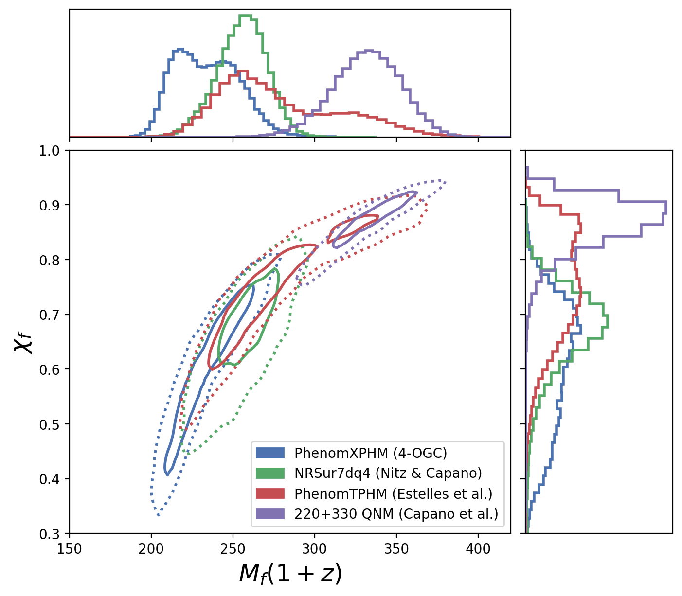
Figure 1: Comparison of the final mass and spin of GW190521, as estimated by NRSur7dq4 Nitz and Capano (2021), IMRPhenomXPHM Nitz et al. (2021a), IMRPhenomTPHM Estellés et al. (2022), and a Kerr ringdown with both the $(2,2,0)$ and $(3,3,0)$ modes Capano et al. (2021). The solid and dashed lines correspond to $50\%$ and $90\%$ credible contour, respectively. The IMRPhenomTPHM results have a second mode in the posterior that is consistent with the Kerr ringdown results.

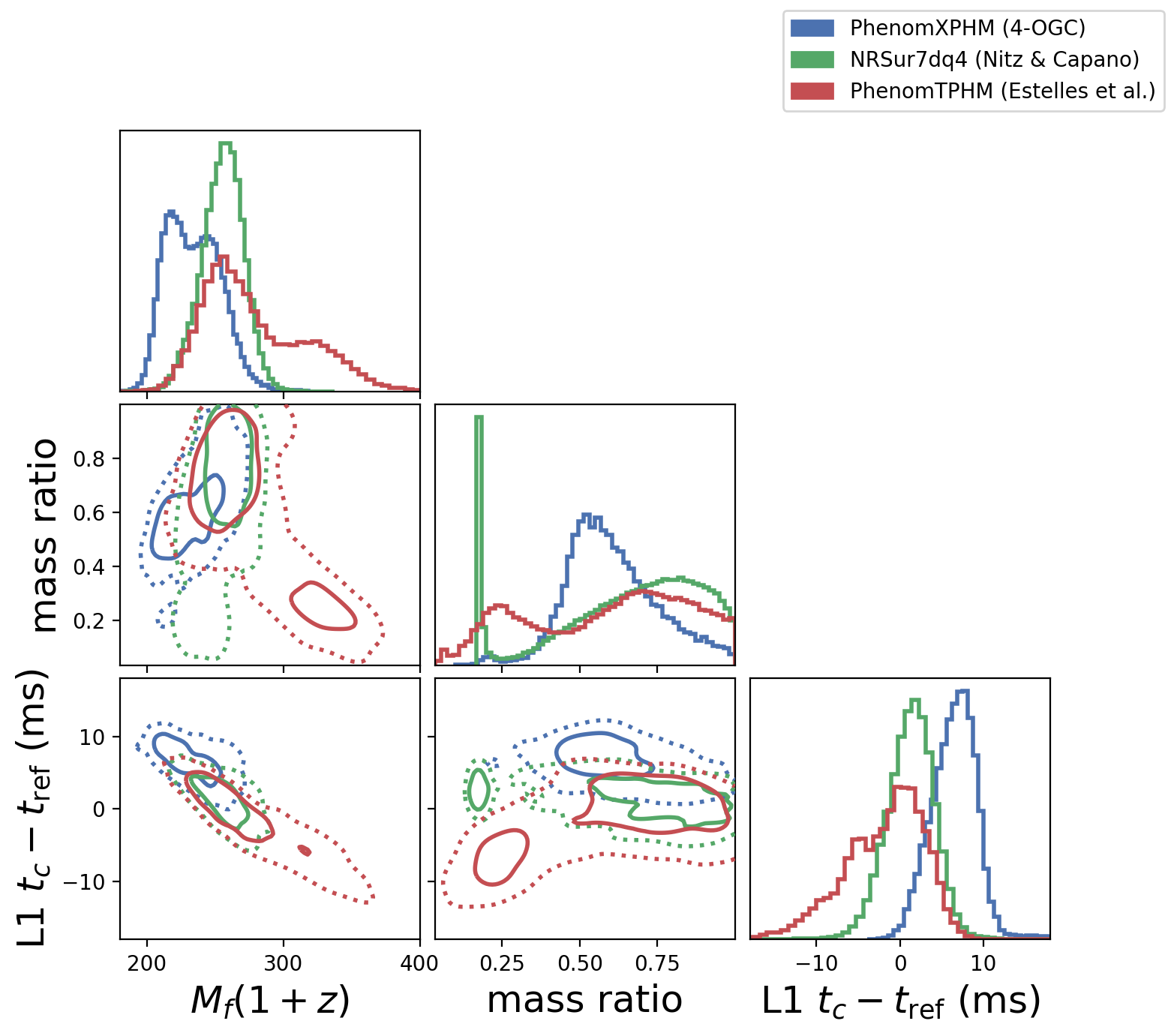
Figure 2: Comparison of the final mass, mass ratio, and coalescence time in the Livingston detector as estimated by the NRSur7dq4 Nitz and Capano (2021), IMRPhenomXPHM Nitz et al. (2021a), and IMRPhenomTPHM Estellés et al. (2022) waveform models. The solid and dashed lines correspond to $50\%$ and $90\%$ credible contour, respectively. The second mode in final mass found by IMRPhenomTPHM, which is consistent with the Kerr ringdown results (cf. Fig. 1), corresponds to a second mode at more asymmetric masses. This mode also yields a coalescence time that is $\sim 6\,$ms earlier than the equal mass mode found by the other approximants. This earlier coalescence time estimate is $\sim 12\,$ms before the time at which the Bayes factor for the $(2,2,0)+(3,3,0)$ mode peaks in Capano et al. Capano et al. (2021). It is also consistent with the time at which the evidence for the $(2,2,0)+(2,2,1)$ Kerr ringdown model peaks.

The peak gravitational wave strain is expected to occur close to the merger. The GPS time of the peak strain in the Hanford detector was initially estimated by the LIGO Scientific and Virgo Collaborations (LVC) using a numerical relativity (NR) surrogate waveform model, NRSur7dq4 Varma et al. (2019), to be $1242442967.4306^{+0.0067}_{-0.0106}$ (median $\pm 90\%$ credible interval) Abbott et al. (2020b). See Estellés et al. (2022) for further discussion. As can be seen in Fig. 2, estimates of the merger coalescence time range over some $20\,$ms depending on the waveform model considered. This is a significant time range since, in geometric units, it corresponds to approximately $13M$ for an object with a mass $M=300~{}\mathrm{M}_{\odot}$. For this reason, in Capano et al. a range of starting times for the ringdown analysis was used, which spans the uncertainty of merger time estimation. See Section III for more details.

II Basics of ringdown detection and parameter estimation

In this section we summarize some essential elements of the data analysis procedure that we employ. Since we analyze exclusively the ringdown which is only a part of the full signal, an important challenge is to identify the portion of the full signal corresponding to the ringdown. Similarly, it is necessary to ensure that the procedure for extracting this portion of the data properly takes into account correlations with neighboring time samples that should be excluded from the analysis.

Let $\vec{s}=\{s_{0},...,s_{N-1}\}$ denote time-ordered samples of the strain data from a gravitational wave detector. The data is sampled every $\Delta t$ seconds over a duration $T$, so that the number of samples is $N=\lfloor T/\Delta t\rfloor+1$. A network of $K{}$ detectors sampled in this way will produce a set of samples $\vec{s}_{\mathrm{net}}=\{\vec{s}_{1},...,\vec{s}_{K}\}$. The strain data is assumed to be a combination of a possible signal $\vec{h}$ and noise $\vec{n}$

$$\vec{s}=\vec{h}+\vec{n}\,.$$ (1)

Let $p(\vec{s}|\vec{\lambda},H)$ be the likelihood of the data $\vec{s}$ in the presence of a signal with given parameters $\vec{\lambda}$ under background hypotheses $H$, such as the signal model. The probability of finding a realisation of noise $\vec{n}$ under the hypotheses $H$ is $p(\vec{n}|H)$. Therefore the likelihood for data $\vec{s}$ can be written as

$$p(\vec{s}|\vec{\lambda},H)=p(\vec{s}-\vec{h}(\vec{\lambda})|H,n)\,,$$ (2)

where the right-hand side is under the hypothesis $n$ that no signal is present. In gravitational-wave astronomy, in the absence of a signal, it is common to assume over short times that the detectors output stochastic Gaussian noise which is independent across detectors. With this assumption the probability density function describing the time-ordered noise samples of the detector network $\vec{n}_{\mathrm{net}}$ is a product of $K{}$ $N-$dimensional multivariate normal distributions,

$$p(\vec{n}_{\mathrm{net}})=\frac{\exp\left[-\frac{1}{2}\sum_{d=1}^{K{}}\vec{n}_{d}^{\top}\vec{C}_{d}^{-1}\vec{n}_{d}\right]}{\sqrt{(2\pi)^{NK{}}\prod_{d=1}^{K{}}\det\vec{C}_{d}}}.$$ (3)

Here, $\vec{C}_{d}$ is the covariance matrix of the noise in detector $d$, and we drop the hypotheses $H$ in our notation. See Finn (1992) for further details.

If the detector’s noise is wide-sense stationary and ergodic, which is typically the case for the LIGO and Virgo detectors, the noise likelihood takes a simple form

$$p(\vec{n}_{\mathrm{net}})\propto\exp\left[-\frac{1}{2}\sum_{d=1}^{K}\left<\vec{n}_{d},\vec{n}_{d}\right>\right].$$ (4)

Here, the inner product $\left<\cdot,\cdot\right>$ is defined as

$$\left<\vec{u}_{d},\vec{v}_{d}\right>\equiv 4\Re\left\{\frac{1}{T}\sum_{p=1}^{N/2-1}\frac{\tilde{u}_{d}^{*}[p]\tilde{v}_{d}[p]}{S_{n}^{(d)}[p]}\right\},$$ (5)

where $\tilde{u}$ is the discrete Fourier transform of the time series $\vec{u}$, an asterisk denotes the complex conjugate, and $S_{n}$ is the power spectral density of the detector’s noise. To obtain the posterior probability density function $p(\vec{\lambda}|\vec{s},H)$ for the parameters $\vec{\lambda}$, we use Bayes’ theorem

$$p(\vec{\lambda}|\vec{s},H)=\frac{1}{Z}p(\vec{s}|\vec{\lambda},H)p(\vec{\lambda}|H),$$ (6)

where $p(\vec{s}|\vec{\lambda},H)$ is the likelihood function, $p(\vec{\lambda}|H)$ is the prior, and $Z$ is a normalization constant known as the evidence, depending only on the data. Taking the ratio of evidences $Z_{A}/Z_{B}$ for two different models $H_{A}$ and $H_{B}$ yields the “Bayes factor”. In this work, the signal models will be GW ringdown waveforms with only fundamental modes and overtones. If our prior belief for the validity of the two models is the same, the Bayes factor gives the odds that model A is favoured over model B. Ref. Kass and Raftery (1995) suggested Bayes factors greater than 3.2, 10 and 100 are considered substantial, strong, and decisive, respectively.

The ringdown waveform model takes the following form

$$h_{+}+ih_{\times}={\displaystyle\frac{M_{f}}{D_{L}}}\sum_{{\ell mn}}{}_{{}_{-2}}S_{{\ell mn}}(\iota,\varphi,{\chi}_{f})A_{{\ell mn}}e^{i(\Omega_{{\ell mn}}t+\phi_{{\ell mn}})}\,,$$ (7)

where $h_{+/\times}$ are the plus/cross polarizations of the wave, $M_{f}$ is the total mass of the remnant black hole in the detector frame and $D_{L}$ is the source luminosity distance. The waveform is decomposed with respect to the spin-2 weighted spheroidal basis ${}_{{}_{-2}}S_{{\ell mn}}$, which is a function of the remnant black hole’s spin $\chi_{f}$, the inclination angle $\iota$ and azimuthal angle $\varphi$ relative to the observer. The amplitude and phase of the quasi-normal modes are denoted by $A_{{\ell mn}}$ and $\phi_{{\ell mn}}$. The complex frequency is $\Omega_{{\ell mn}}=2\pi f_{{\ell mn}}+i/\tau_{{\ell mn}}$, where the characteristic frequency $f_{{\ell mn}}$ and decay time $\tau_{{\ell mn}}$ are solely determined by the mass and spin of the remnant black hole, as predicted by the no-hair theorem in GR. We also consider an agnostic ringdown waveform model in this work, for which we absorb the $M_{f}/D_{L}$ term into the amplitude and replace the spheroidal harmonics with arbitrary complex numbers $X_{\ell\pm mn}=e^{i\psi_{\ell\pm mn}}$.

In a standard full-signal analysis, to obtain the likelihood for the signal hypothesis, the noise $\vec{n}_{d}$ in Eq. 4 is replaced by the residuals $\vec{s}_{d}-\vec{h}_{d}$. This requires that $\vec{h}$ is an accurate model of the signal across the entire observation time $T$, which is not valid for a ringdown-only analysis. Quasi-normal modes only model the gravitational wave from a binary black hole after the merger, when the two component black holes have formed a single, perturbed black hole. Performing Bayesian inference using quasi-normal modes as the signal model therefore requires ignoring times from the data when the ringdown prescription is not valid.

We perform the “gating and in-painting” technique Zackay et al. (2021) to remove the influence of pre-ringdown data. Define $\vec{n}^{\prime}=\vec{n}_{g}+\vec{x}$, where $\vec{n}_{g}$ is the noise with the pre-merger data zeroed out. We solve for $\vec{x}$ such that $\vec{C}^{-1}\vec{n}^{\prime}=0$ in the gated region. Doing so, we can use $\vec{n}^{\prime}$ in the frequency-domain likelihood equation Eq. 4 to obtain the same result as if we excised the gated time and directly computed the likelihood in Eq. 3.

We use the gated-Gaussian likelihood described above in the open source PyCBC Inference library Nitz et al. (2021b); Biwer et al. (2019). We evaluate the noise residuals with $\vec{n}_{g}=\vec{s}_{g}-\vec{h}_{g}$ (i.e., the residual with the gated region zeroed out) and solve for $\vec{x}$ under the condition

$$\overline{\vec{C}^{-1}}\,\overline{\vec{x}}=-\overline{\vec{C}^{-1}\vec{n}_{g}},$$ (8)

where the overbar indicates the gated region. We can then use $\vec{x}+\vec{s}_{g}-\vec{h}_{g}$ in the standard likelihood, Eq. 4.

For all analyses we use a gate of two seconds, ending at the start time of the ringdown. We use data for the event GW190521 made publicly available by the Gravitational Wave Open Science Center Abbott et al. (2021b). For all injections we fix the sky location to the values given by the maximum likelihood result of Nitz & Capano Nitz and Capano (2021). For sampling the parameter space we use the dynesty nested sampler Speagle (2020).

In this work we consider a variety of signal models with different combinations of angular and overtone modes characterized by Eq. 7. The fundamental mode is $(\ell,m,n)=(2,2,0)$, and we further consider models with an additional $(2,2,1)$ overtone or $(3,3,0)$ mode, whose complex frequencies are either predicted by the Kerr hypothesis or treated agnostically as parameters to be determined. We list the priors $p(\vec{\lambda}|H)$ for all parameters used in this work in Table 1. In particular, the (2,2,1) amplitude is chosen to be [0,5] times that of the (2,2,0) mode’s. This choice is motivated by the numerical relativity fits from Giesler et al. (2019), and helps to prevent “label switching” in which the (2,2,1) mode template matches to the fundamental mode signal in the data. For the $(3,3,0)$ amplitude we chose a prior that is $[0,0.5]$ times that of the (2,2,0) mode, which is informed by the numerical simulation results of binary black hole mergers in Ref. Borhanian et al. (2020).

When sampling the posterior for the Kerr and agnostic analysis, we numerically marginalize the polarization angle using a discrete grid of 1000 points. The original motivation was to speed up sampler convergence for the large number of injections analyzed here. However, we found that doing so also led to more robust estimates of the Bayesian evidence, as the sampler was better able to converge on the posterior. Consequently we also reanalyzed GW190521 using the numerical marginalization of the polarization. The effect on the estimation of the Bayes factor is discussed in more detail in Appendix A.

Model	Parameter	Parameter description	Uniform prior range
	$f_{A/B/C}$	frequencies of regions A/B/C	$[50,80]$/$[80,256]$/$[15,50]$ Hz
	$\tau_{A/B/C}$	decay times of regions A/B/C	$[0.001,0.1]$ s
	$\log_{10}A_{B}$	base-10 logarithm of the amplitude of region B	[-24,19]
Agnostic	$A_{A/C}/A_{B}$	ratio of amplitudes between region A/C and region B	[0,0.9]
	$\phi_{A/B/C}$	phases of regions A/B/C	$[0,2\pi]$
	$\psi^{+/-}_{A/B/C}$	phase of the +m and -m modes of the arbitrary complex number in region A/B/C	$[0,2\pi]$
	$d\beta$	angular difference in amplitudes of +m and -m modes	$[-\pi/4,\pi/4]$
	$M_{f}$	final black hole mass in the detector frame	[100,500] $M_{\odot}$
	$\chi_{f}$	final black hole spin	[-0.99,0.99]
Kerr	$\log_{10}A_{220}$	base-10 logarithm of the amplitude of (2,2,0)	[-24,-19]
	$A_{330/220}$	ratio of amplitudes between $(3,3,0)$ and $(2,2,0)$	[0,0.5]
	$A_{221/220}$	ratio of amplitude between $(2,2,1)$ and $(2,2,0)$	[0,5]
	$\phi_{220/330/221}$	phase of (2,2,0)/(2,2,1)/(3,3,0)	$[0,2\pi]$
	$\delta f_{221}$	fractional deviation from GR of the (2,2,1) frequency	[-0.16,0.3] with the constraint $f_{221}(1+\delta f_{221})>55$ Hz
No hair test	$\delta\tau_{221}$	fractional deviation from GR of the (2,2,1) decay time	[-0.8,0.8]
	$\delta f_{330}$	fractional deviation from GR of the $(3,3,0)$ frequency	[-0.3,0.3] with the constraint $f_{330}(1+\delta f_{330})>75$ Hz
	$\delta\tau_{330}$	fractional deviation from GR of the $(3,3,0)$ decay time	[-0.9,3]
All models	$\cos\iota$	cosine of inclination angle	[-1,1]
	$\psi$	polarization angle	$[0,2\pi]$

Table 1: Prior distributions of sampling parameters for the models used in this work: The agnostic model with the spheroidal harmonics replaced by an arbitrary complex number as discussed in Sec. IV, the Kerr model described by Eq. 7 and discussed in Sec. V, and the testing-GR model discussed in Sec. VI.

III Selection of simulated signals

In this paper we seek to validate the evidence for the observation of the $(3,3,0)$ mode in GW190521. To do so, we create two sets of simulated signals (“injections”): one set with no $(3,3,0)$ mode in the ringdown (the Control set), and another set containing a $(3,3,0)$ mode in the ringdown (the Signal set). The Control set is used to measure the rate of false alarms – i.e., to answer the question, how often do we get large evidence for the $(3,3,0)$ mode when the signal contains no $(3,3,0)$ mode? – while the Signal set is used to validate that our pipeline can in fact detect a $(3,3,0)$ mode when it exists in the signal.

For the Control injections we randomly select 500 points from the NRSurrogate posterior published in Nitz & Capano Nitz and Capano (2021). This posterior was similar to the posterior published in the initial LIGO/Virgo publication on GW190521 Abbott et al. (2020b). With the exception of a secondary peak in the posterior around $m_{1}/m_{2}\sim 6$, this NRSurrogate posterior favored approximately equal masses for the binary. It also yielded a merger time for GW190521 only $\sim 6\,$ms before the claimed observation time of the $(3,3,0)$ mode in Capano et al. and a relatively low final mass estimate; see Figs. 1 and 2. These results contrast with the claimed observation in Capano et al.: a large $(3,3,0)$ amplitude is not expected for equal-mass binaries Borhanian et al. (2020), and a ringdown model consisting of only fundamental modes is not expected to be a good model for the signal until $\sim 10\,M$ after merger, which for GW190521 would be $\sim 12-16\,$ms, not $\sim 6\,$ms. As such, these injections are ideal to test the false alarm rate of our analyses.

To ensure that no $(3,3,0)$ mode exists in the Control injections, we constrain all 500 injections to have mass ratios $m_{2}/m_{1}>0.5$ and we turn off all but the $\ell=2$ modes when generating the simulated waveforms. The waveforms are generated using the NRSur7dq4 approximant Varma et al. (2019). We use 500 injections to get a sufficient number of samples at the Bayes factor of GW190521 ($56\pm 1$); see Sec. V for more details.

To produce the Signal injections we draw random samples from the posterior published in Estelles et al. Estellés et al. (2022). This analysis used the IMRPhenomTPHM approximant to analyze GW190521. As with the results presented in Nitz & Capano Nitz and Capano (2021), Estelles et al. found a bimodal posterior in the component masses for GW190521: one mode favoring nearly equal masses, and one mode favoring mass ratios of $\sim 4:1$. Intriguingly, as shown in Figs. 1 and 2, the second mode yielded a mass and spin estimate for the final black hole that is consistent with the estimate from the ringdown analysis in Capano et al. The estimated merger time for this second mode was also $\sim 5-10\,$ms earlier than the NRSurrogate estimate, which is consistent with the peak in the $(2,2,1)$ Bayes factor found in Capano et al. and $\sim 10\,M$ before the peak in the $(3,3,0)$ Bayes factor. The IMRPhenomTPHM waveforms are therefore ideal for our Signal injection set, particularly those from the more asymmetric mass ratio part of the posterior.

To try to ensure that the Signal injections have an observable $(3,3,0)$ mode after the merger, we draw 100 injections from the IMRPhenomTPHM posterior published in Estelles et al. and keep only those that have an estimated $(\ell,m,n)=(3,3,0)$ amplitude $>0.2$ after merger. We also require that the signal-to-noise ratio (SNR) of the $(3,3,0)$ mode be at least $4$ (the SNR estimated for the $(3,3,0)$ mode in GW190521 in Capano et al.) at some point after merger. To estimate the $(3,3,0)$ SNR we filter each injection in noise with a template consisting only of the $(\ell,m)=(3,3)$ mode, and we gate both the template and signal to remove pre-merger times. Note that here, $(\ell,m)$ refer to spherical harmonics, which is the basis used for inspiral-merger-ringdown (IMR) models, not the spheroidal harmonics used for QNMs. Many of the posterior samples have large precession. Precession mixes the $m$ modes with the same $\ell$ in the observer frame. Consequently, an $(\ell,m)=(3,3)$ mode for a IMRPhenomTPHM waveform may consist of a combination of $(\ell,m,n)$ QNM modes, and not necessarily just the $(3,3,0)$ mode. As such, the estimated SNR may be considered an upper bound on the underlying $(3,3,0)$ QNM.

Applying the SNR cut to the initial 100 draws yields 45 Signal injections. We do not try to generate more Signal injections as they are only used to check that the analysis can recover signals with a $(3,3,0)$ mode and not to estimate small false alarm rates, as we do with the Control injections. We use IMRPhenomTPHM to generate the waveform for the Signal set. Due to the differences between spherical and spheroidal modes, and to try to simulate a realistic signal, we use all available modes in IMRPhenomTPHM when generating the Signal set.

Both sets of injections are added to detector data at random times surrounding the estimated merger time of GW190521. Specifically, an offset time $t_{\rm offset}$ is drawn uniformly in $\pm[4,20]\,$s and added to the coalescence time $t_{c}$ that is drawn from the relevant posterior for each injection. The gap of $\pm 4\,$s around GW190521 is to prevent contamination of the data from GW190521. As described below, we perform ringdown analyses on a grid of times surrounding each injection. The widest grid – used in the validation of the Kerr Bayes factor (see Sec. V) – is $[-9,24]\,$ms. We therefore draw the $t_{\rm offset}$ such that they are at least $33\,$ms apart, to ensure that no two analyses analyze exactly the same detector data.

As with the analysis of GW190521 in Capano et al., we use a reference time $t^{\rm inj}_{\rm ref}$ for each injection, around which we construct the grid of times used in the ringdown analyses. For each injection we set the reference time to be $t^{\rm inj}_{\rm ref}=t_{\rm ref}+t_{\rm offset}$, where $t_{\rm ref}=1242442967.445$ GPS seconds is the estimated geocentric merger time of GW190521, as determined by the maximum likelihood parameters taken from the NRSurrogate analysis in Nitz & Capano Nitz and Capano (2021). This is the same $t_{\rm ref}$ used in Capano et al. Note that $t^{\rm inj}_{\rm ref}$ is not the injection’s coalescence time $t^{\rm inj}_{c}$; instead, $t^{\rm inj}_{c}-t^{\rm inj}_{\rm ref}$ follow the same distribution as $t_{c}-t_{\rm ref}$ (see Fig. 2). In the case of IMRPhenomTPHM, this can mean that some of our Signal injections merge as much as $20\,$ms before the reference time, well before the grid times used for the analysis.

IV Statistical significance of the agnostic analysis

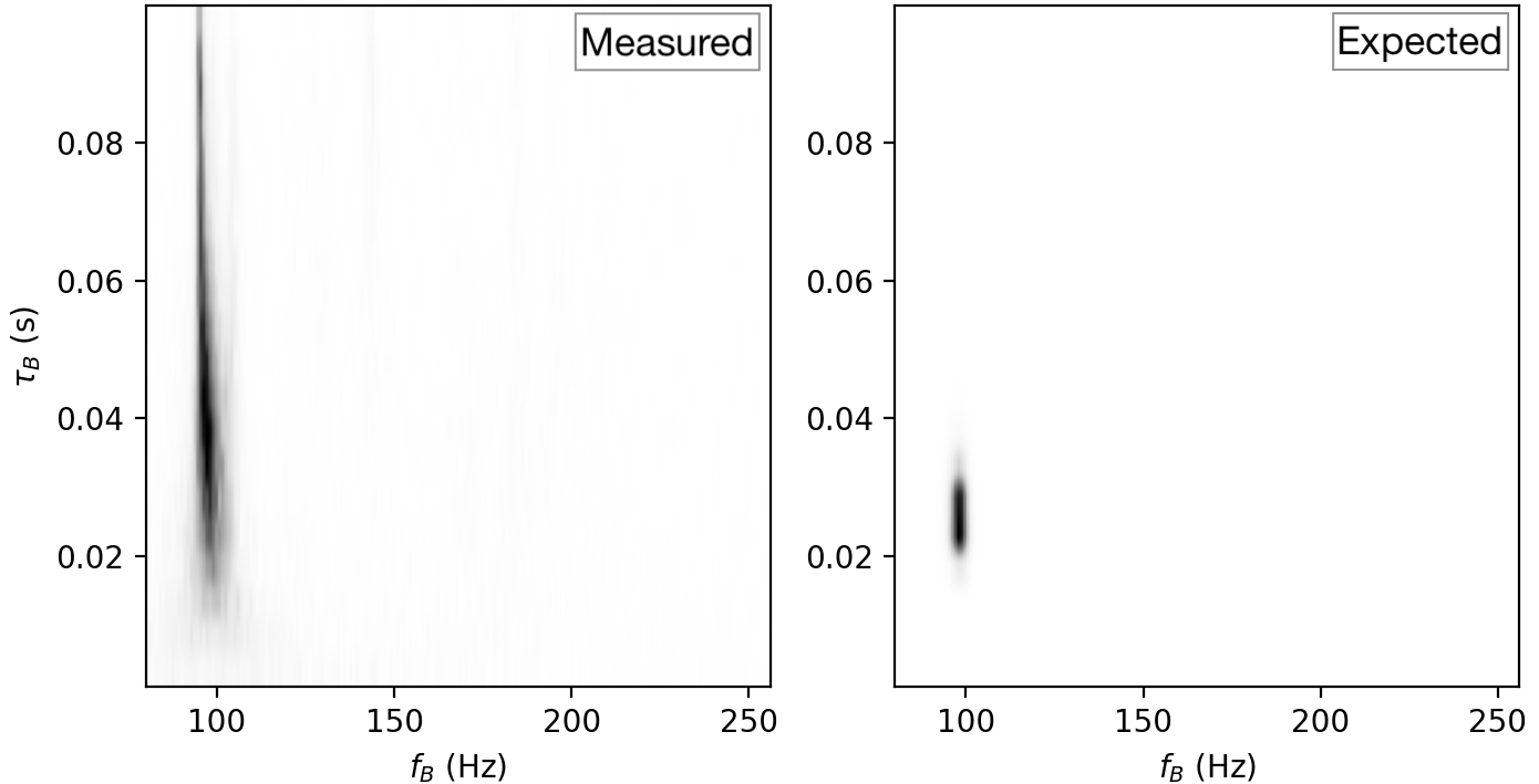
Figure 3: Left: Marginal posterior of the frequency and damping time in frequency range B from the agnostic analysis of GW190521 at $t_{\rm ref}+6\,$ms (same as the heat map in Fig. 1 of Capano et al). Right: the expected distribution of the $(3,3,0)$ mode assuming the mode observed in frequency range A is the dominant, $(2,2,0)$ mode (same as the blue contour in Fig. 1 of Capano et al.) of a Kerr black hole. Darker regions indicate higher probability. The expected distribution is more concentrated due to the larger SNR of the dominant mode. We quantify the agreement between the measured and expected by multiplying the two distributions together and integrating ($\zeta$). The figure and $\zeta$ values are produced using 100 bins each in frequency and damping time.

Two ringdown analyses of GW190521 were presented in Capano et al. Capano et al. (2021): an “agnostic” analysis and a “Kerr” analysis. In the former, the data were analyzed using three QNMs with no assumption made about the relationship between the frequency and damping times of each mode. To prevent all three modes from locking on to the single dominant mode, each mode was assigned a separate frequency range: 50 – 80Hz (range “A”), 80 – 256Hz (range “B”), and 15 – 50Hz (range “C”). Range A covered the dominant mode, which was clearly visible in the data. This analysis was repeated in intervals of 6ms, between $t_{\rm ref}+[0,24]\,$ms.

A signal with a well-defined posterior was found in Range A, having frequency $\sim 63$ Hz and damping time $\sim 26$ ms (see Fig. 1 of Capano et al.). No signal was found in Range C. A second putative mode was found in Range B. This signal was most pronounced at $t_{\rm ref}+6\,$ ms, at which point it has a frequency of $\sim 98$ Hz and damping time $\sim 40$ ms. As shown in Fig.3, these frequencies and damping times were where one would expect the $(3,3,0)$ would be assuming the remnant of GW190521 is a Kerr black hole, with the signal in Range A being the $(2,2,0)$ mode.

Initially, the agnostic analysis was presented as qualitative evidence for the presence of the $(3,3,0)$ mode. Here, we repeat the analysis on our two sets of injections and use them to develop a statistic to quantify the statistical significance of the agnostic result.

If an observable $(3,3,0)$ mode is truly present in the signal, and it is the only observable mode in Range B, then the measured posterior distribution should peak at the same values as the expected distribution. We expect the measured distribution to be more diffuse than the expected distribution. This is because the expected distribution is derived from the observed dominant mode, which is more accurately measured due to its larger SNR. With these considerations in mind, we quantify the agreement between the measured distribution $p_{\rm meas}(f_{B},\tau_{B})$ and the expected distribution $p_{330}(f_{B},\tau_{B})$ using:

$$\zeta\equiv\int p_{\rm meas}(f_{B},\tau_{B})p_{330}(f_{B},\tau_{B})\mathrm{d}f_{B}\mathrm{d}\tau_{B}.$$ (9)

To evaluate this we construct 2D histograms in Range B using 200 bins in frequency and 20 bins in damping time. This is done at each time step; we then maximize $\zeta$ over all the time steps.

We calculate $\zeta$ for the Control injections. Since these injections have no $(3,3,0)$ mode by construction, the resulting $\zeta$ values represent the distribution of false positives. The cumulative distribution of the maximized $\zeta$ is shown by the black line in Fig. 4. We also calculate $\zeta$ for the Signal injections that have post-merger SNR $>$ 4. The cumulative distribution of the maximized $\zeta$ is also shown in Fig. 4 as a blue line. As evident in the figure, we find good separation between the signal and control injections.

Calculating $\zeta$ for GW190521, we find that it is at a maximum at $t_{\rm ref}+6\,$ms, with a value of 1.27. This is consistent with our initial qualitative assessment that the observed mode is most consistent with the expected $(3,3,0)$ mode at $6\,$ms. As shown in Fig. 4, only two of the 500 Control injections have a $\zeta$ larger than GW190521. We therefore conclude that the probability of obtaining a $\zeta$ greater than or equal that of GW190521 by chance from noise is $0.004$.

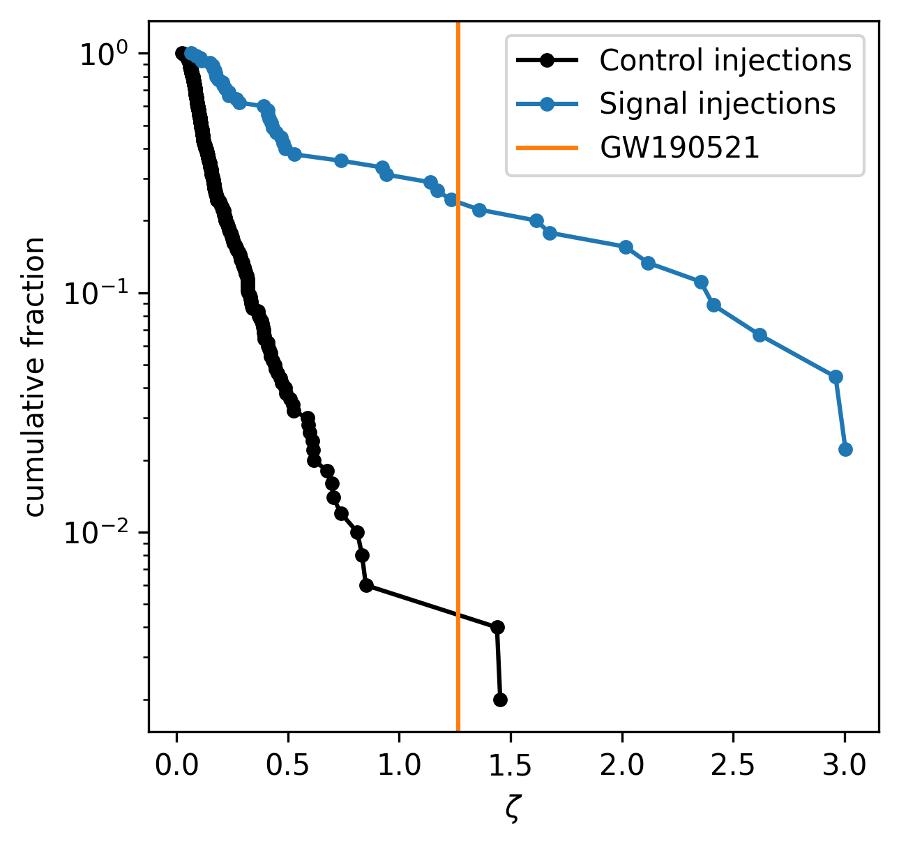
Figure 4: Cumulative distribution of $\zeta$ values for the Control injections (black dots/line) and the Signal injections (blue dots/line). The orange vertical line shows $\zeta$ for GW190521. We use the cumulative distribution of Control injections to estimate a p-value for the $\zeta$ of GW190521. Since two of the 500 Control injections have a $\zeta$ larger than GW190521, we estimate the p-value of the agnostic result to be 0.004

V Statistical significance of the Kerr analysis

In the Kerr analysis we assume the final black hole is described by the Kerr metric. In this case, the frequencies and damping times of all post-merger QNMs are given uniquely by the mass and spin of the black hole. Each additional mode therefore adds two additional degrees of freedom: one for the amplitude and one for the phase of the mode. The relative amplitudes and phases of the modes can in principle be determined by the pre-merger component masses, their spins, and their relative orientation at merger.

Knowing what amplitude and phase to use for each mode requires detailed knowledge of the pre-merger conditions, which are not easily discernible for events like GW190521 in which the pre-merger signal is short and difficult to observe. Furthermore, models mapping pre-merger properties to post-merger quasi-normal modes (QNMs) are limited for highly precessing systems, particularly those with large ($\gtrsim 2$) mass ratios. For these reasons, even when assuming a Kerr model for the post-merger signal, we use uniform priors on the phases and relative amplitudes of the sub-dominant modes with respect to the dominant mode.

Using such broad priors on amplitude and phase makes the analysis susceptible to overfitting. In principle, all modes are present in the signal. However, the vast majority of these modes are negligible compared to the dominant mode. For the types of signals detectable by the current generation of detectors, we expect only a few fundamental modes to have amplitudes that are at most $O(10\%)$ of the dominant mode’s Berti et al. (2016); Cabero et al. (2020). A signal model that contains more than a few modes with such broad priors is effectively unphysical, as it is more likely to fit to noise elements rather than signal (assuming the signal is sufficiently close to GR). To give meaningful results, the signal model should only include the observable modes, not the possible ones.

As with the agnostic analysis, the Kerr analysis also needs to determine when the observable modes are present. Before the merger the QNM model is not valid – there is not a single perturbed black hole at this point. During the merger there may be non-linear components to the signal and/or significant contributions from overtones. Too late after the merger, and the signal will have damped away too much to make anything but the dominant mode observable.

We address both challenges through the use of Bayes factors. Given a signal model with observable modes $\vec{X}=\{(2,2,0),...\}$ at a given time $t-t_{\rm ref}$, we calculate the evidence that the data contain those modes at that time,

$$Z_{\vec{X}}(t)=\int p(\vec{s}|\{\vec{\lambda}_{\vec{X}};t\},h)p(\{\vec{\lambda}_{\vec{X}};t\}|h)\mathrm{d}\vec{\lambda}_{\vec{X}}.$$ (10)

Taking the ratio of this evidence to the evidence for the $(2,2,0)$-only model ($Z_{220}$) at the same time gives the relative odds (or Bayes factor) that the data favor that model as compared to the $(2,2,0)$-only model.

As discussed above, we do not normalize the likelihood function in our analysis. This means that evidence values at different times cannot be directly compared to each other. However, the likelihood function’s normalization factor cancels in the Bayes factor since the normalization only depends on the noise properties and not the signal model. It is therefore possible to compare Bayes factors at different times.

Taking the point that $Z_{\vec{X}}/Z_{220}$ is at a maximum yields the time that the model with modes $\vec{X}$ is the best fit to the data relative to the $(2,2,0)$ model. However, the $(2,2,0)$-only model is known not to be a good model for the signal at merger Giesler et al. (2019). As a result, if we find $Z_{\vec{X}}/Z_{220}$ to be large at some time, it is not clear if this is because modes $\vec{X}$ are a good model for the signal, or if the $(2,2,0)$-only model is just a very bad model at that time. Put another way, $Z_{\vec{X}}/Z_{220}$ only tells us whether the $\vec{X}$ modes are a better fit for the data than just the $(2,2,0)$, not whether the $\vec{X}$-modes are truly observable. This problem becomes particularly acute as we get close to merger.

To account for this, we make use of the observation in Ref. Giesler et al. (2019) that including overtones of the dominant mode better fit the signal close to (or even at) merger than the $(2,2,0)$-mode only. We modify the Bayes factor to be

$$\mathcal{B}(X,t)\equiv\frac{Z_{X}(t)}{\max\{Z_{220},Z_{220+221}\}}$$ (11)

for all models $X\neq(2,2,0)+(2,2,1)$ (for the $(2,2,0)+(2,2,1)$ model we simply use $\mathcal{B}=Z_{220+221}/Z_{220}$). This allows us to both identify the most likely observable modes and the time at which they are most observable.

When applying this method to GW190521 we find $\mathcal{B}$$(220+330)$ to peak at $t_{\rm ref}+6\,\mathrm{ms}$ with a value of $56\pm 1$. This means that the $(2,2,0)+(3,3,0)$ model is $56$ times more likely to be true than the $(2,2,0)$-only model, qualifying it as “strong” evidence. In other words, if the signal did not have an observable $(3,3,0)$ mode, then we should expect to get a $\mathcal{B}$ as large as this from noise only 1 in $56$ times.

To test the validity of this observation, we repeat the Kerr analysis on our Control injections. As with GW190521, we repeat the analysis on a grid of times spanning $t_{\rm ref}+[-9,24]\,$ms, although to reduce computational cost for the large number of analyses involved, we sample in intervals of $3\,$ms instead of the $1\,$ms interval used in Capano et al. Since our Control injections contain no $(3,3,0)$ mode by construction, any large $\mathcal{B}$ observed with them is a false alarm. If our analysis assumptions are correct – that the real data is Gaussian and that we are after the merger – then on average we expect to get a $\mathcal{B}\geq 56$ from $8.9$ of the 500 injections.

Figure 5 (left) shows the cumulative fraction of Control injections that yield Bayes factors larger than the value given on the x-axis. For larger $\mathcal{B}$, we expect the distribution to follow the line $1/x$. We show two results: one in which we maximize $\mathcal{B}$ over all times tested, $t-t_{\rm ref}\in[-9,24]\,$ms and one in which we maximize over times $t-t_{\rm ref}\in[0,24]\,$ms. When maximizing over all times, we find that the injected distribution does not follow the expected distribution of $1/x$; more injections yield large Bayes factors than expected from noise. At the Bayes factor found for GW190521 ($56\pm 1$), 16 of the injections yield larger Bayes factor, whereas we expect $\sim 9$. However, when maximizing over times $t-t_{\rm ref}\geq 0$, the injections show remarkable agreement with the expected distribution. Indeed, we find 10 Control injections yield a $\mathcal{B}\geq{56\pm 1}$.

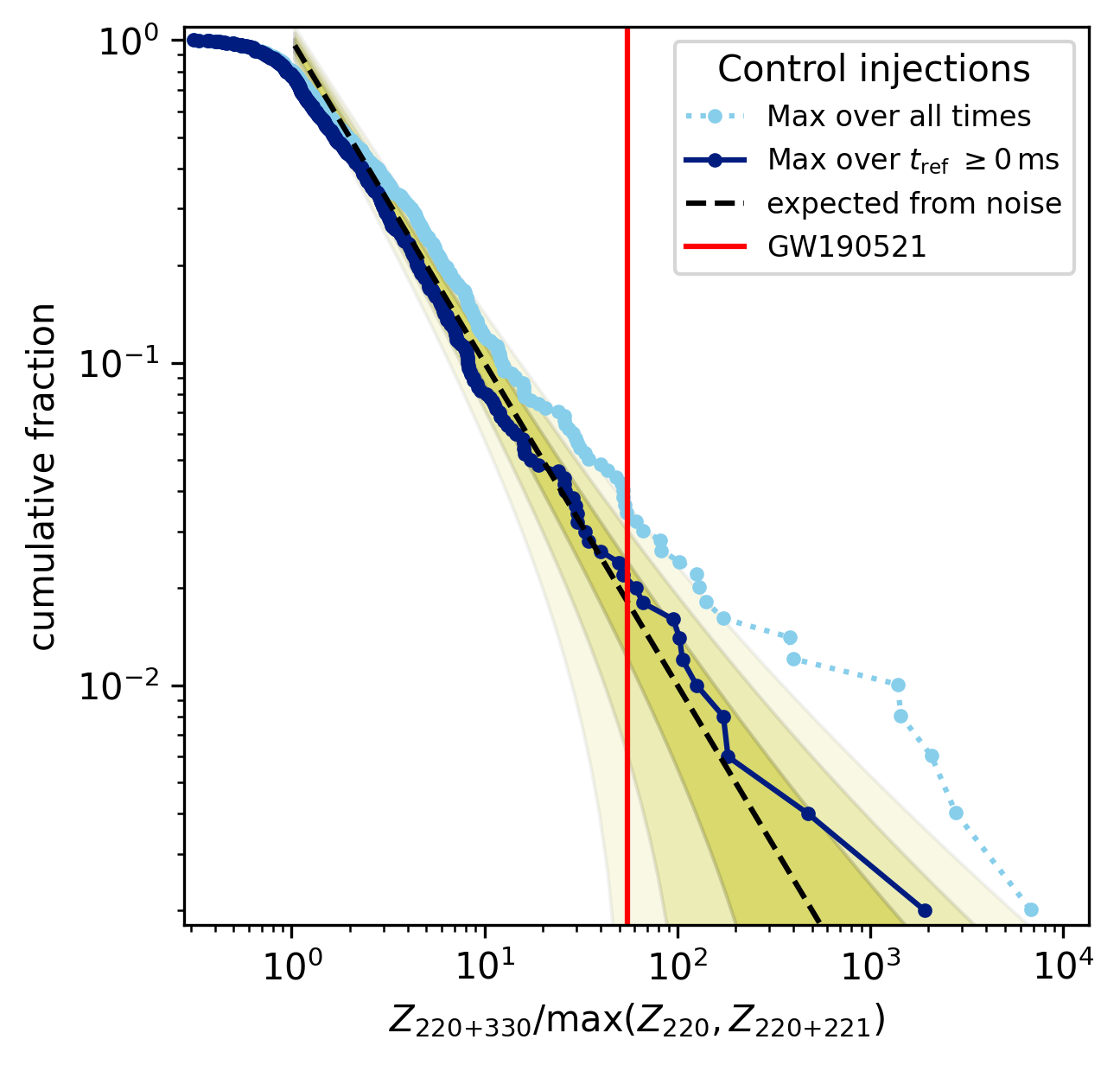
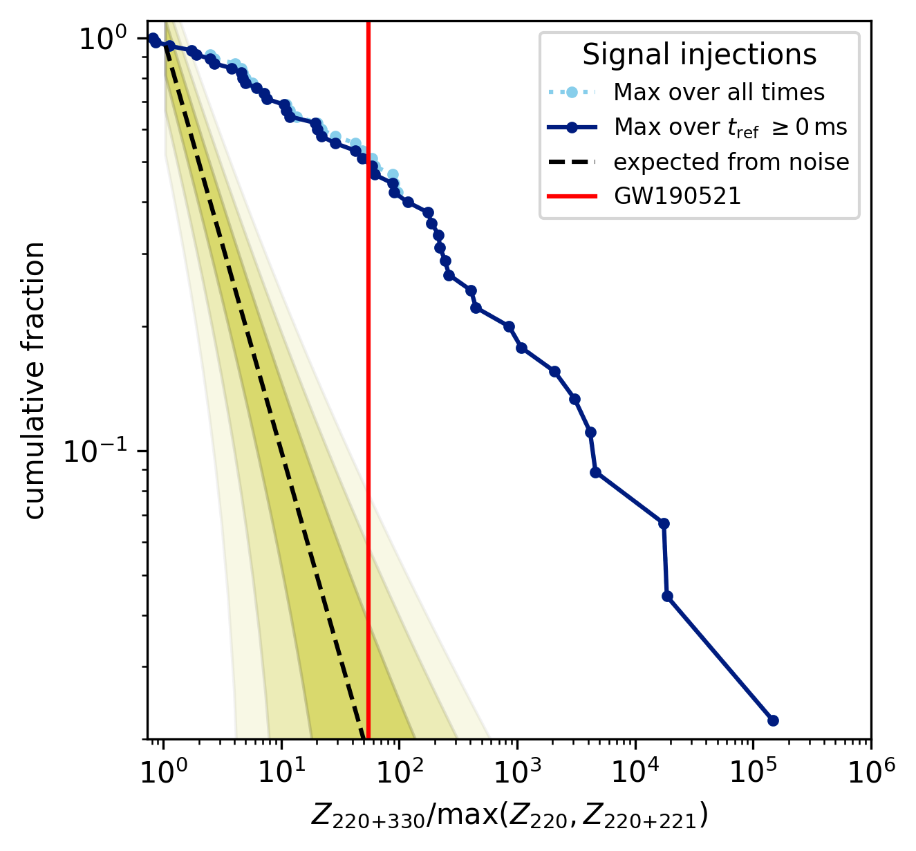
Figure 5: Left: Cumulative fraction of Control injections (i.e., ones without a $(3,3,0)$ mode in the ringdown) versus $(3,3,0)$ Bayes factor maximized over time. Since these injections have no $(3,3,0)$ mode in the ringdown, we expect the cumulative distribution of Bayes factors $\gtrsim 2$ when calculated after the merger to follow the black-dashed line. Shaded yellow regions show the 1-3$\sigma$ deviation regions. The dark blue markers/line show the cumulative distribution of Bayes factors for the Control injections when maximized over time steps $\geq t_{\rm ref}$. For all injections $t\geq t_{\rm ref}$ was after the merger. This line follows the expected distribution. Light blue markers/lines show the distribution of Bayes factors when maximized over all times, including before merger. We get an elevated set of Bayes factors in this case, since the ringdown model is no longer valid before merger. The red vertical line shows the maximized Bayes factor for GW190521 ($56\pm 1$), which occurred at $t_{\rm ref}+6\,$ms. On average, we expect 8.9 out of the 500 injections to have a Bayes factor greater than this; we find 10 when maximized over $t_{\rm ref}\geq 0$. Based on this, we conclude that the quoted Bayes factor for GW190521 is statistically sound. Right: Equivalent plot for Signal injections that have an $\ell,m=(3,3)$ post-merger SNR of at least 4. Contrary to the Control injections, we find the Bayes factors of this set of 45 injections to stay substantially above the noise background. When maximized over $t\geq t_{\rm ref}$, 22 of the 45 injections have a Bayes factor greater than GW190521. This indicates that our pipeline is capable of detecting large Bayes factors when a $(3,3,0)$ mode is present.

Maximizing over all grid times yields an excess of large Bayes factors because the negative times include times before merger for all of the injections (note the distribution of merger times for the NRSurrogate results in Fig. 2). As stated above, before merger the signal is not a superposition of QNMs. This breaks one of our assumptions above. Put another way – anything not modeled by our signal model is “noise”; in the pre-merger regime the “noise” is not Gaussian, and so larger Bayes factors can be obtained than otherwise expected.

However, this only happens if we sample before the merger. By maximizing over $t-t_{\rm ref}\in[0,24]\,$ms we are in the post-merger regime for 174 of the 500 the injections. In this case, we get good agreement with the expectations. We find similarly good agreement if we use our knowledge of the injections’ coalescence time to only maximize over grid points that occur after $t_{c}$. Doing so introduces complications due to the fact that a different number of grid points is maximized over for each injection; see Appendix B for more details.

In order for the larger-than-expected false alarm rate to apply to GW190521, the time at which the maximum Bayes factor occurred ($t_{\rm ref}+6\,\mathrm{ms}$) would have to have been before the merger. Of the 500 Control injections only 15 had coalescence times after $t_{\rm ref}+6\,\mathrm{ms}$. We therefore conclude this scenario to be unlikely, and use the result when maximizing over $t_{\rm ref}\geq 0$. Given the excellent agreement between expectations and measurement, we conclude that our measured $(3,3,0)$ Bayes factor for GW190521 is valid.

To check that our code can recover large Bayes factors when a signal actually has a $(3,3,0)$ mode, we repeat this analysis on the Signal injections. The result is summarized in Fig. 5 (right). As expected, the cumulative distribution of Bayes factors for Signal injections does not follow the distribution expected from noise. We also find there to be little difference between maximizing over $t-t_{\rm ref}\in[-9,24]\,$ms and $t\geq t_{\rm ref}$. Of the 45 Signal injections, 22 have Bayes factors larger than GW190521 when maximized over $t\geq t_{\rm ref}$ while 23 have larger Bayes factors when maximized over all times.

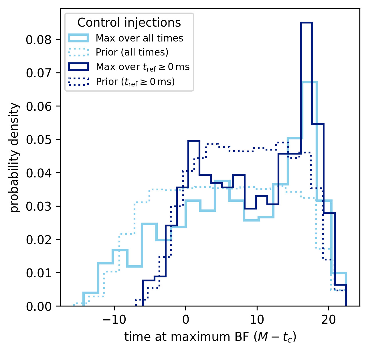
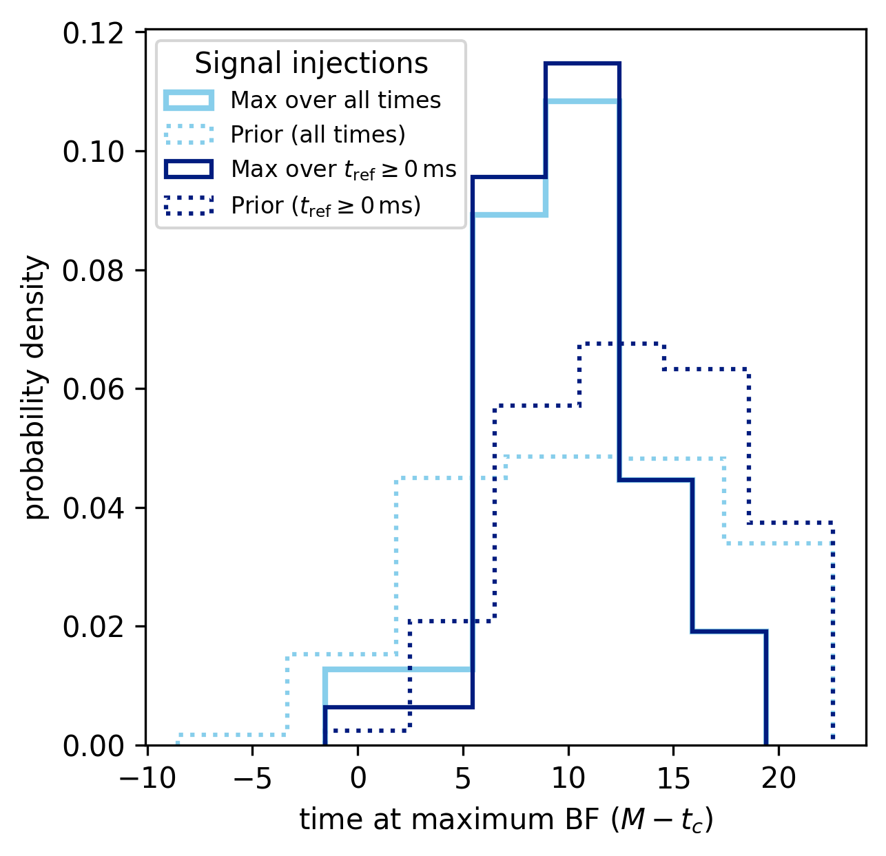
Figure 6: Left: Distribution of times at which the maximum Bayes factor $Z_{220{+}330}/\max\{Z_{220},Z_{220{+}221}\}$ occurred for the Control injections. Times are quoted in units of mass $M$ after $t_{c}$. Shown are when the maximization is done over the entire time period sampled (light blue) and when it is done over just $t_{\rm ref}\geq 0$ (dark blue). The prior is also shown (dotted lines). The distribution is consistent with noise, as it largely uniform with peaks only near the boundaries. These peaks are due to the Bayes factors not being completely independent in time. Right: Equivalent plot for the Signal injections. Here, the Bayes factors tend to peak at $\sim 10M$ after merger. This is consistent with expectations for when a QNM description of the post-merger signal that includes only fundamental modes becomes valid Buonanno et al. (2007); Berti et al. (2007); Kamaretsos et al. (2012).

Figure 6 shows the distribution of times at which the maximum Bayes factor occurs for the Control (left) and Signal (right) injections. In the case of the Control injections, no particular time is favored, as would be expected from noise. There is an excess in the distribution near the boundaries, but this is expected since the Bayes factor is not independent between consecutive time steps. If the Bayes factor is large at a given time, it is more likely to be elevated at surrounding times, due to the autocorrelation length of the template signal. In noise the maximum Bayes factor is therefore more likely to occur close to the boundary.

Conversely, for the Signal injections the distribution in time is peaked at $\sim 10M$ after merger. This is consistent with expectations. Numerical simulations have shown that a QNM description of the signal using only fundamental modes becomes valid between $10$ and $20M$ after merger Buonanno et al. (2007); Berti et al. (2007); Kamaretsos et al. (2012). That the pipeline recovers large Bayes factors when the signal is present and recovers those Bayes factors at $\sim 10M$ after merger validates its ability to recover the $(3,3,0)$ mode from a signal if it is present.

VI Tests of the no-hair theorem

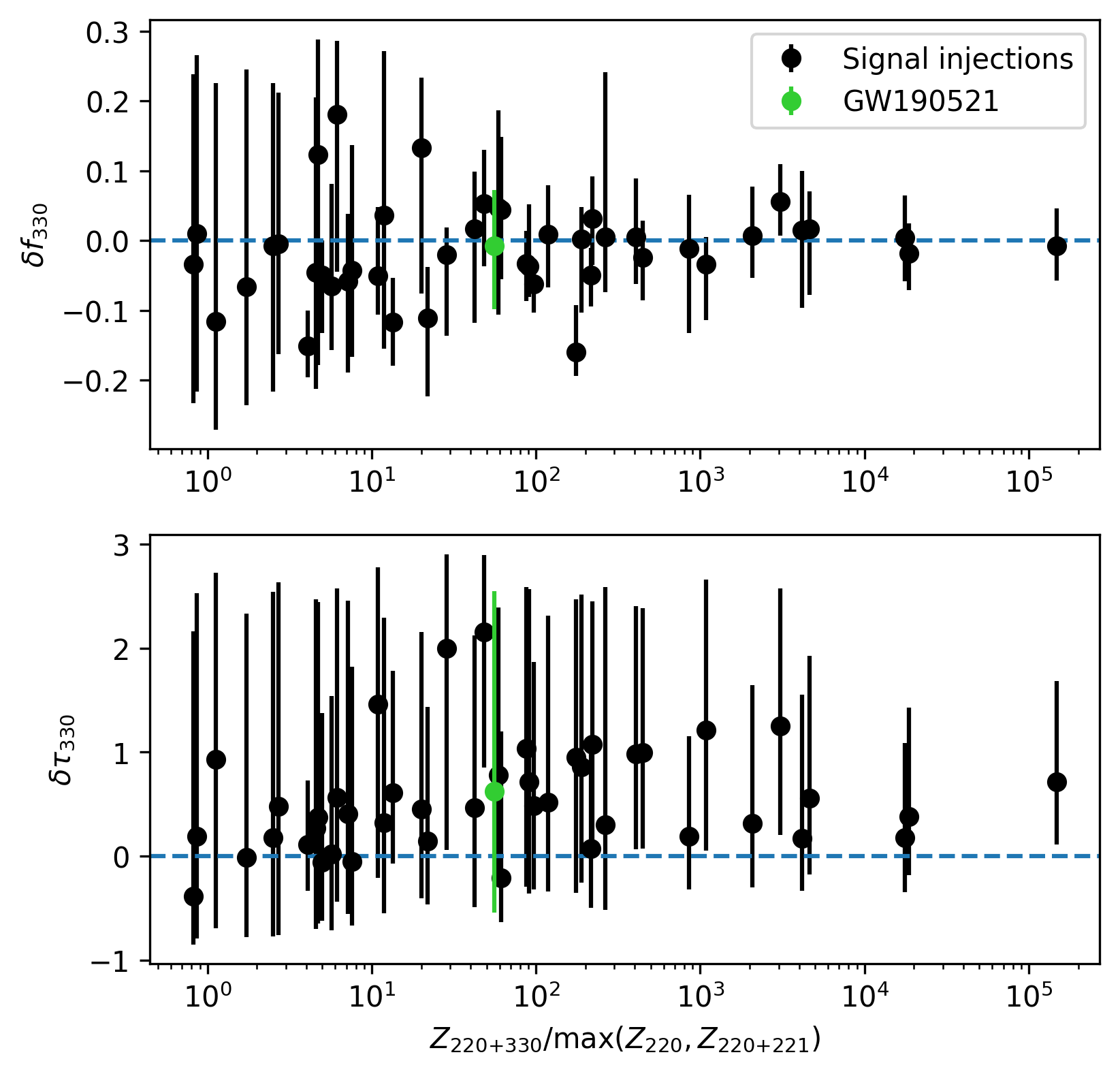
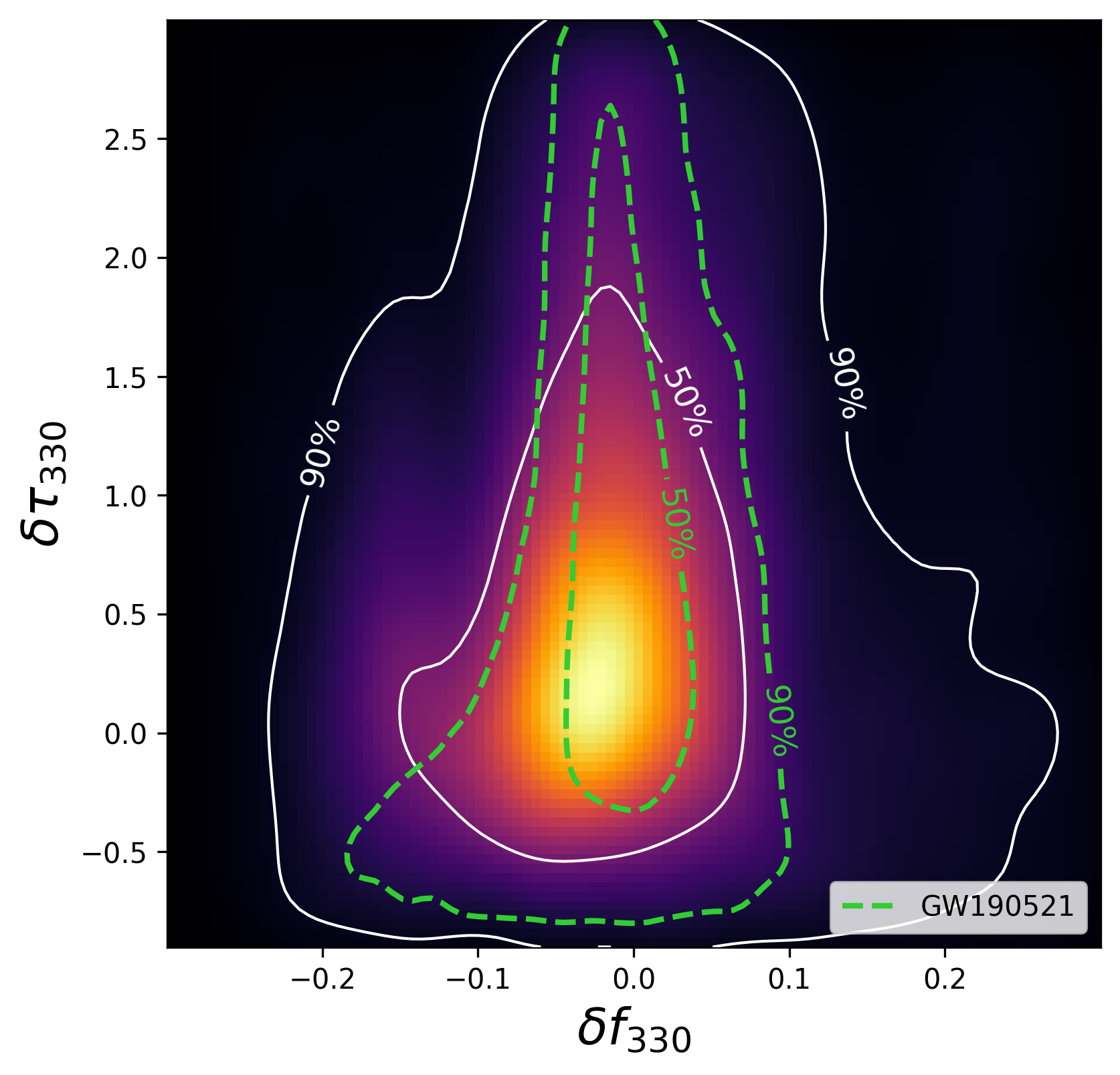
Figure 7: Kerr deviation parameters $\delta f_{330}$ and $\delta\tau_{330}$ evaluated at the time of maximum $(2,2,0){+}(3,3,0)$ Bayes factor of the Signal injections. Left: Marginalized distribution of the parameters as a function of Bayes factor for individual injections. Markers indicate the median value; errorbars show the $90\%$ credible range. For comparison, results from GW190521 are also plotted. Right: The 2D marginal distribution on $\delta f_{330}$ and $\delta\tau_{330}$ averaged over all the injections. This is obtained by adding together all of the injections’ 2D marginal distributions. Dashed green contours show $50\%$ and $90\%$ credible region from GW190521. On average, $\delta f_{330}$ is concentrated close to zero (the expected Kerr value), and it approaches zero as the Bayes factor increases; damping time is not well measured. The constraints obtained on both parameters from GW190521 are consistent with the injections.

With more than one ringdown mode, a non-trivial test of the black hole no-hair theorem can be performed Dreyer et al. (2004). Here we parameterize this test through the deviations $\delta f_{\ell mn}$, $\delta\tau_{\ell mn}$ associated with the measured frequency and damping time of the sub-dominant mode or the overtone.

The deviation parameters are defined by $f_{\ell mn}=(1+\delta f_{\ell mn})f_{\ell mn}(M_{f},\chi_{f})$ and equivalently for $\tau_{\ell mn}$. The mappings $f_{\ell mn}(M_{f},\chi_{f})$ and $\tau_{\ell mn}(M_{f},\chi_{f})$ to the black hole’s final mass and spin $M_{f},\chi_{f}$ assume Kerr and are calculated using the pykerr package Capano (2021). We fix the dominant mode’s frequency and damping time to their Kerr values when doing this test, as has become common Abbott et al. (2020b); Isi and Farr (2021), while varying the final mass and spin. We then have four additional free parameters for each harmonic that is varied in the test, the deviation parameters $\delta f_{\ell mn},\delta\tau_{\ell mn}$, and the mode’s phase $\phi_{\ell mn}$ and amplitude $A_{\ell mn}$.

In Capano et al. we used GW190521 to apply this test to both the $(\ell,m,n)=(3,3,0)$ mode and the $(2,2,1)$ overtone of the dominant mode. Since these modes were best measured at different times, we did not test these modes simultaneously. Instead, the $(2,2,1)$ overtone deviation analysis was done when the Bayes factor for the overtone model was at a maximum, at $t_{\rm ref}-7\,$ms, while the $(3,3,0)$ deviation analysis was done at $t_{\rm ref}+6\,$ms. Since the $(2,2,0)+(2,2,1)$ and $(2,2,0)+(3,3,0)$ models were the most favored models at these respective times, we did not include any other modes when doing these tests. In other words, the intrinsic parameters for the $(3,3,0)$ test were $\{M_{f},\chi_{f},\delta f_{330}\,\delta\tau_{330}\,A_{220},\phi_{220},A_{330}/A_{220},\phi_{330}\}$, and likewise for the $(2,2,1)$ test. See Table 1 for the complete list of parameters and priors used.

The results of these tests on GW190521 yielded excellent constraints on $f_{330}$, with $\delta f_{330}=-1^{+8}_{-9}\,\%$ (90% credible interval). The damping time was only weakly constrained, with $\delta\tau_{330}=60^{+190}_{-120}\,\%$. Previously, sub-$20\%$ constraints on any sub-dominant fundamental mode were not expected until at least the next generation of detectors Berti et al. (2016); Cabero et al. (2020). This is because observations of binary black hole mergers prior to GW190521 had smaller total masses and were primarily equal mass ratio. The constraint on $f_{330}$ was also substantially better than has been obtained on the $(2,2,1)$ overtone with other events. The best single-event constraint on $\delta f_{221}$ as reported by the LVC was $\sim\pm 50\%$ Abbott et al. (2021c). Combining results over 21 observations yielded $\delta f_{221}=1^{+27}_{-28}\%$ Abbott et al. (2021d), still a factor of $\sim 3$ larger than the constraint on $\delta f_{330}$ obtained from GW190521 alone.

Here, we repeat our no-hair test on the Signal injections to check whether the constraints we obtained on the $(3,3,0)$ mode are reasonable at the signal strength of GW190521. Since the simulations satisfy general relativity the results from these tests indicate what constraints can be obtained given the type of signal observed and the quality of the data around that time. For this test we use 44 of the Signal injections, generated with IMRPhenomTPHM including all its available modes. Each injection is analyzed at its time of maximum $(2,2,0)+(3,3,0)$ Bayes factor. This replicates what was done with GW190521 in Capano et al.

Results for $\delta f_{330}$ and $\delta\tau_{330}$ using the Signal injection set are summarized in Fig. 7. Shown are 1D marginal results for each injection. We also show the 2D marginal distribution on these parameters, averaged over all the injections. Results from GW190521 are also plotted for comparison. On average, the injections’ $(3,3,0)$ deviation parameters $\delta f_{330}$ and $\delta\tau_{330}$ are centered near zero, and $f_{330}$ becomes better constrained as the Bayes factor increases. The constraints derived from GW190521 are consistent with these results. This indicates that at the signal strength of GW190521, a constraint on $\delta f_{330}\sim 10\%$ is reasonable for GR signals even though only two QNM modes are included in the model at the time of the analysis.

We also perform the same analysis on the $(2,2,1)$ overtone at, or just after, the coalescence time of the Control injections. Doing so, we find that the posterior on $\delta f_{221}$ and $\delta\tau_{221}$ are peaked away from zero on average; see Appendix C for details. These results are consistent with the overtone deviations we observed in GW190521 Capano et al. (2021). Since the injections satisfy general relativity, this indicates that the deviations observed in GW190521 are not due to violations to GR. The $(2,2,0){+}(2,2,1)$ model is not a sufficiently complete description of the signal at merger.

Note that the $(2,2,0){+}(3,3,0)$ model is not a complete description of the signal either, even at $10\,M$ after merger. Other modes are present in these signals; as the SNR of signals increases it will be necessary to include additional modes in the model. However, our results indicate that at the signal strength of GW190521, the $(2,2,0){+}(3,3,0)$ model is sufficient to describe the signal and to constrain the deviations on the $(3,3,0)$ mode at the $\sim 10\%$ level, as we obtained with GW190521.

VII Conclusions

The Bayes factor for two Kerr ringdown modes over just one mode was estimated to be ${56\pm 1}$ for GW190521 in Capano et al. Capano et al. (2021) Here, we find that of 500 simulated signals with higher ringdown modes explicitly turned off, only 10 are recovered with a Bayes factor higher than 56. Thus a statistic at least as significant as GW190521 occurs once in 50 times. We have in addition demonstrated that the analysis can detect a $(3,3,0)$ mode when it is present in the data.

We also developed a statistic $\zeta$ to quantify the agnostic analysis. This involves comparing the consistency of the two-dimensional frequency and damping-time posterior of the second mode with that predicted by the frequency and damping-time posterior from the first mode, assuming that they are the $(2,2,0)$ and $(3,3,0)$ modes of a Kerr black hole. We showed that this statistic was able to separate simulations with an observable $(3,3,0)$ mode from those without. Applying this to GW190521, we find that the probability of getting a $\zeta$ as large as that of GW190521 by chance from simulations that do not have a $(3,3,0)$ mode is $0.004$.

Our results for the no-hair theorem test in Sec. VI show that the constraints on the $(3,3,0)$ mode observed for GW190521 in Capano et al. are consistent with what is obtained using simulated GR signals. Conversely, we find that the posterior on $(2,2,1)$ deviations are peaked away from the expected Kerr result when GR waveforms are analyzed, just as it was for GW190521. The poor constraints obtained on the $(2,2,1)$ overtone indicate the $(2,2,0){+}(2,2,1)$ QNM model is not a complete description of the signal at merger, at least not for GW190521-like signals. This does not mean a QNM model is completely invalid at merger. Indeed, our $(2,2,0){+}(3,3,0)$ results depend on using the $(2,2,0){+}(2,2,1)$ model to identify times close to merger and obtain Bayes factors that match statistical expectations. The $(2,2,0){+}(2,2,1)$ model is therefore a useful model even if it is not a complete one.

It may also be possible to use a QNM model at merger to constrain deviations from GR if enough overtones are included in the model. Determining the appropriate number of observable overtones without overfitting the data is a delicate question, however, beyond the scope of this study. Our results here indicate that performing the no-hair test on fundamental modes, later in the signal, largely sidesteps such questions (at least at currently observable SNR), yielding much tighter and more reliable constraints.

Our simulation campaign supports the conclusion that the $(3,3,0)$ quasi-normal mode is observable in the ringdown of GW190521, and that this mode is consistent with general relativity.

Appendix A Effect of polarization marginalization on the Bayes factor

In the initial analysis in Capano et al. Capano et al. (2021) we used dynesty to sample over all parameters for the Kerr analysis listed in Table 1. We found a maximum Bayes factor of $44^{+6}_{-5}$ in favor of the $(2,2,0)+(3,3,0)$ model at $t_{\rm ref}+7\,$ms. However, this method proved time-consuming as the sampler struggled to converge for some mode combinations. The difficulty largely arises from the combination of the phases of the modes and the polarization angle. In particular, for GW190521 the phase of the dominant mode and the polarization are degenerate, as the polarization is not measured well due to the low SNR in the Virgo detector. This results in a banding pattern in the marginal likelihood between these parameters that is a challenge to sample.

Sampling over all parameters would have been unfeasible for the large number of injections we analyzed here. We therefore introduced a modified gating-and-in-painting model that numerically marginalized over the polarization using 1000 grid points. This marginalization technique was employed in the 3-OGC Nitz et al. (2021c) and 4-OGC analyses Nitz et al. (2021a), where it was found to speed convergence for full IMR templates with sub-dominant modes. We are able to apply the same technique here because the dependence on the polarization is approximately constant over time for a short-duration event like GW190521, and so can be separated from the gating-and-in-painting procedure.

In implementing the polarization marginalization, we discovered that we obtained a larger Bayes factor for GW190521 one ms earlier, at $t_{\rm ref}+6\,$ms. To verify this, we repeated the $+6\,$ms and $+7\,$ms analysis 10 times using different starting seeds. We also repeated each analysis once with double the number of live points. We found consistently larger values at $+6\,$ms. Averaging the Bayes factors over the runs we obtained $56\pm 1$ at $+6\,$ms and $45\pm 1$ at $+7\,$ms, where the uncertainty is reported with 1$\sigma$. We further verified these Bayes factors by using the Savage-Dickey ratio on the $(3,3,0)$ amplitude posterior to estimate the Bayes factor, and obtained similar results as reported by dynesty’s estimate.

The result at $7\,$ms was consistent with our initial result in Capano et al., but the result at $6\,$ms was substantially higher. Our initial estimate for the Bayes factor at $+6\,$ms (without marginalization) was $40^{+5}_{-4}$. Evidently, without marginalization, the sampler had not fully converged at $6\,$ms, yielding an underestimate of the Bayes factor. Marginalization also affected our $(2,2,1)$ results: we found the Bayes factor for the $(2,2,1)$ mode peaked slightly earlier, at $t_{\rm ref}-7\,$ms instead of the $t_{\rm ref}-5\,$ms that we initially estimated.

Given the robustness of the new results under polarization marginalization, we quote the updated Bayes factor at $t_{\rm ref}+6\,$ms here for GW190521. We also updated Capano et al. to reflect these changes.

Appendix B Maximizing the Kerr Bayes factor after merger

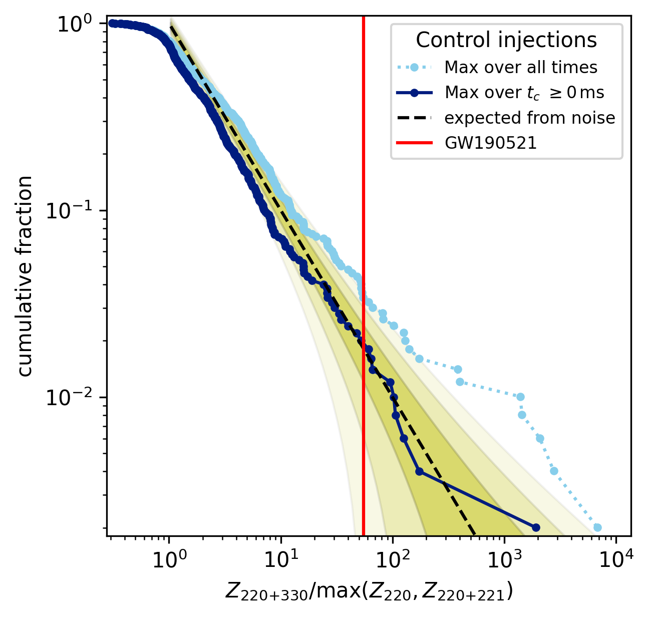
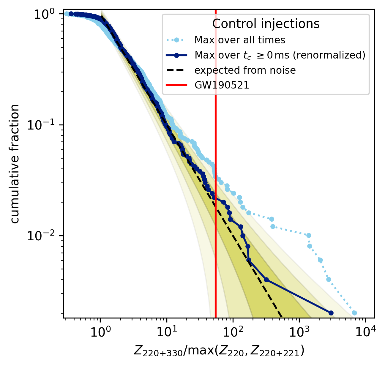
Figure 8: Left: Same as Fig. 5 (left), but with the maximization interval based on the injections’ coalescence time $t_{c}$ (dark blue line). We find excellent agreement with the expected background distribution at large Bayes factors, but a $\sim 3\sigma$ downward deviation in the measured distribution at Bayes factors $\lesssim 20$. This deviation is due to the different maximization range for each injection. Right: Renormalized version of the left plot. Here, we’ve accounted for variations in maximization interval across the Control injections by multiplying their Bayes factor by $(\max N_{\rm grid})/N_{\rm grid}$, where $N_{\rm grid}$ is the number of time points maximized over. We find good agreement with the expected background at both large and small Bayes factors in this case.

As discussed in Sec. V, we obtain good agreement between the expected distribution of Bayes factors and the measured distribution if we restrict the maximization interval to be strictly after the Control injections’ coalescence time $t_{c}$. The result is shown in the left plot of Fig. 8. Above Bayes factors of $\sim 20$ we find excellent agreement with the background. Indeed, we find that 9 of the 500 injections have a Bayes factor larger than GW190521, exactly the amount expected by chance.

However, for Bayes factors $\lesssim 20$ there is a nearly $3\sigma$ downward deviation in the measured background. This deviation is due to the fact that differing numbers of grid points are maximized over when using the injection’s coalescence time. For example, the maximization interval spans nine grid points (spanning $t_{\rm ref}+[0,24]\,$ms) for injections that have a $t_{c}\approx t_{\rm ref}$, whereas the interval is only two grid points for injections with $t_{c}\approx t_{\rm ref}+21$ ms. Although grid points are not independent of each other – if a large Bayes factor exists at a particular point in time, there is a higher probability that its neighbors will also have larger Bayes factors – they are not entirely dependent either. Due to the stochastic nature of the noise, there are random fluctuations in Bayes factors across time. Consequently, if a maximization interval covers fewer grid points, there are fewer opportunities to obtain larger Bayes factors.

Large Bayes factors are not strongly affected by differences in maximization interval, since there is a low probability that a noise fluctuation could produce a larger Bayes factor. This is evident in the left plot of Fig. 8. Conversely, smaller Bayes factors will be affected by this, hence the deviation at lower Bayes factors in that plot.

This issue can be corrected for by multiplying the Bayes factors of each injection by $(\max N_{\rm grid})/N_{\rm grid}$, where $N_{\rm grid}$ is the number of grid points maximized over for the given injection and $\max N_{\rm grid}$ is the largest number of grid points maximized over in the set. Renormalizing the Bayes factors yields the result shown in the right plot of Fig. 8. Now we find good agreement with the expected background and measured distribution at all Bayes factors. With this we find 10 Control injections to have a larger Bayes factor when we expect 9.

Note that the normalization factor implicitly assumes that each grid point is independent of the others. As stated above, this is not the case. Since using this factor tends to overestimate the contribution, this is a conservative error.

Due to these complications we present in the main text the simpler maximization over $t_{\rm ref}\geq 0$.

Appendix C No-hair test of the (2,2,1) mode at merger

The constraints obtained on $\delta f_{221}$ and $\delta\tau_{221}$ using GW190521 were $-0.10^{+0.34}_{-0.05}$ and $0.5^{+0.3}_{-0.7}$, significantly worse than the $(3,3,0)$ constraints. Moreover, the posterior was strongly centered away from the Kerr value of $\delta f_{221}=\delta\tau_{221}=0$, and peaked at the prior boundaries — indicating that had the prior been wider, the maximum posterior density would have been further from the Kerr value. This is despite larger signal-to-noise ratio and significantly larger Bayes factor for the $(2,2,0){+}(2,2,1)$ model as compared to the $(2,2,0){+}(3,3,0)$ model at their respective analyzed times. Three possibilities can explain these results: either the signal significantly violates general relativity, there was significant non-Gaussian noise overlapping the signal, or the $(2,2,0){+}(2,2,1)$ QNM model is not a complete description of the signal at the time analyzed of $t_{\rm ref}-7\,$ms. To disambiguate these scenarios, we also did the no-hair test on the $(2,2,1)$ overtone using our set of Control simulations.

We use the Control injections for the $(2,2,1)$ analysis. As in the agnostic and Kerr studies in the main text, these are generated using the NRSur7dq4 approximant, and include only the $\ell=2$ modes. Instead of using the Bayes factor to determine when to perform the no-hair test (as was done with the real signal), we do the test at the grid point that is closest to, but not before, the coalescence time $t_{c}$. This means that the analyzed times are anywhere from $0$ to $3\,$ms after $t_{c}$ (see Sec. V for details on the timing grid used). The no-hair overtone analysis therefore differs from the real GW190521 analysis, since the real signal will have all modes present (albeit not all observable) and the coalescence time is uncertain. Our motivation in these choices is to make the setup as amenable to constraining the $(2,2,1)$ overtone as possible; i.e., we remove the question as to whether the $(2,2,0)+(2,2,1)$ Bayes factor truly peaks at the merger, and we try to reduce complications arising from additional sub-dominant modes. Due to the large number of Control injections, we draw at random 40 simulations for this analysis.

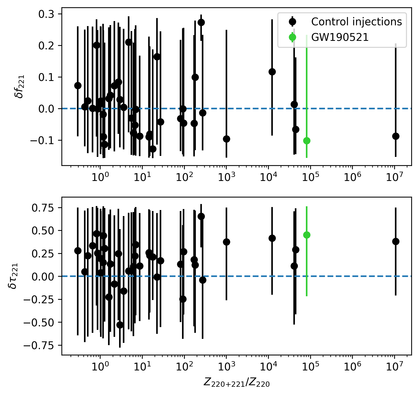
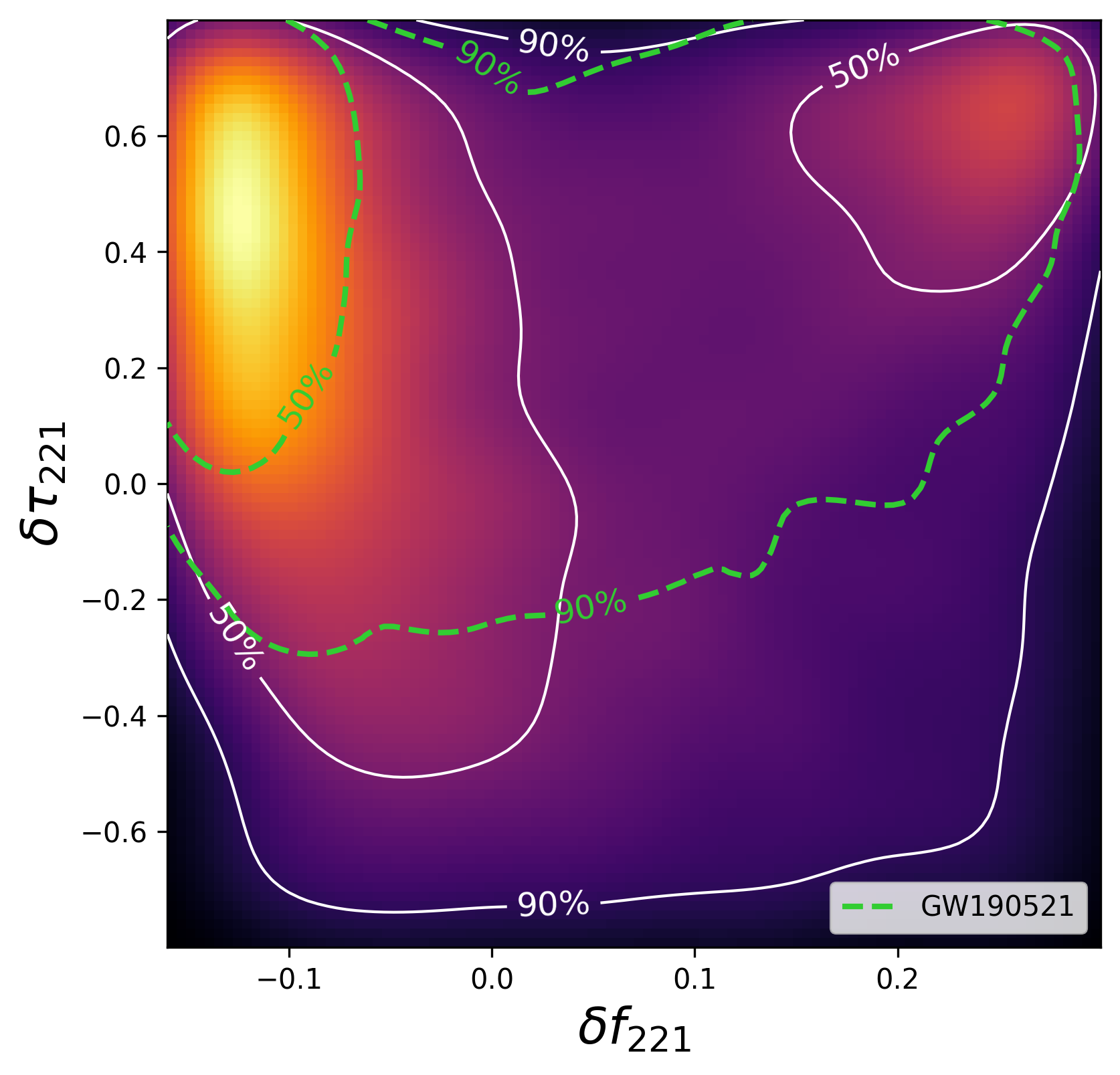
Figure 9: Same as Fig. 7, but for $\delta f_{221}$ and $\delta\tau_{221}$ using a random selection of 40 Control injections. Here, injections are analyzed at or just after $t_{c}$. Results from GW190521 Capano et al. (2021) are also plotted for comparison. Note that the Bayes factor plotted for GW190521 in left panel is the maximum over all time ranges. This may not be at GW190521’s $t_{c}$. Unlike the $(3,3,0)$ results, the $(2,2,1)$ deviation parameters are generally concentrated away from the Kerr value and do not improve with increasing Bayes factor. The results from the injections are consistent with the $(2,2,1)$ deviations observed with GW190521. Since the injections satisfy general relativity and are analyzed at $t_{c}$, the deviations indicate that the $(2,2,0){+}(2,2,1)$ QNM model is not a sufficiently complete description of the signals at $t_{c}$.

Results for $\delta f_{221}$ and $\delta\tau_{221}$ using the Control injection set are summarized in Fig. 9. In contrast to the $(3,3,0)$ mode, the overtone deviation parameters are not centered on zero. Instead, $\delta f_{221}$ displays a bimodal distribution on average, with the data favoring either the largest or smallest deviation as allowed by the prior. The damping time deviation $\delta\tau_{330}$ is also peaked toward large positive values. Neither parameter becomes better constrained with increasing Bayes factor.

The measured deviations on the Control injections’ $(2,2,1)$ overtone are consistent with what was observed in GW190521 (note the comparison in Fig. 9). Since the injections are derived from solutions to General Relativity, the deviations observed in the injections cannot be due to a violation of GR. It is also unlikely that non-Gaussian noise is causing the deviations due to the injections being distributed in time. This suggests that the cause of the deviations is the $(2,2,0){+}(2,2,1)$ model is not a complete description of the signal at $t_{c}$.

This is not altogether surprising; indeed, we do not expect the $(2,2,0){+}(2,2,1)$ model to be complete. Many of the Control injections are highly precessing. Precession causes spherical harmonics with the same $\ell$, but different $m$, to mix together when transforming from the binary’s co-precessing frame to that of an inertial observer far from the binary Varma et al. (2019). his means that even if a waveform with only the $\ell=m=2$ mode is generated in the observer frame, it will contain contributions from the $m\neq 2$ modes in the co-precessing frame. We also found that precession caused the injections’ $(2,-2)$ mode to peak several $M$ after the $(2,2)$ mode. This is different from aligned-spin waveforms, in which there is no mode mixing, and the $-m$ mode is related to the $+m$ mode via $h_{(}\ell-m)=(-1)^{\ell}h^{*}_{\ell m}$.

It seems plausible that the deviations observed in the $(2,2,1)$ overtone are due to the combined effect of mode mixing and asymmetric $-m$ modes, which does not exist in aligned-spin signals like GW150914. To test if this is the case, we performed an analysis in which we shut off all possible mode mixing. This was accomplished by turning off all modes except the $(2,2)$ spherical harmonic in the co-precessing frame prior to transforming to the observer frame. In addition, we generated the $(2,-2)$ spherical harmonic by assuming $h_{\ell-m}=(-1)^{\ell}h^{*}_{\ell m}$. These modifications were accomplished by using the GWSurrogate package Field et al. (2014) to generate the waveforms.

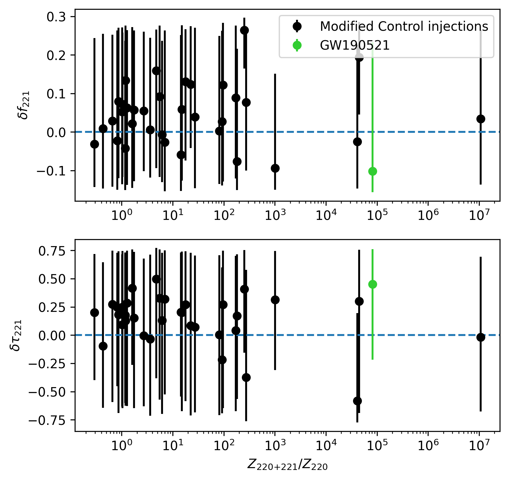
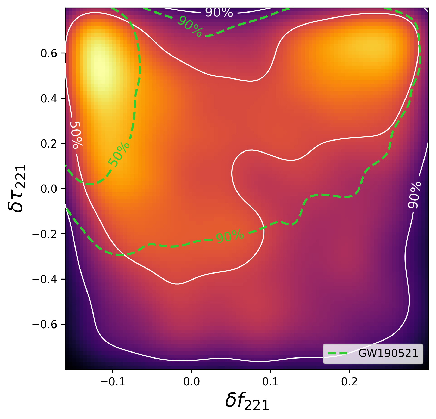
Figure 10: Same as Fig. 9, but using modified Control injections in which all mode mixing due to precession is turned off, and the $(2,-2)$ mode is constructed from the $(2,2)$ mode (see text for details). Plotted are 34 of the 40 injections that were used in Fig. 9; the sampler did not converge for the remaining six injections. Results from GW190521 Capano et al. (2021) are also plotted for comparison. The Bayes factors that give the x-axis in the left figure are taken from the original, unmodified Control injections. The results are similar to the unmodified injections, indicating that the measured deviations in the $(2,2,1)$ overtone are not simply due to mode mixing.

We repeated the $(2,2,1)$ deviation analysis using these modified injections. The combined posterior on $\delta f_{221}$ and $\delta\tau_{221}$ is shown in Fig. 10. There is little difference in the results from the original injection set. On average, $(2,2,1)$ parameters still peak away from zero. This suggests that the measured deviations are not solely due to mode mixing.

Another possibility is that we have not included enough overtones in our signal model. In Giesler et al. Giesler et al. (2019) it was shown that multiple overtones are needed to fully describe the signal at merger. Here, we only included a single overtone because the Bayesian evidence did not favor more than a single overtone in the original GW190521 analysis Capano et al. (2021). Adding additional overtones may fix the deviation, although doing so raises questions of overfitting the data Baibhav et al. (2023). It is also not clear why a single overtone is sufficient for the analysis of GW150914-like signals Giesler et al. (2019), but not GW190521-like signals. A more comprehensive study similar to Giesler et al. but applied to a wider range of mass ratios and spin orientations is warranted; such a study is beyond the scope of this paper.

Regardless of the cause, our results indicate that the $(2,2,0){+}(2,2,1)$ model is simply not a complete description of these simulations at merger, even though it is the most favored QNM model (of the ones we tried) at that time. This is in stark contrast to the $(2,2,0){+}(3,3,0)$ model. As shown in Sec. VI, at the time that the $(2,2,0){+}(3,3,0)$ model is most favored (which, according to Fig. 6 is likely to be $\sim 10\,M$ after merger) we do not find significant deviations in the $(3,3,0)$ mode. This implies that a linear, QNM description of the signal is not sufficient at merger, but is sufficient when the $(2,2,0){+}(3,3,0)$ Bayes factor peaks.

References

- Andersson et al. (2019) L. Andersson, T. Bäckdahl, P. Blue, and S. Ma, (2019), arXiv:1903.03859 [math.AP] .
- Whiting (1989) B. F. Whiting, J. Math. Phys. 30, 1301 (1989).
- Berti et al. (2009) E. Berti, V. Cardoso, and A. O. Starinets, Class. Quant. Grav. 26, 163001 (2009), arXiv:0905.2975 [gr-qc] .
- Dreyer et al. (2004) O. Dreyer, B. J. Kelly, B. Krishnan, L. S. Finn, D. Garrison, and R. Lopez-Aleman, Class. Quant. Grav. 21, 787 (2004), arXiv:gr-qc/0309007 .
- Kamaretsos et al. (2012) I. Kamaretsos, M. Hannam, S. Husa, and B. S. Sathyaprakash, Phys. Rev. D 85, 024018 (2012), arXiv:1107.0854 [gr-qc] .
- Vishveshwara (1970a) C. V. Vishveshwara, Nature 227, 936 (1970a).
- Vishveshwara (1970b) C. V. Vishveshwara, Phys. Rev. D 1, 2870 (1970b).
- Chandrasekhar and Detweiler (1975) S. Chandrasekhar and S. L. Detweiler, Proc. Roy. Soc. Lond. A 344, 441 (1975).
- Thrane et al. (2017) E. Thrane, P. D. Lasky, and Y. Levin, Phys. Rev. D 96, 102004 (2017), arXiv:1706.05152 [gr-qc] .
- Bhagwat et al. (2018) S. Bhagwat, M. Okounkova, S. W. Ballmer, D. A. Brown, M. Giesler, M. A. Scheel, and S. A. Teukolsky, Phys. Rev. D 97, 104065 (2018), arXiv:1711.00926 [gr-qc] .
- Okounkova (2020) M. Okounkova, (2020), arXiv:2004.00671 [gr-qc] .
- Mitman et al. (2022) K. Mitman et al., (2022), arXiv:2208.07380 [gr-qc] .
- Lagos and Hui (2022) M. Lagos and L. Hui, (2022), arXiv:2208.07379 [gr-qc] .
- Cheung et al. (2022) M. H.-Y. Cheung et al., (2022), arXiv:2208.07374 [gr-qc] .
- Jaramillo et al. (2012a) J. L. Jaramillo, R. P. Macedo, P. Moesta, and L. Rezzolla, AIP Conf. Proc. 1458, 158 (2012a), arXiv:1205.3902 [gr-qc] .
- Jaramillo et al. (2012b) J. L. Jaramillo, R. Panosso Macedo, P. Moesta, and L. Rezzolla, Phys. Rev. D 85, 084030 (2012b), arXiv:1108.0060 [gr-qc] .
- Prasad et al. (2020) V. Prasad, A. Gupta, S. Bose, B. Krishnan, and E. Schnetter, Phys. Rev. Lett. 125, 121101 (2020), arXiv:2003.06215 [gr-qc] .
- Mourier et al. (2021) P. Mourier, X. Jiménez Forteza, D. Pook-Kolb, B. Krishnan, and E. Schnetter, Phys. Rev. D 103, 044054 (2021), arXiv:2010.15186 [gr-qc] .
- Forteza and Mourier (2021) X. J. Forteza and P. Mourier, Phys. Rev. D 104, 124072 (2021), arXiv:2107.11829 [gr-qc] .
- Pook-Kolb et al. (2020) D. Pook-Kolb, O. Birnholtz, J. L. Jaramillo, B. Krishnan, and E. Schnetter, (2020), arXiv:2006.03940 [gr-qc] .
- Gupta et al. (2018) A. Gupta, B. Krishnan, A. Nielsen, and E. Schnetter, Phys. Rev. D 97, 084028 (2018), arXiv:1801.07048 [gr-qc] .
- Chen et al. (2022) Y. Chen et al., (2022), arXiv:2208.02965 [gr-qc] .
- Berti et al. (2016) E. Berti, A. Sesana, E. Barausse, V. Cardoso, and K. Belczynski, Phys. Rev. Lett. 117, 101102 (2016), arXiv:1605.09286 [gr-qc] .
- Cabero et al. (2020) M. Cabero, J. Westerweck, C. D. Capano, S. Kumar, A. B. Nielsen, and B. Krishnan, Phys. Rev. D 101, 064044 (2020), arXiv:1911.01361 [gr-qc] .
- Borhanian et al. (2020) S. Borhanian, K. G. Arun, H. P. Pfeiffer, and B. S. Sathyaprakash, Class. Quant. Grav. 37, 065006 (2020), arXiv:1901.08516 [gr-qc] .
- Isi et al. (2019) M. Isi, M. Giesler, W. M. Farr, M. A. Scheel, and S. A. Teukolsky, Phys. Rev. Lett. 123, 111102 (2019), arXiv:1905.00869 [gr-qc] .
- Giesler et al. (2019) M. Giesler, M. Isi, M. A. Scheel, and S. Teukolsky, Phys. Rev. X 9, 041060 (2019), arXiv:1903.08284 [gr-qc] .
- Cotesta et al. (2022) R. Cotesta, G. Carullo, E. Berti, and V. Cardoso, Phys. Rev. Lett. 129, 111102 (2022), arXiv:2201.00822 [gr-qc] .
- Isi and Farr (2022) M. Isi and W. M. Farr, (2022), arXiv:2202.02941 [gr-qc] .
- Nollert (1996) H.-P. Nollert, Phys. Rev. D 53, 4397 (1996), arXiv:gr-qc/9602032 .
- Nollert and Price (1999) H.-P. Nollert and R. H. Price, J. Math. Phys. 40, 980 (1999), arXiv:gr-qc/9810074 .
- Jaramillo et al. (2021) J. L. Jaramillo, R. Panosso Macedo, and L. Al Sheikh, Phys. Rev. X 11, 031003 (2021), arXiv:2004.06434 [gr-qc] .
- Jaramillo et al. (2022) J. L. Jaramillo, R. Panosso Macedo, and L. A. Sheikh, Phys. Rev. Lett. 128, 211102 (2022), arXiv:2105.03451 [gr-qc] .
- Destounis et al. (2021) K. Destounis, R. P. Macedo, E. Berti, V. Cardoso, and J. L. Jaramillo, Phys. Rev. D 104, 084091 (2021), arXiv:2107.09673 [gr-qc] .
- Capano et al. (2021) C. D. Capano, M. Cabero, J. Westerweck, J. Abedi, S. Kastha, A. H. Nitz, A. B. Nielsen, and B. Krishnan, (2021), arXiv:2105.05238 [gr-qc] .
- Abbott et al. (2020a) R. Abbott et al. (LIGO Scientific, Virgo), Phys. Rev. Lett. 125, 101102 (2020a), arXiv:2009.01075 [gr-qc] .
- Abbott et al. (2020b) R. Abbott et al. (LIGO Scientific, Virgo), Astrophys. J. Lett. 900, L13 (2020b), arXiv:2009.01190 [astro-ph.HE] .
- Bustillo et al. (2021) J. C. Bustillo, N. Sanchis-Gual, A. Torres-Forné, J. A. Font, A. Vajpeyi, R. Smith, C. Herdeiro, E. Radu, and S. H. W. Leong, Phys. Rev. Lett. 126, 081101 (2021), arXiv:2009.05376 [gr-qc] .
- Abedi et al. (2021) J. Abedi, L. F. L. Micchi, and N. Afshordi, (2021), arXiv:2201.00047 [gr-qc] .
- Wang et al. (2022) Y.-F. Wang, S. M. Brown, L. Shao, and W. Zhao, Phys. Rev. D 106, 084005 (2022), arXiv:2109.09718 [astro-ph.HE] .
- Gamba et al. (2021) R. Gamba, M. Breschi, G. Carullo, P. Rettegno, S. Albanesi, S. Bernuzzi, and A. Nagar, (2021), arXiv:2106.05575 [gr-qc] .
- Dall’Amico et al. (2021) M. Dall’Amico, M. Mapelli, U. N. Di Carlo, Y. Bouffanais, S. Rastello, F. Santoliquido, A. Ballone, and M. A. Sedda, Mon. Not. Roy. Astron. Soc. 508, 3045 (2021), arXiv:2105.12757 [astro-ph.HE] .
- Shibata et al. (2021) M. Shibata, K. Kiuchi, S. Fujibayashi, and Y. Sekiguchi, Phys. Rev. D 103, 063037 (2021), arXiv:2101.05440 [astro-ph.HE] .
- Abbott et al. (2021a) R. Abbott et al. (LIGO Scientific, VIRGO, KAGRA), (2021a), arXiv:2111.03606 [gr-qc] .
- Nitz et al. (2021a) A. H. Nitz, S. Kumar, Y.-F. Wang, S. Kastha, S. Wu, M. Schäfer, R. Dhurkunde, and C. D. Capano, (2021a), arXiv:2112.06878 [astro-ph.HE] .
- Cabero et al. (2018) M. Cabero, C. D. Capano, O. Fischer-Birnholtz, B. Krishnan, A. B. Nielsen, A. H. Nitz, and C. M. Biwer, Phys. Rev. D 97, 124069 (2018), arXiv:1711.09073 [gr-qc] .
- Kastha et al. (2022) S. Kastha, C. D. Capano, J. Westerweck, M. Cabero, B. Krishnan, and A. B. Nielsen, Phys. Rev. D 105, 064042 (2022), arXiv:2111.13664 [gr-qc] .
- Nitz and Capano (2021) A. H. Nitz and C. D. Capano, Astrophys. J. Lett. 907, L9 (2021), arXiv:2010.12558 [astro-ph.HE] .
- Estellés et al. (2022) H. Estellés et al., Astrophys. J. 924, 79 (2022), arXiv:2105.06360 [gr-qc] .
- Varma et al. (2019) V. Varma, S. E. Field, M. A. Scheel, J. Blackman, D. Gerosa, L. C. Stein, L. E. Kidder, and H. P. Pfeiffer, Phys. Rev. Research. 1, 033015 (2019), arXiv:1905.09300 [gr-qc] .
- Finn (1992) L. S. Finn, Phys. Rev. D 46, 5236 (1992), arXiv:gr-qc/9209010 .
- Kass and Raftery (1995) R. E. Kass and A. E. Raftery, J. Am. Statist. Assoc. 90, 773 (1995).
- Zackay et al. (2021) B. Zackay, T. Venumadhav, J. Roulet, L. Dai, and M. Zaldarriaga, Phys. Rev. D 104, 063034 (2021), arXiv:1908.05644 [astro-ph.IM] .
- Nitz et al. (2021b) A. H. Nitz, I. W. Harry, J. L. Willis, C. M. Biwer, D. A. Brown, L. P. Pekowsky, T. Dal Canton, A. R. Williamson, T. Dent, C. D. Capano, T. J. Massinger, A. K. Lenon, A. B. Nielsen, and M. Cabero, “PyCBC Software,” https://github.com/gwastro/pycbc (2021b).
- Biwer et al. (2019) C. M. Biwer, C. D. Capano, S. De, M. Cabero, D. A. Brown, A. H. Nitz, and V. Raymond, Publ. Astron. Soc. Pac. 131, 024503 (2019), arXiv:1807.10312 [astro-ph.IM] .
- Abbott et al. (2021b) R. Abbott et al. (LIGO Scientific, Virgo), SoftwareX 13, 100658 (2021b), arXiv:1912.11716 [gr-qc] .
- Speagle (2020) J. S. Speagle, ”Mon. Not. Roy. Astron. Soc.” 493, 3132 (2020), arXiv:1904.02180 [astro-ph.IM] .
- Buonanno et al. (2007) A. Buonanno, G. B. Cook, and F. Pretorius, Phys. Rev. D 75, 124018 (2007), arXiv:gr-qc/0610122 .
- Berti et al. (2007) E. Berti, V. Cardoso, J. A. Gonzalez, U. Sperhake, M. Hannam, S. Husa, and B. Bruegmann, Phys. Rev. D 76, 064034 (2007), arXiv:gr-qc/0703053 .
- Capano (2021) C. D. Capano, “pykerr,” https://github.com/cdcapano/pykerr (2021).
- Isi and Farr (2021) M. Isi and W. M. Farr, (2021), arXiv:2107.05609 [gr-qc] .
- Abbott et al. (2021c) R. Abbott et al. (LIGO Scientific, Virgo), Phys. Rev. D 103, 122002 (2021c), arXiv:2010.14529 [gr-qc] .
- Abbott et al. (2021d) R. Abbott et al. (LIGO Scientific, VIRGO, KAGRA), (2021d), arXiv:2112.06861 [gr-qc] .
- Jiménez Forteza et al. (2020) X. Jiménez Forteza, S. Bhagwat, P. Pani, and V. Ferrari, Phys. Rev. D 102, 044053 (2020), arXiv:2005.03260 [gr-qc] .
- Nitz et al. (2021c) A. H. Nitz, C. D. Capano, S. Kumar, Y.-F. Wang, S. Kastha, M. Schäfer, R. Dhurkunde, and M. Cabero, Astrophys. J. 922, 76 (2021c), arXiv:2105.09151 [astro-ph.HE] .
- Field et al. (2014) S. E. Field, C. R. Galley, J. S. Hesthaven, J. Kaye, and M. Tiglio, Phys. Rev. X 4, 031006 (2014), arXiv:1308.3565 [gr-qc] .
- Baibhav et al. (2023) V. Baibhav, M. H.-Y. Cheung, E. Berti, V. Cardoso, G. Carullo, R. Cotesta, W. Del Pozzo, and F. Duque, (2023), arXiv:2302.03050 [gr-qc] .