The JWST Early Release Science Program for Direct Observations of Exoplanetary Systems II: A 1 to 20 Micron Spectrum of the Planetary-Mass Companion VHS 1256-1257 b

Brittany E. Miles Department of Astronomy and Astrophysics, University of California, Santa Cruz, 1156 High St, Santa Cruz, CA 95064 Department of Physics and Astronomy, University of California, Irvine, 4129 Frederick Reines Hall, Irvine, CA 92697-4575 Beth A. Biller Scottish Universities Physics Alliance, Institute for Astronomy, University of Edinburgh, Blackford Hill, Edinburgh EH9 3HJ, UK; Centre for Exoplanet Science, University of Edinburgh, Edinburgh EH9 3HJ, UK Polychronis Patapis Institute of Particle Physics and Astrophysics, ETH Zurich, Wolfgang-Pauli-Str. 27, 8093 Zurich, Switzerland Kadin Worthen Department of Physics and Astronomy, John’s Hopkins University, 3400 N. Charles Street, Baltimore, MD 21218, USA Emily Rickman European Space Agency (ESA), ESA Office, Space Telescope Science Institute, 3700 San Martin Drive, MD 21218, USA Kielan K. W. Hoch Space Telescope Science Institute, Baltimore, MD 21218, USA Center for Astrophysics and Space Sciences, University of California, San Diego, La Jolla, CA 92093, USA Andrew Skemer Department of Astronomy and Astrophysics, University of California, Santa Cruz, 1156 High St, Santa Cruz, CA 95064 Marshall D. Perrin Space Telescope Science Institute, Baltimore, MD 21218, USA Niall Whiteford Department of Astrophysics, American Museum of Natural History, Central Park West at 79th St., New York, NY 10024, USA Christine H. Chen Space Telescope Science Institute, 3700 San Martin Dr., Baltimore, MD 21218, USA Department of Physics and Astronomy, John’s Hopkins University, 3400 N. Charles Street, Baltimore, MD 21218, USA Sagnick Mukherjee Department of Astronomy and Astrophysics, University of California, Santa Cruz, 1156 High St, Santa Cruz, CA 95064 Caroline V. Morley Department of Astronomy, The University of Texas at Austin, Austin, TX 78712, USA Sarah E. Moran Dept. of Planetary Sciences; Lunar & Planetary Laboratory; Univ. of Arizona; Tucson, AZ 85721 Mickael Bonnefoy Université Grenoble Alpes, Institut de Planétologie et d’Astrophysique (IPAG), F-38000 Grenoble, France Simon Petrus Instituto de Física y Astronomía Facultad de Ciencias, Universidad de Valparaíso, Av. Gran Bretaña 1111, Valparaíso, Av. Gran Bretaña 1111, Valparaíso, Chile Núcleo Milenio Formacíon Planetaria - NPF, Universidad de Valparaíso, Av. Gran Bretaña 1111, Valparaíso, Chile Aarynn L. Carter Department of Astronomy and Astrophysics, University of California, Santa Cruz, 1156 High St, Santa Cruz, CA 95064 Elodie Choquet Aix Marseille Univ, CNRS, CNES, LAM, Marseille, France Sasha Hinkley University of Exeter, Astrophysics Group, Physics Building, Stocker Road, Exeter, EX4 4QL, UK Kimberly Ward-Duong Department of Astronomy, Smith College, Northampton, MA, 01063, USA Jarron M. Leisenring Steward Observatory, University of Arizona, 933 N. Cherry Ave., Tucson, AZ 85721, USA Maxwell A. Millar-Blanchaer Department of Physics, University of California, Santa Barbara, CA, 93106 Laurent Pueyo Space Telescope Science Institute, Baltimore, MD 21218, USA Shrishmoy Ray University of Exeter, Astrophysics Group, Physics Building, Stocker Road, Exeter, EX4 4QL, UK Steph Sallum Department of Physics and Astronomy, University of California, Irvine, 4129 Frederick Reines Hall, Irvine, CA 92697-4575 Karl R. Stapelfeldt Jet Propulsion Laboratory, California Institute of Technology, Mail Stop 321-100, 4800 Oak Grove Drive, Pasadena CA 91109 USA Jordan M. Stone Naval Research Laboratory, Remote Sensing Division, 4555 Overlook Ave SW, Washington, DC 20375 USA Jason J. Wang Center for Interdisciplinary Exploration and Research in Astrophysics (CIERA) and Department of Physics and Astronomy, Northwestern University, Evanston, IL 60208, USA Department of Astronomy, California Institute of Technology, Pasadena, CA 91125, USA Olivier Absil STAR Institute, Université de Liège, Allée du Six Août 19c, 4000 Liège, Belgium William O. Balmer Department of Physics and Astronomy, John’s Hopkins University, 3400 N. Charles Street, Baltimore, MD 21218, USA Space Telescope Science Institute, Baltimore, MD 21218, USA Anthony Boccaletti LESIA, Observatoire de Paris, Université PSL, CNRS, Université Paris Cité, Sorbonne Université, 5 plafce Jules Janssen, 92195 Meudon, France Mariangela Bonavita School of Physical Sciences, Faculty of Science, Technology, Engineering and Mathematics, The Open University, Walton Hall, Milton Keynes, MK7 6AA Mark Booth Astrophysikalisches Institut und Universitätssternwarte, Friedrich-Schiller-Universität Jena, Schillergäßchen Brendan P. Bowler Department of Astronomy, The University of Texas at Austin, Austin, TX 78712, USA Gael Chauvin Laboratoire J.-L. Lagrange, Université Cote dÕAzur, CNRS, Observatoire de la Cote dÕAzur, 06304 Nice, France Valentin Christiaens STAR Institute, Université de Liège, Allée du Six Août 19c, 4000 Liège, Belgium Thayne Currie Department of Physics and Astronomy, University of Texas-San Antonio, 1 UTSA Circle, San Antonio, TX, USA; Subaru Telescope, National Astronomical Observatory of Japan, 650 North A‘oh

\bar{o}

\bar{u}

Place, Hilo, HI 96720, USA Camilla Danielski Instituto de Astrofísica de Andalucía, CSIC, Glorieta de la Astronomía s/n, 18008, Granada, Spain Jonathan J. Fortney Department of Astronomy and Astrophysics, University of California, Santa Cruz, 1156 High St, Santa Cruz, CA 95064 Julien H. Girard Space Telescope Science Institute, Baltimore, MD 21218, USA Carol A. Grady Eureka Scientific, 2452 Delmer. St., Suite 1, Oakland CA, 96402, United States Alexandra Z. Greenbaum IPAC, California Institute of Technology, 1200 E. California Boulevard, Pasadena, CA 91125, USA Thomas Henning MPI for Astronomy, K”̈onigstuhl 17, 69117 Heidelberg, Germany Dean C. Hines Space Telescope Science Institute, Baltimore, MD 21218, USA Markus Janson Department of Astronomy, Stockholm University, AlbaNova University Center, SE-10691 Stockholm Paul Kalas Department of Astronomy, 501 Campbell Hall, University of California Berkeley, Berkeley, CA 94720-3411, USA SETI Institute, Carl Sagan Center, 189 Bernardo Ave., Mountain View CA 94043, USA Institute of Astrophysics, FORTH, GR-71110 Heraklion, Greece Jens Kammerer Space Telescope Science Institute, Baltimore, MD 21218, USA Grant M. Kennedy Department of Physics, University of Warwick, Gibbet Hill Road, Coventry, CV4 7AL, UK Matthew A. Kenworthy Leiden Observatory, Leiden University, P.O. Box 9513, 2300 RA Leiden, The Netherlands Pierre Kervella LESIA, Observatoire de Paris, Université PSL, CNRS, Université Paris Cité, Sorbonne Université, 5 place Jules Janssen, 92195 Meudon, France Pierre-Olivier Lagage Université Paris-Saclay, Université Paris Cité, CEA, CNRS, AIM, 91191, Gif-sur-Yvette, France Ben W. P. Lew Bay Area Environmental Research Institute and NASA Ames Research Center, Moffett Field, CA 94035, USA Michael C. Liu Institute for Astronomy, University of Hawai’i, 2680 Woodlawn Drive, Honolulu HI 96822 Bruce Macintosh Kavli Institute for Particle Astrophysics and Cosmology, Stanford University, Stanford California 94305 University of California Observatories Sebastian Marino Jesus College, University of Cambridge, Jesus Lane, Cambridge CB5 8BL, UK Institute of Astronomy, University of Cambridge, Madingley Road, Cambridge CB3 0HA, UK University of Exeter, Astrophysics Group, Physics Building, Stocker Road, Exeter, EX4 4QL, UK Mark S. Marley Dept. of Planetary Sciences; Lunar & Planetary Laboratory; Univ. of Arizona; Tucson, AZ 85721 Christian Marois National Research Council of Canada Elisabeth C. Matthews Max-Planck-Institut für Astronomie, Königstuhl 17, 69117 Heidelberg, Germany Observatoire de l’Université de Genève, Chemin Pegasi 51, 1290 Versoix, Switzerland Brenda C. Matthews Herzberg Astronomy & Astrophysics Research Centre, National Research Council of Canada, 5071 West Saanich Road, Victoria, BC V9E 2E7, Canada Dimitri Mawet Department of Astronomy, California Institute of Technology, Pasadena, CA 91125, USA Jet Propulsion Laboratory, California Institute of Technology, 4800 Oak Grove Dr.,Pasadena, CA 91109, USA Michael W. McElwain Exoplanets and Stellar Astrophysics Laboratory, NASA Goddard Space Flight Center, Greenbelt, MD 20771, USA Stanimir Metchev Western University, Department of Physics & Astronomy and Institute for Earth and Space Exploration, 1151 Richmond Street, London, Ontario N6A 3K7, Canada Michael R. Meyer Department of Astronomy, University of Michigan, 1085 S. University, Ann Arbor, MI 48109, USA Paul Molliere Max-Planck-Institut für Astronomie, Königstuhl 17, 69117 Heidelberg, Germany Eric Pantin IRFU/DAp Département D’Astrophysique CE Saclay, Gif-sur-Yvette, France Andreas Quirrenbach Landessternwarte, Zentrum für Astronomie der Universität Heidelberg, Königstuhl 12, D-69117 Heidelberg, Germany Isabel Rebollido Space Telescope Science Institute, Baltimore, MD 21218, USA Centro de Astrobiología (CAB, CSIC-INTA) , ESAC Campus Camino Bajo del Castillo, s/n, Villanueva de la Cañada, E-28692 Madrid, Spain Bin B. Ren Université Grenoble Alpes, Institut de Planétologie et d’Astrophysique (IPAG), F-38000 Grenoble, France Glenn Schneider Steward Observatory, University of Arizona, 933 N. Cherry Ave., Tucson, AZ 85721, USA Malavika Vasist STAR Institute, Université de Liège, Allée du Six Août 19c, 4000 Liège, Belgium Mark C. Wyatt Institute of Astronomy, University of Cambridge, Madingley Road, Cambridge, CB3 0HA, UK Yifan Zhou Department of Astronomy, The University of Texas at Austin, Austin, TX 78712, USA Zackery W. Briesemeister NASA Goddard Space Flight Center, Greenbelt, MD 20771, USA Marta L Bryan Department of Astronomy, 501 Campbell Hall, University of California Berkeley, Berkeley, CA 94720-3411, USA Per Calissendorff Department of Astronomy, University of Michigan, 1085 S. University, Ann Arbor, MI 48103 Faustine Cantalloube Aix Marseille Univ, CNRS, CNES, LAM, Marseille, France Gabriele Cugno Department of Astronomy, University of Michigan, Ann Arbor, MI 48109, USA Matthew De Furio Department of Astronomy, University of Michigan, Ann Arbor, MI 48109, USA Trent J. Dupuy Institute for Astronomy, University of Edinburgh, Royal Observatory, Blackford Hill, Edinburgh, EH9 3HJ, UK Samuel M. Factor Department of Astronomy, The University of Texas at Austin, Austin, TX 78712, USA Jacqueline K. Faherty Department of Astrophysics, American Museum of Natural History, Central Park West at 79th St., New York, NY 10024, USA Michael P. Fitzgerald University of California, Los Angeles, 430 Portola Plaza Box 951547, Los Angeles, CA 90095-1547 Kyle Franson NSF Graduate Research Fellow Department of Astronomy, The University of Texas at Austin, Austin, TX 78712, USA Eileen C. Gonzales 51 Pegasi b Fellow Department of Astronomy and Carl Sagan Institute, Cornell University, 122 Sciences Drive, Ithaca, NY 14853, USA Callie E. Hood Department of Astronomy and Astrophysics, University of California, Santa Cruz, 1156 High St, Santa Cruz, CA 95064 Alex R. Howe NASA Goddard Space Flight Center Adam L. Kraus Department of Astronomy, The University of Texas at Austin, Austin, TX 78712, USA Masayuki Kuzuhara Astrobiology Center of NINS, 2-21-1, Osawa, Mitaka, Tokyo, 181-8588, Japan National Astronomical Observatory of Japan, 2-21-2, Osawa, Mitaka, Tokyo 181-8588, Japan Anne-Marie Lagrange LESIA, Observatoire de Paris, Université PSL, CNRS, Université Paris Cité, Sorbonne Université, 5 place Jules Janssen, 92195 Meudon, France Kellen Lawson NASA-Goddard Space Flight Center, 8800 Greenbelt Rd, Greenbelt, MD 20771, USA Cecilia Lazzoni University of Exeter, School of Physics and Astronomy, Stocker Road, Exeter, EX4 4QL, UK Pengyu Liu SUPA, Institute for Astronomy, Royal Observatory, University of Edinburgh, Blackford Hill, Edinburgh EH9 3HJ, UK; Centre for Exoplanet Science, University of Edinburgh, Edinburgh EH9 3HJ, UK Jorge Llop-Sayson Department of Astronomy, California Institute of Technology, Pasadena, CA 91125, USA James P. Lloyd Department of Astronomy, Cornell University, Ithaca NY 14850, USA Raquel A. Martinez Department of Physics and Astronomy, University of California, Irvine, 4129 Frederick Reines Hall, Irvine, CA 92697-4575 Johan Mazoyer LESIA, Observatoire de Paris, Université PSL, CNRS, Université Paris Cité, Sorbonne Université, 5 place Jules Janssen, 92195 Meudon, France Sascha P. Quanz ETH Zurich, Institute for Particle Physics & Astrophysics, Wolfgang-Pauli-Str. 27, 8093 Zurich, Switzerland Jea Adams Redai Center for Astrophysics

{\rm\mid}

Harvard & Smithsonian, 60 Garden Street, Cambridge, MA 02138, USA Matthias Samland Max-Planck-Institut für Astronomie, Königstuhl 17, 69117 Heidelberg, Germany Joshua E. Schlieder NASA Goddard Space Flight Center, Greenbelt, MD 20771, USA Motohide Tamura The University of Tokyo, 7-3-1 Hongo, Bunkyo-ku, Tokyo 113-0033, Japan Xianyu Tan Atmospheric, Ocean, and Planetary Physics, Department of Physics, University of Oxford, UK Taichi Uyama Infrared Processing and Analysis Center, California Institute of Technology, 1200 E. California Blvd., Pasadena, CA 91125, USA Arthur Vigan Aix Marseille Univ, CNRS, CNES, LAM, Marseille, France Johanna M. Vos Department of Astrophysics, American Museum of Natural History, Central Park West at 79th Street, NY 10024, USA Kevin Wagner NASA Hubble Fellowship Program – Sagan Fellow Steward Observatory, University of Arizona, 933 N. Cherry Ave., Tucson, AZ 85721, USA Schuyler G. Wolff Steward Observatory, University of Arizona, 933 N. Cherry Ave., Tucson, AZ 85721, USA Marie Ygouf Jet Propulsion Laboratory, California Institute of Technology, Mail Stop 321-100, 4800 Oak Grove Drive, Pasadena CA 91109 USA Xi Zhang Department of Astronomy and Astrophysics, University of California, Santa Cruz, 1156 High St, Santa Cruz, CA 95064 Keming Zhang Department of Astronomy, 501 Campbell Hall, University of California Berkeley, Berkeley, CA 94720-3411, USA Zhoujian Zhang Department of Astronomy, The University of Texas at Austin, Austin, TX 78712, USA

Abstract

We present the highest fidelity spectrum to date of a planetary-mass object. VHS 1256 b is a $<$ 20 M_Jup widely separated ( $\sim$ 8″, a = 150 au), young, planetary-mass companion that shares photometric colors and spectroscopic features with the directly imaged exoplanets HR 8799 c, d, and e. As an L-to-T transition object, VHS 1256 b exists along the region of the color-magnitude diagram where substellar atmospheres transition from cloudy to clear. We observed VHS 1256 b with JWST’s NIRSpec IFU and MIRI MRS modes for coverage from 1 $\mu$ m to 20 $\mu$ m at resolutions of $\sim$ 1,000 - 3,700. Water, methane, carbon monoxide, carbon dioxide, sodium, and potassium are observed in several portions of the JWST spectrum based on comparisons from template brown dwarf spectra, molecular opacities, and atmospheric models. The spectral shape of VHS 1256 b is influenced by disequilibrium chemistry and clouds. We directly detect silicate clouds, the first such detection reported for a planetary-mass companion.

Brown dwarfs; Exoplanet atmospheres; Extrasolar gaseous giant planets

2-3, D-07745 Jena, Germany

1 Introduction

The light observed from an exoplanet contains information about the planet’s composition, atmospheric dynamics, and other bulk physical properties. This, in turn, can be used to infer how the planet formed and evolved. Various parts of the planet’s spectrum contain different information (e.g. Burrows et al., 1997; Kirkpatrick, 2005). For example, in a $\sim$ 1000K gas-giant exoplanet or a more massive brown dwarf analog, the visible part of the spectrum ( $<$ 1 $\mu$ m) contains alkali lines that can constrain metallicity and surface gravity (Burgasser et al., 2003), the near-infrared part of the spectrum (1-5 $\mu$ m) contains water (H₂O), carbon monoxide (CO), and methane (CH₄) absorption bands that can constrain atomic ratios (e.g., C/O, C/H, O/H) and turbulent mixing (Barman et al., 2011; Konopacky et al., 2013), and the mid-infrared part of the spectrum ( $>$ 5 $\mu$ m) contains a solid state silicate feature that can be used to measure the compositions of clouds (Cushing et al., 2005; Suárez & Metchev, 2022). The full wavelength range constrains the temperature-pressure profile of the atmosphere and the muting and reddening effects of clouds (Marley et al., 2013).

JWST provides our first opportunity to explore the spectra of brown dwarfs and exoplanets over their full luminous range (Rigby et al., 2022). Previously, the longest wavelength exoplanet images available were taken at 5 $\mu$ m (e.g. Hinz et al., 2010; Galicher et al., 2011; Morzinski et al., 2015; Rajan et al., 2017), while eclipse measurements of transiting planets have occasionally extended to photomtry and spectroscopy out to 24 $\mu$ m (e.g. Knutson et al., 2008; Charbonneau et al., 2008; Grillmair et al., 2008). JWST can measure exoplanet spectral energy distributions (SEDs) with multi-wavelength photometry and spectroscopy from 0.6-28.1 $\mu$ m, a range that contains essentially 100% of the energy emitted by a 300 K exoplanet and 99.6% of the energy emitted by a 1000 K exoplanet (based on models from Morley et al., 2014; Marley et al., 2021).

The Early Release Science (ERS) Program, High Contrast Imaging of Exoplanets and Exoplanetary Systems with JWST (ERS 1386, PI Hinkley), employs several different modes of JWST appropriate for studying directly imaged exoplanets, planetary-mass companions, and the circumstellar disks in which they form (Hinkley et al., 2022). From a technical perspective, the program has been designed to assess the performance of the Near-Infrared Camera (NIRCam) and Mid-Infrared Instrument (MIRI) coronagraphic modes as well as the Near InfraRed Imager and Slitless Spectrograph (NIRISS) aperture masking interferometry mode with the goal of preparing the community for ambitious direct imaging surveys in Cycle 2 and beyond.

Beyond understanding JWST’s technical performance, the program also aims to provide template spectra of exoplanet atmospheres over JWST’s full wavelength range and improve our understanding of gas giant atmospheric physics and chemistry (Hinkley et al., 2022). In the high-contrast regime, JWST uses coronagraphs in NIRCam and MIRI to suppress light from an exoplanet’s host star (Green et al., 2005; Krist et al., 2009; Boccaletti et al., 2015, 2022). Both of these modes are imaging only—JWST’s spectroscopic modes do not work with coronagraphy. However, in order to provide the best possible spectral template observations, the High Contrast Imaging of Exoplanets and Exoplanetary Systems with JWST program elected to use the Near-Infrared Spectrograph (NIRSpec) and MIRI integral field spectrographs (Böker et al., 2022; Wells et al., 2015) to observe a widely separated planetary-mass companion ¹¹1As discussed in Dupuy et al. (2022) and later in this paper, VHS 1256 b’s mass is either just above or just below the deuterium burning limit that is often used as a dividing line between exoplanets and brown dwarfs. Its formation mechanism is unknown, although its wide orbital separation suggests that it did not form like a typical exoplanet. Depending on its true mass and other context, VHS 1256 b could correctly be referred to as an exoplanet or brown dwarf. Similar to Dupuy et al. (2022), we adopt the intermediate term, planetary-mass companion., where coronagraphy is not necessary: VHS J125601.92-125723.9 b (hereafter VHS 1256 b). When selecting targets, our team searched for an object with the following characteristics: (1) a planet-like spectrum, (2) a wide separation and low contrast with its host star so that it could be observed with integral field spectroscopy instead of coronagraphic imaging, and (3) no overlap with the Guaranteed Time Observation (GTO) programs.Among the potential targets considered, VHS 1256 b best fulfilled these requirements.

VHS 1256 b was discovered by Gauza et al. (2015) $\sim$ 8” ( $\sim$ 150 au) away from an M-dwarf binary (Stone et al., 2016; Rich et al., 2016). Spectra of the host M-star binary and the planetary-mass companion are both consistent with youth ( $\lesssim$ 300 Myr); the companion has red colors and a triangular H-band feature that is seen in other low-mass companions, as well as weak alkali lines (Gauza et al., 2015; Petrus et al., 2022). The photometry (Gauza et al., 2015) and distance (22.2 pc; Dupuy et al., 2020) of VHS 1256 b place it in the vicinity of other faint red directly imaged planets, such as HR 8799 cde (Marois et al., 2008, 2010) and 2MASS 1207 b (Chauvin et al., 2004) in a color-magnitude diagram (see Figure 1). This distribution of redder photometric colors are theorized to be the result of cloudy atmospheres (Madhusudhan et al., 2011; Currie et al., 2011; Skemer et al., 2011, 2012; Marley et al., 2012), which can linger in the upper atmospheres of young brown dwarfs, due to low surface gravities being prevalent among the lowest-mass young brown dwarfs (Liu et al., 2016; Faherty et al., 2016).

Spectroscopic, near-infrared studies of VHS 1256 b show absorption from H₂O and CO like other L-to-T transition brown dwarfs, but no CH₄ despite cool effective temperatures that could produce that molecule (Petrus et al., 2022; Hoch et al., 2022). Additionally, VHS 1256 b’s L-band spectrum shows weaker absorption compared to older field brown dwarfs (Miles et al., 2018), which is an indication of disequilibrium chemistry that is also apparent in the spectral energy distributions of the HR 8799 planets (Barman et al., 2011; Skemer et al., 2014). VHS 1256 b does not belong to a known moving group (Gauza et al., 2015; Dupuy et al., 2020), and therefore, at the time it was selected for the JWST program, its age and mass were uncertain. More recently, Dupuy et al. (2022) have determined a system age of 140 $\pm$ 20 Myr, based on the measured dynamical mass and bolometric luminosity of the inner binary combined with Baraffe et al. (2015) evolutionary models, confirming VHS 1256 b’s youth and $<$ 20 $M_{\mathrm{Jup}}$ mass.

After VHS 1256 b was chosen as an ERS target, Bowler et al. (2020) discovered that it has the largest known variability amplitude of any L dwarf. Later, Zhou et al. (2022) determined that VHS 1256 b has the largest known variability amplitude of any brown dwarf (38% peak-to-peak at J-band, separated by 2 years). This variability is potentially caused by heterogeneous temperature and cloud distributions that may be particularly prevalent in the atmospheres of young, low-mass planets (Apai et al., 2013, 2017; Vos et al., 2019; Zhou et al., 2020; Apai et al., 2021; Vos et al., 2022). Therefore, our team has embarked on a campaign to study the object’s variability with ground-based telescopes, which will be published in a subsequent paper. Some of our variability observations are nearly contemporaneous with the JWST ERS 1386 NIRSpec and MIRI observations. Based on these observations, in Section 6 we constrain the impact of variability on the flux calibration of our spectra during the epoch of our JWST observations.

In this paper, we analyze the ERS 1386 observations of VHS 1256 b, spanning 0.97 $\mu$ m - 28.1 $\mu$ m. Due to JWST’s broad wavelength coverage, spectacular sensitivity, and freedom from telluric absorption, these data are the highest quality ever published for an exoplanet or brown dwarf to date. In Section 2, we describe the JWST observations. In Section 3, we describe our data reduction and present a 0.97 $\mu$ m-19.8 $\mu$ m spectrum of VHS 1256 b. In Section 4 we indentify features from molecular absorption due to gaseous species and from cloud species. In Section 5, we perform forward model comparisons to understand atmospheric properties such as disequilibrium chemistry driven by atmospheric mixing and the influence of clouds on VHS 1256 b’s spectral energy distribution. Lastly, in Section 6 we discuss the object’s luminosity, the effect of VHS 1256 b’s intrinsic variability on our data, and the impact of the JWST spectrum on our understanding of the properties of directly imaged exoplanets.

Refer to caption — Figure 1: VHS 1256 b (red hexagon) is an analog to directly imaged exoplanets like the HR 8799 planets due to similar near-infrared colors. VHS 1256 b and other directly imaged exoplanets maintain these colors compared to similar temperature brown dwarfs because of lower surface gravities, which allow clouds to linger in the upper atmosphere. Photometry from http://bit.ly/UltracoolSheet

2 Observations

Spectroscopic observations of VHS 1256 b were obtained using NIRSpec and MIRI on JWST. NIRSpec observations were acquired from UT 09:43:42 to 11:48:08 on 2022-07-05. NIRSpec was used in IFU mode to measure a spectrum of VHS 1256 b between 0.97 and 5.27 $\mu$ m at resolutions of $\sim$ 1000 - 2700, with the following filter/grating combinations: G140H/F100LP, G235H/F170LP, G395H/F290LP. Each NIRSpec observation with a given filter/grating combination used the full detector with the NRSIRS2RAPID readout and a 4-point dither box pattern (0.4″on a side), for a total exposure time of 2144.57 seconds per filter/grating combination. Over about 1.5 hours, the sequential order of the NIRSpec observation modes were G235H/F170LP, G395H/F290LP, followed by G140H/F100LP with 9 minutes of downtime between each observation mode. MIRI observations were acquired from UT 11:56:54 to 13:56:05 on 2022-07-05. The MIRI observations of VHS 1256 b were completed in the short, medium, and long grating settings of all 4 IFU channels for overlapping coverage from 4.98 to 28.1 microns with a resolution of $\sim$ 1300 - 3000 using 4-point dithering. We obtained an observation in each MIRI grating/channel mode with the FASTR1 read out setting and total exposure times of 1576.22 seconds. Channel 1 and 2 had their short, medium, and long observations taken first, then Channel 3 and 4 using the short, medium, and long gratings. An overview of the observations taken are provided in Table 1 and 2.

Table 1: Observations of VHS 1256 b with JWST

Instrument	Mode	Wavelength	Subarray	Readout	Resolving Power	Exposure Time (s)
NIRSpec	G140H/F100LP	0.97 - 1.89	FULL	NRSIRS2RAPID	$\sim$ 1000	1283.82
NIRSpec	G235H/F170LP	1.66 - 3.17	FULL	NRSIRS2RAPID	$\sim$ 2700	1283.82
NIRSpec	G395H/F290LP	2.87 - 5.27	FULL	NRSIRS2RAPID	$\sim$ 2700	1283.82
MIRI	Channel 1, Short A	4.9 – 5.74	FULL	FASTR1	3,320 – 3,710	1576.22
MIRI	Channel 1, Medium B	5.65 - 6.63	FULL	FASTR1	3,190 – 3,750	1576.22
MIRI	Channel 1, Long C	6.53 - 7.65	FULL	FASTR1	3,100 – 3,610	1576.22
MIRI	Channel 2, Short A	7.51 - 8.76	FULL	FASTR1	2,990 – 3,110	1576.22
MIRI	Channel 2, Medium B	8.67 - 10.15	FULL	FASTR1	2,750 – 3,170	1576.22
MIRI	Channel 2, Long C	10.01 - 11.71	FULL	FASTR1	2,860 – 3,300	1576.22
MIRI	Channel 3, Short A	11.55 - 13.47	FULL	FASTR1	2,530 – 2,880	1576.22
MIRI	Channel 3, Medium B	13.29 - 15.52	FULL	FASTR1	1,790 - 2,640	1576.22
MIRI	Channel 3, Long C	15.41 - 18.02	FULL	FASTR1	1,980 – 2,790	1576.22
MIRI	Channel 4, Short A	17.71 - 20.94	FULL	FASTR1	1,460 – 1,930	1576.22
MIRI	Channel 4, Medium B	20.69 - 24.44	FULL	FASTR1	1,680 – 1,770	1576.22
MIRI	Channel 4, Long C	23.22 - 28.1	FULL	FASTR1	1,630 – 1,330	1576.22

Note. — Breakdown of the early release science observations of VHS 1256 b completed for our program. Both JWST/NIRSpec and JWST/MIRI utilized 4 point dithering over the exposure. Resolution values for each of the instrument modes are from the following websites:

NIRSpec:https://jwst-docs.stsci.edu/jwst-near-infrared-spectrograph/NIRSpec-observing-modes/NIRSpec-ifu-spectroscopy

MIRI: https://jwst-docs.stsci.edu/jwst-mid-infrared-instrument/miri-observing-modes/miri-medium-resolution-spectroscopy

Table 2: MIRI Background Observations

Instrument	Mode	Wavelength	Subarray	Readout	Resolving Power	Exposure Time (s)
MIRI	Channel 1, Short A	4.9 – 5.74	FULL	FASTR1	3,320 – 3,710	394.06
MIRI	Channel 1, Medium B	5.65 - 6.63	FULL	FASTR1	3,190 – 3,750	394.06
MIRI	Channel 1, Long C	6.53 - 7.65	FULL	FASTR1	3,100 – 3,610	394.06
MIRI	Channel 2, Short A	7.51 - 8.76	FULL	FASTR1	2,990 – 3,110	394.06
MIRI	Channel 2, Medium B	8.67 - 10.15	FULL	FASTR1	2,750 – 3,170	394.06
MIRI	Channel 2, Long C	10.01 - 11.71	FULL	FASTR1	2,860 – 3,300	394.06
MIRI	Channel 3, Short A	11.55 - 13.47	FULL	FASTR1	2,530 – 2,880	394.06
MIRI	Channel 3, Medium B	13.29 - 15.52	FULL	FASTR1	1,790 - 2,640	394.06
MIRI	Channel 3, Long C	15.41 - 18.02	FULL	FASTR1	1,980 – 2,790	394.06
MIRI	Channel 4, Short A	17.71 - 20.94	FULL	FASTR1	1,460 – 1,930	394.06
MIRI	Channel 4, Medium B	20.69 - 24.44	FULL	FASTR1	1,680 – 1,770	394.06
MIRI	Channel 4, Long C	23.22 - 28.1	FULL	FASTR1	1,630 – 1,330	394.06

Note. — Background observations taken with MIRI. The background observations were not used to reduce the VHS 1256 b spectra but are included in the summary of program observations. Resolution values for each of the instrument modes are from the following websites:

MIRI:https://jwst-docs.stsci.edu/jwst-mid-infrared-instrument/miri-observing-modes/miri-medium-resolution-spectroscopy

3 Spectroscopic Reduction

3.1 JWST/NIRSpec

Version 1.7.2 of the standard JWST pipeline was used to reduce each science observation dither into spectral cubes for the NIRSpec IFU data set. The CRDS versions and context used by the JWST pipeline were ‘11.16.12’ and ‘jwst_0977.pmap’ respectively. At the time of the initial analysis, the NIRSpec pipeline used instrument parameters determined from ground-based testing (Rigby et al., 2022). Residual bad pixels and cosmic rays remain in the standard pipeline reductions and these issues are compounded when dithers are reduced together. Each dither was processed through Stage 1 which performs detector-level corrections and converts detector ramps into slope images. After Stage 1, the Stage 2 step removes other instrument artifacts and creates calibrated slope images. Stage 3 of the pipeline takes slope images to create 3-dimensional spectral cubes of a target. Total errors are propagated through all stages of the JWST Pipeline starting with variances estimated in the slope fitting step in Stage 1. Stage 3 spectral cubes have an associated error array with the same dimensions of the spectral cube.

The cube building step in Stage 3 was run with outlier detection turned off and all parameters set to default values to produce 3-dimensional spectral cubes that are aligned in right ascension and declination. The Stage 3 spectral cubes were used to create 1-dimensional spectra using aperture extraction. First, the spectral cube for each dither is collapsed along the wavelength axis to calculate a mean image to mitigate the effects of cosmic rays, then a 2-D Gaussian is fit to the source point spread function (PSF) to find the source’s center position. The center of the source’s position changes on a subpixel level in both x and y directions of the image cube for all NIRSpec observation modes. The source center oscillates as a function of wavelength by .2-.3 pixels in the x-direction and .15-.2 pixels in the y-direction. For each image along the spectral cube wavelength axis, we then extract the flux within a circular aperture centered on this position. We tested several extraction radii to find where the object’s flux plateaus with extraction radius. Based on this, we adopted extraction radii of 3-4 pixels (1.2 - 1.7 FWHM) for VHS 1256 b, while the calibrator star required a radius of 4 pixels across all bands. Aperture correction was not applied to the NIRSpec IFU data and it is not relevant for a well centered point source. The same aperture used for each image is applied to the error array for every wavelength to calculate the error with standard error propagation. The weighted mean of the dithers is taken to produce a final spectrum.

Before a final weighted average is calculated, a hard cutoff is applied to fluxes that are 10% higher than the spectral energy distribution of the initial median to remove wavelengths affected by cosmic rays. Edges of the reconstructed IFU data cube include spatial elements which are not fully illuminated and the extracted spectra derived from these parts of the data cube are removed from the final spectrum. After the cutoffs are applied, we take the weighted mean of the dithers to obtain the final spectrum for a filter/grating combination. The error of the spectrum is the propagated error of the weighted average.

As discussed previously, the flux calibration of the spectral cubes is not optimized due to the use of ground-based calibration files in the standard JWST pipeline. To produce a final flux-calibrated spectrum for VHS 1256 b, the extracted spectra must be multiplied by a scale factor, which is the ratio of a calibrated standard spectrum and the response it produces after processing with the JWST pipeline. The A3V star TYC 4433-1800-1, observed during commissioning (Program ID: 1128) has a calibrated flux reference in the CALSPEC Library (Bohlin et al., 2020) was used as a calibrator to adjust the spectral response of the VHS 1256 b extracted spectrum.

All observation modes used in the ERS program were available for the calibrator star and we reduced these observations with the same JWST pipeline parameters as the science spectra. As before, each dither was reduced individually and the extracted spectra of each filter/grating mode were combined with a weighted mean to produce a final spectrum for that mode. There are oscillating features present in both the calibrator star and the VHS 1256b NIRSpec spectra that are dependent on dither position and brightness. These features are averaged out in the calibrator star by fitting a fourth-order ( $\sim$ T⁴) polynomial to obtain the “mean” response at each wavelength.The intrinsic spectral shape of the planetary mass companion is not assumed and the oscillations are not removed by fitting. The oscillating features change the amplitude of the extracted science spectra by about 2 - 6% however, in the extracted calibrator spectra these amplitudes can vary by as much as 20% making the fitting step much more important for the calibrator star. In the VHS 1256b extracted spectra, the oscillations are visually apparent in dithers from the G140H/F100LP detector 1, G140H/F100LP detector 2, G140H/F100LP detector1, and G140H/F100LP detector 2 observations. Averaging or taking the mean of several dithers helps to remove some of these oscillating features, but there are not enough dithers to remove the effect entirely. The calibrator star has oscillations in all observation modes for our program. Portions of the final VHS 1256b spectra that appear to be affected by these oscillations are 1.65 $\mu$ m - 1.75 $\mu$ m and 2 $\mu$ m - 2.4 $\mu$ m. We will discuss this in context to identified molecular features in Section 4. Generally speaking the crest to crest width of the oscillations appearing in the calibrator star extracted spectra vary in width, but are never smaller than .01 $\mu$ m and can be as large as .029 $\mu$ m.

The standard spectrum of our calibrator star possesses absorption features which are masked before fitting a fourth-order polynomial to the spectra. We perform each fit for a single filter/grating mode. The best fit of the calibrator spectrum and the best fit of the extracted pipeline spectra are divided to find the scale factor, which is then applied to the VHS 1256 b spectrum that falls within that bandpass. The extracted errors from the calibrator spectra are also included with VHS 1256b’s spectrum errors when the scale factor is applied.

3.2 JWST/MIRI

Version 1.8.1 of the standard JWST pipeline was used to reduce the MIRI MRS observation listed in Table 1. The CRDS versions and context used by the JWST pipeline were ‘11.16.14’ and ‘jwst_1007.pmap’ Each dithering sequence within a wavelength bandpass was combined to create a single spectral cube. JWST pipeline stages 1, 2, and 3 were all used to reduce the MIRI MRS data. The MIRI MRS dithers were reduced together for each channel/grating combination and 1-dimensional spectra were extracted from the resulting spectral cubes using aperture photometry.

We chose not to use the background subtraction method implemented in the standard pipeline, as it was unable to account for cosmic ray showers present in the data. These cosmic ray showers appear as diffuse, extended structures that do not produce the usual jumps in the detector ramps, which the pipeline is able to detect. The distribution and shape of the cosmic ray showers vary between science and background exposures, and the impact of these differences produce the main systematic noise source for the faint point source extracted with MIRI. We instead estimated the background using a reference aperture placed off of the target in our calibrated science cubes. The separation of the background apertures varied between channels, with 1.7 arcsec for Channel 1, 2.2 arcsec for Channel 2, and 2.3 arcsec for Channels 3 and 4.

Before performing aperture photometry, as with NIRSpec, each spectral cube is collapsed in the wavelength direction using the mean, and the source center is fit with a 2-D Gaussian. This is a necessary step due to slight band-to-band offsets still present in the distortion model of the MRS. We then extracted a flux within a circular aperture centered on our derived source position for each image along the spectral cube wavelength axis. For a given wavelength dependent extraction radius (2.0 FWHM) the aperture correction is applied to account for flux of the PSF missed outside of extraction radius. This correction factor was derived using webbPSF (Perrin et al., 2014) models for the MRS, matching the empirical PSF FWHM measured during commissioning.

After extraction and aperture correction, fringes remain in portions of the MIRI spectrum. Fringing appears as a regular, beating interference pattern in the MIRI spectra (Argyriou et al., 2020), particularly in channels 2C, 3A, 3B, and 3C. The ResidualFringeStep is applied to the 1-dimensional spectra to find and remove fringing patterns from the data (Kavanagh et al. in prep.)²²2This step is not automatically applied on the 1d spectra by the JWST pipeline at the moment. For more information see https://jwst-docs.stsci.edu/jwst-calibration-pipeline-caveats/jwst-miri-mrs-pipeline-caveats.

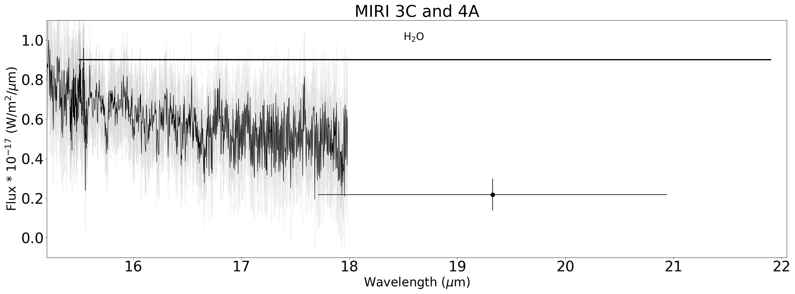
Past 18 $\mu$ m, the sensitivity of the MRS drops significantly due to a combination of low efficiency of the grating, low quantum efficiency of the detectors, and rising thermal background (Glasse et al., 2015). As a result the spectrum could not reliably be extracted in channel 4. Instead, the cube was collapsed from 17.71 to 20.94 $\mu$ m (Channel 4A) to produce a single photometric point. The source center is found by fitting a 2-D Gaussian to the collapsed channel 4A cube. A circular aperture (radius of 1.5 FWHM) is placed at the measured PSF center and the same aperture correction described above is used. We measure the background using an off-target reference aperture with the same radius and subtract the background.

The error in the extracted spectrum was estimated using the propagated error by the jwst pipeline Extract1dStep. The output x1d.fits files contain an ERR array extension that captures the error of the full processing chain, including the photon noise of the source. The extracted spectrum of the pipeline uses an annulus subtraction that introduces systematic errors form the background subtraction, but the overall spectrum matches the flux and shape of our own extraction. We therefore assume that the error reported by the pipeline should be representative for our own extraction. Indeed, the slope of the error follows the expected rising thermal background, but seems to be overall a factor of ten lower than what one would expect from the ETC. Additionally, comparing with the noise from a collection of reference apertures around the field of view confirms this discrepancy. We therefore choose to artificially amplify the pipeline estimated error by a factor of 10, yielding a rather conservative estimate of the S/N until the pipeline issue is resolved.

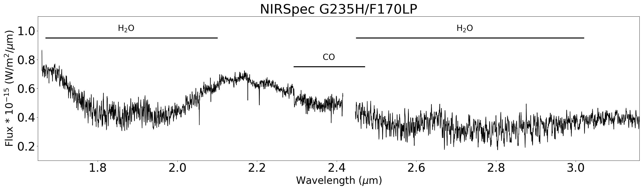
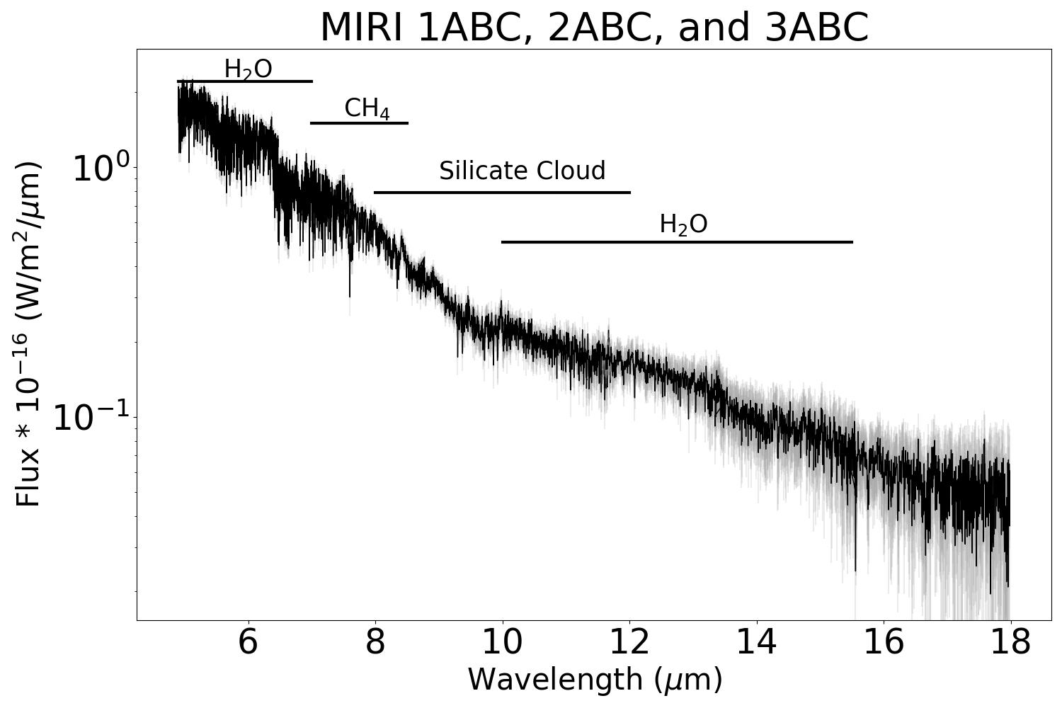
The full reduced spectrum with labeled bandpasses is shown in Figure 2. The NIRSpec (1 $\mu$ m - 5 $\mu$ m) spectra have a signal to noise of 50 - 400 per pixel. The MIRI (4.9 $\mu$ m - 20.94 $\mu$ m) spectra have a signal-to-noise of 7 to 20 per pixel, with hardly any signal in Channel 4 (17.66 $\mu$ m - 28.1 $\mu$ m). The photometry point from channel has a signal-to-noise of 2.7.

3.3 NIRSpec-MIRI Instrument Overlap

There are 557 data points from NIRSpec and 370 data points from MIRI that overlap in wavelength. When the NIRSpec data are binned down and interpolated onto MIRI’s wavelength spacing some portions of the NIRSpec data have a higher baseline flux, more than 3-sigma away from the MIRI data points. In Figure 3 shows the overlap region of NIRSpec IFU and MIRI MRS data at the resolution of each respective instrument.

4 Atmospheric Features

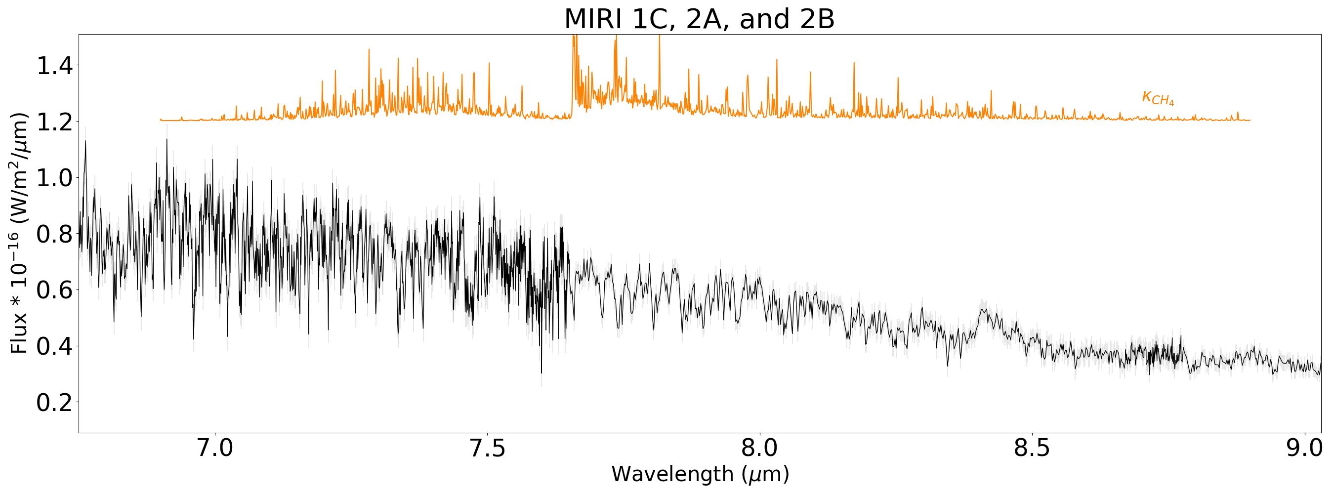
This spectrum is one of the highest signal-to-noise and broadest spectral coverage dataset of a brown dwarf or planetary mass companion to-date. With a spectral resolution up to $\sim$ 3000, a wealth of atmospheric molecular features are revealed. In this section, we visually identify absorption features in the spectra and in some cases compare them to molecular cross sections. In each subsection we discuss the molecules found and how they compare to similar brown dwarfs. The full VHS 1256 b spectrum displays several absorption features from atmospheric gases that have been previously observed in brown dwarf and extended mid-infrared coverage that can constrain methane, water, and carbon monoxide. There is evidence for carbon dioxide as well. Across the spectrum there are at least six detection regions of water, one visible methane feature, and two detections of carbon monoxide, which probe different pressure levels along the object’s pressure-temperature profile. From 8 $\mu$ m to 12 $\mu$ m the spectral slope shows evidence of a silicate cloud. These atomic, molecular, and cloud features are highlighted in Figures 4 and 5.

4.1 Near-Infrared Alkali Lines

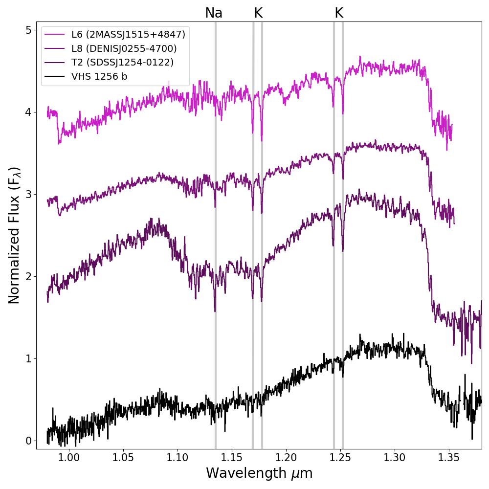
Late M dwarf stars and L spectral type brown dwarfs display absorption features from neutral gases such as vanadium oxide (VO), iron hydride (FeH), potassium (K), Titanium Oxide (TiO), and sodium (Na). These absorption features can be used to infer surface gravity. Broader and deeper absorption features from these molecules and atoms correspond to higher surface gravity and older ages (Allers & Liu, 2013; McGovern et al., 2004). The 1 $\mu$ m to 1.35 $\mu$ m portion of the JWST/NIRSpec spectrum (Top: Figure 4) holds two K doublets and a Na line that indicate a relatively low surface gravity, which is consistent with VHS 1256 b’s placement on a color-magnitude diagram. Figure 6 shows a comparison of VHS 1256 b’s Na and K lines with those of field brown dwarfs. Both absorption lines appear narrower than the same lines in a similar spectral type field brown dwarf, indicating a low surface gravity for VHS 1256 b. The first published near-infrared spectrum of VHS 1256 b in Gauza et al. (2015) showed no K doublet features and no detection of the 1.134 $\mu$ m Na line, possibly due to insufficient resolution. Follow-up work by Petrus et al. (2022) obtained medium resolution (R $\sim$ 8,000) spectra of VHS 1256 b, at a resolution higher than the JWST spectrum presented here. The Na line at 1.134 $\mu$ m and K doublets at 1.173 $\mu$ m and 1.248 $\mu$ m are easier to distinguish from the continuum in the JWST spectrum, however the published spectrum from Petrus et al. (2022) likely has the resolution to capture a broader range of absorption features such as Fe, FeH, and TiO. However, the standard NIRSpec pipeline procedures are still in development. Once these parameters have been refined, future reductions of the JWST spectrum may lead to the detection of finer features with higher signal-to-noise ratios.

4.2 Water

All spectral types of brown dwarfs possess absorption features due to water vapor in the near and mid-infrared. The shape and depth of these features are primarily determined by the effective temperature or spectral type of a brown dwarf (Allers & Liu, 2013). Previously published space-based spectroscopic infrared observations of VHS 1256 b and other brown dwarfs are sensitive to water but often limited to resolutions of a few hundred (Zhou et al., 2020). The sensitivity and added resolution of the JWST data provide crucial details regarding the presence of water vapor in the atmospheres of brown dwarfs. Water absorption bands are present in the VHS 1256 b spectrum at 1.3 $\mu$ m - 1.6 $\mu$ m, 1.7 $\mu$ m - 2.1 $\mu$ m, and shape the spectrum beyond 10 $\mu$ m. Water overlaps with carbon monoxide (CO) between 2.2 $\mu$ m and 2.6 $\mu$ m and between 4.3 $\mu$ m and 5 $\mu$ m. All water features are labeled in Figures 4 and 5.

4.3 Methane

Brown dwarfs below an effective temperature of $\sim$ 1400 K begin to display methane absorption features, as methane is favored in the chemical reaction between methane and carbon monoxide at these temperatures (Lodders & Fegley, 2002). Methane absorption at 1.67 $\mu$ m is also a typical T-dwarf signature (Cushing et al., 2005).

We have an absorption feature in the spectrum at 1.66 $\mu$ m in VHS 1256 b, however this feature is slightly blue-ward of the typical 1.67 $\mu$ m location, but also too broad to be FeH absorption that is seen in warmer L-dwarfs (Cushing et al., 2005). This feature also coincides with excess amplitudes from oscillations in the extracted dithers at wavelengths between 1.65 $\mu$ m and 1.75 $\mu$ m. Only dithers 2 and 3 of the total four show no oscillations in the extracted spectra, but the slight depression remains when only using dither 2 and 3 of the observations. The crest-to-crest width of the oscillation waves in the calibrator star between 1.65 $\mu$ m and 1.75 $\mu$ m is $\sim$ .01 $\mu$ m - .02 $\mu$ m, and the width of the potential methane feature is .02 $\mu$ m. Previously published near-infrared spectra show no methane absorption at 1.67 $\mu$ m (Petrus et al., 2022; Gauza et al., 2015). If this feature remains after further pipeline updates the opacity source causing this feature will need to be validated with further atmospheric modeling work.

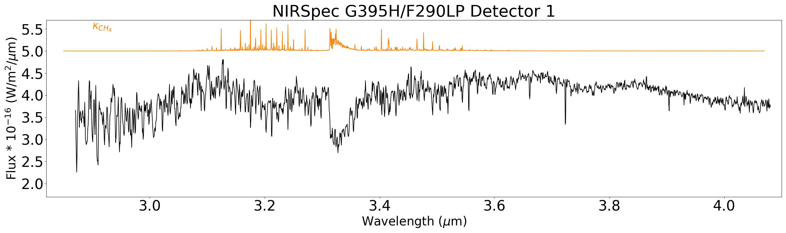
We also find a relatively shallow methane feature between 2.8 $\mu$ m and 3.8 $\mu$ m that is consistent with the previously published L-band spectrum in Miles et al. (2018). Methane absorption at $\sim$ 3.3 $\mu$ m is more prominent in brown dwarfs than methane absorption at 1.65 $\mu$ m, and is seen even in mid-L-dwarfs (Noll et al., 2000). In this effective temperature range, methane has a significant opacity contribution between 7 $\mu$ m and 9 $\mu$ m, but its overall strength compared to water and other molecules is smaller. This region does not visually mirror the predicted opacity profile of methane for this reason.

All of the near-infrared and mid-infrared methane features appear depleted relative to similar temperature brown dwarfs, indicating that disequilibrium chemistry is influencing the apparent abundance of methane in the upper atmosphere. We will discuss the degree of atmospheric mixing required to recreate these methane features with models in Section 5.

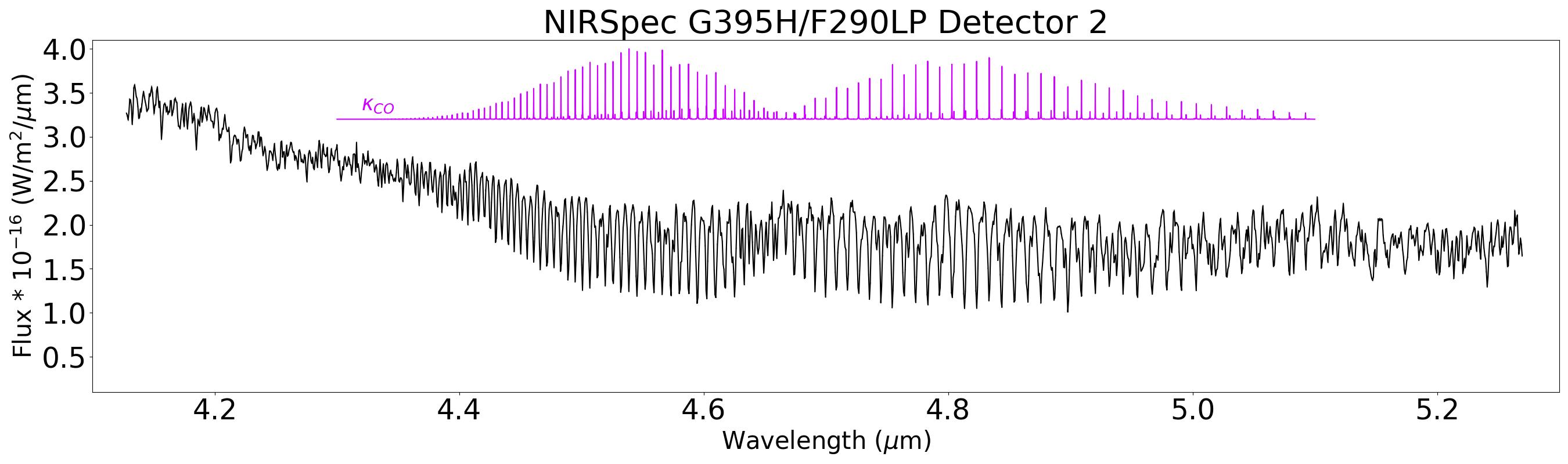
4.4 Carbon Monoxide

Carbon monoxide (CO) is a common near-infrared spectral feature in very low mass stars and brown dwarfs with effective temperatures above $\sim$ 1400 K (Lodders & Fegley, 2002; Cushing et al., 2005). Carbon monoxide produces a strong feature centered at 4.6 $\mu$ m in warm brown dwarfs. Cooler brown dwarfs that have disequilibrium chemistry driven by atmospheric mixing (Sorahana & Yamamura, 2012) also display this feature. VHS 1256 b’s effective temperature is cool enough where a small degree of carbon monoxide will be detected at 2.3 $\mu$ m. The depth and shape of the central feature is similar to previously published K-band spectra in Hoch et al. (2022) and Petrus et al. (2022). We also detect a densely packed set of carbon monoxide features around 4.6 $\mu$ m in VHS 1256 b’s spectrum. It is the best resolved, highest signal-to-noise, set of features from the fundamental carbon monoxide bandhead compared to previously published space-based brown dwarfs spectra and photometry from AKARI (Sorahana & Yamamura, 2012) and Spitzer (Patten et al., 2006).

4.5 Carbon Dioxide

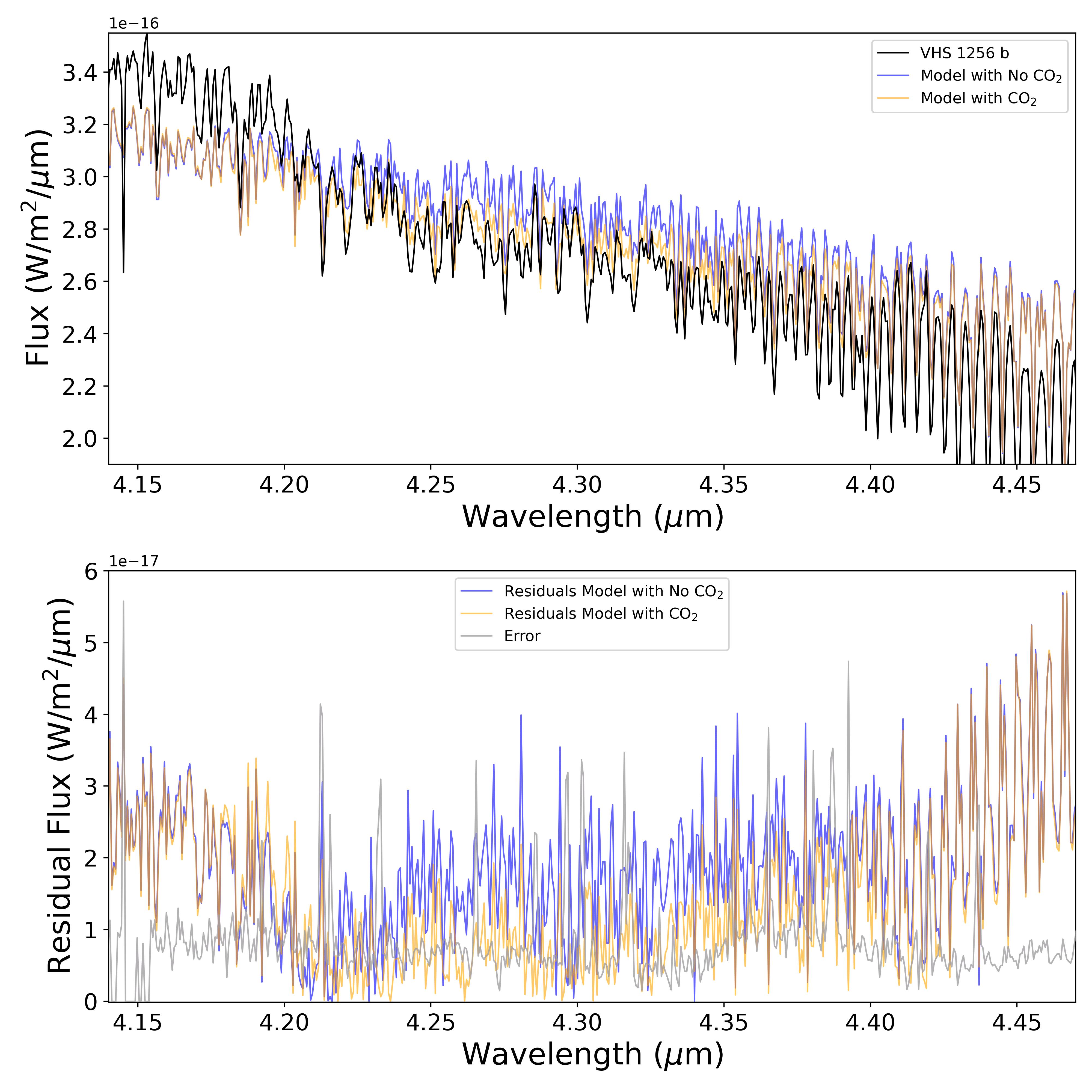
Carbon dioxide (CO₂) is another carbon- and oxygen-bearing gas that can provide insight into metallicity or atmospheric effective temperature (Tsuji et al., 2011; Sorahana & Yamamura, 2012; Lodders & Fegley, 2002). The CO₂ feature at 4.2 $\mu$ m is inaccessible from ground-based observatories and has only been detected in a handful of mid-infrared observations of T-type brown dwarfs (Tsuji et al., 2011; Sorahana & Yamamura, 2012). We show evidence for this CO₂ feature in the JWST spectrum of VHS 1256 b by comparing two versions of an atmospheric model, one with CO₂ opacities added and one without, as shown in Figure 7. The model comparisons reveal a slight absorption feature where CO₂ influences the spectrum from 4.2 $\mu$ m to 4.4 $\mu$ m. In M-dwarfs and relatively warm L-dwarfs, CO₂ is theorized to primarily trend with effective temperature, while at lower effective temperatures where methane should be the dominant carbon-bearing gas CO₂ will vary with both atmospheric pressure and temperature (Lodders & Fegley, 2002). The presence of CO₂ in VHS1256 b’s spectrum would not be not surprising, but needs to be verified with more detailed atmospheric analysis.

4.6 Clouds

The transition between red to blue near-infrared colors at the L-to-T transition shown in Figure 1 is likely driven by the condensation and eventual descent below the photosphere of silicate grains composed of enstatite, forsterite, or quartz as these objects cool. Low surface gravity brown dwarfs and directly imaged exoplanets can retain their silicate clouds at lower effective temperatures, producing their redder colors compared to field counterparts. VHS 1256 b displays a significant silicate cloud feature in the JWST/MIRI spectrum from 8 $\mu$ m to 11 $\mu$ m when compared to a standard brown dwarf and the relatively red brown dwarf 2MASSW J2224438-015852 (2M2224-0158) discovered in Kirkpatrick et al. (2000), that is an outlier along the L-to-T transition (Figure 11). Compared to 2M2224-0158, VHS 1256 b shares the same spectral shape across 8 $\mu$ m to 11 $\mu$ m indicating an absorption feature due to silicate clouds of a similar composition. The best fit cloud model for 2MASS 2224-0158 from Burningham et al. (2021) was a combination of enstatite (MgSiO₃), quartz (SiO₂), and a higher pressure iron (Fe) cloud.

4.7 Other Molecular Gases and Clouds

VHS 1256 b’s spectrum shows evidence of disequilibrium chemistry based on methane and carbon monoxide, therefore we explored the potential presence of other disequilibrium molecules.

From the equilibrium Sonora Bobcat models (Marley et al., 2021), we scaled different molecular abundances to search for species that could appear in dis-equilibrium conditions. In VHS 1256 b’s spectrum, there are no obvious signs of acetylene (C₂H₂), ethylene (C₂H₄), ethane (C₂H₆), hydrogen sulfide (H₂S), phosphine (PH₃), or hydrogen cyanide (HCN). Outside of the features listed prior to this subsection, more detailed analysis and approaches such as retrievals and cross correlation will need to be applied to the JWST VHS 1256 b spectra to fully understand the object’s atmospheric chemistry.

5 Atmospheric Modeling

We used the long-developed EGP substellar code (Marley et al., 1996, 2012; Fortney et al., 2005, 2007, 2008; Morley et al., 2014; Marley et al., 2021; Karalidi et al., 2021; Mukherjee et al., 2022) to find the best-fit forward model for the observed JWST spectrum. This lineage of codes parametrizes the cloudiness of an object using the sedimentation parameter $f_{\rm sed}$ and parameterizes the mixing strength using the eddy diffusion coefficient K_zz (Ackerman & Marley, 2001). A higher value of $f_{\rm sed}$ describes less optically thick clouds with larger particles: lower values produce thicker clouds with smaller particles. The eddy diffusion coefficient K_zz has higher values if atmospheric mixing is strong, potentially driving the atmosphere out of chemical equilibrium (Hubeny & Burrows, 2007; Saumon et al., 2006) and also extending the extent of atmospheric cloud decks. The goal of our atmospheric modeling efforts is to capture the prominent atmospheric physics and chemistry that influences the spectrum of VHS 1256 b and the EGP family of codes is well-suited to this task, although modeling VHS 1256 b’s full spectrum required careful fine tuning of parameters to capture the object’s disequilibrium chemistry and cloudiness.

We used PICASO 3.0 (Mukherjee et al., 2022), a modified Python version of the Fortran-based EGP code that includes the capability of self-consistently modeling both disequilibrium chemistry and clouds simultaneously with a pressure-dependent K_zz profile. The details of the code are described in Mukherjee et al. (2022), used opacity sources are detailed in Table 3 in Mukherjee et al. (2022). We first explored a small grid with temperatures running from 900 K to 1600 K at intervals of 100 K and $f_{\rm sed}$ values of 1, 2, 3, and 8. Each atmospheric model has 90 layers spaced in atmospheric pressure. The spectra were post processed to mirror abundances of an atmosphere with two different uniform K_zz profile values, 10⁵ cm² s^-1 and 10⁸ cm² s^-1. The smaller value of K_zz corresponds to the theoretical estimated K_zz (Zahnle & Marley, 2014) value and the higher value matches previously published mixing values estimated from the 3 $\mu$ m methane feature in Miles et al. (2018). The best attempt at a fine-tuned model that matches the overall shape of the spectrum had parameters T ${}_{\rm eff}=$ 1100 K, $f_{\rm sed}=$ 1, log(g) = 4.5, and K ${}_{zz}=$ 10⁸ cm² s^-1. However, the best fit model from this initial grid produced too much flux in the near-infrared despite matching the majority of the molecular absorption features. The estimated temperature is similar to effective temperatures (1122 $\pm$ 16K and 1171 $\pm$ 17 K), derived in Dupuy et al. (2022) using atmospheric evolution models from Saumon & Marley (2008). Our forward modeling approach produces lower effective temperatures compared to the forward model derived effective temperatures in Hoch et al. (2022) (1200 K) and Petrus et al. (2022) (1380 K) but higher than the temperature derived in Zhou et al. (2020) (1000 K).

In order to better fit the observed near-infrared flux, we adopted a two–cloud model and added a self consistent treatment of atmospheric mixing to estimate K_zz as a function of pressure. This modeling approach in PICASO 3.0 simultaneously includes the heating/cooling due to clouds and mixing induced disequilibrium chemistry while calculating the atmospheric structure of the object. Instead of a single cloud with an $f_{\rm sed}$ of 1, we used a mixture of two clouds, with 90 $\%$ of the modeled clouds having $f_{\rm sed}$ = 0.6 and 10 $\%$ of the modeled clouds having $f_{\rm sed}$ = 1.0. The clouds described by the lower $f_{\rm sed}$ = 0.6 value produce a thicker, deeper cloud layer that helps match the model to the observed spectral shape of VHS 1256b. The fluxes for each of these cloudy disequilibrium chemistry models were first calculated separately and were then linearly combined using,

F_{total}=fF_{1}+(1-f)F_{2}

(1)

to obtain the total flux ( $F_{total}$ ) which is shown in Figure 8. In Equation 1, $f$ represents the fractional coverage of one of the cloudy models, $F_{1}$ and $F_{2}$ represents the fluxes calculated from models with clouds with a particular $f_{\rm sed}$ . The use of two clouds is motivated by the object’s measured variability, which is caused by changes in the surface brightness potentially created by moving cloud patches. Using a self consistent and pressure dependent approach to estimate atmospheric mixing, we find K_zz values ranging from 10⁸ cm² s^-1 to 10⁹ cm² s^-1 along the pressure temperature profile. The best fit spectrum using these parameters is shown in Figure 8 and the atmospheric profile and chemistry are described in Figure 9.

The best fit atmospheric model matches the overall shape of the 1 $\mu$ m - 20 $\mu$ m spectrum of VHS 1256 b with discrepancies occurring where the silicate cloud feature appears and also around the peak from 1.5 $\mu$ m to 1.8 $\mu$ m, where the spectrum is shaped by water and collisionally induced absorption from hydrogen. The major equilibrium and disequilibrium absorption features described in section 4 are not exactly matched and dampened because of atmospheric clouds. The chemical abundance profile of the best fit model demonstrates that water and carbon monoxide are relatively insensitive to atmospheric mixing. The volume mixing ratios of methane, ammonia, and carbon dioxide are affected by atmospheric mixing, however, based on Section 4, only carbon dioxide and methane produce visible spectral features.

6 Discussion

6.1 Bolometric Luminosity and Mass

Integrating over VHS 1256 b’s JWST spectrum and using the best fit model described in the previous section to estimate flux from wavelength ranges not covered by our JWST spectrum, we find a bolometric luminosity of $log\left(\frac{L_{bol}}{L_{\odot}}\right)$ = -4.55 $\pm$ 0.009, adopting the Gaia Early Data Release 3 distance measurement to the system of 21.15 $\pm$ 0.22 pc (Gaia Collaboration et al., 2021). Our JWST spectrum covers most of the full luminous range of VHS 1256b; 98 $\%$ of the measured luminosity is derived directly from the spectrum, with only 2 $\%$ extrapolated from model fits to wavelengths outside of our JWST wavelength coverage. So much of the SED is covered by measurements and so many independent bands are included that the statistical/random error on our bolometric luminosity value is very small. With a precise distance measurement from Gaia Collaboration et al. (2021) for this system, the most significant uncertainty will stem from the absolute flux calibration of the spectrum using the A3V star TYC 4433-1800-1 (see Section 3). Over the course of the JWST’s operation a dedicated absolute flux calibration program is planned to enable better than 2 $\%$ flux calibration over a wide range of objects (Gordon et al., 2022). Thus, to set the error on our bolometric luminosity measurement at the current early stage of the JWST mission, we estimate a conservative error on the absolute flux calibration of 3 $\%$ and add this in quadrature with the error on the integrated spectrum.

Adopting the Gaia DR3 distance for the system, a spectral type of L7 $\pm$ 1.5 and the VISTA Hemisphere survey $K_{S}$ photometry from Gauza et al. (2015), and a bolometric correction $BC_{Ks}$ based on the polynomial relationship for young M to T type objects from Filippazzo et al. (2015), we find a photometric bolometric luminosity of $log\left(\frac{L_{bol}}{L_{\odot}}\right)$ = -4.60 $\pm$ 0.05, in good agreement with the value derived from our JWST spectroscopy. However, recent bolometric luminosity estimates from ground-based, near-IR spectroscopy for VHS 1256 b are slightly fainter than the value we find with JWST: Hoch et al. (2022) find a best value of $log\left(\frac{L_{bol}}{L_{\odot}}\right)$ = -4.67, within a range from -4.6 to -4.7, while Petrus et al. (2022) find $log\left(\frac{L_{bol}}{L_{\odot}}\right)$ = -4.67 $\pm$ 0.07. The bolometric luminosity estimate from Petrus et al. (2022) adopts a distance of 22.2 ${}^{+1.1}_{-1.2}$ pc from (Dupuy et al., 2020), rather than the more accurate Gaia eDR3 measurement. Adjusting to the Gaia distance measurement leads to a slightly smaller bolometric luminosity, further increasing the tension between the JWST measurement and ground-based spectroscopic measurements.

Dupuy et al. (2022) determine an updated age for the system of 140 $\pm$ 20 Myr from dynamical masses derived from orbital fits to the inner AB binary. VHS 1256 b sits close to the deuterium burning limit – if VHS 1256b is slightly above the deuterium burning limit, it will be actively burning deuterium at this age. For the short duration of its deuterium burning phase, a lower mass object may be more luminous than a higher mass object at the same age, see Figure 10. As a given luminosity can correspond to a range of masses in this case, direct interpolation from this model grid can produce erroneous mass estimates.

To robustly estimate the mass of VHS 1256 b, we implemented a rejection sampling method similar to that described in Dupuy et al. (2022). First, we draw 1 $\times$ 10⁶ samples of age and mass from a Gaussian distribution in age around 140 Myr, with $\sigma$ =20 Myr, and a uniform distribution in mass from 1 to 50 M_Jup. For each age, mass sample we then interpolate a model luminosity from an evolutionary model grid, and calculate $\chi^{2}$ as: $\chi^{2}=\frac{(L_{\rm bol,model}-L_{\rm bol,measured})^{2}}{\sigma_{\rm Lbol,measured}^{2}}$ , then convert to a probability ( $P$ ) by normalizing by the minimum $\chi^{2}$ ( $P=e^{-\frac{\chi^{2}-\chi_{min}^{2}}{2}}$ ) value among our 1 $\times$ 10⁶ samples. For each sample, we also draw a uniformly distributed number from 0 to 1. We retain the samples where the sample probability is greater than the uniformly distributed variate drawn for that sample.

As VHS 1256b has strong evidence for the presence of clouds in its spectrum from the detection of the silicate feature at 10 $\mu$ m, we implemented this rejection sampling procedure using the hybrid cloud grid of Saumon & Marley (2008), which includes clouds for objects with L-type spectra and clear atmospheres for objects with T-type spectra.

A histogram of the final set of accepted masses are shown in Figure 10. We find a bimodal distribution of masses, with accepted samples both above and below the deuterium mass burning limit, as also seen in Dupuy et al. (2022). The percentage of samples which fall into each of the two peaks depends strongly on the both the bolometric luminosity value and the uncertainty on that value. While we cannot conclusively determine whether VHS 1256b falls above or below the deuterium mass burning limit, all accepted samples for this model have masses $<$ 20 M_Jup.

6.2 Variability

Young, planetary mass objects with mid-to-late-L spectral types are highly variable in the near-IR (Biller et al., 2015, 2018; Lew et al., 2016; Bowler et al., 2020; Zhou et al., 2020), with variability amplitudes $>$ 5 $\%$ over observations a few hours in length. VHS 1256 b is the most variable of this cohort. Over a contiguous six-orbit observation with HST/WFC3 obtained in 2018, Bowler et al. (2020) found that VHS 1256 b varied by $>$ 20 $\%$ between 1.1 to 1.7 $\mu$ m over 8 hours. In the near-IR, Bowler et al. (2020) fit the observed HST trend with a single sinusoidal model, however, in an additional 15-orbit / 42 hour HST / WFC3 observation in 2020 presented by Zhou et al. submitted, the variability observed is more complex, requiring a 3-sinusoid + slope model for a full fit. In the mid-IR, Zhou et al. (2020) obtained a contiguous 36-hour Spitzer 4.5 $\mu$ m lightcurve of VHS 1256 b and found a best fit model for this lightcurve of a single sinusoid with a period of 22.04 $\pm$ 0.05 hours (interpreted as the rotation period of the object) and a peak-to-peak amplitude of 5.76 $\pm$ 0.04 $\%$ , a significantly lower variability amplitude when compared to the near-IR variability. Both the near-IR and mid-IR variability are likely driven by patchy thin and thick silicate clouds (Apai et al., 2013). Variability is an important probe of the inhomogeneity of the top-of-atmosphere structure of these objects and it is critical to understand the intrinsic variability of this target in order to interpret our JWST observations. To do so, we have conducted a multi-telescope, multi-epoch photometric variability monitoring campaign starting in February 2022 and continuing through July, directly covering the JWST observation epoch, which will be presented in Biller et al. in prep.

However, over the $\sim$ 4 hour timescale of our ERS observations, we expect a relatively low level of variability, based on estimates from the earlier HST and Spitzer observations. To estimate the range of potential variability we expect during the NIRSpec observation, we drew 10000 sample 2-hour observations from the 3-sinusoid model from Zhou et al. (2022), and estimated the intrinsic variability occurring during each simulated observation as the maximum minus the minimum value from the model during that time span. We used a very fine time sampling and did not realistically simulate noise or the actual cadence of our JWST observations. Thus, this method constrains the intrinsic variability and the actual measurement of variability in any given observation would yield a smaller value than these predictions. From our simulated observations, 50 $\%$ of samples varied by less than 1.5 $\%$ , 75 $\%$ of samples varied by less than 2.5 $\%$ , and 95 $\%$ of samples varied less than 3.7 $\%$ . For wavelengths $>$ 3 $\mu$ m, drawing 10000 sample 2-hour observations from the single sinusoid model used to fit the Spitzer 4.5 $\mu$ m lightcurve from Zhou et al. (2020), 50 $\%$ of samples varied by less than 1.1 $\%$ , 75 $\%$ of samples varied by less than 1.5 $\%$ , and 100 $\%$ of samples varied by less than 1.6 $\%$ . More conservatively, we estimate a maximum potential variability measurement of 5 $\%$ over 2 hours for the JWST/NIRSpec 1-3 $\mu$ m observations, based on the highest amplitude variability epoch, where VHS 1256 b displayed 20 $\%$ variability over 8 hours (Bowler et al., 2020). Assuming the same scaling between near-IR and mid-IR lightcurves as found between the HST and Spitzer lightcurves of Bowler et al. (2020) and Zhou et al. (2020), we estimate a maximum potential variability measurement of 1.5 $\%$ over 2 hours at wavelengths $>$ 3 $\mu$ m. Variability has not been measured beyond 5 $\mu$ m for any planetary mass object, but assuming a continuing trend of decreasing variability amplitude with increasing wavelength, we expect variability at wavelengths $>$ 5 $\mu$ m to be negligible.

6.3 Atmospheric Chemistry

The JWST spectrum has molecular features that are consistent with previous findings of VHS 1256 b and other young, red late L-dwarfs having atmospheres that are out of chemical equilibrium (Chauvin et al., 2004; Gauza et al., 2015; Liu et al., 2016; Miles et al., 2018). The presence of CO absorption and depleted CH₄ absorption compared to equilibrium atmospheric models, supports atmospheric mixing forcing the atmosphere into chemical disequilibrium. The CH₄ absorption feature at 3.3 $\mu$ m is the most prominent absorption feature stemming from disequilibrium chemistry in VHS 1256 b’s spectrum and potentially other similar temperature directly imaged exoplanets. The fine tuned forward model shown in Figure 8 has an associated CH₄ abundance profile (Figure 9), but the model does not match the 3.3 $\mu$ m CH₄ feature or many other molecular features along the spectrum, despite matching the overall SED shape. For sedimentation parameter values of $f_{\rm sed}$ = 4, CH₄ features at 1.6 $\mu$ m and 7 $\mu$ m appear in model spectra, but for our best fit model with $f_{\rm sed}$ $<$ 1, these features are quite muted. The estimated K_zz range of VHS 1256 b spans 10⁸ cm² s^-1 - 10⁹ cm² s^-1, which is consistent with the estimated K_zz of 10⁸ cm² s^-1 from Miles et al. (2018). However, not matching crucial disequilibrium absorption features is significant and means future modeling work on clouds and mixing will need to be done to estimate a meaningful K_zz for VHS 1256 b.

We show evidence of CO₂ being useful for reproducing the shape of the JWST spectrum at 4.2 $\mu$ m as shown in Figure 7 and 9. The portions of the JWST spectrum surrounding the CO₂ feature are discrepant from the best fit atmospheric model. CO₂ is also influenced by disequilibrium chemistry, but the timescale of CO₂’s conversion from CH₄ is much faster than the conversion of CO to CH₄ (Zahnle & Marley, 2014), therefore CO₂ quenches at higher atmospheric pressures. Historically, disequilibrium chemistry driven by atmospheric mixing has only been detectable from a single molecule in exoplanets and brown dwarfs: either CH₄ for warmer L-dwarfs or CO for cooler T-dwarfs. JWST has the capability to confidently detect two different molecular gases with different quench pressures between 1 $\mu$ m and 5 $\mu$ m. JWST is capable of detecting CO₂ and CH₄ or CO over the entire L, T, and potentially Y-dwarf sequence, revolutionizing our understanding of disequilibrium chemistry as traced by carbon species in the atmospheres of brown dwarfs and extrasolar planets.

6.4 Silicate Clouds

Brown dwarfs are expected to have clouds in their photospheres as their temperatures drop below the condensation curves of various species (Lunine et al., 1986, 1989; Tsuji et al., 1996; Chabrier et al., 2000; Ackerman & Marley, 2001). There are several lines of evidence for clouds in brown dwarfs, including:

•

The red colors of L-type brown dwarfs, which quickly transition to blue colors as the brown dwarfs cool through the L-to-T transition and clouds are theorized to sink below the visible atmosphere (Kirkpatrick et al., 1999; Allard et al., 2001; Saumon & Marley, 2008)
•

The variability seen in brown dwarfs (Artigau et al., 2009; Metchev et al., 2015), which is most prominent near the L-to-T transition and can be modeled with patchy clouds (Apai et al., 2013; Radigan et al., 2012; Burgasser et al., 2002; Saumon & Marley, 2008)
•

The match in temperature between condensation curves and kinks in brown dwarf color-magnitude diagrams (Fegley & Lodders, 1994; Lodders, 1999; Morley et al., 2012; Leggett et al., 2015).

There are also alternative explanations for the previous phenomena, such as temperature-pressure profiles that have been perturbed by disequilibrium chemistry (Tremblin et al., 2015).

Solid state spectroscopic features can be unambiguous signatures of clouds. At VHS 1256 b’s temperature, the most prominent feature is expected to be from silicate particles, which have a broad 10 $\mu$ m feature that is commonly seen in the interstellar medium and in the disks of young stars (Draine & Lee, 1984). Using the Spitzer Infrared Spectrograph, Cushing et al. (2006) detected a “plateau”-shaped absorption feature from 9-11 $\mu$ m in the spectra of several mid-L brown dwarfs, which they attributed to small amorphous silicate particles. A compendium of all of the Spitzer spectra of brown dwarfs shows that silicate features are common, but not ubiquitous, for L2-L8 brown dwarfs (Suárez & Metchev, 2022).

The JWST/MIRI spectrum of VHS 1256 b shows a prominent silicate feature compared to the Spitzer brown dwarfs, with a shape that is well-matched to 2M2224-0158 (see Figure 11). Burningham et al. (2021) modeled the spectrum of 2M2224-0158 and found a best-fit with clouds composed of sub-micron enstatite/silicate, quartz, and iron. The presence of a prominent silicate feature in VHS 1256 b is strong evidence for small particles. Detailed modeling of the cloud composition and grain size distribution will be the subject of a future paper.

Various groups have developed models for clouds in brown dwarfs and exoplanets, but they tend to focus on fitting the near-infrared (1-2 $\mu$ m) part of the spectrum, where extinction from large particles (10-100 $\mu$ m) mute the spectral features (Chabrier et al., 2000; Allard et al., 2001; Saumon & Marley, 2008; Madhusudhan et al., 2011). It has long been known (e.g., from the comet literature), small particles contribute less to extinction (Gao et al., 2018), but they result in a much more prominent 8-12 $\mu$ m silicate feature (Min et al., 2004). JWST’s broad wavelength coverage allows us to constrain both populations of cloud particles.

7 Summary

VHS 1256 b has several qualities that distinguish it from the typical brown dwarfs that form the L-to-T sequence shown in Figure 1:

1.

VHS 1256 b is a young, low-mass object that has the characteristic red colors seen in other low-gravity objects (see Sections 1 and 6.1).
2.

VHS 1256 b has the largest amplitude of variability of any substellar object to date (see Section 6.2).
3.

VHS 1256 b shows disequilibrium chemistry caused by turbulent, vertical mixing (see Section 6.3).
4.

VHS 1256 b has a prominent silicate feature indicating the presence of small cloud particles (see Section 6.4).

Previous works have drawn physical connections between some of these qualities. Young, low-mass brown dwarfs have red colors (Liu et al., 2016; Faherty et al., 2016). These same objects are more likely to have large amplitude variability (Biller et al., 2015; Lew et al., 2016; Vos et al., 2017, 2019; Bowler et al., 2020) and to show disequilibrium chemistry (Barman et al., 2011; Zahnle & Marley, 2014; Miles et al., 2018). Cloud models predict that turbulence and vertical mixing produce differentiated clouds with small particles at the top (Ackerman & Marley, 2001; Helling & Woitke, 2006; Helling et al., 2006; Gao et al., 2018), and objects that are reddened by extinction from large grains are more likely to have 10 $\mu$ m silicate features from small grains (Suárez & Metchev, 2022). Turbulent mixing is also likely to induce variability for objects of VHS 1256 b’s temperature, which are expected to have cloudy and cloud-free regions (Radigan et al., 2012; Apai et al., 2013). Together, these properties paint a picture of a highly dynamic atmosphere, where turbulent convection drives both disequilibrium chemistry and the upwelling of condensible gasses, which form patchy silicate clouds that drive planetary variability.

8 Conclusions

We reduced JWST NIRSpec IFU and MIRI MRS early release science observations of VHS 1256 b to produce the best spectrum of a planetary-mass object to date at medium resolution covering 0.97 $\mu$ m - 19.8 $\mu$ m. The sensitivity (NIRSpec: SNR $\sim$ 50 - 400, MIRI: SNR $\sim$ 7 - 20) and broad wavelength coverage of the data enabled the identification of several medium-resolution features such as water, methane, carbon monoxide, carbon dioxide, and silicate clouds within the atmosphere of VHS 1256 b. The data have sufficient signal-to-noise for forward modeling analysis to estimate the cloudiness, chemical abundance profiles, and strength of atmospheric mixing of VHS 1256 b. Our best attempt at matching the 0.97 $\mu$ m - 19.8 $\mu$ m spectra required combining two relatively thick cloud decks (90 $\%$ $f_{\rm sed}$ = .6 and 10 $\%$ $f_{\rm sed}$ = 1), low surface gravity (log(g) = 4.5), radius of 1.27 R_Jup, and an effective temperature of 1100 K. The derived K_zz profile of VHS 1256 b changes from 10⁸ cm² s^-1 - 10⁹ cm² s^-1, with stronger mixing generally occurring lower in the atmosphere. The best attempt model matches the overall shape of the spectrum, but does not adequately capture molecular absorption features typically used to estimate K_zz. The luminosity of VHS 1256 b was measured to within less than a percent ( $\mathrm{l}og(L_{bol}/L_{\odot})$ = -4.55 $\pm$ 0.009), robustly providing an upper mass limit of 20 M_Jup for VHS 1256 b. These initial results from the JWST early release science observations are groundbreaking and also obtainable for numerous other nearby brown dwarfs that will be observed in future observation cycles. This observatory will be a trailblazer, pushing our understanding of atmospheric physics in planetary-companions, brown dwarfs, and exoplanets for years to come.

9 Acknowledgements

This project was supported by a grant from STScI (JWST-ERS- 01386) under NASA contract NAS5-03127. This work benefited from the 2022 Exoplanet Summer Program in the Other Worlds Laboratory (OWL) at the University of California, Santa Cruz, a program funded by the Heising-Simons Foundation. MBo acknowledges support in France from the French National Research Agency (ANR) through project grant ANR-20-CE31-0012. This project has received funding from the European Research Council (ERC) under the European Union’s Horizon 2020 research and innovation programme (COBREX; grant agreement n^∘ 885593; EPIC, grant agreement n^∘ 819155). This work has benefited from The UltracoolSheet at http://bit.ly/UltracoolSheet, maintained by Will Best, Trent Dupuy, Michael Liu, Rob Siverd, and Zhoujian Zhang, and developed from compilations by Dupuy & Liu (2012); Dupuy & Kraus (2013); Liu et al. (2016); Best et al. (2018, 2021). S-P acknowledges the support of ANID, – Millennium Science Initiative Program – NCN19_171. S.M. is supported by a Royal Society University Research Fellowship. C.D. acknowledges financial support from the State Agency for Research of the Spanish MCIU through the “Center of Excellence Severo Ochoa” award to the Instituto de Astrofísica de Andalucía (SEV-2017-0709) and the Group project Ref. PID2019-110689RB-I00/AEI/10.13039/501100011033. B.B. acknowledges funding by the UK Science and Technology Facilities Council (STFC) grant no. ST/M001229/1.

References

Ackerman & Marley (2001) Ackerman, A. S., & Marley, M. S. 2001, ApJ, 556, 872, doi: 10.1086/321540
Allard et al. (2001) Allard, F., Hauschildt, P. H., Alexander, D. R., Tamanai, A., & Schweitzer, A. 2001, ApJ, 556, 357, doi: 10.1086/321547
Allers & Liu (2013) Allers, K. N., & Liu, M. C. 2013, ApJ, 772, 79, doi: 10.1088/0004-637X/772/2/79
Apai et al. (2021) Apai, D., Nardiello, D., & Bedin, L. R. 2021, ApJ, 906, 64, doi: 10.3847/1538-4357/abcb97
Apai et al. (2013) Apai, D., Radigan, J., Buenzli, E., et al. 2013, ApJ, 768, 121, doi: 10.1088/0004-637X/768/2/121
Apai et al. (2017) Apai, D., Karalidi, T., Marley, M. S., et al. 2017, Science, 357, 683, doi: 10.1126/science.aam9848
Argyriou et al. (2020) Argyriou, I., Wells, M., Glasse, A., et al. 2020, A&A, 641, A150, doi: 10.1051/0004-6361/202037535
Artigau et al. (2009) Artigau, É., Bouchard, S., Doyon, R., & Lafrenière, D. 2009, ApJ, 701, 1534, doi: 10.1088/0004-637X/701/2/1534
Baraffe et al. (2015) Baraffe, I., Homeier, D., Allard, F., & Chabrier, G. 2015, A&A, 577, A42, doi: 10.1051/0004-6361/201425481
Barman et al. (2011) Barman, T. S., Macintosh, B., Konopacky, Q. M., & Marois, C. 2011, ApJ, 733, 65, doi: 10.1088/0004-637X/733/1/65
Best et al. (2021) Best, W. M. J., Liu, M. C., Magnier, E. A., & Dupuy, T. J. 2021, AJ, 161, 42, doi: 10.3847/1538-3881/abc893
Best et al. (2018) Best, W. M. J., Magnier, E. A., Liu, M. C., et al. 2018, ApJS, 234, 1, doi: 10.3847/1538-4365/aa9982
Biller et al. (2015) Biller, B. A., Vos, J., Bonavita, M., et al. 2015, ApJ, 813, L23, doi: 10.1088/2041-8205/813/2/L23
Biller et al. (2018) Biller, B. A., Vos, J., Buenzli, E., et al. 2018, AJ, 155, 95, doi: 10.3847/1538-3881/aaa5a6
Boccaletti et al. (2015) Boccaletti, A., Lagage, P. O., Baudoz, P., et al. 2015, PASP, 127, 633, doi: 10.1086/682256
Boccaletti et al. (2022) Boccaletti, A., Cossou, C., Baudoz, P., et al. 2022, arXiv e-prints, arXiv:2207.11080. https://arxiv.org/abs/2207.11080
Bohlin et al. (2020) Bohlin, R. C., Hubeny, I., & Rauch, T. 2020, AJ, 160, 21, doi: 10.3847/1538-3881/ab94b4
Böker et al. (2022) Böker, T., Arribas, S., Lützgendorf, N., et al. 2022, A&A, 661, A82, doi: 10.1051/0004-6361/202142589
Bowler et al. (2020) Bowler, B. P., Zhou, Y., Morley, C. V., et al. 2020, ApJ, 893, L30, doi: 10.3847/2041-8213/ab8197
Burgasser et al. (2003) Burgasser, A. J., Kirkpatrick, J. D., Liebert, J., & Burrows, A. 2003, ApJ, 594, 510, doi: 10.1086/376756
Burgasser et al. (2002) Burgasser, A. J., Marley, M. S., Ackerman, A. S., et al. 2002, ApJ, 571, L151, doi: 10.1086/341343
Burningham et al. (2021) Burningham, B., Faherty, J. K., Gonzales, E. C., et al. 2021, MNRAS, 506, 1944, doi: 10.1093/mnras/stab1361
Burrows et al. (1997) Burrows, A., Marley, M., Hubbard, W. B., et al. 1997, ApJ, 491, 856, doi: 10.1086/305002
Chabrier et al. (2000) Chabrier, G., Baraffe, I., Allard, F., & Hauschildt, P. 2000, ApJ, 542, 464, doi: 10.1086/309513
Charbonneau et al. (2008) Charbonneau, D., Knutson, H. A., Barman, T., et al. 2008, ApJ, 686, 1341, doi: 10.1086/591635
Chauvin et al. (2004) Chauvin, G., Lagrange, A. M., Dumas, C., et al. 2004, A&A, 425, L29, doi: 10.1051/0004-6361:200400056
Currie et al. (2011) Currie, T., Burrows, A., Itoh, Y., et al. 2011, ApJ, 729, 128, doi: 10.1088/0004-637X/729/2/128
Cushing et al. (2005) Cushing, M. C., Rayner, J. T., & Vacca, W. D. 2005, ApJ, 623, 1115, doi: 10.1086/428040
Cushing et al. (2006) Cushing, M. C., Roellig, T. L., Marley, M. S., et al. 2006, ApJ, 648, 614, doi: 10.1086/505637
Draine & Lee (1984) Draine, B. T., & Lee, H. M. 1984, ApJ, 285, 89, doi: 10.1086/162480
Dupuy & Kraus (2013) Dupuy, T. J., & Kraus, A. L. 2013, Science, 341, 1492, doi: 10.1126/science.1241917
Dupuy & Liu (2012) Dupuy, T. J., & Liu, M. C. 2012, ApJS, 201, 19, doi: 10.1088/0067-0049/201/2/19
Dupuy et al. (2022) Dupuy, T. J., Liu, M. C., Evans, E. L., et al. 2022, arXiv e-prints, arXiv:2208.08448. https://arxiv.org/abs/2208.08448
Dupuy et al. (2020) Dupuy, T. J., Liu, M. C., Magnier, E. A., et al. 2020, Research Notes of the American Astronomical Society, 4, 54, doi: 10.3847/2515-5172/ab8942
Faherty et al. (2016) Faherty, J. K., Riedel, A. R., Cruz, K. L., et al. 2016, ApJS, 225, 10, doi: 10.3847/0067-0049/225/1/10
Fegley & Lodders (1994) Fegley, Bruce, J., & Lodders, K. 1994, Icarus, 110, 117, doi: 10.1006/icar.1994.1111
Filippazzo et al. (2015) Filippazzo, J. C., Rice, E. L., Faherty, J., et al. 2015, ApJ, 810, 158, doi: 10.1088/0004-637X/810/2/158
Fortney et al. (2008) Fortney, J. J., Lodders, K., Marley, M. S., & Freedman, R. S. 2008, ApJ, 678, 1419, doi: 10.1086/528370
Fortney et al. (2007) Fortney, J. J., Marley, M. S., & Barnes, J. W. 2007, ApJ, 659, 1661, doi: 10.1086/512120
Fortney et al. (2005) Fortney, J. J., Marley, M. S., Lodders, K., Saumon, D., & Freedman, R. 2005, ApJ, 627, L69, doi: 10.1086/431952
Gaia Collaboration et al. (2021) Gaia Collaboration, Brown, A. G. A., Vallenari, A., et al. 2021, A&A, 649, A1, doi: 10.1051/0004-6361/202039657
Galicher et al. (2011) Galicher, R., Marois, C., Macintosh, B., Barman, T., & Konopacky, Q. 2011, ApJ, 739, L41, doi: 10.1088/2041-8205/739/2/L41
Gao et al. (2018) Gao, P., Marley, M. S., & Ackerman, A. S. 2018, ApJ, 855, 86, doi: 10.3847/1538-4357/aab0a1
Gauza et al. (2015) Gauza, B., Béjar, V. J. S., Pérez-Garrido, A., et al. 2015, ApJ, 804, 96, doi: 10.1088/0004-637X/804/2/96
Glasse et al. (2015) Glasse, A., Rieke, G. H., Bauwens, E., et al. 2015, PASP, 127, 686, doi: 10.1086/682259
Gordon et al. (2022) Gordon, K. D., Bohlin, R., Sloan, G. C., et al. 2022, AJ, 163, 267, doi: 10.3847/1538-3881/ac66dc
Green et al. (2005) Green, J. J., Beichman, C., Basinger, S. A., et al. 2005, in Society of Photo-Optical Instrumentation Engineers (SPIE) Conference Series, Vol. 5905, Techniques and Instrumentation for Detection of Exoplanets II, ed. D. R. Coulter, 185–195, doi: 10.1117/12.619343
Grillmair et al. (2008) Grillmair, C. J., Burrows, A., Charbonneau, D., et al. 2008, Nature, 456, 767, doi: 10.1038/nature07574
Helling et al. (2006) Helling, C., Thi, W. F., Woitke, P., & Fridlund, M. 2006, A&A, 451, L9, doi: 10.1051/0004-6361:20064944
Helling & Woitke (2006) Helling, C., & Woitke, P. 2006, A&A, 455, 325, doi: 10.1051/0004-6361:20054598
Hinkley et al. (2022) Hinkley, S., Carter, A. L., Ray, S., et al. 2022, arXiv e-prints, arXiv:2205.12972. https://arxiv.org/abs/2205.12972
Hinz et al. (2010) Hinz, P. M., Rodigas, T. J., Kenworthy, M. A., et al. 2010, ApJ, 716, 417, doi: 10.1088/0004-637X/716/1/417
Hoch et al. (2022) Hoch, K. K. W., Konopacky, Q. M., Barman, T. S., et al. 2022, arXiv e-prints, arXiv:2207.03819. https://arxiv.org/abs/2207.03819
Hubeny & Burrows (2007) Hubeny, I., & Burrows, A. 2007, ApJ, 669, 1248
Karalidi et al. (2021) Karalidi, T., Marley, M., Fortney, J. J., et al. 2021, ApJ, 923, 269, doi: 10.3847/1538-4357/ac3140
Kirkpatrick (2005) Kirkpatrick, J. D. 2005, ARA&A, 43, 195, doi: 10.1146/annurev.astro.42.053102.134017
Kirkpatrick et al. (1999) Kirkpatrick, J. D., Reid, I. N., Liebert, J., et al. 1999, ApJ, 519, 802, doi: 10.1086/307414
Kirkpatrick et al. (2000) —. 2000, AJ, 120, 447, doi: 10.1086/301427
Knutson et al. (2008) Knutson, H. A., Charbonneau, D., Allen, L. E., Burrows, A., & Megeath, S. T. 2008, ApJ, 673, 526, doi: 10.1086/523894
Konopacky et al. (2013) Konopacky, Q. M., Barman, T. S., Macintosh, B. A., & Marois, C. 2013, Science, 339, 1398, doi: 10.1126/science.1232003
Krist et al. (2009) Krist, J. E., Balasubramanian, K., Beichman, C. A., et al. 2009, in Society of Photo-Optical Instrumentation Engineers (SPIE) Conference Series, Vol. 7440, Techniques and Instrumentation for Detection of Exoplanets IV, ed. S. B. Shaklan, 74400W, doi: 10.1117/12.826448
Leggett et al. (2015) Leggett, S. K., Morley, C. V., Marley, M. S., & Saumon, D. 2015, ApJ, 799, 37, doi: 10.1088/0004-637X/799/1/37
Lew et al. (2016) Lew, B. W. P., Apai, D., Zhou, Y., et al. 2016, ApJ, 829, L32, doi: 10.3847/2041-8205/829/2/L32
Liu et al. (2016) Liu, M. C., Dupuy, T. J., & Allers, K. N. 2016, ApJ, 833, 96, doi: 10.3847/1538-4357/833/1/96
Lodders (1999) Lodders, K. 1999, ApJ, 519, 793, doi: 10.1086/307387
Lodders & Fegley (2002) Lodders, K., & Fegley, B. 2002, Icarus, 155, 393, doi: 10.1006/icar.2001.6740
Lunine et al. (1989) Lunine, J. I., Hubbard, W. B., Burrows, A., Wang, Y. P., & Garlow, K. 1989, ApJ, 338, 314, doi: 10.1086/167201
Lunine et al. (1986) Lunine, J. I., Hubbard, W. B., & Marley, M. S. 1986, ApJ, 310, 238, doi: 10.1086/164678
Madhusudhan et al. (2011) Madhusudhan, N., Burrows, A., & Currie, T. 2011, ApJ, 737, 34, doi: 10.1088/0004-637X/737/1/34
Marley et al. (2013) Marley, M. S., Ackerman, A. S., Cuzzi, J. N., & Kitzmann, D. 2013, in Comparative Climatology of Terrestrial Planets, ed. S. J. Mackwell, A. A. Simon-Miller, J. W. Harder, & M. A. Bullock, 367–392, doi: 10.2458/azu_uapress_9780816530595-ch015
Marley et al. (2012) Marley, M. S., Saumon, D., Cushing, M., et al. 2012, ApJ, 754, 135, doi: 10.1088/0004-637X/754/2/135
Marley et al. (2012) Marley, M. S., Saumon, D., Cushing, M., et al. 2012, The Astrophysical Journal, 754, 135, doi: 10.1088/0004-637x/754/2/135
Marley et al. (1996) Marley, M. S., Saumon, D., Guillot, T., et al. 1996, Science, 272, 1919
Marley et al. (2021) Marley, M. S., Saumon, D., Visscher, C., et al. 2021, ApJ, 920, 85, doi: 10.3847/1538-4357/ac141d
Marois et al. (2008) Marois, C., Macintosh, B., Barman, T., et al. 2008, Science, 322, 1348, doi: 10.1126/science.1166585
Marois et al. (2010) Marois, C., Zuckerman, B., Konopacky, Q. M., Macintosh, B., & Barman, T. 2010, Nature, 468, 1080, doi: 10.1038/nature09684
McGovern et al. (2004) McGovern, M. R., Kirkpatrick, J. D., McLean, I. S., et al. 2004, ApJ, 600, 1020, doi: 10.1086/379849
Metchev et al. (2015) Metchev, S. A., Heinze, A., Apai, D., et al. 2015, ApJ, 799, 154, doi: 10.1088/0004-637X/799/2/154
Miles et al. (2018) Miles, B. E., Skemer, A. J., Barman, T. S., Allers, K. N., & Stone, J. M. 2018, ApJ, 869, 18, doi: 10.3847/1538-4357/aae6cd
Min et al. (2004) Min, M., Dominik, C., & Waters, L. B. F. M. 2004, A&A, 413, L35, doi: 10.1051/0004-6361:20031699
Morley et al. (2012) Morley, C. V., Fortney, J. J., Marley, M. S., et al. 2012, ApJ, 756, 172, doi: 10.1088/0004-637X/756/2/172
Morley et al. (2014) Morley, C. V., Marley, M. S., Fortney, J. J., et al. 2014, ApJ, 787, 78, doi: 10.1088/0004-637X/787/1/78
Morzinski et al. (2015) Morzinski, K. M., Males, J. R., Skemer, A. J., et al. 2015, ApJ, 815, 108, doi: 10.1088/0004-637X/815/2/108
Mukherjee et al. (2022) Mukherjee, S., Batalha, N. E., Fortney, J. J., & Marley, M. S. 2022, arXiv e-prints, arXiv:2208.07836. https://arxiv.org/abs/2208.07836
Noll et al. (2000) Noll, K. S., Geballe, T. R., Leggett, S. K., & Marley, M. S. 2000, ApJ, 541, L75, doi: 10.1086/312906
Patten et al. (2006) Patten, B. M., Stauffer, J. R., Burrows, A., et al. 2006, ApJ, 651, 502, doi: 10.1086/507264
Perrin et al. (2014) Perrin, M. D., Sivaramakrishnan, A., Lajoie, C.-P., et al. 2014, in Society of Photo-Optical Instrumentation Engineers (SPIE) Conference Series, Vol. 9143, Space Telescopes and Instrumentation 2014: Optical, Infrared, and Millimeter Wave, ed. J. Oschmann, Jacobus M., M. Clampin, G. G. Fazio, & H. A. MacEwen, 91433X, doi: 10.1117/12.2056689
Petrus et al. (2022) Petrus, S., Chauvin, G., Bonnefoy, M., et al. 2022, arXiv e-prints, arXiv:2207.06622. https://arxiv.org/abs/2207.06622
Radigan et al. (2012) Radigan, J., Jayawardhana, R., Lafrenière, D., et al. 2012, ApJ, 750, 105, doi: 10.1088/0004-637X/750/2/105
Rajan et al. (2017) Rajan, A., Rameau, J., De Rosa, R. J., et al. 2017, AJ, 154, 10, doi: 10.3847/1538-3881/aa74db
Rich et al. (2016) Rich, E. A., Currie, T., Wisniewski, J. P., et al. 2016, ApJ, 830, 114, doi: 10.3847/0004-637X/830/2/114
Rigby et al. (2022) Rigby, J., Perrin, M., McElwain, M., et al. 2022, arXiv e-prints, arXiv:2207.05632. https://arxiv.org/abs/2207.05632
Saumon & Marley (2008) Saumon, D., & Marley, M. S. 2008, ApJ, 689, 1327, doi: 10.1086/592734
Saumon et al. (2006) Saumon, D., Marley, M. S., Cushing, M. C., et al. 2006, ApJ, 647, 552, doi: 10.1086/505419
Skemer et al. (2011) Skemer, A. J., Close, L. M., Szűcs, L., et al. 2011, ApJ, 732, 107, doi: 10.1088/0004-637X/732/2/107
Skemer et al. (2012) Skemer, A. J., Hinz, P. M., Esposito, S., et al. 2012, ApJ, 753, 14, doi: 10.1088/0004-637X/753/1/14
Skemer et al. (2014) Skemer, A. J., Marley, M. S., Hinz, P. M., et al. 2014, ApJ, 792, 17, doi: 10.1088/0004-637X/792/1/17
Sorahana & Yamamura (2012) Sorahana, S., & Yamamura, I. 2012, ApJ, 760, 151, doi: 10.1088/0004-637X/760/2/151
Stone et al. (2016) Stone, J. M., Skemer, A. J., Kratter, K. M., et al. 2016, ApJ, 818, L12, doi: 10.3847/2041-8205/818/1/L12
Suárez & Metchev (2022) Suárez, G., & Metchev, S. 2022, MNRAS, 513, 5701, doi: 10.1093/mnras/stac1205
Tremblin et al. (2015) Tremblin, P., Amundsen, D. S., Mourier, P., et al. 2015, ApJ, 804, L17, doi: 10.1088/2041-8205/804/1/L17
Tsuji et al. (1996) Tsuji, T., Ohnaka, K., & Aoki, W. 1996, A&A, 305, L1
Tsuji et al. (2011) Tsuji, T., Yamamura, I., & Sorahana, S. 2011, ApJ, 734, 73, doi: 10.1088/0004-637X/734/2/73
Vos et al. (2017) Vos, J. M., Allers, K. N., & Biller, B. A. 2017, ApJ, 842, 78, doi: 10.3847/1538-4357/aa73cf
Vos et al. (2022) Vos, J. M., Faherty, J., Gagné, J., et al. 2022, in Bulletin of the American Astronomical Society, Vol. 54, 102.206
Vos et al. (2019) Vos, J. M., Biller, B. A., Bonavita, M., et al. 2019, MNRAS, 483, 480, doi: 10.1093/mnras/sty3123
Wells et al. (2015) Wells, M., Pel, J. W., Glasse, A., et al. 2015, PASP, 127, 646, doi: 10.1086/682281
Zahnle & Marley (2014) Zahnle, K. J., & Marley, M. S. 2014, ApJ, 797, 41, doi: 10.1088/0004-637X/797/1/41
Zhou et al. (2022) Zhou, Y., Bowler, B. P., Apai, D., et al. 2022, arXiv e-prints, arXiv:2210.02464. https://arxiv.org/abs/2210.02464
Zhou et al. (2020) Zhou, Y., Bowler, B. P., Morley, C. V., et al. 2020, AJ, 160, 77, doi: 10.3847/1538-3881/ab9e04