Why Do Neural Language Models Still Need Commonsense Knowledge to Handle Semantic Variations in Question Answering?

Abstract

Many contextualized word representations are now learned by intricate neural network models, such as masked neural language models (MNLMs) which are made up of huge neural network structures and trained to restore the masked text. Such representations demonstrate superhuman performance in some reading comprehension (RC) tasks which extract a proper answer in the context given a question. However, identifying the detailed knowledge trained in MNLMs is challenging owing to numerous and intermingled model parameters. This paper provides new insights and empirical analyses on commonsense knowledge included in pretrained MNLMs. First, we use a diagnostic test that evaluates whether commonsense knowledge is properly trained in MNLMs. We observe that a large proportion of commonsense knowledge is not appropriately trained in MNLMs and MNLMs do not often understand the semantic meaning of relations accurately. In addition, we find that the MNLM-based RC models are still vulnerable to semantic variations that require commonsense knowledge. Finally, we discover the fundamental reason why some knowledge is not trained. We further suggest that utilizing an external commonsense knowledge repository can be an effective solution. We exemplify the possibility to overcome the limitations of the MNLM-based RC models by enriching text with the required knowledge from an external commonsense knowledge repository in controlled experiments.

1 Introduction

One of the long-standing problems in natural language processing (NLP) is to teach machines to effectively understand language and infer knowledge [1]. In NLP, reading comprehension (RC) is a task to predict the correct answer in the associated context for a given question. RC is widely regarded as an evaluation benchmark for a machine’s ability of natural language understanding and reasoning [2].

Neural language models (NLMs) that consist of neural networks to predict a word sequence distribution have widely been utilized in natural language understanding tasks [3]. In particular, masked neural language models (MNLMs) including Bidirectional Encoder Representations from Transformers (BERT), which are trained to restore the randomly masked sequence of words, have recently led to a breakthrough in various RC tasks[4]. However, the black box nature of the neural networks prohibits analyzing which type of knowledge leads to performance enhancement and which type of knowledge remains untrained.

Recently, there are active efforts to understand which information is trained in the pretrained NLMs [5, 6, 7, 8, 9, 10, 11, 12, 13, 14, 15, 16]. Existing studies mainly focus on exploring whether a trained model embodies linguistic features for semantic analysis such as tense analysis [5, 8] and named entity recognition (NER) [9, 11, 14], and for syntactic analysis such as part-of-speech tagging [5, 9, 11, 14], chunking [12] and parsing [9, 11, 13, 14, 10, 15, 16]. One common approach for the linguistic probing is to verify the existence of simple linguistic features by training simple classifiers upon the MNLMs for each task [8].

Commonsense knowledge, defined as ‘information that people are supposed to know in common[17]’, is known to be another essential factor for natural language understanding and reasoning in the RC task [18]. A recent study shows how to attain commonsense knowledge from pretrained MNLMs without additional training procedures [19]. However, to the best of our knowledge, detailed analysis on which type of knowledge is trained and untrained in the MNLMs has not yet been thoroughly examined and clearly discovered.

The focus of our paper is to verify how much the MNLM-based RC models answer or process the complicated RC tasks by understanding semantic relations among the words. To answer this problem, we raise the following questions regarding the semantic understanding of MNLMs:

1. Do MNLMs understand various types of commonsense knowledge, especially relations of entities? (Section 3.1)

2. Do MNLMs distinguish some semantically related relations well? (Section 3.2)

For Question 3, we first explore a possible factor for determining the difficulty level of RC questions. Herein, we postulate that the lexical variation between a question and a context is the factor. Indeed, we observe that the lexical variation correlates with the difficulty level of RC questions. On top of that, we show a difficult question may require additional inference procedures to solve it. Inspired by these observations, we categorize RC questions into six question types based on the required information to solve the questions. Then, we clarify that the questions, which require commonsense knowledge to solve them, are still challenging for the existing MNLM-based RC models.

Finally, by analyzing the result of the knowledge probing test and the observed frequency of subject and object entity pairs, we find that MNLMs’ way of learning knowledge is substantially affected by the conditional probability of the entity pairs. Based on this finding, we explain why an external knowledge repository is needed to overcome the limitations of MNLMs. In addition, we conduct controlled experiments to show that an external knowledge repository can be helpful to overcome the limitation of MNLM-based RC models. In the experiments, we enrich the incorrectly predicted questions with required commonsense knowledge from the external knowledge repository. The results show that the incorrectly predicted questions are properly answered by MNLM-based RC models without any change of the models.

Main contributions in this paper are as follows:

• From the experimental results of the knowledge probing test on the commonsense knowledge of ConceptNet, we decisively observe that MNLMs have a lot of missing or untrained knowledge.

• By analyzing the results of the MNLM-based RC models, we observe a new finding that the existing MNLMs have critical limitations when solving questions requiring commonsense knowledge.

• To the best of our knowledge, it is the first approach to empirically explain the fundamental reasons why a large portion of commonsense knowledge is not learned by the existing MNLMs and discuss why external commonsense knowledge repositories are still required. Moreover, we show that MNLMs can be complemented by integrating an external commonsense knowledge in the actual RC-task.

The paper is organized as follows. Section 2 briefly describes the notions required to readily understand our paper. Section 3 introduces our knowledge probing test and demonstrates the results of the test. Then, we present the performance of the MNLM models on different difficulties of RC problems in Section 4. Section 5 discusses the reasons why external commmonsense repositories are needed and suggests a possible direction to overcome the limitation of the existing MNLM-based RC models. Finally, the conclusion is stated in Section 6.

2 Background

2.1 Masked Neural Language Models

We consider an MNLM that calculates the probability distribution over the sequence of words with a neural network. We mainly discuss three types of MNLMs, BERT and its two variations: 1) BERT, 2) A Robustly Optimized BERT Pretraining Approach (RoBERTa) [21] and 3) A Light BERT (ALBERT) [22]. Detailed structural information on the experimental models used in this paper is described in Table 1.

BERT is made up of the transformer architecture [23]. The model has $L$ transformer layers. Each layer comprises $S$ self-attention heads and $H$ hidden dimensions. In addition, the input of the model is a conjunction of two sentences $A_{1},...,A_{N}$ and $B_{1},...,B_{M}$, where each token is split into WordPiece [24] with a vocabulary of 30,000 tokens. Special delimiter tokens ‘[CLS]’ and ‘[SEP]’, which indicate ‘classification token’ and ‘sentence separate token’ respectively, are adopted to integrate two sentences into the ensuing input:

$$[CLS],A_{1},...,A_{N},[SEP],B_{1},...,B_{M},[SEP]$$

By adding delimiter tokens, the final number of tokens of the input sequence should be $N+M+3$. Two objectives are used to pretrain BERT model: 1) the masked language model (MLM) loss and 2) the next sentence prediction (NSP) loss. Different from traditional language models that optimize the likelihood of the next word prediction, BERT is optimized with the MLM loss. With the MLM loss, tokens in the text are randomly masked with a special token ‘[MASK]’ at a designated proportion, and BERT is optimized with the cross-entropy loss to predict the correct tokens for the masked input. On the other hand, NSP loss is a binary classification loss to determine whether sentences $A$ and $B$ are naturally observed in the data sequence. In a positive example, $A$ and $B$ are consecutive sentences. In contrast, $B$ is randomly selected from another document in a negative example. We adopt two BERT models (BERT_base and BERT_large) to investigate the results. The pretrain data of these models include an integration of two different corpora (English Wikipedia and Book Corpus [25]) which approximates 16GB.

RoBERTa has the same structure of transformers with BERT. However, there are several changes to refine the original BERT. First, different from BERT that fixes masked tokens during the entire training procedure, RoBERTa changes the masked tokens through the process of learning. Next, the NSP loss of BERT is no longer used in RoBERTa. Instead, RoBERTa is trained on a single sequence of document consists of up to 512 tokens. In addition, during the training, RoBERTa uses a much larger batch size compared with BERT to reduce training time. Furthermore, RoBERTa’s vocabulary uses byte pair encoding (BPE) [26] instead of the word piece token used in BERT. Finally, RoBERTa is pretrained with approximately 160GB of data including the BERT pretraining corpora as well as three additional corpora (CommonCrawl News dataset[27], open-source recreation of the WebText corpus [28] and STORIES corpus [29]). We utilize two RoBERTa models (RoBERTa_base and RoBERTa_large).

ALBERT also consists of the structure of transformers. Nevertheless, some changes are adopted to amend the original BERT. First, in order to reduce the number of parameters, ALBERT decreases token embedding size and shares the parameters of attention and feed-forward networks across all transformer layers. Not only that, instead of NSP loss, ALBERT is trained with sentence order prediction (SOP) loss that predicts the natural order of two sentences $A$ and $B$ come from the same document. To compare the effects of data size, we utilize three ALBERT version 1 models (ALBERT1_base, ALBERT1_large, and ALBERT1_xlarge) pretrained with the BERT pretrain data and three ALBERT version 2 models (ALBERT2_base, ALBERT2_large, and ALBERT2_xlarge) pretrained with the RoBERTa pretrain data.

2.2 Generative Pre-Training Models

2.3 Commonsense Knowledge Repositories

It is important to determine an external resource where we can extract commonsense knowledge. ConceptNet, a part of an open mind commonsense (OMCS) [35] project, is a knowledge base designed to help computers understand commonsense knowledge shared by people. It has been widely exploited as a commonsense knowledge repository in previous studies [36, 37, 38, 39, 40, 41, 42, 43]. Commonsense knowledge in ConceptNet is represented as semantic triples which constitute a subject entity, an object entity, and a relation between the entities. ConceptNet includes commonsense knowledge that originates from several resources: crowdsourcing, expert-creating, and games with a purpose. We utilize ConceptNet 5.6.0 [44] version for experiments. In this paper, we conduct the knowledge probing test on 32 relations. Detail information of the relations that we use can be found in Appendix A.

3 Probing Commonsense Knowledge in MNLMs

This section investigates which types of commonsense knowledge are well trained and contained in the pretrained MNLMs. Clarifying the knowledge included in the MNLMs is difficult for ensuing reasons. First, there is a disparity between the input format of MNLMs that is natural language and the structure of ConceptNet knowledge that is made up of semantic triples.

The Cloze test [45], known to be a reliable assessment for the language ability of a participant, is a task wherein one fills in the correct answer for the blank in the text. In the following example, “children and _ are opposite.”, the answer word would be ‘adults’ rather than ‘kids’. To infer the correct answer, we must know not only the meaning of each word but also the semantic relation between the words.

In the knowledge probing test, we first transform a semantic triple $(s,r,o)$ into a sentence that can be used as an input to a designated MNLM. Herein, a sentence is created via predefined predicate templates collected from frequently used patterns representing particular relations in the OMCS dataset[48]. To be specific, for a give triple we generate masked sentence for the knowledge probing test by the following procedures.

Our paper reports following fundamental limitations of the existing MNLMs in literature, veiled behind empirical successes of NLMs, which have not been extensively explored yet: 1) Even if MNLMs predict correct answers on knowledge triples, it may not guarantee MNLMs accurately understand attributes of subject entities, 2) MNLMs have a hard time to discern semantically related relations such as opposite relation pairs.

3.1 Probing on Various Types of Relations

The result of the knowledge probing test, we use hits@K metric [49] that measures the ratio of correctly predicted answers, in the top K predictions, out of all true answers from the ConceptNet repository. Table 3 presents macro-average, an equally weighted average of the result of relations, and micro-average, a weighted average of the results of the relations according to their frequencies. We use the macro average as the main yardstick because there is a large variation in the number of examples in each relation. For example, the experimental results are greatly influenced by relations with a high proportion such as ‘RelatedTo’ and ‘HasContext’. Individual results for each relation are listed in Appendix D.

First, we analyze the effect of the size for each type of MNLM through the performance of knowledge probing test. From the experimental results in Table 3, for the same type of MNLMs, the larger models generally perform better. Meanwhile, the results of ALBERT1 models demonstrate somewhat different from those of the other models. Firstly, the overall performance is less than the other type of models. In particular, the hits@100 performance of ALBERT1 is less than 30, which is about 25% less than the other models. Next, it can be seen that ALBERT1_xlarge has lower performance than ALBERT1_base and ALBERT1_large, which consist of fewer parameters and layers than those of ALBERT1_xlarge. However, we can also find that such issue is ameliorated in the results of the ALBERT2 models trained on larger corpus than ALBERT1 models. Therefore, from these observations, we can achieve the following inferences. First, commonsenese knowledge can be extracted from MNLMs without further fine-tuning. Next, typically a deeper and larger model shows better performance compared to smaller models. However, for models with very deep and large sizes such as ALBERT_xlarge models, it is difficult to learn commonsense knowledge with a relatively smaller dataset. Finally, MNLMs can learn more commonsense if they are trained on the larger pretrain dataset.

Although the average hits@100 performances above 50% may seem to be high, considering the average number of answers provided by ConceptNet (see Appendix A) is less than 5, the listed models cannot predict all 5 of the confident answers correctly within top 100 predicted words. In addition, large fluctuation can be found in the quantitative results for each relation. Some relations (‘Entails’, ‘AtLocation’…) show below 20% in hits@100 while some (‘NotCapableOf’, ‘MadeOf’, ‘ReceivesAction’) show above at least 60%.

Figure 1: Color-coded results of the BERT_base model’s predictions on 100 samples in the ‘MadeOf’ relation. This figure shows whether each sample (x-axis) contains certain object words (y-axis) in the top 10 predictions. Each color represents the 10 most frequently observed words in the predictions on the ‘MadeOf’ relation.

Figure 2: Frequencies of the top 5 frequently occurred words in top 10 predictions. X-axis indicates the top 5 most commonly observed words in top 10 predictions of each model. Y-axis is a frequency ratio of the commonly observed words.

Furthermore, we conjecture that the semantic understanding of MNLMs about relations is not as accurate as expected despite the high hit ratios. An illustrative example is ‘MadeOf’ relation which consistently shows the best performance in almost all MNLMs. Indeed, ‘MadeOf’ relation has the highest performance in all MNLMs based on hits@10 among the relations with more than 50 examples. However, when we have a closer look at the predictions from MNLMs, it is commonly observed that some specific words are repeated across different subjects.

Especially the BERT_base model, which achieves the highest hits@10 in ‘MadeOf’ relation, presents a noticeable result. Figure 1 shows the appearance of the 10 most frequent words, in the top 10 predictions of the BERT_base model for 100 samples of the ‘MadeOf’ relation. In more than 70% of sampled subjects, ‘wood’, ‘metal’, and ‘glass’ appear as high-rank predictions. Therefore, our observations say that the prediction tends to follow the marginal distribution of ‘MadeOf’ relation instead of reflecting the conditional distribution of a subject. This can be problematic when those frequent words are definitely incorrect answers. For example, ‘wood’ is predicted as the most probable answer for the question “What is butter made of?” where a human can easily notice ‘wood’ is an inadequate answer.

3.2 Probing the Relationship Between Two Opposite Relations

(a) (b)

Figure 3: Results of the BERT_base model on the top 10 words on the opposite relations on subject words. (a) ‘cheap’ and (b) ‘obedience’. Words commonly observed in both results are painted in the same color, and the other words are in light gray.

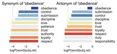
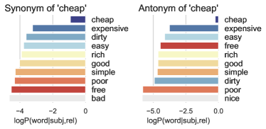
Figure 3 indicates illustrative examples in both of the opposite relations on the same subject words. Unexpectedly, there are words simultaneously predicted in the opposite relations. The quantitative results in Table 4 show that words with high probabilities of two opposite relations are common in many cases. The finding supports that the MNLMs may not clearly distinguish the subtle meaning of the opposite relations.

Furthermore, in order to demonstrate that such overlapping issue is undesirable and even problematic, we measure the ratio of incorrect answers by grading the predictions with answers from the opposite relation that can be regarded as wrong answers. Table 5 summarizes the result. Among the opposite relation pairs, the answer object of the ‘Synonym / Antonym’ pair is incompatible while the other opposite pairs can have identical answers. For example, there is an identical answer ‘pregnant’ for a given subject ‘person’ and the ‘Desire / NotDesire’ opposite relations. For this reason, we conduct the experiments on the ‘Synonym / Antonym’ pair. Hits@K, in this case, can be interpreted as the Miss@K, which is the ratio of predicted words definitely incorrect.

The experimental results demonstrate that MNLMs have a relatively high incorrect ratio considering it is unnecessary. In addition, as the size of the model and the training data increases, the performance of the models enhances. However, at the same time, the incorrect rate also increases generally. Thus, from these results, it is difficult for MNLMs to discern a precise difference between semantically related relationships specifically opposite relations. Additional examples of the overlapped predictions between the opposite relations can be found in Appendix F.

3.3 The Impact on the Masked Sentence Selection Procedure

3.4 The Impact of the Fine-tuning on the ConceptNet

4 Which Types of Questions Are Still Challenging for MNLMs?

We first classify the questions into the following six classes by referring to the question types of SQuAD [55]. :

• The synonymy class indicates the existence of a synonym relation between an answer sentence and a question.

• The commonsense knowledge class indicates that commonsense is required to solve a question.

• The no semantic variation class denotes that a question does neither belong to synonymy nor commonsense knowledge type.

• The multiple sentence reasoning class indicates that there are anaphora or clues scattered across multiple sentences.

• The typo class denotes a typographical error in a question or an answer sentence.

• The others class indicates that the presented answers are incorrectly tagged.

Then, we manually label the question types to see which types are more challenging than other types for the MNLM-based RC models.

The results show that there are obvious differences in the proportion of the question types between the correctly predicted questions and the incorrectly predicted questions. Across all models, the proportion of no semantic variation questions accounts for more than 50% in the correctly predicted questions, while the proportion decreases to about 30% in the incorrectly predicted questions. In other words, the easier questions have a higher proportion of the no semantic variation type questions. Likewise, the proportion of commonsense knowledge questions comprises approximately 22% to 25% in the correctly predicted questions, whereas the proportion increases to about 50% in incorrectly predicted questions.

From these results, we can infer that commonsense type questions can be substantially affected by the size of the pretrained corpus, that is, the size of knowledge contained in the corpus. Therefore, it is still challenging for the MNLM-based RC models to deal with questions with semantic variations, or questions that require commonsense knowledge to solve. This is an important discovery because it suggests that MNLMs should have the capacity to address commonsense knowledge, to overcome the limitations of MNLMs.

5 Main Results and a Possible Solution

Section 3 reveals that there are still limitations of the existing MNLMs even though they have the potential to infer commonsense knowledge. We conjecture that the existing MNLMs are heavily trained to learn observed information in the corpus and co-occurrences of the words rather than precise meanings of relations. Here, we first analyze observed joint frequencies of subject and object entities in the BERT pretrain data (English Wikipedia and Book Corpus). Subsequently, we discuss the impact of word frequency on knowledge probing results. Finally, we suggest a potential solution and a direction to handle the semantic variation type questions by utilizing an external commonsense repository.

5.1 Why MNLMs still Need External Commonsense Repository?

Figure 4: Statistics of the triples in the BERT pretrain datset. X-axis indicates the frequency with which subject and object entities are observed together. Y-axis is the number of triples for each section of the joint frequency of subject and object. The joint frequency and the proportion of triples for each frequency sector have a negative correlation.

(a) BERT_large

(b) ALBERT1_xlarge

Figure 5: The proportion of knowledge triples whose objects are in top 100 predictions for each model: (a) BERT_large, (b) ALBERT1_xlarge. X-axis indicates the frequency with which subject and object entities are observed together. Y-axis is the proportion of which the answer object can be found in top 100 model’s prediction for each frequency section. Blue bars indicate that the answer is in the top 100 predictions, while orange bars mean that the answer is not in the top 100 predictions. The results show that the joint frequency of subject and object affects the knowledge probing performance.

(a) BERT_large in top 100

(b) BERT_large in top k

(c) ALBERT1_xlarge in top 100

(d) ALBERT1_xlarge in top k

Figure 6:

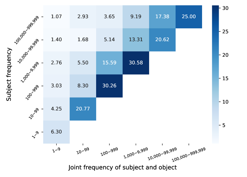
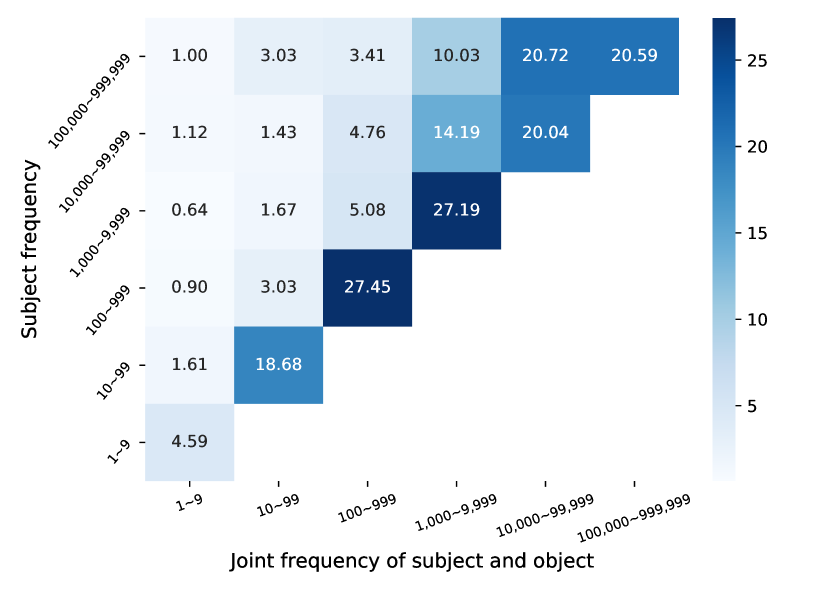
Herein, we analyze conditions for the MNLMs to learn the commonsense knowledge triples. Since there are no exclusive patterns for each relation, it is difficult to calculate the exact observation frequencies of the triples directly. Therefore, we adopt an assumption of the distant supervision paradigm of relation extraction tasks [56]. The assumption is that if sentences include a pair of entities that have a specific relation, then some of the sentences probably represent the relation of the entity pair. The more sentences contain the entity pair, the more sentences are likely to represent the relation.

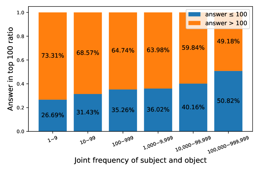
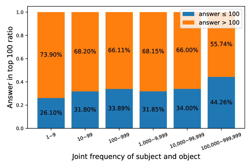
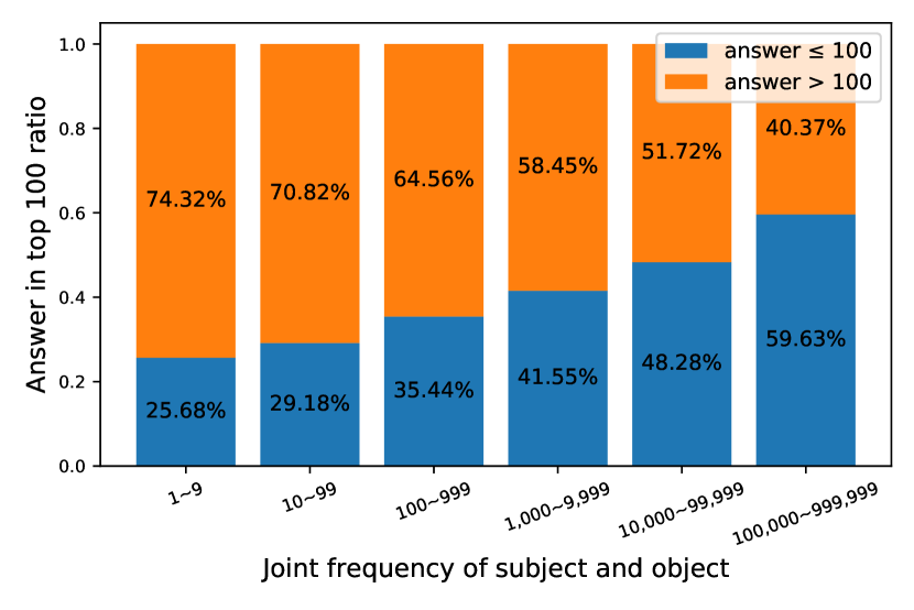
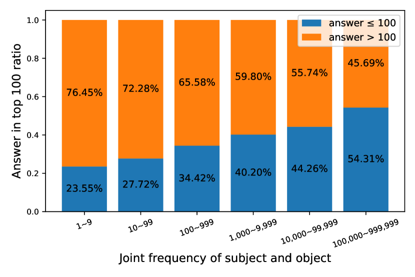
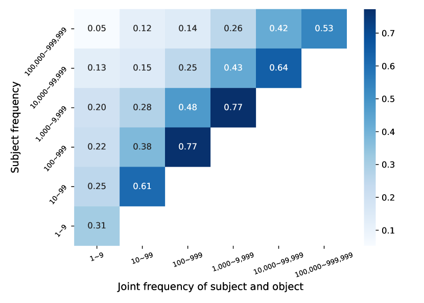
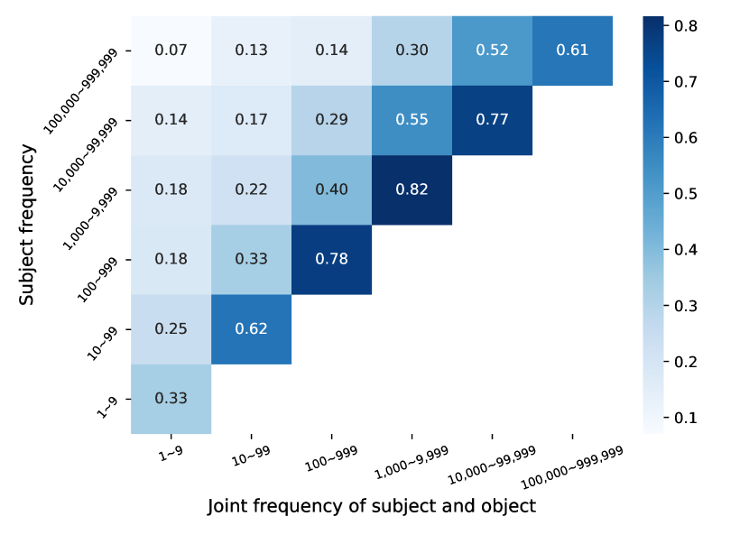
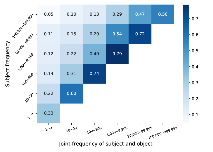
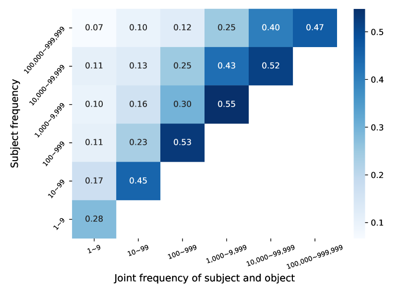
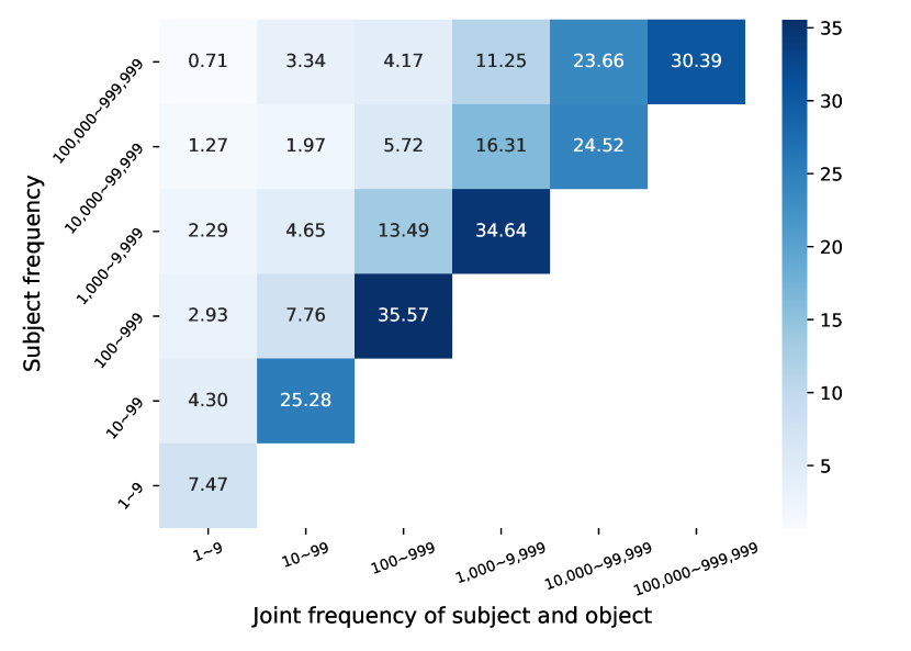
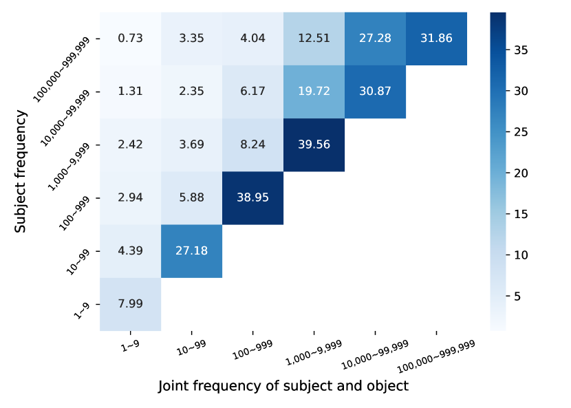
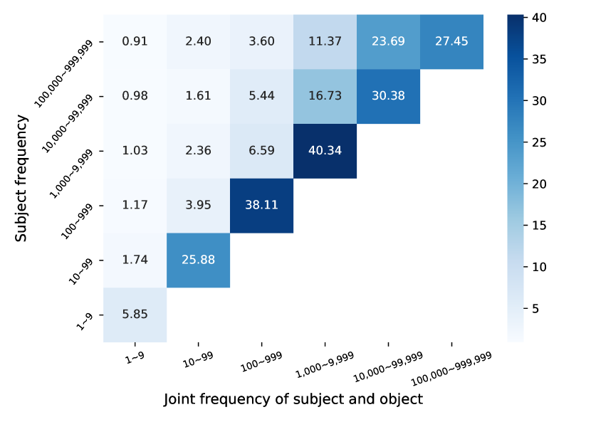
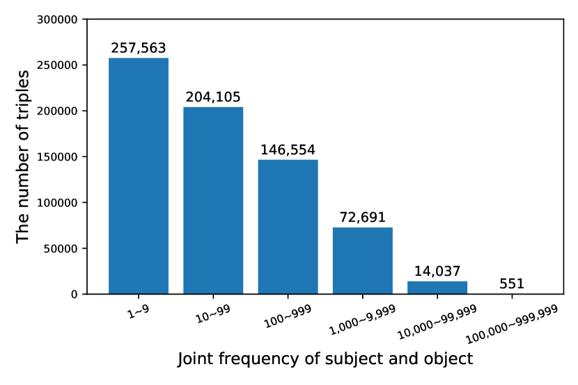
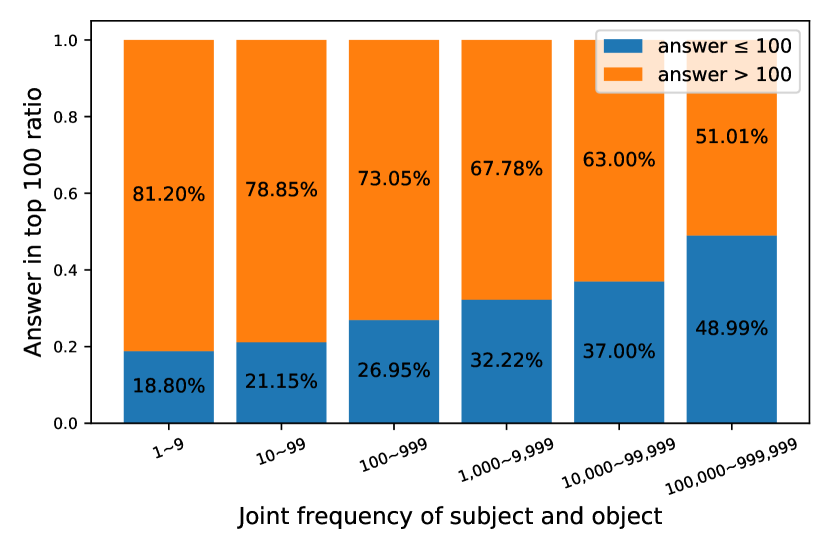
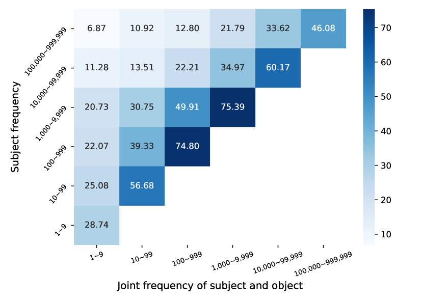
Figure 4 presents the statistics for the number of triples in each interval of the joint frequency of subject and object. Herein, many triples lack of the joint frequency. Then, we analyze the probing results of BERT and ALBERT1 models which are trained on the BERT pretrain dataset. Finally, we attest whether there is an answer object in the model’s top 100 or top k predictions based on the knowledge probing results of triples whose joint frequency of the subject and object entity pair is at least 1 time. In this section, we only show the results of the BERT_large and ALBERT1_xlarge models since the experimental results are consistent in the other models. Experimental results of the other models are demonstrated in Appendix J.

From these findings, training MNLMs on a larger dataset will be useful to enhance learning commonsense knowledge as the joint frequency of entity pairs is expected to increase in the larger dataset. However, it can be inefficient to simply increase the size of the dataset to sufficiently train relatively rare entity pairs. This is because, most entity pairs in the larger dataset can be redundant since the number of co-occurrences of word pairs follows the power-law distribution[57], similar to the well-known Zipf’s law[58]. Moreover, it does not guarantee that the conditional probability of entity pairs in the larger dataset will increase. Therefore, learning commonsense knowledge apart from the distribution of training corpora will be an important factor for overcoming the limitations of the existing MNLMs. Taking all these into consideration, it is still hard for the existing MNLMs to learn a significant portion of commonsense knowledge and may need help from external knowledge repositories or other tailored special purpose datasets.

5.2 Can An External Commonsense Repository Help for MNLMs to Solve the Questions including the Semantic Variation?

As discussed, it is clear that there are limitations in the existing MNLM-based RC models to infer semantic variation type questions. However, it is yet obscure whether the explicit complement of necessary knowledge can be a solution to the limitations of the MNLM-based RC models. Therefore, we conduct a controlled experiment to verify whether the external commonsense knowledge can help ameliorate the limitations. Specifically, we integrate adequate knowledge by enriching the text of a question or a context without additional training or changing the model.

Then, we evaluate our baseline models with the selected data in EM and F1 score of Equation (3), that is a harmonic mean of recall (Equation (2)) and precision (Equation (1)). We use BERT _large, ALBERT1 _xlarge, ALBERT2 _xlarge, and RoBERTa _large, as our baseline models. In addition, we conduct one-tailed t-test for the significant test.

$$\hskip 59.75095pt\text{Precision}=\frac{\text{\#\,of\,words\,in\,predicted\,answer\,matched\,with\,words\,in\,the\,ground\,truth}}{\text{\#\,of\,words\,in\,predicted\,answer}}$$ (1)

$$\hskip 66.86414pt\text{Recall}=\frac{\text{\#\,of\,words\,in\,predicted\,answer\,matched\,with\,words\,in\,the\,ground\,truth}}{\text{\#\,of\,words\,in\,the\,ground\,truth}}$$ (2)

$$\hskip 165.02606pt\text{F1}=\frac{2\times\text{Precision}\times\text{Recall}}{\text{Precision}+\text{Recall}}$$ (3)

6 Conclusion and Future Work

We investigate which types of commonsense knowledge are trained in the pretrained MNLMs by using the knowledge probing test. We find that MNLMs understand some commonsense knowledge while the trained knowledge is not precise enough to distinguish opposite relations. We also find that the questions requiring commonsense knowledge are still challenging to existing MNLM-based RC systems. Finally, we empirically demonstrate that the limitations of MNLMs can be complemented by integrating a commonsense knowledge repository. To the best of our knowledge, our study is the first to report the fundamental reason why existing MNLMs do not include a large portion of commonsense knowledge yet.

It is also a question to investigate how MNLMs learned to discern a subtle semantic difference between opposite relations from unlabeled text. Further, an automatic solution for the knowledge integrating remains to be developed as future work.

Acknowledgements
This work is supported by IITP grant funded by the Korea government (MIST) (2017-0-00255, Autonomous digital companion framework and application), IITP grant funded by the Korea government (MIST) (2017-0-01779, XAI), Artificial Intelligence Graduate School Program (KAIST) (2019-0-00075), and NAVER Corp.

Author contributions
S. Kwon, C. Kang, J. Han and J. Choi designed research. S. Kwon, C. Kang and J. Han performed research. S. Kwon, C. Kang and J. Choi analyzed the data. S. Kwon, J. Han and J. Choi revised the manuscript. S. Kwon, C. Kang, J. Han and J. Choi wrote the paper. S. Kwon, C. Kang, J. Han and J. Choi performed revision.

Data and code availability
All of data used in our manuscript are available in referred web link or in the supplementary information. The related codes are available in https://zenodo.org/record/3982680#.XzUvU6dxeUl

Competing interests
The authors declare no competing interests.

Table 1: Detail structures of MNLMs and NLMs

Model	Parameters	Layers	Hidden	Data
BERTbase	108M	12	768	16GB
BERTlarge	334M	24	1,024	16GB
ALBERT1base	12M	12	768	16GB
ALBERT1large	18M	24	1,024	16GB
ALBERT1xlarge	60M	24	2,048	16GB
ALBERT2base	12M	12	768	160GB
ALBERT2large	18M	24	1,024	160GB
ALBERT2xlarge	60M	24	2,048	160GB
RoBERTabase	108M	12	768	160GB
RoBERTalarge	334M	24	1,024	160GB
GPT1	119M	12	768	4GB
GPT2	1,558M	25	1,600	40GB
GPT3	175B	96	12,288	570GB

Table 2: Result of micro average and macro average performance of 1) the average hits@K performance of candidate masked sentences for each triple (‘AVG’) and 2) the hits@K of the selected masked sentence (‘SEL’).

Model	Sentence Selection	Hits@K
		Micro average			Macro average
		1	10	100	1	10	100
BERTbase	AVG	5.26	13.78	28.57	4.49	13.88	30.94
BERTlarge		5.00	13.94	28.60	5.27	15.15	32.64
BERTbase	SEL	7.39	19.07	36.24	6.33	18.19	37.39
BERTlarge		6.89	19.00	35.98	7.35	20.04	39.63

Table 3: Results of micro average and macro average hits@K for the ConceptNet relations.

Model	Hits@K
	Micro average			Macro average
	1	10	100	1	10	100
BERTbase	7.39$\pm$0.03	19.07$\pm$0.05	36.24$\pm$0.06	6.33$\pm$1.11	18.19$\pm$2.27	37.39$\pm$3.16
BERTlarge	6.89$\pm$0.03	19.00$\pm$0.05	35.98$\pm$0.06	7.35$\pm$1.21	20.04$\pm$2.30	39.63$\pm$3.23
ALBERT1base	8.36$\pm$0.04	19.21$\pm$0.05	36.33$\pm$0.06	3.58$\pm$0.64	13.51$\pm$1.33	30.82$\pm$2.05
ALBERT1large	5.46$\pm$0.03	15.55$\pm$0.05	32.04$\pm$0.06	3.62$\pm$0.60	11.91$\pm$1.22	30.45$\pm$1.65
ALBERT1xlarge	4.44$\pm$0.03	11.29$\pm$0.04	24.82$\pm$0.06	3.58$\pm$0.55	11.98$\pm$1.33	26.25$\pm$1.85
ALBERT2base	6.01$\pm$0.03	17.06$\pm$0.05	34.70$\pm$0.06	4.82$\pm$0.58	16.18$\pm$1.35	36.83$\pm$2.04
ALBERT2large	8.52$\pm$0.04	21.36$\pm$0.05	39.38$\pm$0.06	6.10$\pm$0.68	19.13$\pm$1.42	39.40$\pm$2.01
ALBERT2xlarge	8.83$\pm$0.04	21.93$\pm$0.05	39.23$\pm$0.06	7.29$\pm$0.90	21.32$\pm$1.67	41.73$\pm$1.92
RoBERTabase	2.95$\pm$0.02	10.26$\pm$0.04	26.71$\pm$0.06	4.53$\pm$0.72	14.13$\pm$1.53	32.94$\pm$2.25
RoBERTalarge	3.89$\pm$0.03	14.83$\pm$0.05	34.27$\pm$0.06	5.94$\pm$0.83	18.21$\pm$1.67	39.67$\pm$2.21
GPT1	0.30$\pm$0.01	3.75$\pm$0.02	15.82$\pm$0.05	0.98$\pm$0.30	6.85$\pm$1.07	24.79$\pm$2.12
GPT2	3.73$\pm$0.03	21.55$\pm$0.05	43.32$\pm$0.06	3.01$\pm$0.63	16.43$\pm$1.72	37.50$\pm$2.43
GPT3	3.58$\pm$0.02	24.07$\pm$0.06	52.13$\pm$0.06	3.69$\pm$0.78	18.89$\pm$1.97	44.81$\pm$2.52

• Data presented as mean $\pm$ standard error of mean

Table 4: Results of overlapping ratio at top K predictions between the opposite relations.

Relation	Model	Overlap@K*
		1	10	100
Synonym	BERTbase	45.21$\pm$0.99	44.19$\pm$0.66	47.77$\pm$0.61
	BERTlarge	37.00$\pm$0.96	41.12$\pm$0.62	46.09$\pm$0.56
	ALBERT1base	55.48$\pm$1.02	42.51$\pm$0.68	49.39$\pm$0.60
	ALBERT1large	46.26$\pm$1.03	38.82$\pm$0.69	46.74$\pm$0.60
	ALBERT1xlarge	35.03$\pm$0.98	34.22$\pm$0.66	40.97$\pm$0.61
	ALBERT2base	48.77$\pm$1.03	43.01$\pm$0.64	49.38$\pm$0.57
	ALBERT2large	62.24$\pm$1.00	55.99$\pm$0.48	61.08$\pm$0.37
	ALBERT2xlarge	52.13$\pm$1.03	52.90$\pm$0.55	57.66$\pm$0.45
	RoBERTabase	21.76$\pm$0.82	34.36$\pm$0.41	39.63$\pm$0.32
	RoBERTalarge	19.29$\pm$0.78	31.47$\pm$0.35	36.61$\pm$0.25
	GPT1	54.56$\pm$0.99	56.50$\pm$0.78	57.99$\pm$0.74
	GPT2	56.32$\pm$0.98	59.25$\pm$0.74	62.27$\pm$0.67
	GPT3	47.45$\pm$0.99	32.66$\pm$0.25	41.62$\pm$0.19
Desires	BERTbase	57.89$\pm$11.64	50.00$\pm$3.90	65.79$\pm$1.45
	BERTlarge	21.05$\pm$9.61	46.32$\pm$4.60	65.74$\pm$2.18
	ALBERT1base	78.95$\pm$9.61	72.63$\pm$3.96	72.79$\pm$1.14
	ALBERT1large	26.32$\pm$10.38	62.63$\pm$4.25	73.32$\pm$2.25
	ALBERT1xlarge	15.79$\pm$8.59	55.26$\pm$3.85	67.00$\pm$2.16
	ALBERT2base	31.58$\pm$10.96	58.95$\pm$3.66	69.37$\pm$1.58
	ALBERT2large	42.11$\pm$11.64	60.53$\pm$3.63	69.63$\pm$1.92
	ALBERT2xlarge	57.89$\pm$11.64	58.42$\pm$4.73	71.42$\pm$2.30
	RoBERTabase	52.63$\pm$11.77	48.95$\pm$3.74	61.79$\pm$2.16
	RoBERTalarge	5.26$\pm$5.26	41.58$\pm$4.41	58.26$\pm$1.94
	GPT1	52.63$\pm$11.77	58.42$\pm$3.18	62.84$\pm$1.37
	GPT2	57.89$\pm$11.64	58.95$\pm$3.23	64.89$\pm$1.64
	GPT3	42.11$\pm$11.64	45.79$\pm$3.36	54.05$\pm$2.29
HasProperty	BERTbase	20.93$\pm$6.28	26.74$\pm$2.70	37.05$\pm$2.55
	BERTlarge	23.26$\pm$6.52	20.47$\pm$2.82	31.93$\pm$2.71
	ALBERT1base	16.67$\pm$5.82	35.00$\pm$3.53	49.40$\pm$2.72
	ALBERT1large	14.29$\pm$5.46	30.00$\pm$3.25	41.33$\pm$2.89
	ALBERT1xlarge	9.52$\pm$4.58	19.76$\pm$3.43	33.69$\pm$2.94
	ALBERT2base	19.05$\pm$6.13	25.48$\pm$3.72	33.38$\pm$3.38
	ALBERT2large	19.05$\pm$6.13	26.43$\pm$3.88	34.19$\pm$3.57
	ALBERT2xlarge	14.29$\pm$5.46	20.71$\pm$3.33	30.07$\pm$3.10
	RoBERTabase	11.63$\pm$4.95	14.88$\pm$2.69	23.91$\pm$2.71
	RoBERTalarge	4.65$\pm$3.25	11.40$\pm$1.99	23.14$\pm$2.66
	GPT1	25.58$\pm$6.73	30.93$\pm$2.84	38.84$\pm$2.42
	GPT2	30.23$\pm$7.09	31.40$\pm$2.61	37.67$\pm$2.44
	GPT3	27.91$\pm$6.92	30.00$\pm$2.53	35.72$\pm$2.27
CapableOf	BERTbase	0.00$\pm$0.00	62.00$\pm$8.60	69.80$\pm$3.25
	BERTlarge	40.00$\pm$24.49	56.00$\pm$5.10	73.60$\pm$2.54
	ALBERT1base	40.00$\pm$24.49	46.00$\pm$5.10	60.80$\pm$5.46
	ALBERT1large	0.00$\pm$0.00	50.00$\pm$10.00	70.40$\pm$3.20
	ALBERT1xlarge	80.00$\pm$20.00	54.00$\pm$5.10	60.80$\pm$2.24
	ALBERT2base	40.00$\pm$24.49	50.00$\pm$7.75	67.40$\pm$1.63
	ALBERT2large	20.00$\pm$20.00	32.00$\pm$8.00	52.40$\pm$2.25
	ALBERT2xlarge	20.00$\pm$20.00	50.00$\pm$5.48	68.20$\pm$2.35
	RoBERTabase	20.00$\pm$20.00	44.00$\pm$6.00	55.40$\pm$3.59
	RoBERTalarge	40.00$\pm$24.49	36.00$\pm$7.48	55.80$\pm$2.40
	GPT1	20.00$\pm$20.00	36.00$\pm$8.72	61.40$\pm$2.38
	GPT2	20.00$\pm$20.00	36.00$\pm$9.27	60.20$\pm$2.35
	GPT3	20.00$\pm$20.00	28.00$\pm$5.83	52.20$\pm$1.46

• Data presented as mean $\pm$ standard error of mean

• Overlap@K = The ratio of overlapping words in top K predictions for two opposite relations.

Table 5: Results of missed prediction ratio at top K predictions between the opposite relations.

Model	Miss@K*
	Synonym / Antonym			Antonym / Synonym
	1	10	100	1	10	100
BERTbase	9.40$\pm$0.50	29.12$\pm$0.77	50.91$\pm$0.84	7.02$\pm$0.41	17.64$\pm$0.59	32.16$\pm$0.74
BERTlarge	12.89$\pm$0.57	32.24$\pm$0.79	53.48$\pm$0.84	4.95$\pm$0.34	17.51$\pm$0.61	31.63$\pm$0.75
ALBERT1base	1.76$\pm$0.24	18.78$\pm$0.68	38.46$\pm$0.84	9.77$\pm$0.46	16.93$\pm$0.58	29.64$\pm$0.71
ALBERT1large	3.72$\pm$0.33	19.42$\pm$0.68	39.95$\pm$0.85	7.43$\pm$0.41	14.83$\pm$0.55	26.45$\pm$0.69
ALBERT1xlarge	9.50$\pm$0.51	26.32$\pm$0.76	45.97$\pm$0.86	5.55$\pm$0.37	13.52$\pm$0.53	27.23$\pm$0.70
ALBERT2base	6.45$\pm$0.42	24.34$\pm$0.75	43.35$\pm$0.86	8.72$\pm$0.44	17.57$\pm$0.60	31.93$\pm$0.74
ALBERT2large	9.69$\pm$0.52	29.42$\pm$0.79	51.51$\pm$0.86	8.10$\pm$0.43	23.09$\pm$0.67	40.16$\pm$0.76
ALBERT2xlarge	12.72$\pm$0.58	33.34$\pm$0.82	54.71$\pm$0.85	8.34$\pm$0.44	23.39$\pm$0.67	40.66$\pm$0.78
RoBERTabase	2.90$\pm$0.29	12.24$\pm$0.55	28.34$\pm$0.76	1.33$\pm$0.18	10.34$\pm$0.48	27.74$\pm$0.69
RoBERTalarge	10.48$\pm$0.53	30.85$\pm$0.80	52.75$\pm$0.86	10.56$\pm$0.48	23.25$\pm$0.67	39.78$\pm$0.77
GPT1	2.88$\pm$0.27	13.03$\pm$0.56	32.29$\pm$0.80	5.02$\pm$0.34	16.57$\pm$0.57	31.77$\pm$0.72
GPT2	5.56$\pm$0.38	18.02$\pm$0.65	39.11$\pm$0.84	2.73$\pm$0.26	17.83$\pm$0.61	38.34$\pm$0.75
GPT3	3.06$\pm$0.30	18.91$\pm$0.80	52.98$\pm$1.22	0.24$\pm$0.08	6.45$\pm$0.43	39.02$\pm$1.00

• Data presented as mean $\pm$ standard error of mean

• Miss@K = The ratio of words that are considered right when graded with the opposite relation (undesirable) in top K predictions.

Table 6: Comparison of macro average hits@K on pretrained and fune-tuned BERT models. Herin, Avg. indicates average.

Train Status	Model	Avg. Type	Hits@K
			1				10				100
			Fold 0	Fold 1	Fold 2	Avg.*	Fold 0	Fold 1	Fold 2	Avg.	Fold 0	Fold 1	Fold 2	Avg.
Pretrained	BERTbase	Micro	6.67	5.05	6.19	5.97	17.72	16.31	17.38	17.14	36.13	33.78	34.80	34.90
		Macro	7.93	7.74	7.79	7.82	19.69	19.65	19.62	19.65	37.29	37.25	37.21	37.25
	BERTlarge	Micro	8.00	5.51	7.31	6.94	20.03	17.65	18.27	18.65	38.17	36.31	36.07	36.85
		Macro	7.27	7.16	7.24	7.22	19.31	19.27	19.19	19.26	37.09	36.90	36.88	36.96
Fine-tuned	BERTbase	Micro	17.73	16.40	16.25	16.79	42.52	40.67	40.39	41.19	66.87	62.82	63.80	64.50
		Macro	29.58	29.60	29.77	29.65	52.20	52.22	52.16	52.19	70.88	70.97	70.89	70.91
	BERTlarge	Micro	21.39	19.14	19.55	20.03	46.93	43.63	43.93	44.83	72.23	68.20	70.23	70.22
		Macro	32.41	32.35	32.53	32.43	55.86	55.79	55.96	55.87	74.28	74.26	74.23	74.26

• Average of the performances of Fold 1, 2 and 3

Table 7: Results of overlapping ratio at top K predictions of fine-tuned BERT models between the opposite relations. Herein, ‘-’ indicates when it is impossible to evaluate overlap@K since there is no example of an opposite relation for all subject-relation pairs in the same test fold.

		Overlap@K*
		1			10			100
Relation	Model	Fold 0	Fold 1	Fold 2	Fold 0	Fold 1	Fold 2	Fold 0	Fold 1	Fold 2
Desires	BERTbase	0.00	100.00	50.00	55.00	60.00	50.00	63.50	72.50	67.50
	BERTlarge	100.00	100.00	50.00	75.00	75.00	60.00	62.50	68.00	64.50
HasProperty	BERTbase	100.00	20.00	0.00	60.00	38.00	40.00	43.00	52.00	45.67
	BERTlarge	0.00	40.00	0.00	30.00	20.00	30.00	32.00	41.60	45.67
CapableOf	BERTbase	-	100.00	-	-	60.00	-	-	78.00	-
	BERTlarge	-	100.00	-	-	70.00	-	-	76.00	-
Synonym	BERTbase	78.82	80.00	70.59	69.88	66.94	68.37	71.32	70.59	70.17
	BERTlarge	47.06	54.44	44.94	51.47	50.28	49.55	56.16	56.76	55.16

• Overlap@K = The ratio of overlapping words in top K predictions for two opposite relations.

Table 8: Results of missed prediction ratio at top K predictions of fine-tuned BERT models between the opposite relations.

		Miss@K*
		1			10			100
Model		Fold 0	Fold 1	Fold 2	Fold 0	Fold 1	Fold 2	Fold 0	Fold 1	Fold 2
	BERTbase	3.33	2.89	3.87	29.57	28.48	31.22	57.35	57.50	54.98
Synonym / Antonym	BERTlarge	4.42	4.21	4.36	29.53	29.63	30.35	56.34	58.43	58.21
	BERTbase	17.16	13.63	13.63	37.56	35.20	35.24	58.91	56.75	57.78
Antonym / Synonym	BERTlarge	8.69	8.57	8.20	31.50	27.40	28.24	55.26	49.87	52.70

• Miss@K = The ratio of words that are considered right when graded with the opposite relation (undesirable) in top K predictions.

Table 9: Total proportion of has answer questions with less lexical overlapping (similarity < 0.2) and proportions of question types for each model in SQuAD.

Model	Status*	Question type						Number of examples
		Semantic variation		Multiple sentence reasoning	No semantic variation	Typo	Others
		Synonymy	Commonsense Knowledge
BERTlarge	Correct	27.29	22.54	11.82	54.14	1.22	1.10	905
BERTlarge	Incorrect	30.71	49.46	19.84	27.45	1.63	2.99	368
ALBERT1xlarge	Correct	28.06	24.40	12.46	51.52	1.15	1.15	955
ALBERT1xlarge	Incorrect	28.93	48.11	19.18	31.13	1.89	3.14	318
ALBERT2xlarge	Correct	28.22	24.41	12.56	51.80	1.13	0.93	971
ALBERT2xlarge	Incorrect	28.48	49.34	19.21	29.14	1.99	3.97	302
RoBERTalarge	Correct	28.81	25.12	12.36	50.55	1.30	1.10	1003
RoBERTalarge	Incorrect	26.30	49.63	20.74	31.11	1.48	3.70	270
Overall†	Correct	27.29	17.86	10.97	57.81	1.27	0.84	711
Overall	Incorrect	25.69	55.96	22.02	24.77	1.83	4.59	109
Total proportion		28.28	30.32	14.14	46.43	1.34	1.65	1273

• The categories can be tagged with duplicates except for semantic variation and no semantic variation.

• Correct: Questions correctly predicted by the model, Incorrect: Questions incorrectly predicted by the model

• Questions succeed or failed to predict by all experimental models commonly

Table 10: Total proportion of question types for each model in ReCORD.

Model	Status*	Question type						Number of examples
		Semantic variation		Multiple sentence reasoning	No semantic variation	Typo	Others
		Synonymy	Commonsense Knowledge
BERTlarge	Correct	13.38	88.73	13.38	1.41	0.00	4.23	142
BERTlarge	Incorrect	17.24	72.41	6.90	3.45	3.45	15.52	58
ALBERT1xlarge	Correct	13.70	88.36	13.01	1.37	0.68	3.42	146
ALBERT1xlarge	Incorrect	16.67	72.22	7.41	3.70	1.85	18.52	54
ALBERT2xlarge	Correct	12.58	88.74	12.58	1.32	1.32	3.31	151
ALBERT2xlarge	Incorrect	20.41	69.39	8.16	4.08	0.00	20.41	49
RoBERTalarge	Correct	11.84	91.45	12.50	1.32	0.66	1.97	152
RoBERTalarge	Incorrect	22.92	60.42	8.33	4.17	2.08	25.00	48
Overall†	Correct	11.82	90.91	14.55	1.82	0.00	1.82	110
Overall	Incorrect	11.82	42.11	5.26	10.53	0.00	42.11	19
Total proportion		14.50	84.00	11.50	2.00	1.00	7.50	200

• The categories can be tagged with duplicates except for semantic variation and no semantic variation.

• Correct: Questions correctly predicted by the model, Incorrect: Questions incorrectly predicted by the model

• Questions succeed or failed to predict by all experimental models commonly

Table 11: Examples of manual external commonsense knowledge integration in SQuAD.

Required Knowledge*	Question	Context
uv Synonym ultraviolet radiation	_____ Helps the biospher from UV, which is the same as ultraviolet radiation.	… the high-altitude ozone layer helps protect the biosphere from ultraviolet radiation, …
rare Antonym frequent	How frequent is snow in the Southwest of the state?	… But snow is very rare, which is the opposite of frequent, in the Southwest of the state, …
punishment RelatedTo sentence	Why would one want to give more punishment, which is related to sentence?	… the judge increased her sentence from 40 to 60 days. …

• The blue words indicate the subject term of the triple
  The red words indicate the relation or the relation’s relative pronoun template of the triple
  The turquoise words indicate the object term of the triple
  

Table 12: Examples of manual external commonsense knowledge integration in ReCoRD.

Required Knowledge*	Question	Context
uv Synonym ultraviolet radiation	_____ Helps the biospher from UV	… the high-altitude ozone layer helps protect the biosphere from ultraviolet radiation, … @highlight uv is the same as ultraviolet radiation.
rare Antonym frequent	How frequent is snow in the Southwest of the state?	… But snow is very rare in the Southwest of the state, … @highlight rare is the opposite of frequent
punishment RelatedTo sentence	Why would one want to give more punishment?	… the judge increased her sentence from 40 to 60 days. …@highlight punishment is related to sentence

• The blue words indicate the subject term of the triple
  The red words indicate the relation or the relation’s relative pronoun template of the triple
  The turquoise words indicate the object term of the triple
  

Table 13: Experimental results of the knowledge integration test.

Dataset	Model	Status	Original text		Knowledge integrated text		$\Delta$ F1
			EM*	F1†	EM	F1
SQuAD	BERTlarge	Correct	100.00	100.00	93.37	95.93	-4.07
		Incorrect	0.00	28.08	11.53	37.11	9.53
	ALBERT1xlarge	Correct	100.00	100.00	87.22	89.73	-10.27
		Incorrect	0.00	29.86	18.75	46.64	16.78
	ALBERT2xlarge	Correct	100.00	100.00	85.71	90.59	-9.41
		Incorrect	0.00	29.86	14.49	44.37	13.02
	RoBERTalarge	Correct	100.00	100.00	90.00	93.48	-6.52
		Incorrect	0.00	32.94	14.06	43.43	10.49
ReCORD	BERTlarge	Correct	100.00	100.00	98.68	98.68	-1.32
		Incorrect	0.00	2.81	10.71	10.71	7.90
	ALBERT1xlarge	Correct	100.00	100.00	97.40	97.40	-2.60
		Incorrect	0.00	11.77	14.81	27.04	15.27
	ALBERT2xlarge	Correct	100.00	100.00	98.77	98.77	-1.23
		Incorrect	0.00	15.51	8.70	21.96	6.45
	RoBERTalarge	Correct	100.00	100.00	98.72	98.72	-1.28
		Incorrect	0.00	19.55	3.85	23.40	3.85

• F1 score

• Exact match score

Appendix A Details on the Templates

Table 1: This table presents details on the templates of the relations in the ConceptNet used in the experiments. Note that, difference from BERT, ALBERT and RoBERTa models, only original templates where [[OBJ]] comes at the end of the sentence are utilized for GPT models because of the characteristics of GPT models that decode input sentences from left to right.

Relation	Original Templates	# of samples	# of average answers
RelatedTo	‘[[SUBJ]] is related to [[OBJ]] .’; ‘[[SUBJ]] is like [[OBJ]] .’; ‘[[SUBJ]] is associated to [[OBJ]] .’	252,003	2.85
HasContext	‘[[SUBJ]] is used in the context of [[OBJ]] .’; ‘[[SUBJ]] is a kind of [[OBJ]] .’; ‘[[SUBJ]] is a type of [[OBJ]] .’	84,755	1.22
IsA	‘[[SUBJ]] is a [[OBJ]] .’; ‘[[SUBJ]] is used in the region of [[OBJ]] .’; ‘[[SUBJ]] is utilized in [[OBJ]] .’	67,208	1.22
DerivedFrom	‘[[SUBJ]] is derived from [[OBJ]] .’; ‘[[SUBJ]] is stemmed from [[OBJ]] .’; ‘[[SUBJ]] is originated from [[OBJ]] .’	52,297	1.05
Synonym	‘[[SUBJ]] is same with [[OBJ]] .’; ‘[[SUBJ]] is same as [[OBJ]] .’; ‘[[SUBJ]] and [[OBJ]] are the same .’; ‘[[SUBJ]] and [[OBJ]] are the synonym .’	20,065	1.64
FormOf	‘[[OBJ]] is the root word of [[SUBJ]] .’; ‘[[SUBJ]] is come from [[OBJ]] .’; ‘[[SUBJ]] is originated from [[OBJ]] .’	18,405	1.01
SimilarTo	‘[[SUBJ]] is similar to [[OBJ]] .’; ‘[[SUBJ]] is like to [[OBJ]] .’; ‘[[SUBJ]] are comparable to [[OBJ]]’	7,266	1.35
EtymologicallyRelatedTo	‘[[SUBJ]] is etymologically related to [[OBJ]] .’; ‘[[SUBJ]] is etymologically like [[OBJ]] .’; ‘[[SUBJ]] is etymologically associated to [[OBJ]] .’	7,081	1.27
AtLocation	‘Something you find at [[OBJ]] is [[SUBJ]] .’; ‘you are likely to find [[OBJ]] in [[SUBJ]] .’; ‘[[[OBJ]] is located in [[SUBJ]] .	6,532	1.95
MannerOf	‘[[SUBJ]] is a way to [[OBJ]] .’; ‘[[SUBJ]] is a manner to [[OBJ]] .’; ‘[[SUBJ]] is a means to [[OBJ]] .’	5,963	1.56
Antonym	‘[[SUBJ]] and [[OBJ]] are opposite .’; ‘[[SUBJ]] is the opposite of [[OBJ]] .’; ‘[[SUBJ]] and [[OBJ]] are antonym .’	3,457	1.98
HasProperty	‘[[SUBJ]] can be [[OBJ]] .’; ‘[[SUBJ]] is [[OBJ]] .’; ‘[[SUBJ]] has [[OBJ]] .’	2,708	1.25
PartOf	‘[[SUBJ]] is part of [[OBJ]] .’; ‘[[OBJ]] is part of [[SUBJ]] .’; ‘[[SUBJ]] has [[OBJ]] .’; ‘[[SUBJ]] contains [[OBJ]] .’	2,317	1.22
UsedFor	‘[[SUBJ]] may be used for [[OBJ]] .’; ‘[[SUBJ]] is used for [[OBJ]] .’; ‘[[SUBJ]] is for [[OBJ]] .’	2,090	3.01
DistinctFrom	‘[[SUBJ]] is not [[OBJ]] .’; ‘[[SUBJ]] is different from [[OBJ]] .’; ‘[[SUBJ]] is distinct from [[OBJ]] .’	1,184	2.08
HasPrerequisite	‘[[SUBJ]] requires [[OBJ]] .’; ‘Something you need to do before you [[SUBJ]] is [[OBJ]] .’; ‘If you want to [[SUBJ]] then you should [[OBJ]] .’	1,127	3.06
HasSubevent	‘One of the things you do when you [[SUBJ]] is [[OBJ]] .’; ‘Something you might do while [[SUBJ]] is [[OBJ]] .’	1,100	3.10
Causes	‘[[SUBJ]] causes [[OBJ]] .’; ‘The effect of [[SUBJ]] is that [[OBJ]] .’; ‘Something that might happen as a consequence of [[SUBJ]] is [[OBJ]] .’	952	3.68
HasA	‘[[SUBJ]] contains [[OBJ]] .’; ‘[[SUBJ]] has [[OBJ]] .’; ‘[[SUBJ]] includes [[OBJ]] .’	847	1.3
InstanceOf	‘[[SUBJ]] is an instance of [[OBJ]] .’; ‘[[SUBJ]] is an example of [[OBJ]] .’; ‘[[SUBJ]] is an illustration of [[OBJ]] .’	738	1.03
CapableOf	‘[[SUBJ]] can [[OBJ]] .’; ‘[[SUBJ]] may [[OBJ]] .’; ‘[[SUBJ]] sometimes [[OBJ]] .’	656	1.40
MotivatedByGoal	‘You would [[OBJ]] because you want to [[SUBJ]] .’; ‘You would [[OBJ]] because you like to [[SUBJ]] .’; ‘If you want to [[SUBJ]] then you should [[OBJ]] .’	593	2.78
MadeOf	‘[[SUBJ]] can be made of [[OBJ]] .’; ‘[[SUBJ]] is made from [[OBJ]] .’; ‘[[SUBJ]] consists of [[OBJ]] .’	303	1.16
Entails	‘[[SUBJ]] entails [[OBJ]] .’; ‘[[SUBJ]] brings about [[OBJ]] .’; ‘[[SUBJ]] leads to [[OBJ]] .’	284	1.06
Desires	‘[[SUBJ]] wants [[OBJ]] .’; ‘[[SUBJ]] likes to [[OBJ]] .’; ‘[[SUBJ]] desires to [[OBJ]] .’	196	2.62
NotHasProperty	‘[[SUBJ]] can not be [[OBJ]] .’; ‘[[SUBJ]] does not have [[OBJ]] .’; ‘[[SUBJ]] is not [[OBJ]] .’	158	1.08
CreatedBy	‘[[SUBJ]] is created by [[OBJ]] .’; ‘[[SUBJ]] is developed by [[OBJ]] .’; ‘[[SUBJ]] is invented by [[OBJ]] .’	102	1.22
NotDesires	‘[[SUBJ]] does not want [[OBJ]] .’; ‘[[SUBJ]] does not want to [[OBJ]] .’; ‘[[SUBJ]] dislikes to [[OBJ]] .’	70	4.4
DefinedAs	[[SUBJ]] can be defined as [[OBJ]] ; ‘[[SUBJ]] is the [[OBJ]] .’; ‘The definition of [[SUBJ]] is [[OBJ]] .’	63	1.14
NotCapableOf	‘[[SUBJ]] cannot [[OBJ]] .’; ‘[[SUBJ]] does not [[OBJ]] .’; ‘[[SUBJ]] may not [[OBJ]] .’	42	1.1
LocatedNear	‘[[SUBJ]] is typically near [[OBJ]] .’; ‘[[SUBJ]] is typically close by [[OBJ]] .’; ‘[[SUBJ]] is typically nearby [[OBJ]] .”	32	1.03
EtymologicallyDerivedFrom	‘[[SUBJ]] is etymologically derived from [[OBJ]] .’; ‘[[SUBJ]] is etymologically stemmed from [[OBJ]] .’; ‘[[SUBJ]] is etymologically originated from [[OBJ]] .’	23	1

Appendix B Details on the Grammar Transformation

Since injecting a subject and a object directly into a template can induce a grammatically problematic sentence, we apply ensuing regulations yielding candidate sentences. Then, by using a language model, we choose the most grammatical sentence among the grammatically diversified sentences.

1. If the first word is a adjective or noun, or if the first word is a verb and the second word is a noun or adjective, prepend a definite or indefinite article. (i.e. opera -> an opera, the opera)

2. If the first word is infinitive verb, then convert it to a gerund. (i.e. make -> making)

3. If first word is number, then pluralize the next word. (i.e. two leg -> two legs)

4. Adding variations of plural verb if it is possible, to keep subject-verb concord. (i.e. skywards is -> skywards are)

In order to analyze the part-of-speech tags, python library spaCy (https://spacy.io) is applied. Furthermore, pattern (https://github.com/clips/pattern/wiki) is used for conjugation and pluralization. Finally, GPT model (https://huggingface.co/transformers/model_doc/gpt.html) is utilized to figure out which candidate sentence is most likely to be grammatically.

Appendix C Qualitative Results of Knowledge Probing Test

(e)
(f)
(g)

Figure 1: Representative probabilistic distributions of the knowledge probing test results on the BERT_base model. (a), (b) and (c) respectively show results of ‘antonym of sound’, ‘antonym of spring’ and ‘antonym of larboard’. The y-axis indicates log₁₀ probability and the x-axis denotes the ranking of the words. Correct answers are marked in red.

Figure 1 visualizes three sampled examples of the knowledge probing test results. We demonstrate predicted conditional log likelihood results of Equation (1) of the examples.

$$\hskip 85.35826pt\text{Conditional\,log\,likelihood\,=\,}logP\text{(word|subject,relation)}$$ (1)

First, we can see that the ‘antonym of spring’ case not only are the correct answers ranked high, but they show a significantly higher likelihood compared to non-answers. We suppose that the semantic triple of this case is relatively frequently trained on some words as the model is significantly more confident in some words than others. On the other hand, the ‘antonym of sound’ case answers are predicted, but there is a non-answer that has a higher rank than the answers and there is little difference between answers and non-answers likelihoods. Finally, in the ‘antonym of larboard’ case, all answers are failed to be predicted and all candidates have similar likelihoods. We conjecture that the relations are not trained enough in the training as the model is not as confident on any of its predictions.

Appendix D Quantitative Analysis for Probabilistic Distributions

Table 2: Results of the BERT $hits@K$ metric for each relation in ConceptNet.

Relations	$hits@K$
	BERTbase			BERTlarge
	1	10	100	1	10	100
RelatedTo	3.20$\pm$0.03	9.49$\pm$0.05	22.68$\pm$0.07	2.95$\pm$0.03	9.15$\pm$0.05	21.89$\pm$0.07
HasContext	7.05$\pm$0.09	24.33$\pm$0.15	48.07$\pm$0.17	7.11$\pm$0.09	24.17$\pm$0.15	47.68$\pm$0.17
IsA	22.90$\pm$0.16	42.06$\pm$0.18	62.76$\pm$0.18	22.32$\pm$0.16	42.51$\pm$0.19	63.06$\pm$0.18
DerivedFrom	13.16$\pm$0.15	32.03$\pm$0.20	52.81$\pm$0.22	9.27$\pm$0.13	27.74$\pm$0.20	49.74$\pm$0.22
Synonym	9.58$\pm$0.20	27.81$\pm$0.30	47.95$\pm$0.33	8.46$\pm$0.19	27.69$\pm$0.30	48.62$\pm$0.33
FormOf	0.26$\pm$0.04	15.73$\pm$0.26	31.19$\pm$0.32	0.98$\pm$0.07	24.05$\pm$0.30	36.07$\pm$0.34
EtymologicallyRelatedTo	6.91$\pm$0.28	14.98$\pm$0.41	26.00$\pm$0.51	7.67$\pm$0.30	18.43$\pm$0.44	32.07$\pm$0.54
SimilarTo	1.03$\pm$0.12	4.62$\pm$0.24	13.11$\pm$0.39	1.94$\pm$0.16	8.86$\pm$0.33	21.33$\pm$0.47
AtLocation	0.03$\pm$0.02	1.21$\pm$0.13	13.09$\pm$0.38	0.00$\pm$0.00	0.59$\pm$0.09	9.30$\pm$0.33
MannerOf	2.05$\pm$0.18	9.68$\pm$0.36	38.37$\pm$0.57	2.04$\pm$0.18	10.08$\pm$0.37	38.00$\pm$0.58
PartOf	0.00$\pm$0.00	6.19$\pm$0.50	26.56$\pm$0.90	0.00$\pm$0.00	7.00$\pm$0.53	26.30$\pm$0.90
Antonym	7.49$\pm$0.41	21.38$\pm$0.63	38.39$\pm$0.76	10.43$\pm$0.48	25.61$\pm$0.68	43.11$\pm$0.78
HasProperty	4.81$\pm$0.40	18.56$\pm$0.73	47.18$\pm$0.95	7.01$\pm$0.48	25.44$\pm$0.82	52.75$\pm$0.94
UsedFor	5.51$\pm$0.41	21.57$\pm$0.72	48.30$\pm$0.86	6.42$\pm$0.46	20.44$\pm$0.71	48.43$\pm$0.87
DistinctFrom	5.69$\pm$0.58	23.69$\pm$1.11	47.43$\pm$1.30	9.48$\pm$0.76	28.55$\pm$1.17	53.26$\pm$1.29
HasPrerequisite	0.13$\pm$0.10	0.28$\pm$0.14	8.01$\pm$0.66	0.13$\pm$0.10	0.41$\pm$0.15	9.16$\pm$0.67
HasSubevent	5.21$\pm$0.53	17.90$\pm$0.89	47.49$\pm$1.14	6.32$\pm$0.58	20.55$\pm$0.92	50.75$\pm$1.12
Causes	0.12$\pm$0.11	0.77$\pm$0.26	8.47$\pm$0.80	0.53$\pm$0.23	0.99$\pm$0.30	5.08$\pm$0.62
HasA	5.93$\pm$0.79	17.27$\pm$1.28	44.98$\pm$1.67	7.81$\pm$0.91	22.88$\pm$1.42	52.11$\pm$1.68
InstanceOf	0.17$\pm$0.17	7.93$\pm$1.12	27.10$\pm$1.84	0.00$\pm$0.00	7.93$\pm$1.12	34.77$\pm$1.97
CapableOf	9.66$\pm$1.12	26.69$\pm$1.67	56.86$\pm$1.87	11.96$\pm$1.23	30.66$\pm$1.74	57.30$\pm$1.86
MotivatedByGoal	2.62$\pm$0.51	6.77$\pm$0.74	24.93$\pm$1.32	1.40$\pm$0.37	5.92$\pm$0.71	25.29$\pm$1.31
MadeOf	18.32$\pm$2.20	53.01$\pm$2.85	74.23$\pm$2.49	19.74$\pm$2.27	51.02$\pm$2.85	74.57$\pm$2.49
Entails	0.71$\pm$0.50	3.90$\pm$1.15	16.08$\pm$2.16	1.77$\pm$0.79	3.90$\pm$1.15	13.77$\pm$2.04
Desires	7.34$\pm$1.85	18.29$\pm$2.68	33.43$\pm$3.30	7.79$\pm$1.91	18.94$\pm$2.71	34.01$\pm$3.31
NotHasProperty	2.55$\pm$1.26	16.24$\pm$2.94	35.88$\pm$3.77	6.37$\pm$1.96	23.46$\pm$3.36	48.83$\pm$3.94
CreatedBy	6.38$\pm$2.42	20.04$\pm$3.88	47.25$\pm$5.05	4.79$\pm$2.15	22.16$\pm$4.18	47.34$\pm$4.99
DefinedAs	12.22$\pm$4.19	25.28$\pm$5.54	50.56$\pm$6.36	16.67$\pm$4.85	37.50$\pm$6.15	55.00$\pm$6.38
NotDesires	9.60$\pm$3.46	13.95$\pm$4.11	23.60$\pm$5.00	9.60$\pm$3.46	13.95$\pm$4.11	25.05$\pm$5.11
NotCapableOf	23.17$\pm$6.56	48.78$\pm$7.90	73.78$\pm$6.87	28.05$\pm$6.99	46.34$\pm$7.88	79.88$\pm$6.25
LocatedNear	0.00$\pm$0.00	18.75$\pm$7.01	46.88$\pm$8.96	3.12$\pm$3.12	12.50$\pm$5.94	37.50$\pm$8.70
EtymologicallyDerivedFrom	8.70$\pm$6.01	13.04$\pm$7.18	13.04$\pm$7.18	13.04$\pm$7.18	21.74$\pm$8.79	26.09$\pm$9.36

• Data presented as mean $\pm$ standard error of mean

Table 3: Results of the ALBERT1 $hits@K$ metric for each relation in ConceptNet.

Relations	$hits@K$
	ALBERT1base			ALBERT1large			ALBERT1xlarge
	1	10	100	1	10	100	1	10	100
RelatedTo	4.65$\pm$0.04	11.29$\pm$0.06	24.52$\pm$0.08	2.56$\pm$0.03	10.13$\pm$0.05	24.59$\pm$0.08	1.83$\pm$0.02	6.12$\pm$0.04	19.03$\pm$0.07
HasContext	9.32$\pm$0.10	25.25$\pm$0.15	47.35$\pm$0.17	1.49$\pm$0.04	9.51$\pm$0.10	27.83$\pm$0.15	3.13$\pm$0.06	8.69$\pm$0.10	20.75$\pm$0.14
IsA	22.18$\pm$0.16	37.45$\pm$0.18	57.98$\pm$0.18	22.22$\pm$0.16	40.43$\pm$0.18	60.20$\pm$0.18	19.44$\pm$0.15	35.94$\pm$0.18	54.93$\pm$0.18
DerivedFrom	13.70$\pm$0.15	32.91$\pm$0.21	57.67$\pm$0.22	5.57$\pm$0.10	22.41$\pm$0.18	42.11$\pm$0.22	1.68$\pm$0.06	4.87$\pm$0.09	12.95$\pm$0.15
Synonym	11.78$\pm$0.22	23.47$\pm$0.28	38.65$\pm$0.33	12.04$\pm$0.22	25.25$\pm$0.29	40.78$\pm$0.33	7.07$\pm$0.17	22.22$\pm$0.28	40.68$\pm$0.33
FormOf	0.14$\pm$0.03	15.52$\pm$0.26	33.06$\pm$0.33	1.27$\pm$0.08	10.31$\pm$0.21	25.13$\pm$0.30	0.66$\pm$0.06	15.47$\pm$0.26	28.60$\pm$0.32
EtymologicallyRelatedTo	7.32$\pm$0.29	15.82$\pm$0.42	27.20$\pm$0.52	5.44$\pm$0.25	14.71$\pm$0.40	27.83$\pm$0.52	5.58$\pm$0.26	13.04$\pm$0.38	25.07$\pm$0.50
SimilarTo	0.73$\pm$0.10	5.50$\pm$0.26	16.43$\pm$0.42	0.44$\pm$0.08	4.08$\pm$0.23	14.82$\pm$0.41	0.41$\pm$0.07	3.27$\pm$0.20	15.89$\pm$0.41
AtLocation	0.01$\pm$0.01	1.21$\pm$0.12	16.04$\pm$0.41	0.05$\pm$0.03	1.86$\pm$0.16	16.59$\pm$0.42	0.02$\pm$0.02	2.87$\pm$0.19	16.76$\pm$0.42
MannerOf	2.28$\pm$0.18	11.46$\pm$0.38	39.09$\pm$0.57	4.05$\pm$0.24	15.38$\pm$0.43	42.01$\pm$0.58	1.05$\pm$0.12	6.67$\pm$0.29	32.23$\pm$0.55
PartOf	0.00$\pm$0.00	4.07$\pm$0.41	22.78$\pm$0.86	0.00$\pm$0.00	5.82$\pm$0.49	23.34$\pm$0.87	0.00$\pm$0.00	7.13$\pm$0.53	28.53$\pm$0.92
Antonym	1.42$\pm$0.19	13.42$\pm$0.53	30.14$\pm$0.71	2.30$\pm$0.23	12.42$\pm$0.51	27.60$\pm$0.69	6.19$\pm$0.37	16.38$\pm$0.58	33.17$\pm$0.73
HasProperty	0.81$\pm$0.17	6.07$\pm$0.45	24.05$\pm$0.81	1.31$\pm$0.21	7.97$\pm$0.52	26.88$\pm$0.84	1.83$\pm$0.25	8.62$\pm$0.53	23.60$\pm$0.81
UsedFor	2.48$\pm$0.28	11.35$\pm$0.58	34.85$\pm$0.84	3.13$\pm$0.32	13.92$\pm$0.63	36.26$\pm$0.86	4.04$\pm$0.37	14.60$\pm$0.65	35.66$\pm$0.86
DistinctFrom	0.69$\pm$0.21	16.56$\pm$0.96	43.51$\pm$1.28	1.24$\pm$0.29	15.74$\pm$0.95	40.61$\pm$1.27	4.18$\pm$0.51	18.80$\pm$1.02	40.65$\pm$1.29
HasPrerequisite	0.00$\pm$0.00	1.23$\pm$0.29	9.89$\pm$0.75	0.05$\pm$0.05	0.41$\pm$0.15	16.20$\pm$0.88	0.14$\pm$0.10	0.35$\pm$0.17	3.38$\pm$0.41
HasSubevent	0.00$\pm$0.00	0.15$\pm$0.10	5.90$\pm$0.52	0.00$\pm$0.00	2.18$\pm$0.38	19.58$\pm$0.94	0.03$\pm$0.03	1.50$\pm$0.31	13.68$\pm$0.82
Causes	0.00$\pm$0.00	0.04$\pm$0.02	1.95$\pm$0.40	0.00$\pm$0.00	0.29$\pm$0.15	4.72$\pm$0.58	0.11$\pm$0.11	0.27$\pm$0.15	2.62$\pm$0.44
HasA	1.34$\pm$0.40	3.98$\pm$0.67	13.36$\pm$1.15	1.94$\pm$0.48	7.44$\pm$0.88	26.51$\pm$1.49	3.68$\pm$0.63	13.47$\pm$1.17	30.18$\pm$1.56
InstanceOf	0.69$\pm$0.34	10.34$\pm$1.25	21.95$\pm$1.71	5.86$\pm$0.97	15.52$\pm$1.49	32.99$\pm$1.95	3.02$\pm$0.71	12.82$\pm$1.38	20.03$\pm$1.65
CapableOf	3.24$\pm$0.68	14.88$\pm$1.36	43.98$\pm$1.87	1.59$\pm$0.48	11.95$\pm$1.25	37.13$\pm$1.83	1.91$\pm$0.53	9.46$\pm$1.12	35.12$\pm$1.81
MotivatedByGoal	0.00$\pm$0.00	4.81$\pm$0.67	20.80$\pm$1.21	1.62$\pm$0.39	6.50$\pm$0.74	24.20$\pm$1.29	0.68$\pm$0.28	3.00$\pm$0.50	14.76$\pm$1.07
MadeOf	11.49$\pm$1.80	43.69$\pm$2.84	73.27$\pm$2.51	13.54$\pm$1.96	41.07$\pm$2.80	70.14$\pm$2.62	15.19$\pm$2.05	50.23$\pm$2.84	74.57$\pm$2.49
Entails	0.35$\pm$0.35	2.96$\pm$1.00	13.00$\pm$1.95	0.71$\pm$0.50	2.30$\pm$0.88	11.17$\pm$1.85	0.71$\pm$0.50	2.84$\pm$0.99	9.40$\pm$1.71
Desires	2.05$\pm$1.02	9.05$\pm$2.00	26.54$\pm$3.07	2.62$\pm$1.14	11.11$\pm$2.19	26.67$\pm$3.07	2.67$\pm$1.08	11.87$\pm$2.25	24.61$\pm$3.02
NotHasProperty	1.27$\pm$0.90	12.10$\pm$2.61	35.99$\pm$3.80	2.55$\pm$1.26	10.19$\pm$2.42	30.57$\pm$3.63	3.18$\pm$1.41	12.10$\pm$2.61	30.25$\pm$3.66
CreatedBy	0.00$\pm$0.00	13.62$\pm$3.42	35.66$\pm$4.79	0.00$\pm$0.00	13.80$\pm$3.52	32.35$\pm$4.71	2.69$\pm$1.60	12.19$\pm$3.28	27.06$\pm$4.51
DefinedAs	5.00$\pm$2.84	21.39$\pm$5.21	36.11$\pm$6.20	1.67$\pm$1.67	15.83$\pm$4.47	31.11$\pm$5.87	6.67$\pm$3.25	22.50$\pm$5.37	28.33$\pm$5.87
NotDesires	0.00$\pm$0.00	11.05$\pm$3.70	18.50$\pm$4.61	5.25$\pm$2.56	11.05$\pm$3.70	23.77$\pm$5.00	1.45$\pm$1.45	11.78$\pm$3.88	20.14$\pm$4.75
NotCapableOf	7.32$\pm$4.12	25.00$\pm$6.76	60.37$\pm$7.66	10.98$\pm$4.79	17.07$\pm$5.95	48.78$\pm$7.90	10.98$\pm$4.79	26.83$\pm$7.01	48.78$\pm$7.90
LocatedNear	0.00$\pm$0.00	9.38$\pm$5.24	29.69$\pm$8.05	0.00$\pm$0.00	0.00$\pm$0.00	35.94$\pm$8.47	0.00$\pm$0.00	3.12$\pm$3.12	15.62$\pm$6.52
EtymologicallyDerivedFrom	4.35$\pm$4.35	17.39$\pm$8.08	26.09$\pm$9.36	4.35$\pm$4.35	4.35$\pm$4.35	26.09$\pm$9.36	4.35$\pm$4.35	4.35$\pm$4.35	13.04$\pm$7.18

• Data presented as mean $\pm$ standard error of mean

Table 4: Results of the ALBERT2 $hits@K$ metric for each relation in ConceptNet.

Relations	$hits@K$
	ALBERT2base			ALBERT2large			ALBERT2xlarge
	1	10	100	1	10	100	1	10	100
RelatedTo	3.18$\pm$0.03	10.31$\pm$0.05	23.21$\pm$0.07	6.31$\pm$0.04	14.09$\pm$0.06	27.33$\pm$0.08	5.64$\pm$0.04	14.78$\pm$0.06	28.44$\pm$0.08
HasContext	2.78$\pm$0.06	14.75$\pm$0.12	41.11$\pm$0.17	4.26$\pm$0.07	17.22$\pm$0.13	40.99$\pm$0.17	3.07$\pm$0.06	12.78$\pm$0.12	36.00$\pm$0.16
IsA	17.00$\pm$0.14	35.16$\pm$0.18	55.08$\pm$0.18	19.06$\pm$0.15	38.85$\pm$0.18	60.36$\pm$0.18	20.08$\pm$0.15	40.30$\pm$0.18	60.45$\pm$0.18
DerivedFrom	13.52$\pm$0.15	31.26$\pm$0.20	53.90$\pm$0.22	16.75$\pm$0.16	38.13$\pm$0.21	62.08$\pm$0.21	24.59$\pm$0.19	43.48$\pm$0.22	62.24$\pm$0.21
Synonym	9.84$\pm$0.20	23.45$\pm$0.28	40.96$\pm$0.33	12.13$\pm$0.22	28.77$\pm$0.30	46.78$\pm$0.33	9.12$\pm$0.19	27.52$\pm$0.30	47.78$\pm$0.33
FormOf	1.60$\pm$0.09	21.98$\pm$0.29	40.94$\pm$0.34	2.15$\pm$0.10	35.20$\pm$0.33	59.06$\pm$0.32	2.95$\pm$0.12	41.57$\pm$0.34	57.45$\pm$0.33
EtymologicallyRelatedTo	5.86$\pm$0.26	12.76$\pm$0.38	23.42$\pm$0.49	9.92$\pm$0.33	19.89$\pm$0.46	31.49$\pm$0.54	4.80$\pm$0.23	14.20$\pm$0.40	26.69$\pm$0.51
SimilarTo	0.87$\pm$0.11	7.45$\pm$0.30	21.32$\pm$0.46	1.48$\pm$0.14	9.12$\pm$0.33	22.62$\pm$0.48	2.60$\pm$0.18	12.98$\pm$0.38	31.78$\pm$0.53
AtLocation	0.01$\pm$0.01	1.84$\pm$0.15	16.04$\pm$0.41	0.01$\pm$0.01	3.60$\pm$0.21	19.95$\pm$0.45	0.02$\pm$0.02	3.03$\pm$0.19	16.50$\pm$0.42
MannerOf	1.04$\pm$0.12	6.98$\pm$0.30	34.97$\pm$0.56	4.46$\pm$0.26	17.26$\pm$0.45	47.28$\pm$0.59	2.27$\pm$0.18	13.33$\pm$0.41	38.74$\pm$0.57
PartOf	0.00$\pm$0.00	7.89$\pm$0.56	28.19$\pm$0.92	0.22$\pm$0.10	13.16$\pm$0.70	40.33$\pm$1.00	0.00$\pm$0.00	10.92$\pm$0.65	34.44$\pm$0.97
Antonym	5.52$\pm$0.36	19.48$\pm$0.62	38.11$\pm$0.75	9.50$\pm$0.47	28.22$\pm$0.70	50.02$\pm$0.77	13.86$\pm$0.55	34.19$\pm$0.74	55.43$\pm$0.76
HasProperty	3.47$\pm$0.34	13.91$\pm$0.65	39.10$\pm$0.93	4.04$\pm$0.37	16.14$\pm$0.70	41.79$\pm$0.94	7.62$\pm$0.50	23.50$\pm$0.80	52.10$\pm$0.95
UsedFor	3.71$\pm$0.35	16.27$\pm$0.67	42.65$\pm$0.88	6.89$\pm$0.47	21.89$\pm$0.74	48.65$\pm$0.87	6.20$\pm$0.44	22.30$\pm$0.76	49.05$\pm$0.90
DistinctFrom	4.75$\pm$0.55	25.92$\pm$1.14	48.26$\pm$1.30	7.61$\pm$0.68	32.65$\pm$1.21	58.80$\pm$1.27	8.59$\pm$0.73	33.27$\pm$1.23	56.90$\pm$1.29
HasPrerequisite	0.66$\pm$0.16	4.10$\pm$0.45	19.58$\pm$0.90	0.16$\pm$0.08	3.51$\pm$0.40	15.99$\pm$0.82	1.12$\pm$0.22	6.22$\pm$0.57	22.79$\pm$0.98
HasSubevent	2.96$\pm$0.43	15.58$\pm$0.85	39.63$\pm$1.11	4.45$\pm$0.52	16.34$\pm$0.88	42.73$\pm$1.14	5.45$\pm$0.55	20.84$\pm$0.95	47.68$\pm$1.14
Causes	0.29$\pm$0.16	1.71$\pm$0.39	12.56$\pm$0.92	0.23$\pm$0.15	1.50$\pm$0.37	8.38$\pm$0.80	1.67$\pm$0.35	11.63$\pm$0.85	39.18$\pm$1.27
HasA	2.45$\pm$0.54	7.88$\pm$0.93	25.52$\pm$1.48	2.59$\pm$0.55	7.51$\pm$0.91	27.49$\pm$1.52	5.24$\pm$0.76	16.48$\pm$1.27	37.64$\pm$1.64
InstanceOf	0.00$\pm$0.00	8.02$\pm$1.12	23.10$\pm$1.74	0.34$\pm$0.24	12.67$\pm$1.37	19.89$\pm$1.65	0.17$\pm$0.17	3.79$\pm$0.79	22.73$\pm$1.73
CapableOf	5.45$\pm$0.88	24.64$\pm$1.63	52.47$\pm$1.87	2.33$\pm$0.59	13.32$\pm$1.30	41.30$\pm$1.86	11.25$\pm$1.20	29.62$\pm$1.73	56.21$\pm$1.86
MotivatedByGoal	0.46$\pm$0.21	3.76$\pm$0.58	19.89$\pm$1.19	0.94$\pm$0.30	6.36$\pm$0.73	22.56$\pm$1.29	1.17$\pm$0.32	6.48$\pm$0.73	24.70$\pm$1.29
MadeOf	13.42$\pm$1.96	43.74$\pm$2.81	73.72$\pm$2.52	19.34$\pm$2.25	49.77$\pm$2.82	77.65$\pm$2.38	23.15$\pm$2.40	55.63$\pm$2.81	78.56$\pm$2.35
Entails	1.06$\pm$0.61	4.61$\pm$1.25	20.04$\pm$2.35	1.06$\pm$0.61	7.80$\pm$1.58	26.65$\pm$2.61	0.35$\pm$0.35	2.84$\pm$0.99	17.14$\pm$2.23
Desires	7.08$\pm$1.77	15.55$\pm$2.51	31.59$\pm$3.25	7.25$\pm$1.81	19.82$\pm$2.80	33.59$\pm$3.31	9.98$\pm$2.10	19.97$\pm$2.80	35.18$\pm$3.34
NotHasProperty	1.91$\pm$1.10	10.83$\pm$2.49	29.19$\pm$3.61	3.18$\pm$1.41	19.43$\pm$3.15	33.97$\pm$3.73	4.46$\pm$1.65	21.34$\pm$3.26	36.20$\pm$3.80
CreatedBy	6.45$\pm$2.56	22.58$\pm$4.22	52.87$\pm$5.04	5.38$\pm$2.35	22.76$\pm$4.24	52.69$\pm$4.92	3.76$\pm$1.91	13.44$\pm$3.43	36.38$\pm$4.84
DefinedAs	7.50$\pm$3.32	31.39$\pm$5.93	64.44$\pm$6.18	8.33$\pm$3.60	17.50$\pm$4.87	42.22$\pm$6.38	17.50$\pm$4.87	32.22$\pm$6.03	53.89$\pm$6.44
NotDesires	3.80$\pm$2.15	13.95$\pm$4.11	23.05$\pm$4.89	6.52$\pm$2.90	15.40$\pm$4.29	27.22$\pm$5.30	1.45$\pm$1.45	16.85$\pm$4.45	26.96$\pm$5.19
NotCapableOf	15.85$\pm$5.64	37.20$\pm$7.57	76.83$\pm$6.56	12.20$\pm$5.17	31.71$\pm$7.36	67.68$\pm$7.32	23.17$\pm$6.56	43.90$\pm$7.85	68.90$\pm$7.24
LocatedNear	3.12$\pm$3.12	14.06$\pm$6.04	40.62$\pm$8.82	3.12$\pm$3.12	10.94$\pm$5.38	32.81$\pm$8.28	3.12$\pm$3.12	10.94$\pm$5.38	46.88$\pm$8.96
EtymologicallyDerivedFrom	8.70$\pm$6.01	8.70$\pm$6.01	26.09$\pm$9.36	13.04$\pm$7.18	21.74$\pm$8.79	30.43$\pm$9.81	8.70$\pm$6.01	21.74$\pm$8.79	30.43$\pm$9.81

• Data presented as mean $\pm$ standard error of mean

Table 5: Results of the RoBERTa $hits@K$ metric for each relation in ConceptNet.

Relations	$hits@K$
	RoBERTabase			RoBERTalarge
	1	10	100	1	10	100
RelatedTo	1.15$\pm$0.02	6.28$\pm$0.04	19.44$\pm$0.07	0.51$\pm$0.01	7.64$\pm$0.05	23.89$\pm$0.07
HasContext	0.37$\pm$0.02	3.41$\pm$0.06	20.20$\pm$0.14	0.93$\pm$0.03	6.38$\pm$0.08	26.53$\pm$0.15
IsA	14.70$\pm$0.13	34.14$\pm$0.18	56.97$\pm$0.18	17.77$\pm$0.14	40.89$\pm$0.18	63.92$\pm$0.18
DerivedFrom	1.21$\pm$0.05	10.63$\pm$0.14	36.08$\pm$0.21	2.74$\pm$0.07	23.92$\pm$0.19	56.30$\pm$0.22
Synonym	4.10$\pm$0.13	15.76$\pm$0.25	32.80$\pm$0.31	17.50$\pm$0.25	37.76$\pm$0.32	55.84$\pm$0.33
FormOf	0.22$\pm$0.03	2.41$\pm$0.11	11.21$\pm$0.22	2.46$\pm$0.11	9.29$\pm$0.20	19.13$\pm$0.28
EtymologicallyRelatedTo	1.92$\pm$0.15	8.22$\pm$0.31	23.23$\pm$0.48	2.76$\pm$0.18	16.57$\pm$0.42	34.59$\pm$0.55
SimilarTo	0.21$\pm$0.05	2.90$\pm$0.19	15.53$\pm$0.41	0.91$\pm$0.11	7.77$\pm$0.31	28.80$\pm$0.51
AtLocation	0.00$\pm$0.00	0.47$\pm$0.08	6.65$\pm$0.28	0.02$\pm$0.02	0.90$\pm$0.11	7.60$\pm$0.30
MannerOf	2.51$\pm$0.19	10.25$\pm$0.37	38.50$\pm$0.57	2.08$\pm$0.17	10.41$\pm$0.37	38.40$\pm$0.58
PartOf	0.09$\pm$0.06	0.90$\pm$0.19	11.52$\pm$0.65	0.00$\pm$0.00	2.00$\pm$0.29	15.38$\pm$0.74
Antonym	9.96$\pm$0.47	24.49$\pm$0.67	44.17$\pm$0.76	10.59$\pm$0.49	28.16$\pm$0.70	49.73$\pm$0.77
HasProperty	5.57$\pm$0.44	17.29$\pm$0.72	39.92$\pm$0.93	6.58$\pm$0.47	20.93$\pm$0.77	47.42$\pm$0.95
UsedFor	2.74$\pm$0.30	11.89$\pm$0.57	36.28$\pm$0.85	4.46$\pm$0.39	17.93$\pm$0.69	45.14$\pm$0.87
DistinctFrom	7.59$\pm$0.66	23.87$\pm$1.10	47.70$\pm$1.29	8.37$\pm$0.70	28.81$\pm$1.18	55.04$\pm$1.29
HasPrerequisite	0.63$\pm$0.17	7.17$\pm$0.63	23.49$\pm$1.02	0.21$\pm$0.09	6.50$\pm$0.60	29.33$\pm$1.08
HasSubevent	6.66$\pm$0.61	23.09$\pm$0.98	49.01$\pm$1.09	6.87$\pm$0.61	23.61$\pm$0.98	52.49$\pm$1.13
Causes	0.14$\pm$0.11	4.94$\pm$0.64	24.94$\pm$1.15	0.26$\pm$0.15	5.47$\pm$0.66	30.88$\pm$1.22
HasA	2.79$\pm$0.57	9.98$\pm$1.00	28.68$\pm$1.52	4.38$\pm$0.69	15.41$\pm$1.22	38.77$\pm$1.65
InstanceOf	0.69$\pm$0.34	7.99$\pm$1.11	18.56$\pm$1.61	1.21$\pm$0.45	9.71$\pm$1.22	26.95$\pm$1.83
CapableOf	8.96$\pm$1.09	23.53$\pm$1.61	48.26$\pm$1.88	9.01$\pm$1.09	27.28$\pm$1.70	56.25$\pm$1.87
MotivatedByGoal	1.01$\pm$0.31	3.74$\pm$0.55	15.77$\pm$1.10	1.57$\pm$0.41	5.14$\pm$0.68	20.64$\pm$1.23
MadeOf	13.59$\pm$1.96	45.11$\pm$2.83	76.00$\pm$2.41	22.01$\pm$2.34	61.04$\pm$2.77	83.33$\pm$2.14
Entails	0.35$\pm$0.35	1.60$\pm$0.73	12.00$\pm$1.89	1.06$\pm$0.61	3.19$\pm$1.05	14.30$\pm$2.07
Desires	7.60$\pm$1.87	15.98$\pm$2.58	33.47$\pm$3.31	7.34$\pm$1.82	19.36$\pm$2.76	35.39$\pm$3.35
NotHasProperty	3.82$\pm$1.53	14.76$\pm$2.81	34.18$\pm$3.79	3.82$\pm$1.53	15.71$\pm$2.90	35.77$\pm$3.79
CreatedBy	1.06$\pm$1.06	12.77$\pm$3.38	32.98$\pm$4.76	0.00$\pm$0.00	10.64$\pm$3.01	42.38$\pm$4.90
DefinedAs	13.33$\pm$4.43	31.67$\pm$6.06	58.89$\pm$6.36	13.33$\pm$4.43	31.67$\pm$6.06	50.00$\pm$6.51
NotDesires	6.52$\pm$2.90	13.95$\pm$4.11	26.66$\pm$5.21	13.95$\pm$4.11	19.75$\pm$4.75	30.98$\pm$5.47
NotCapableOf	25.61$\pm$6.79	49.39$\pm$7.83	82.32$\pm$5.94	23.17$\pm$6.56	39.02$\pm$7.71	78.05$\pm$6.54
LocatedNear	0.00$\pm$0.00	9.38$\pm$5.24	31.25$\pm$8.32	0.00$\pm$0.00	12.50$\pm$5.94	50.00$\pm$8.98
EtymologicallyDerivedFrom	0.00$\pm$0.00	4.35$\pm$4.35	17.39$\pm$8.08	4.35$\pm$4.35	17.39$\pm$8.08	26.09$\pm$9.36

• Data presented as mean $\pm$ standard error of mean

Table 6: Results of the GPT1,2, and 3 $hits@K$ metric for each relation in ConceptNet.

Relations	$hits@K$
	GPT1			GPT2			GPT3
	1	10	100	1	10	100	1	10	100
RelatedTo	0.03$\pm$0.00	3.70$\pm$0.03	14.82$\pm$0.06	1.50$\pm$0.02	15.02$\pm$0.06	33.51$\pm$0.08	0.19$\pm$0.01	15.60$\pm$0.07	42.42$\pm$0.09
HasContext	0.01$\pm$0.00	3.02$\pm$0.06	18.36$\pm$0.13	0.32$\pm$0.02	12.22$\pm$0.11	40.18$\pm$0.17	1.75$\pm$0.04	16.39$\pm$0.13	50.24$\pm$0.17
IsA	0.03$\pm$0.01	0.27$\pm$0.02	3.77$\pm$0.07	19.68$\pm$0.15	45.53$\pm$0.19	65.28$\pm$0.17	22.66$\pm$0.16	54.75$\pm$0.18	74.73$\pm$0.16
DerivedFrom	0.04$\pm$0.01	1.53$\pm$0.05	19.43$\pm$0.17	0.56$\pm$0.03	45.66$\pm$0.22	76.88$\pm$0.18	0.34$\pm$0.03	48.53$\pm$0.22	86.00$\pm$0.15
Synonym	5.46$\pm$0.15	21.38$\pm$0.27	39.83$\pm$0.32	5.57$\pm$0.15	25.20$\pm$0.29	47.76$\pm$0.33	2.04$\pm$0.10	21.57$\pm$0.28	51.34$\pm$0.33
FormOf	0.00$\pm$0.00	0.10$\pm$0.02	0.91$\pm$0.07	0.03$\pm$0.01	8.50$\pm$0.20	31.09$\pm$0.32	0.04$\pm$0.02	10.87$\pm$0.23	38.98$\pm$0.34
EtymologicallyRelatedTo	0.23$\pm$0.04	6.45$\pm$0.28	19.35$\pm$0.45	0.91$\pm$0.11	28.94$\pm$0.52	50.48$\pm$0.58	2.76$\pm$0.19	40.54$\pm$0.56	71.66$\pm$0.52
SimilarTo	0.31$\pm$0.06	5.91$\pm$0.27	24.67$\pm$0.49	2.27$\pm$0.17	14.74$\pm$0.41	40.31$\pm$0.56	0.80$\pm$0.11	13.35$\pm$0.39	42.18$\pm$0.57
AtLocation	0.01$\pm$0.00	1.20$\pm$0.12	7.72$\pm$0.29	0.00$\pm$0.00	0.04$\pm$0.02	1.02$\pm$0.11	0.00$\pm$0.00	0.10$\pm$0.03	5.62$\pm$0.27
MannerOf	0.91$\pm$0.11	7.25$\pm$0.31	38.32$\pm$0.57	4.24$\pm$0.25	17.98$\pm$0.47	48.99$\pm$0.59	3.69$\pm$0.23	17.51$\pm$0.46	53.65$\pm$0.59
PartOf	0.01$\pm$0.01	1.43$\pm$0.24	19.83$\pm$0.81	0.00$\pm$0.00	0.11$\pm$0.07	4.80$\pm$0.44	0.00$\pm$0.00	0.24$\pm$0.10	4.54$\pm$0.43
Antonym	3.66$\pm$0.29	15.43$\pm$0.56	36.10$\pm$0.74	15.11$\pm$0.58	33.61$\pm$0.75	56.13$\pm$0.76	13.98$\pm$0.57	37.37$\pm$0.77	61.95$\pm$0.73
HasProperty	0.58$\pm$0.14	9.34$\pm$0.55	34.03$\pm$0.90	1.24$\pm$0.21	12.81$\pm$0.63	42.26$\pm$0.94	3.56$\pm$0.36	17.37$\pm$0.72	48.66$\pm$0.95
UsedFor	0.89$\pm$0.18	9.19$\pm$0.53	34.65$\pm$0.84	2.77$\pm$0.32	15.11$\pm$0.67	43.36$\pm$0.86	3.13$\pm$0.35	17.06$\pm$0.69	48.42$\pm$0.87
DistinctFrom	0.09$\pm$0.09	2.39$\pm$0.40	18.38$\pm$1.00	2.76$\pm$0.42	18.48$\pm$1.01	49.02$\pm$1.29	2.30$\pm$0.39	14.81$\pm$0.90	49.25$\pm$1.29
HasPrerequisite	0.00$\pm$0.00	5.04$\pm$0.47	27.38$\pm$1.01	0.00$\pm$0.00	2.62$\pm$0.39	18.87$\pm$0.95	0.00$\pm$0.00	2.76$\pm$0.39	22.30$\pm$1.00
HasSubevent	0.00$\pm$0.00	0.08$\pm$0.04	6.35$\pm$0.57	0.00$\pm$0.00	6.96$\pm$0.63	31.70$\pm$1.08	0.07$\pm$0.05	7.10$\pm$0.62	34.72$\pm$1.11
Causes	0.01$\pm$0.01	2.44$\pm$0.46	19.53$\pm$1.07	0.32$\pm$0.18	1.13$\pm$0.32	11.22$\pm$0.92	0.46$\pm$0.21	7.14$\pm$0.75	30.13$\pm$1.19
HasA	0.12$\pm$0.12	6.14$\pm$0.81	28.70$\pm$1.53	0.60$\pm$0.27	6.25$\pm$0.83	22.60$\pm$1.41	1.44$\pm$0.41	11.31$\pm$1.09	32.11$\pm$1.58
InstanceOf	0.00$\pm$0.00	0.00$\pm$0.00	9.14$\pm$1.20	0.00$\pm$0.00	6.44$\pm$1.01	25.89$\pm$1.81	0.00$\pm$0.00	4.89$\pm$0.89	51.47$\pm$2.07
CapableOf	1.38$\pm$0.46	15.33$\pm$1.38	49.13$\pm$1.88	2.04$\pm$0.55	18.84$\pm$1.49	51.70$\pm$1.88	2.75$\pm$0.64	21.86$\pm$1.58	55.76$\pm$1.86
MotivatedByGoal	0.00$\pm$0.00	0.00$\pm$0.00	9.47$\pm$0.92	0.33$\pm$0.13	3.48$\pm$0.52	18.30$\pm$1.15	0.61$\pm$0.23	3.49$\pm$0.55	20.42$\pm$1.23
MadeOf	11.60$\pm$1.83	39.25$\pm$2.79	69.62$\pm$2.61	12.40$\pm$1.91	51.42$\pm$2.84	82.25$\pm$2.18	21.05$\pm$2.35	56.43$\pm$2.81	82.31$\pm$2.18
Entails	0.00$\pm$0.00	2.13$\pm$0.86	8.69$\pm$1.67	0.35$\pm$0.35	1.06$\pm$0.61	15.01$\pm$2.09	0.00$\pm$0.00	1.77$\pm$0.79	15.96$\pm$2.17
Desires	0.51$\pm$0.51	3.59$\pm$1.34	33.88$\pm$3.33	2.62$\pm$1.14	12.88$\pm$2.31	32.23$\pm$3.28	4.10$\pm$1.42	13.32$\pm$2.38	32.56$\pm$3.29
NotHasProperty	0.64$\pm$0.64	8.92$\pm$2.28	22.51$\pm$3.30	1.27$\pm$0.90	13.59$\pm$2.73	32.91$\pm$3.72	2.55$\pm$1.26	12.95$\pm$2.67	38.64$\pm$3.89
CreatedBy	0.00$\pm$0.00	13.83$\pm$3.42	41.76$\pm$4.98	0.00$\pm$0.00	21.81$\pm$4.11	49.91$\pm$4.97	1.06$\pm$1.06	24.82$\pm$4.32	48.23$\pm$4.93
DefinedAs	0.00$\pm$0.00	2.22$\pm$1.75	22.78$\pm$5.40	3.33$\pm$2.34	18.89$\pm$5.03	45.28$\pm$6.38	8.33$\pm$3.60	32.50$\pm$6.04	54.17$\pm$6.43
NotDesires	0.01$\pm$0.01	2.91$\pm$2.03	13.25$\pm$3.95	1.45$\pm$1.45	12.50$\pm$3.91	22.85$\pm$5.00	0.00$\pm$0.00	6.70$\pm$2.90	26.47$\pm$5.21
NotCapableOf	4.88$\pm$3.41	24.39$\pm$6.79	71.95$\pm$6.99	14.63$\pm$5.59	36.59$\pm$7.62	62.20$\pm$7.57	18.29$\pm$5.99	42.07$\pm$7.73	70.12$\pm$7.16
LocatedNear	0.00$\pm$0.00	0.00$\pm$0.00	20.31$\pm$7.05	0.00$\pm$0.00	0.00$\pm$0.00	15.62$\pm$6.52	0.00$\pm$0.00	3.12$\pm$3.12	28.12$\pm$8.08
EtymologicallyDerivedFrom	0.00$\pm$0.00	4.35$\pm$4.35	8.70$\pm$6.01	0.00$\pm$0.00	17.39$\pm$8.08	30.43$\pm$9.81	0.00$\pm$0.00	26.09$\pm$9.36	60.87$\pm$10.41

• Data presented as mean $\pm$ standard error of mean

Appendix E Detailed results on the MadeOf relations

(a) BERT_base

(b) BERT_large

(c) ALBERT.v1_base

(d) ALBERT.v1_large

(e) ALBERT.v1_xlarge

(f) ALBERT.v2_base

(g) ALBERT.v2_large

(h) ALBERT.v2_xlarge

(i) RoBERTa_base

(j) RoBERTa_large

(k) GPT

(l) GPT2

(m) GPT3 Davinci

Figure 2: The 10 most frequent prediction words and its frequencies in the top 10 predictions of ‘MadeOf’ relation. Each figure demonstrates the frequencies of the 10 most frequent words for each model. The frequency of a prediction word indicates the ratio of the number of cases in which the word appears in top 10 predictions over the total number of samples. Each word is colored distinctively throughout figures.

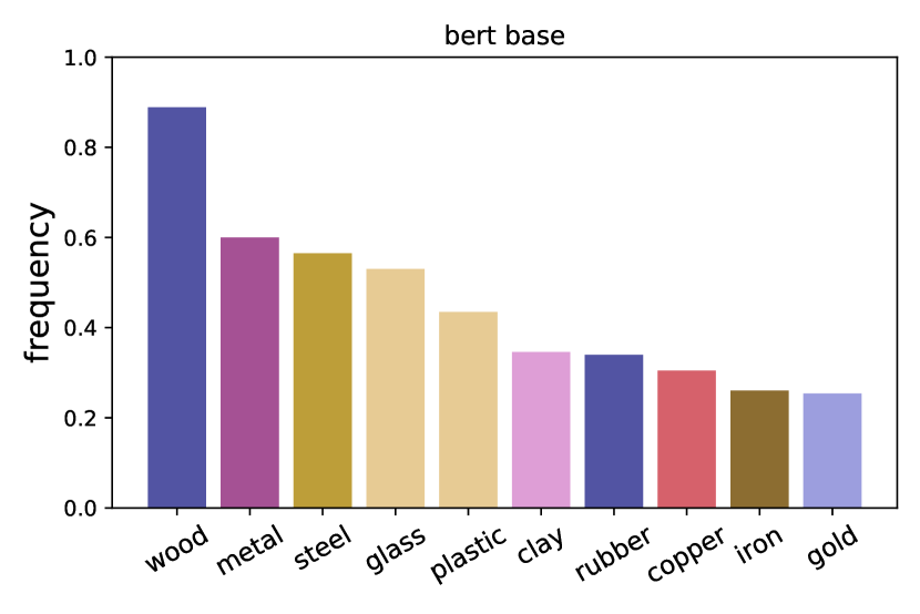
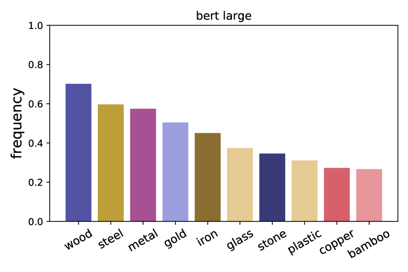
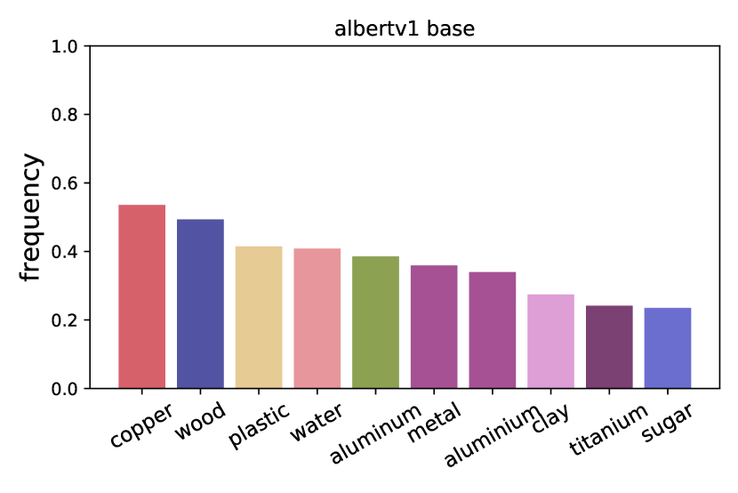
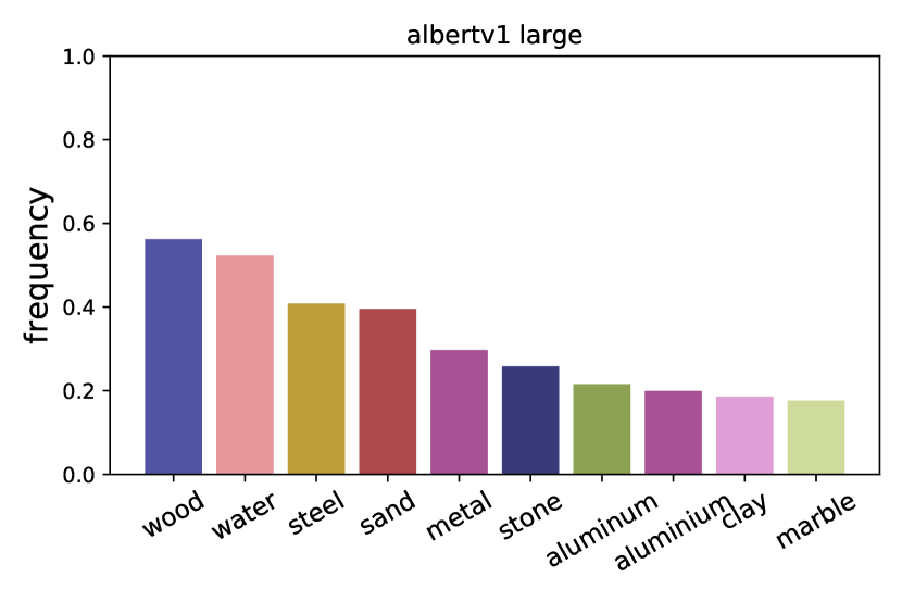
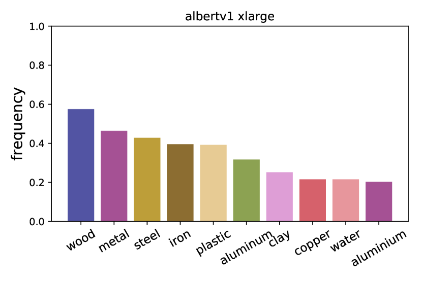
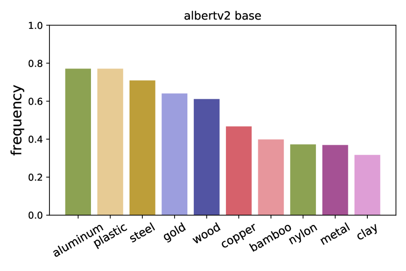
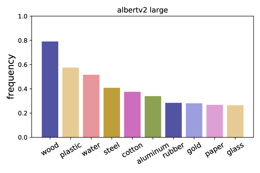
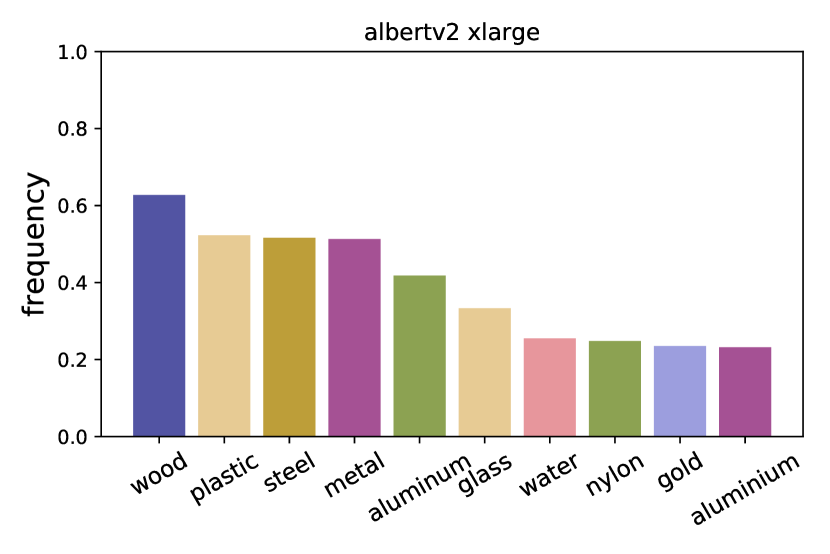
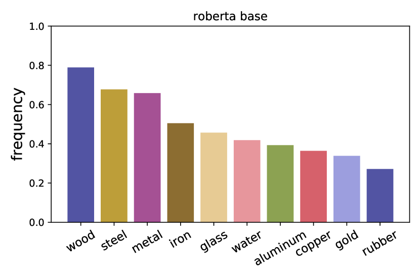
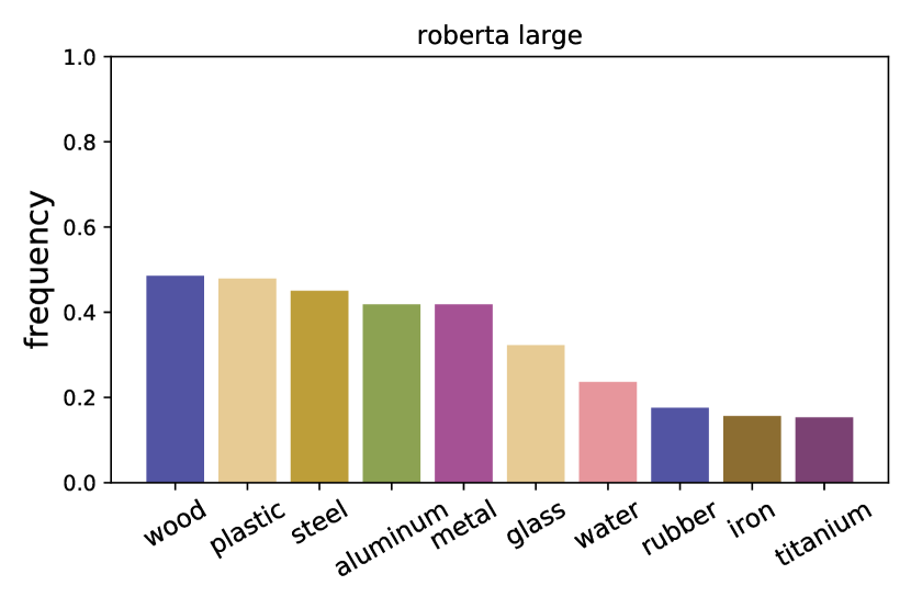
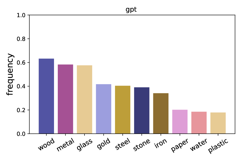
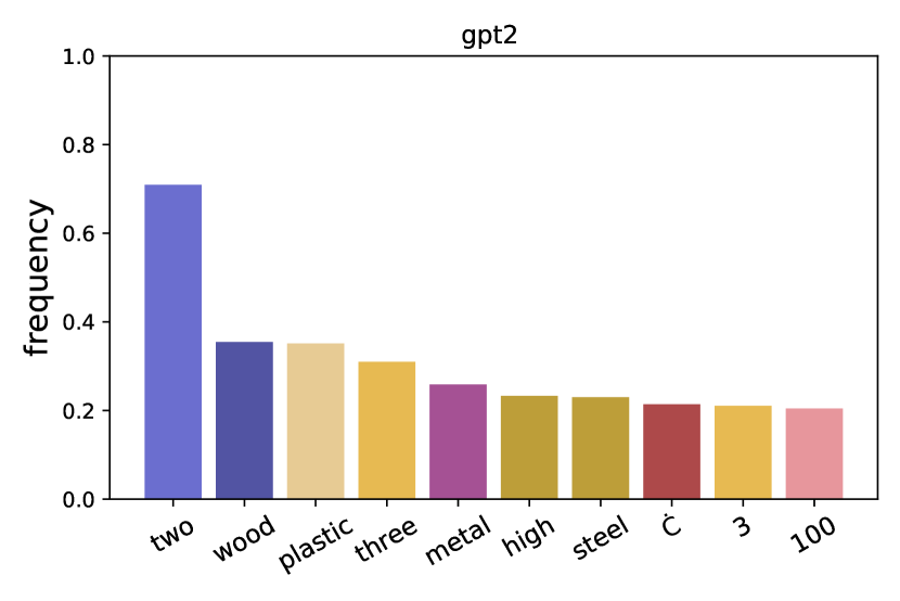
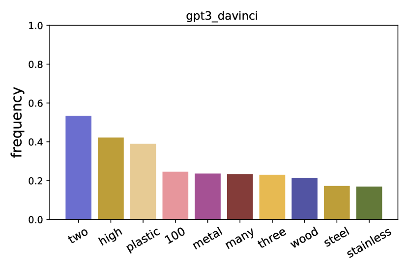
Appendix F Examples of Overlapping Synonym and Antonym

(a) ‘Hot’

(b) ‘Good’

(c) ‘Blue’

(d) ‘Weak’

(e) ‘Friend’

(f) ‘Short’

(g) ‘Spring’

(h) ‘Strength’

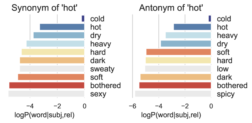
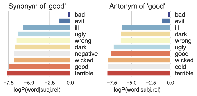
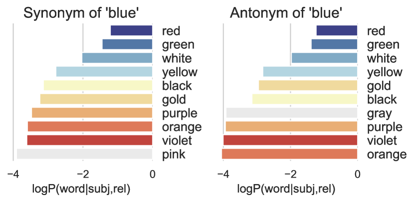
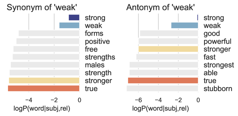
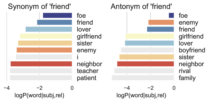
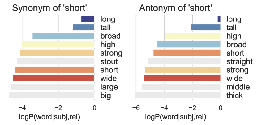
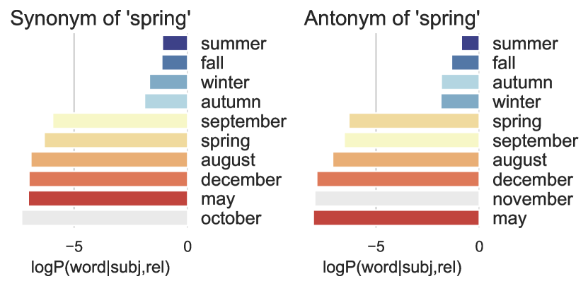
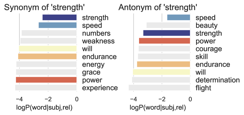
Appendix G Impact of the Finetuning on ConceptNet

Table 7: Results of the fine-tuned BERT_base $hits@K$ metric on the folds for each relation in ConceptNet.

Relations	$hits@K$
	Fold 0			Fold 1			Fold 1
	1	10	100	1	10	100	1	10	100
RelatedTo	18.30	34.70	54.20	18.50	34.90	54.70	18.60	35.00	54.50
HasContext	37.60	74.30	95.40	37.50	74.40	95.40	38.20	74.50	95.50
IsA	39.60	65.40	83.60	39.10	64.70	83.20	39.70	64.80	83.20
DerivedFrom	57.00	80.70	88.70	58.40	81.60	89.10	57.80	81.00	88.60
Synonym	23.60	48.00	68.60	23.90	49.00	68.80	23.00	47.70	68.00
FormOf	77.20	88.70	92.00	76.70	88.60	91.80	75.90	88.10	91.90
EtymologicallyRelatedTo	20.90	35.40	48.90	19.70	33.00	44.90	19.10	32.80	45.60
SimilarTo	8.20	33.40	60.90	7.60	33.20	61.90	7.40	32.70	62.80
AtLocation	18.20	50.20	85.10	15.70	48.50	84.40	17.00	48.60	83.90
MannerOf	12.20	38.00	69.20	12.90	36.80	67.10	13.10	36.40	67.00
PartOf	10.70	32.70	62.20	9.30	33.70	64.40	9.90	35.20	63.80
Antonym	8.70	44.10	71.50	8.10	43.70	69.90	8.90	38.90	67.10
HasProperty	11.80	40.00	72.20	10.70	38.80	72.70	9.20	37.30	73.80
UsedFor	8.70	32.70	65.00	6.20	29.80	60.80	9.40	31.20	62.30
DistinctFrom	7.40	48.10	76.80	6.80	54.30	76.00	7.20	54.20	79.50
HasPrerequisite	4.90	21.60	54.60	3.90	18.80	51.50	2.30	14.40	46.70
HasSubevent	6.20	25.30	52.00	5.50	23.00	54.20	6.60	26.90	55.20
Causes	9.30	29.90	61.90	7.70	25.00	56.30	10.00	31.40	60.30
HasA	11.50	40.60	72.40	10.20	40.70	70.90	8.00	44.40	73.40
InstanceOf	22.40	38.80	61.20	19.10	36.40	57.90	19.90	38.90	58.80
CapableOf	15.10	43.90	68.30	15.60	42.40	69.80	15.40	42.80	68.80
MotivatedByGoal	3.40	18.60	41.20	6.20	21.90	43.30	3.80	17.70	51.60
MadeOf	26.50	60.20	84.70	19.20	60.60	83.80	17.80	52.50	73.30
Entails	9.50	28.60	58.30	4.70	25.60	54.70	3.60	21.70	54.20
Desires	12.70	30.20	49.20	3.10	15.60	35.90	8.20	27.90	42.60
NotHasProperty	6.50	26.10	54.30	9.80	25.50	47.10	8.00	32.00	58.00
CreatedBy	0.00	37.10	68.60	0.00	36.80	71.10	9.10	39.40	69.70
DefinedAs	12.50	45.80	70.80	5.60	44.40	61.10	4.80	19.00	57.10
NotDesires	0.00	9.10	27.30	14.30	23.80	28.60	0.00	27.30	31.80
NotCapableOf	33.30	58.30	83.30	23.10	53.80	76.90	16.70	50.00	66.70
LocatedNear	0.00	50.00	87.50	9.10	45.50	45.50	9.10	45.50	63.60
EtymologicallyDerivedFrom	33.30	50.00	50.00	16.70	16.70	16.70	22.20	22.20	22.20

Table 8: Results of the fine-tuned BERT_large $hits@K$ metric on the folds for each relation in ConceptNet.

Relations	$hits@K$
	Fold 0			Fold 1			Fold 2
	1	10	100	1	10	100	1	10	100
RelatedTo	20.70	38.70	59.00	20.80	39.00	59.30	21.00	39.20	59.00
HasContext	40.80	76.00	95.70	40.80	76.40	95.90	41.10	76.50	95.90
IsA	42.60	69.00	86.10	42.00	68.20	85.30	42.30	68.60	85.60
DerivedFrom	60.80	84.70	91.30	61.60	84.60	91.30	62.30	85.00	91.60
Synonym	24.80	53.30	73.30	25.20	53.40	73.20	24.30	52.60	72.90
FormOf	80.90	90.40	93.40	80.40	90.20	93.60	80.10	90.20	93.50
EtymologicallyRelatedTo	21.70	38.80	52.90	20.20	35.80	50.00	19.70	35.10	50.10
SimilarTo	10.90	37.90	66.00	10.50	37.00	65.50	10.00	38.40	67.10
AtLocation	21.50	58.60	87.80	20.10	57.20	88.00	20.80	55.50	86.30
MannerOf	14.90	43.70	73.10	14.80	42.20	72.50	13.20	42.10	71.80
PartOf	9.70	37.40	67.00	10.20	38.10	66.80	10.50	40.40	68.70
Antonym	25.60	59.60	80.50	22.60	56.00	80.60	23.10	53.60	76.70
HasProperty	14.40	46.20	76.70	15.00	42.60	76.30	13.20	40.80	77.80
UsedFor	11.80	36.40	67.80	8.20	31.90	63.20	10.20	35.30	65.60
DistinctFrom	18.30	57.30	82.50	16.90	59.90	80.40	19.30	61.10	81.30
HasPrerequisite	6.90	26.70	59.20	6.00	23.50	56.50	1.70	19.60	55.60
HasSubevent	8.00	25.00	57.40	6.70	25.80	60.60	9.50	28.30	63.30
Causes	10.30	38.40	68.30	13.70	33.10	64.80	12.40	37.20	65.20
HasA	12.20	38.80	74.10	9.10	43.50	73.30	8.70	46.50	74.10
InstanceOf	22.00	41.10	66.40	19.60	41.60	60.30	21.80	42.20	62.60
CapableOf	19.50	46.80	66.30	18.50	43.40	73.70	19.70	45.20	71.60
MotivatedByGoal	3.40	17.50	52.50	5.10	21.30	57.90	3.20	24.70	59.70
MadeOf	28.60	62.20	87.80	25.30	66.70	88.90	20.80	51.50	78.20
Entails	8.30	26.20	59.50	3.50	23.30	62.80	4.80	25.30	60.20
Desires	20.60	33.30	65.10	3.10	20.30	39.10	13.10	24.60	49.20
NotHasProperty	19.60	37.00	80.40	13.70	31.40	54.90	12.00	40.00	70.00
CreatedBy	5.70	42.90	68.60	2.60	36.80	73.70	12.10	39.40	78.80
DefinedAs	25.00	50.00	79.20	5.60	50.00	83.30	4.80	47.60	90.50
NotDesires	0.00	4.50	31.80	14.30	23.80	33.30	13.60	27.30	45.50
NotCapableOf	25.00	58.30	91.70	30.80	46.20	76.90	25.00	33.30	75.00
LocatedNear	0.00	75.00	100.00	9.10	36.40	63.60	9.10	36.40	81.80
EtymologicallyDerivedFrom	50.00	50.00	50.00	16.70	16.70	16.70	22.20	22.20	22.20

Table 9: Comparison of macro average hits@K on pretrained and fune-tuned BERT models. Herin, Avg. indicates average.

Train Status	Model	Avg. Type	Hits@K
			1				10				100
			Fold 0	Fold 1	Fold 2	Avg.*	Fold 0	Fold 1	Fold 2	Avg.	Fold 0	Fold 1	Fold 2	Avg.
Pretrained	BERTbase	Micro	6.67	5.05	6.19	5.97	17.72	16.31	17.38	17.14	36.13	33.78	34.80	34.90
		Macro	7.93	7.74	7.79	7.82	19.69	19.65	19.62	19.65	37.29	37.25	37.21	37.25
	BERTlarge	Micro	8.00	5.51	7.31	6.94	20.03	17.65	18.27	18.65	38.17	36.31	36.07	36.85
		Macro	7.27	7.16	7.24	7.22	19.31	19.27	19.19	19.26	37.09	36.90	36.88	36.96
Fine-tuned	BERTbase	Micro	17.73	16.40	16.25	16.79	42.52	40.67	40.39	41.19	66.87	62.82	63.80	64.50
		Macro	29.58	29.60	29.77	29.65	52.20	52.22	52.16	52.19	70.88	70.97	70.89	70.91
	BERTlarge	Micro	21.39	19.14	19.55	20.03	46.93	43.63	43.93	44.83	72.23	68.20	70.23	70.22
		Macro	32.41	32.35	32.53	32.43	55.86	55.79	55.96	55.87	74.28	74.26	74.23	74.26

• Average of the performances of Fold 1, 2 and 3

Table 10: Results of missed prediction ratio at top K predictions of fine-tuned BERT models between the opposite relations.

		Miss@K*
		1			10			100
Model		Fold 0	Fold 1	Fold 2	Fold 0	Fold 1	Fold 2	Fold 0	Fold 1	Fold 2
	BERTbase	3.33	2.89	3.87	29.57	28.48	31.22	57.35	57.50	54.98
Synonym / Antonym	BERTlarge	4.42	4.21	4.36	29.53	29.63	30.35	56.34	58.43	58.21
	BERTbase	17.16	13.63	13.63	37.56	35.20	35.24	58.91	56.75	57.78
Antonym / Synonym	BERTlarge	8.69	8.57	8.20	31.50	27.40	28.24	55.26	49.87	52.70

• Miss@K = The ratio of words that are considered right when graded with the opposite relation (undesirable) in top K predictions.

Appendix H Comparative Studies with respect to the Lexical Similarities of a Question and a Context

(i) 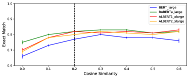(j)

Figure 4: Results on the word overlapping rate and the performance of RC models: (a) shows results of the has answer questions of SQuAD 2.0 and (b) shows results of ReCoRD.

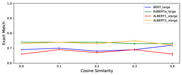
This section analyzes the correlation between the lexical overlap of a question and a context, and performances on the question. First, we measure the degree of the lexical variation based on the similarity between a question and a context. Specifically, a low similarity between a question and a context indicates a high lexical variation, and vice versa. For this, we use cosine similarity between term frequency-inverse document frequency (TF-IDF) term-weighted uni-gram bag-of-words vectors [59]. Then, we measure the difficulty level of a question based on the performance of the MNLM-based RC models.

Table 11: Examples of easy questions and hard questions on the has answer questions of SQuAD.

Similarity*	Question	Answer	Context
$>0.6$	In what year did Savery patent his steam pump?	1698	… In 1698 Thomas Savery patented a steam pump that used steam in direct contact with the water being pumped. …
$<0.1$	Which country was the last to receive the disease?	northwestern Russia	From Italy, the disease spread northwest across Europe, … Finally it spread to northwestern Russia in 1351. …

• Cosine similarity between TF-IDF term weighted uni-gram vectors of the question and the context

Appendix I Details on the Reading Comprehension Question Types

Table 12: Examples and descriptions for the question type of the has answer questions. The main clues for the categorization of the questions are colored.

Question Types	Description	Example
Synonymy	There is a clear correspondence between question and context.	Question: Which entity is the secondary legislative body? Context: … The second main legislative body is the Council, which is composed of different ministers of the member states. …
Commonsense knowledge	Commonsense knowledge is required to solve the question.	Question: Where is the Asian influence strongest in Victoria? Context: … Many Chinese miners worked in Victoria, and their legacy is particularly strong in Bendigo and its environs. …
No semantic variation	There is no semantic variation such as synonymy or commonsense knowledge.	Question: Who are the un-elected subordinates of member state governments? Context: … This means Commissioners are, through the appointment process, the unelected subordinates of member state governments. …
Multi-sentence reasoning	Hints for solving questions are shattered in multiple sentences.	Question: Why did France choose to give up continental lands? Context: … France chose to cede the former, … They viewed the economic value of the Caribbean islands’ sugar cane …
Typo	There exist typing errors in the question or context.	Question: What kind of measurements define accelerlations? Context… Accelerations can be defined through kinematic measurements. …
Others	The labeled answer is incorrect.	Question: Who won the battle of Lake George? Context: … The battle ended inconclusively, with both sides withdrawing from the field. …

Appendix J Supplementary Results on Section 5.1

(a) BERT_base

(b) BERT_large

(c) ALBERT1_base

(d) ALBERT1_large

(e) ALBERT1_xlarge

Figure 5: The proportion of predicted objects are in top 100 predictions for each model: (a) BERT_base, (b) BERT_large, (c) ALBERT1_base, (d) ALBERT1_large, (e) ALBERT1_xlarge. X-axis indicates frequency with which subject and object entities are observed together. Y-axis is the proportion of which the answer object can be found in top 100 model’s prediction for each frequency section. Blue bars indicate that the answer is in the top 100 predictions, while orange bars mean that the answer is not in the top 100 predictions. The results show that joint frequency of subject and object apparently affects the knowledge probing performance.

(a) BERT_base

(b) BERT_large

(c) ALBERT1_base

(d) ALBERT1_large

(e) ALBERT1_xlarge

Figure 6: Correlations of the joint frequency of subject and object, and frequency of subject: (a) BERT_base, (b) BERT_large, (c) ALBERT1_base, (d) ALBERT1_large, (e) ALBERT1_xlarge. X-axis indicates frequency with which subject and object entities are observed together. Y-axis intends the frequency of the subject. Values of heatmap means the proportion of which the answer object can be found in top 100 model’s prediction for each frequency grid. The results show that the performance increases as the subject observation frequency is lower in the same joint frequency section of subject and object.

(a) BERT_base

(b) BERT_large

(c) ALBERT1_base

(d) ALBERT1_large

(e) ALBERT1_xlarge

Figure 7: Correlations of the joint frequency of subject and object, and frequency of subject: (a) BERT_base, (b) BERT_large, (c) ALBERT1_base, (d) ALBERT1_large, (e) ALBERT1_xlarge. X-axis indicates frequency with which subject and object entities are observed together. Y-axis intends the frequency of the subject. Values of heatmap means the proportion of which the answer object can be found in top k model’s prediction for each frequency grid. Herein, the ‘k’ indicates the number of objects of a given subject and relation pair. The results show that the performance increases as the subject observation frequency is lower in the same joint frequency section of subject and object.

Appendix K Details on the Integrating External Commonsense Repository

1:An input question (Q), An input context (C), target knowledge (K) and templates (T)

2:$Q^{*}\leftarrow Q$; $C^{*}\leftarrow C$

3:for $K_{i}$ in $K$ do

4:     $Subject,Relation,Object\leftarrow K_{i}$

5:     if $(Q^{*},C^{*})$ in ReCoRD then

6:         $T_{Relation}\leftarrow T[Relation]$

7:         $T^{*}_{Relation}\leftarrow Replace(T_{Relation},``[[SUBJ]]",Subject)$

8:         $T^{*}_{Relation}\leftarrow Replace(T^{*}_{Relation},``[[OBJ]]",Object)$

9:         $C^{*}\leftarrow C^{*}+``@highlight^{\prime\prime}+T^{*}_{Relation}$

10:     else if $Subject$ in $Q$ and $Object$ in $C$ then

11:         $Q^{*}\leftarrow IntegrateKnowledgeIntoText(Q^{*},K_{i},T)$

12:     else if $Subject$ in $C$ and $Object$ in $Q$ then

13:         $C^{*}\leftarrow IntegrateKnowledgeIntoText(C^{*},K_{i},T)$

14:     end if

15:end for

16:Return $(Q^{*},C^{*})$

Algorithm 1 Pseudo code for the knowledge integration procedure

1:An input text (I), An input knowledge triple (k), and templates (T)

2:$Subject,Relation,Object\leftarrow k$

3:$i\leftarrow FindFirstIndex(Subject,I)$

4:$T_{Relation}\leftarrow T[Relation]$

5:$T^{*}_{Relation}\leftarrow Replace(T_{Relation},$“[[SUBJ]]",“which"$)$

6:$T^{*}_{Relation}\leftarrow Replace(T_{Relation},$ “[[OBJ]]"$,Object)$

7:$I^{*}\leftarrow I[:i]+T^{*}_{Relation}+I[i+1:]$

8:Return $I^{*}$

Algorithm 2 Pseudo code for the IntegrateKnowledgeIntoText function

References

- [1] Winograd, T. Understanding natural language. Cognitive psychology 3, 1–191 (1972).
- [2] Richardson, M., Burges, C. J. & Renshaw, E. Mctest: A challenge dataset for the open-domain machine comprehension of text. In Proceedings of the Conference on Empirical Methods in Natural Language Processing, 193–203 (2013).
- [3] Radford, A., Narasimhan, K., Salimans, T. & Sutskever, I. Improving language understanding by generative pre-training. Technical Report, OpenAi (2018).
- [4] Devlin, J., Chang, M.-W., Lee, K. & Toutanova, K. Bert: Pre-training of deep bidirectional transformers for language understanding. In Proceedings of the Conference of the North American Chapter of the Association for Computational Linguistics: Human Language Technologies, 4171–4186 (2019).
- [5] Shi, X., Padhi, I. & Knight, K. Does string-based neural mt learn source syntax? In Proceedings of the Conference on Empirical Methods in Natural Language Processing, 1526–1534 (2016).
- [6] Adi, Y., Kermany, E., Belinkov, Y., Lavi, O. & Goldberg, Y. Fine-grained analysis of sentence embeddings using auxiliary prediction tasks. In Proceedings of the International Conference on Learning Representations (2017).
- [7] Perone, C. S., Silveira, R. & Paula, T. S. Evaluation of sentence embeddings in downstream and linguistic probing tasks. arXiv preprint arXiv:1806.06259 (2018).
- [8] Conneau, A., Kruszewski, G., Lample, G., Barrault, L. & Baroni, M. What you can cram into a single &!#* vector: Probing sentence embeddings for linguistic properties. In Proceedings of Annual Meeting of the Association for Computational Linguistics, vol. 1, 2126–2136 (2018).
- [9] Sahin, G. G., Vania, C., Kuznetsov, I. & Gurevych, I. Linspector: Multilingual probing tasks for word representations. Computational Linguistics 46, 335–385 (2019).
- [10] Hewitt, J. & Manning, C. D. A structural probe for finding syntax in word representations. In Proceedings of the Conference of the North American Chapter of the Association for Computational Linguistics: Human Language Technologies, 4129–4138 (2019).
- [11] Liu, N. F., Gardner, M., Belinkov, Y., Peters, M. E. & Smith, N. A. Linguistic knowledge and transferability of contextual representations. In Proceedings of the Conference of the North American Chapter of the Association for Computational Linguistics: Human Language Technologies, 1073–1094 (2019).
- [12] Hahn, M. & Baroni, M. Tabula nearly rasa: Probing the linguistic knowledge of character-level neural language models trained on unsegmented text. Transactions of the Association for Computational Linguistics 7, 467–484 (2019).
- [13] Tenney, I. et al. What do you learn from context? probing for sentence structure in contextualized word representations. In Proceedings of the International Conference on Learning Representations (2019).
- [14] Tenney, I., Das, D. & Pavlick, E. Bert rediscovers the classical nlp pipeline. In Proceedings of the Annual Meeting of the Association for Computational Linguistics, 4593–4601 (2019).
- [15] Manning, C. D., Clark, K., Hewitt, J., Khandelwal, U. & Levy, O. Emergent linguistic structure in artificial neural networks trained by self-supervision. Proceedings of the National Academy of Sciences (2020).
- [16] Kim, T., Choi, J., Edmiston, D. & Lee, S.-g. Are pre-trained language models aware of phrases? simple but strong baselines for grammar induction. In Proceedings of the International Conference on Learning Representations (2020).
- [17] Nilsson, N. J. & Nilsson, N. J. Artificial intelligence: a new synthesis (Morgan Kaufmann, 1998).
- [18] Mihaylov, T. & Frank, A. Knowledgeable reader: Enhancing cloze-style reading comprehension with external commonsense knowledge. In Proceedings of the Annual Meeting of the Association for Computational Linguistics, 821–832 (2018).
- [19] Davison, J., Feldman, J. & Rush, A. M. Commonsense knowledge mining from pretrained models. In Proceedings of the Conference on Empirical Methods in Natural Language Processing and International the Joint Conference on Natural Language Processing, 1173–1178 (2019).
- [20] Speer, R., Chin, J. & Havasi, C. Conceptnet 5.5: an open multilingual graph of general knowledge. In Proceedings of the AAAI Conference on Artificial Intelligence, 4444–4451 (2017).
- [21] Liu, Y. et al. Roberta: A robustly optimized bert pretraining approach. arXiv preprint arXiv:1907.11692 (2019).
- [22] Lan, Z. et al. Albert: A lite bert for self-supervised learning of language representations. In Proceedings of the International Conference on Learning Representations (2019).
- [23] Vaswani, A. et al. Attention is all you need. In Proceedings of the Advances in Neural Information Processing Systems, 5998–6008 (2017).
- [24] Schuster, M. & Nakajima, K. Japanese and korean voice search. In Proceeding of the IEEE International Conference on Acoustics, Speech and Signal Processing, 5149–5152 (2012).
- [25] Zhu, Y. et al. Aligning books and movies: Towards story-like visual explanations by watching movies and reading books. In Proceedings of the IEEE International Conference on Computer Vision, 19–27 (2015).
- [26] Sennrich, R., Haddow, B. & Birch, A. Neural machine translation of rare words with subword units. In Proceedings of the Annual Meeting of the Association for Computational Linguistics, 1715–1725 (2016).
- [27] Nagel, S. Cc-news. http://web.archive.org/save/http://commoncrawl.org/2016/10/newsdataset-available (2016).
- [28] Gokaslan, A. & Cohen, V. Openwebtext corpus. http://web.archive.org/save/https://skylion007.github.io/OpenWebTextCorpus/ (2016).
- [29] Trinh, T. H. & Le, Q. V. A simple method for commonsense reasoning. arXiv preprint arXiv:1806.02847 (2018).
- [30] Radford, A. et al. Language models are unsupervised multitask learners. Technical Report, OpenAi (2019).
- [31] Brown, T. B. et al. Language models are few-shot learners. Technical Report, OpenAi (2020).
- [32] Da, J., Bras, R. L., Lu, X., Choi, Y. & Bosselut, A. Understanding few-shot commonsense knowledge models. arXiv preprint arXiv:2101.00297 (2021).
- [33] Sainz, O. & Rigau, G. Ask2transformers: Zero-shot domain labelling with pretrained language models. In Proceedings of the 11th Global Wordnet Conference, 44–52 (2021).
- [34] OpenAI. Openai gpt3 api link. https://beta.openai.com/ (2020).
- [35] Singh, P. et al. Open mind common sense: Knowledge acquisition from the general public. In Proceedings of the International Conference on Ontologies, Databases, and Applications of Semantics for Large Scale Information Systems, 1223–1237 (2002).
- [36] Wang, L., Sun, M., Zhao, W., Shen, K. & Liu, J. Yuanfudao at semeval-2018 task 11: Three-way attention and relational knowledge for commonsense machine comprehension. In Proceedings of the International Workshop on Semantic Evaluation, 758–762 (2018).
- [37] Guan, J., Wang, Y. & Huang, M. Story ending generation with incremental encoding and commonsense knowledge. In Proceedings of the AAAI Conference on Artificial Intelligence, vol. 33, 6473–6480 (2019).
- [38] Talmor, A., Herzig, J., Lourie, N. & Berant, J. Commonsenseqa: A question answering challenge targeting commonsense knowledge. In Proceedings of the Conference of the North American Chapter of the Association for Computational Linguistics: Human Language Technologies, 4149–4158 (2019).
- [39] Petroni, F. et al. Language models as knowledge bases? In Proceedings of the Conference on Empirical Methods in Natural Language Processing and the International Joint Conference on Natural Language Processing, 2463–2473 (2019).
- [40] Kassner, N. & Schütze, H. Negated and misprimed probes for pretrained language models: Birds can talk, but cannot fly. In Proceedings of the Annual Meeting of the Association for Computational Linguistics, 7811–7818 (2020).
- [41] Jiang, Z., Xu, F. F., Araki, J. & Neubig, G. How can we know what language models know? Transactions of the Association for Computational Linguistics 8, 423–438 (2020).
- [42] Shin, T., Razeghi, Y., Logan IV, R. L., Wallace, E. & Singh, S. Eliciting knowledge from language models using automatically generated prompts. In Proceedings of the 2020 Conference on Empirical Methods in Natural Language Processing, 4222–4235 (2020).
- [43] Bouraoui, Z., Camacho-Collados, J. & Schockaert, S. Inducing relational knowledge from bert. In Proceedings of the AAAI Conference on Artificial Intelligence, 7456–7463 (2020).
- [44] Speer, R. Conceptnet 5.6.0. https://s3.amazonaws.com/conceptnet/downloads/2018/edges/conceptnet-assertions-5.6.0.csv.gz (2018).
- [45] Chapelle, C. A. & Abraham, R. G. Cloze method: What difference does it make? Language Testing 7, 121–146 (1990).
- [46] Zhong, Z., Friedman, D. & Chen, D. Factual probing is [mask]: Learning vs. learning to recall. In Proceedings of the North American Association for Computational Linguistics (2021).
- [47] Wallace, E., Feng, S., Kandpal, N., Gardner, M. & Singh, S. Universal adversarial triggers for attacking and analyzing NLP. In Proceedings of the Empirical Methods in Natural Language Processing (2019).
- [48] Speer, R. Open mind common sense data. https://s3.amazonaws.com/conceptnet/downloads/2018/omcs-sentences-more.txt (2018).
- [49] Bordes, A., Usunier, N., Garcia-Duran, A., Weston, J. & Yakhnenko, O. Translating embeddings for modeling multi-relational data. In Proceedings of the Advances in Neural Information Processing Systems, 2787–2795 (2013).
- [50] Rajpurkar, P., Jia, R. & Liang, P. Know what you don’t know: Unanswerable questions for squad. In Proceedings of the Annual Meeting of the Association for Computational Linguistics, 784–789 (2018).
- [51] Zhang, S. et al. Record: Bridging the gap between human and machine commonsense reading comprehension. arXiv preprint arXiv:1810.12885 (2018).
- [52] Wang, A. et al. Superglue: a stickier benchmark for general-purpose language understanding systems. In Proceedings of the International Conference on Neural Information Processing Systems, 3266–3280 (2019).
- [53] van Aken, B., Winter, B., Löser, A. & Gers, F. A. How does bert answer questions? a layer-wise analysis of transformer representations. In Proceedings of the 28th ACM International Conference on Information and Knowledge Management, 1823–1832 (2019).
- [54] Clark, K., Luong, M.-T., Le, Q. V. & Manning, C. D. Electra: Pre-training text encoders as discriminators rather than generators. In Proceedings of the International Conference on Learning Representations (2020).
- [55] Rajpurkar, P., Zhang, J., Lopyrev, K. & Liang, P. Squad: 100,000+ questions for machine comprehension of text. In Proceedings of the Conference on Empirical Methods in Natural Language Processing, 2383–2392 (2016).
- [56] Mintz, M., Bills, S., Snow, R. & Jurafsky, D. Distant supervision for relation extraction without labeled data. In Proceedings of the Joint Conference of the Annual Meeting and the International Joint Conference on Natural Language Processing, 1003–1011 (2009).
- [57] Pennington, J., Socher, R. & Manning, C. GloVe: Global vectors for word representation. In Proceedings of the Conference on Empirical Methods in Natural Language Processing, 1532–1543 (2014).
- [58] Powers, D. M. Applications and explanations of zipf’s law. In Proceedings of the New methods in language processing and computational natural language learning (1998).
- [59] Manning, C., Raghavan, P. & Schütze, H. Introduction to information retrieval. Natural Language Engineering 16, 100–103 (2010).