Non-perturbative treatment of open-system multi-time expectation values
in Gaussian bosonic environments

Abstract

We determine the conditions for the equivalence between the multi-time expectation values of a general finite-dimensional open quantum system when interacting with, respectively, an environment undergoing a free unitary evolution or a discrete environment under a free evolution fixed by a proper Gorini-Kossakowski-Lindblad-Sudarshan generator. We prove that the equivalence holds if both environments are bosonic and Gaussian and if the one- and two-time correlation functions of the corresponding interaction operators are the same at all times. This result leads to a non-perturbative evaluation of the multi-time expectation values of operators and maps of open quantum systems interacting with a continuous set of bosonic modes by means of a limited number of damped modes, thus setting the ground for the investigation of open-system multi-time quantities in fully general regimes.

I Introduction

The complete statistical description of an open quantum system calls for the characterization of multi-time expectation values [1, 2]. As significant examples, mean values of operators at different times, i.e., multi-time correlation functions, yield optical spectra that are of central interest in many physical applications [3], while multi-time expectation values of completely positive trace non-increasing maps define the joint probability distributions associated with sequential measurements at different times [4].

The quantum regression theorem [5, 6, 7] fixes the dynamical equations for multi-time expectation values from those of single-time expectation values, that is, of the quantum state itself. On the other hand, the validity of the quantum regression theorem can be proven only under quite restrictive conditions [8], which essentially imply that the system-environment correlations created by the interaction do not impact the multi-time statistics [9], or for rather specific forms of the system-environment coupling [10, 11, 12]. Treatments of multi-time expectation values of open quantum systems beyond the quantum regression theorem mainly include the use of perturbative techniques [13, 14, 15, 16, 17, 18, 19] or the analysis of specific models [10, 20, 21, 11, 12], but no general approach able to deal with generic dynamical regimes and physical systems is currently available.

Here, we establish a systematic non-perturbative method to evaluate open-system multi-time expectation values by proving the equivalence between two different system-environment configurations, see Fig.1. In the first one, the system and the (in general, continuous) environment are evolved by a joint unitary dynamics, while in the second one the same system interacts with an environment consisting of a set of discrete modes and undergoing an evolution fixed by a Gorini-Kossakowski-Lindblad-Sudarshan (GKLS) generator [22, 23]. Explicitly, we prove that the multi-time expectation values of any sequence of open-system operators are identical in the two configurations, provided that the environments are bosonic and Gaussian, and that the one- and two-time correlation functions of the environmental interaction operators coincide under the corresponding free evolutions.

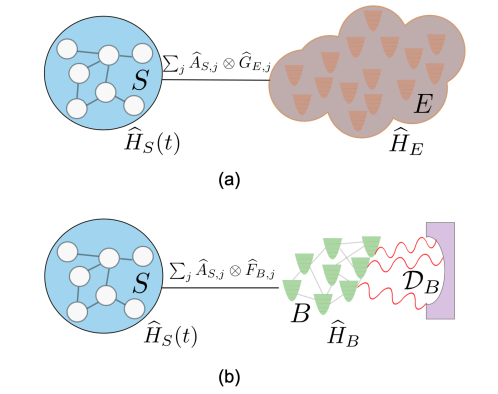
Figure 1: The two configurations we are considering. (a) A system $S$ interacts with a continuum (or countably infinite number) of bosonic modes $E$ undergoing a unitary free evolution. (b) The same system $S$ interacts with a finite number of modes $B$ whose free evolution is determined by a master equation of GKSL type.

As a result, under the conditions set out above, an open quantum system interacting with a continuous set of bosonic modes may be represented equivalently by a discrete set of auxiliary bosonic modes which undergo a GKLS dynamics. The specific features of the set of auxiliary damped modes, i.e., their frequencies and couplings, can be determined via the procedure developed in [24], which relies on a fit of the two-time correlation functions of the continuous bath with a finite number of exponentials, weighted by possibly complex coefficients. Starting from the equivalence theorem proved here, it is thus possible to evaluate in a non-perturbative way multi-time expectation values in generic parameter regimes. This extends the approach put forward in [25] and further developed in [24], which concerned the reduced dynamics of the unitary and GKLS configurations and thus ensured the identity between single-time expectation values only; an analogous approach for fermionic baths, addressing both single- and multi-time expectation values has been introduced in [26]. Very recently [27], building upon the equivalence theorem proved here, 2D electronic spectra for a dimeric complex have been evaluated for a realistic parameter regime.

II Unitary and GKLS environments and their multi-time expectation values

We start by introducing the two open-system configurations characterized by, respectively, a unitary and a non-unitary (GKLS) free-evolving environment, along with the definitions of the relevant quantities, which will be the object of the equivalence theorem presented in the next section.

Consider first any finite dimensional open quantum system $S$ with dimension $d_{S}$ interacting with the bosonic environment $E$ according to the global Hamiltonian

$$\widehat{H}_{SE}(t)=\widehat{H}_{S}(t)+\widehat{H}_{E}+\sum^{\kappa}_{j=1}\widehat{A}_{S,j}\otimes\widehat{G}_{E,j},$$ (1)

where $\kappa\leq d_{S}^{2}$, and we allow for a possible time dependence in the free system-Hamiltonian $\widehat{H}_{S}(t)$, so that general time dependent controls are included in our treatment; $\widehat{H}_{E}$ is instead the Hamiltonian of the bosonic environment on which we do not make, for the time being, any particular assumptions. Moreover, we assume an initial factorized state,

$$\varrho_{SE}(0)=\varrho_{S}(0)\otimes\varrho_{E}(0),$$ (2)

so that the dynamics on $S$ is completely positive [1]. Our main focus is the general (time-ordered) $n$-time expectation value

$$\langle O_{n}(t_{n})\ldots O_{1}(t_{1});O^{\prime}_{1}(t_{1})\ldots O^{\prime}_{n}(t_{n})\rangle_{U}=$$ (3)

$$\hskip 56.9055pt\operatorname{Tr}_{SE}\left\{\mathcal{U}^{\dagger}_{SE}(t_{n})\left[\widehat{O}_{n}\right]\ldots\mathcal{U}^{\dagger}_{SE}(t_{1})\left[\widehat{O}_{1}\right]\varrho_{SE}(0)\mathcal{U}^{\dagger}_{SE}(t_{1})\left[\widehat{O}^{\prime}_{1}\right]\ldots\mathcal{U}^{\dagger}_{SE}(t_{n})\left[\widehat{O}^{\prime}_{n}\right]\right\},$$

with $t_{n}\geq\ldots\geq t_{1}\geq 0$, where $\widehat{O}_{k}$ is a short-hand notation for $\widehat{O}_{k}\otimes\mathbbm{1}_{E}$, $\widehat{O}_{1},\ldots{,}\widehat{O}_{n}$ and $\widehat{O}^{\prime}_{1}{,}\ldots{,}\widehat{O}^{\prime}_{n}$ are generic open-system operators and $\mathcal{U}^{\dagger}_{SE}(t)$ defines the $S-E$ unitary evolution in the Heisenberg picture

$$\mathcal{U}^{\dagger}_{SE}(t)[\widehat{O}]=\widehat{U}^{\dagger}_{SE}(t)\widehat{O}\widehat{U}_{SE}(t),\qquad\widehat{U}_{SE}(t)=T_{\leftarrow}e^{-i\int_{0}^{t}ds\widehat{H}_{SE}(s)},$$ (4)

with $T_{\leftarrow}$ the chronological time-ordering operator. Note that Eq.(3) defines the most general multi-time expectation values appearing in the description of the evolution of open quantum systems [28, 8, 29]; for $\widehat{O}^{\prime}_{1}=\ldots=\widehat{O}^{\prime}_{n}=\mathbbm{1}_{S}$ and self-adjoint $\widehat{O}_{1}\ldots\widehat{O}_{n}$ we recover the multi-time correlation functions of the observables associated with the latter operators [1], while for $\widehat{O}^{\prime}_{1}=\widehat{O}^{\dagger}_{1}{,}\ldots{,}\widehat{O}^{\prime}_{n}=\widehat{O}^{\dagger}_{n}$ we obtain the multi-time probabilities associated with a generic sequence of measurements [4, 30]; finally, identity operators appearing alternatively among the left and the right operators lead us to the definition of signals in multi-dimensional spectroscopy [27]. Introducing the unitary propagators in the Schrödinger picture

$$\mathcal{U}_{SE}(t,t^{\prime})[\varrho_{SE}]=\widehat{U}_{SE}(t,t^{\prime})\varrho_{SE}\widehat{U}^{\dagger}_{SE}(t,t^{\prime}),\qquad\widehat{U}_{SE}(t,t^{\prime})=\widehat{U}_{SE}(t)\widehat{U}^{\dagger}_{SE}(t^{\prime})=T_{\leftarrow}e^{-i\int_{t^{\prime}}^{t}ds\widehat{H}_{SE}(s)},$$ (5)

the definition in Eq.(3) can be expressed equivalently as

$$\langle O_{n}(t_{n})\ldots O_{1}(t_{1});O^{\prime}_{1}(t_{1})\ldots O^{\prime}_{n}(t_{n})\rangle_{U}=$$ (6)

$$\hskip 56.9055pt\operatorname{Tr}_{SE}\left\{\widehat{O}_{n}\mathcal{U}_{SE}(t_{n},t_{n-1})\left[\ldots\mathcal{U}_{SE}(t_{2},t_{1})\left[\widehat{O}_{1}\mathcal{U}_{SE}(t_{1})\left[\varrho_{SE}(0)\right]\widehat{O}^{\prime}_{1}\right]\ldots\right]\widehat{O}^{\prime}_{n}\right\}.$$

In addition, we consider the single-time expectation values of the environmental interaction terms,

$$G^{U}_{E,j}(t)=\operatorname{Tr}_{E}\left\{e^{i\widehat{H}_{E}t}\widehat{G}_{E,j}e^{-i\widehat{H}_{E}t}\varrho_{E}(0)\right\},$$ (7)

as well as the two-time correlation functions

$$C^{U}_{jj^{\prime}}(t+s,s) =\operatorname{Tr}_{E}\left\{e^{i\widehat{H}_{E}(t+s)}\widehat{G}_{E,j}e^{-i\widehat{H}_{E}(t+s)}e^{i\widehat{H}_{E}s}\widehat{G}_{E,j^{\prime}}e^{-i\widehat{H}_{E}s}\varrho_{E}(0)\right\}.$$ (8)

Crucially, the definitions of $G^{U}_{E,j}(t)$ and $C^{U}_{jj^{\prime}}(t+s,s)$ correspond to the general definitions in Eq.(3) but with respect to the free evolution of the environment, as fixed by $\widehat{H}_{E}$; thus, their explicit evaluation does not involve the solution of the full dynamics.

The second configuration we take into account consists of the same quantum system $S$ interacting with a bosonic environment $B$, such that the global evolution is fixed by the GKLS generator

$$\mathcal{L}_{SB}(t)[\varrho_{SB}] = -i\left[\widehat{H}_{SB}(t),\varrho_{SB}\right]+\mathcal{D}_{B}[\varrho_{SB}]=$$ (9)

$$-i\left[\widehat{H}_{SB}(t),\varrho_{SB}\right]+\sum_{j=1}^{\ell}\gamma_{j}\left(\widehat{L}_{B,j}\varrho_{SB}\widehat{L}_{B,j}^{\dagger}-\frac{1}{2}\left\{\widehat{L}_{B,j}^{\dagger}\widehat{L}_{B,j},\varrho_{SB}\right\}\right),$$

where the Hamiltonian term can be decomposed as

$$\widehat{H}_{SB}(t)=\widehat{H}_{S}(t)+\widehat{H}_{B}+\sum^{\kappa}_{j=1}\widehat{A}_{S,j}\otimes\widehat{F}_{B,j},$$ (10)

with $\widehat{H}_{B}$ the (yet unspecified) free-environment Hamiltonian, and $\gamma_{j}\geq 0$, ensuring the complete positivity of the evolution on $S+B$ [22, 23, 1]; note that $\ell$ is related with the number of degrees of freedom of B, and hence with the complexity of the non-unitary configuration. We stress that the dissipative term acts on $B$ only. Moreover, the free Hamiltonian of the open system ${\hat{H}}_{S}(t)$, as well as the operators $\widehat{A}_{S,j}$ acting on the open system side in the interaction part of the Hamiltonian $\widehat{H}_{SB}(t)$, are the same as those in $\widehat{H}_{SE}(t)$ (compare Eq. 1 and Eq. 10): in this sense, the open system is the same in the two configurations. We further assume a factorized initial state

$$\varrho_{SB}(0)=\varrho_{S}(0)\otimes\varrho_{B}(0),$$ (11)

which guarantees the complete positivity of the evolution on $S$. The general $n$-time expectation values under the GKLS evolution are defined as

$$\langle O_{n}(t_{n})\ldots O_{1}(t_{1});O^{\prime}_{1}(t_{1})\ldots O^{\prime}_{n}(t_{n})\rangle_{L}=$$ (12)

$$\hskip 56.9055pt\operatorname{Tr}_{SB}\left\{\widehat{O}_{n}\Lambda_{SB}(t_{n},t_{n-1})\left[\ldots\Lambda_{SB}(t_{2},t_{1})\left[\widehat{O}_{1}\Lambda_{SB}(t_{1})\left[\varrho_{SB}(0)\right]\widehat{O}^{\prime}_{1}\right]\ldots\right]\widehat{O}^{\prime}_{n}\right\},$$

with the propagators

$$\Lambda_{SB}(t,t^{\prime})=T_{\leftarrow}e^{\int_{t^{\prime}}^{t}\mathcal{L}_{SB}(s)}$$ (13)

with $\Lambda_{SB}(t)=\Lambda_{SB}(t,0)$; $\widehat{O}_{k}$ is now a short-hand notation for $\widehat{O}_{k}\otimes\mathbbm{1}_{B}$. As before, we also consider the one- and two-time correlation functions of the environmental interaction operators with respect to the “free” evolution of the environment (i.e., without taking into account the presence of the system $S$), which is now fixed by the GKLS generator on $B$

$$\mathcal{L}_{B}[\varrho_{B}]=-i\left[\widehat{H}_{B},\varrho_{B}\right]+\mathcal{D}_{B}[\varrho_{B}],$$ (14)

so that we have

$$F^{L}_{B,j}(t)=\operatorname{Tr}_{B}\left\{\widehat{F}_{B,j}e^{\mathcal{L}_{B}t}\left[\varrho_{B}(0)\right]\right\},$$ (15)

as well as the two-time correlation functions

$$C_{jj^{\prime}}^{L}(t+s,s)=\operatorname{Tr}_{B}\left\{\widehat{F}_{B,j}e^{\mathcal{L}_{B}t}\left[\widehat{F}_{B,j^{\prime}}e^{\mathcal{L}_{B}s}\left[\varrho_{B}(0)\right]\right]\right\}.$$ (16)

As stated earlier, we will restrict our attention to the case where both the environments $E$ and $B$ are Gaussian. In particular, we assume that

1. both the initial environmental states $\varrho_{E}(0)$ and $\varrho_{B}(0)$ are Gaussian states,

2. the environmental free Hamiltonians $\widehat{H}_{E}$ and $\widehat{H}_{B}$ are at most quadratic in the corresponding creation and annihilation operators,

3. the environmental coupling operators $\widehat{G}_{E,j}$ and $\widehat{F}_{B,j}$, as well as the Lindblad operators $\widehat{L}_{B,j}$ are linear in the creation and annihilation operators.

Crucially, these assumptions imply that the $n$-time correlation functions of the environmental interaction operators under the free evolution of the environment (generalizing the definitions in, respectively, Eq.(8) and Eq.(16)) can be expressed in terms of the corresponding one- and two-time correlation functions; in other terms, the environmental interaction operators are Gaussian operators with respect to the free dynamics [31]. In fact, assumptions ii) and iii) guarantee that the environmental interaction operators evolved via the free environmental evolution at a generic time are linear in the creation and annihilation operators, so that, using also assumption i), one can apply the Wick’s theorem and then express any environmental $n$-time correlation function in terms of one- and two-time correlation functions [32].

III Equivalence theorem

We can now formulate the equivalence theorem, which equates the open-system multi-time expectation values of the unitary configuration and those of the GKLS configuration, provided that the one- and two-time environmental correlation functions coincide.

Theorem.

Consider the same open system $S$ in the two configurations characterized by, respectively, Eqs. (1)-(8) and Eqs. (9)-(16), and with the same initial state $\varrho_{S}(0)$. If the bosonic environments $E$ and $B$ satisfy the assumptions i)-iii) above, and if

$$F^{L}_{B,j}(t)=G^{U}_{E,j}(t)\,\,\qquad\forall j\,\mbox{and }t\geq 0$$ (17)

and

$$C^{L}_{jj^{\prime}}(t+s,s)=C^{U}_{jj^{\prime}}(t+s,s)\,\,\qquad\forall j,j^{\prime}\mbox{ and }\forall t,s\geq 0,$$ (18)

then

$$\langle O_{n}(t_{n})\ldots O_{1}(t_{1});O^{\prime}_{1}(t_{1})\ldots O^{\prime}_{n}(t_{n})\rangle_{L}=\langle O_{n}(t_{n})\ldots O_{1}(t_{1});O^{\prime}_{1}(t_{1})\ldots O^{\prime}_{n}(t_{n})\rangle_{U}$$

$$\,\,\qquad\forall O_{1},\ldots O_{n},;O^{\prime}_{1}\ldots O^{\prime}_{n}\,\mbox{ and }\,\forall t_{n}\geq\ldots\geq t_{1}\geq 0.$$ (19)

Proof. The proof essentially follows the same steps of the proof for the one-time expectation values derived in [25], generalizing it to the multi-time case by means of induction, analogously to what is done in [26] for the fermionic case.

The key point is the introduction of a third configuration, which represents the unitary dilation [7] of the non-unitary configuration. Hence, consider the tripartite system $S-B-\tilde{E}$ given by the $S-B$ system introduced above and a continuous distribution of bosonic modes labelled by $\tilde{E}$. The tripartite system evolves unitarily by means of the Hamiltonian [33]

$$\widehat{H}_{SB\tilde{E}}(t) =\widehat{H}_{SB}(t)+\widehat{H}_{\tilde{E}}+\widehat{V}_{B\tilde{E}},$$

$$\widehat{H}_{\tilde{E}} =\sum^{\ell}_{j=1}\int_{-\infty}^{\infty}d\omega\,\omega\,\widehat{b}^{{\dagger}}_{\tilde{E}}(\omega,j)\widehat{b}_{\tilde{E}}(\omega,j),$$ (20)

$$\widehat{V}_{B\tilde{E}} =\sum^{\ell}_{j=1}\sqrt{-\frac{\gamma_{j}}{2\pi}}\int_{-\infty}^{\infty}d\omega\widehat{L}_{B,j}\widehat{b}^{{\dagger}}_{\tilde{E}}(\omega,j)-\widehat{L}^{{\dagger}}_{B,j}\widehat{b}_{\tilde{E}}(\omega,j),$$

where $\widehat{b}_{\tilde{E}}(\omega,j)$ and $\widehat{b}^{{\dagger}}_{\tilde{E}}(\omega,j)$ are bosonic annihilation and creation operators of a Fock space $\mathcal{H}_{\tilde{E},j}$,

$$\left[\widehat{b}_{\tilde{E}}(\omega,j),\widehat{b}^{{\dagger}}_{\tilde{E}}(\omega^{\prime},j^{\prime})\right]=\delta_{jj^{\prime}}\delta(\omega-\omega^{\prime});$$ (21)

the initial state is

$$\varrho_{SB\tilde{E}}(0)=\varrho_{SB}(0)\otimes|\>0_{\tilde{E}}\>\rangle\langle\>0_{\tilde{E}}\>|,$$ (22)

with $\varrho_{SB}(0)$ as in Eq. 11 and $\ket{0_{\tilde{E}}}=\otimes_{j=1}^{\ell}\ket{0_{j}}$ the vacuum state of the global Fock space associated with $\tilde{E}$, $\mathcal{H}_{\tilde{E}}=\otimes_{j=1}^{\ell}\mathcal{H}_{\tilde{E},j}$. The $n$-time expectation values of such a unitary evolution can be defined as (compare with Eq.(6))

$$\langle O_{n}(t_{n})\ldots O_{1}(t_{1});O^{\prime}_{1}(t_{1})\ldots O^{\prime}_{n}(t_{n})\rangle_{X}=$$ (23)

$$\hskip 56.9055pt\operatorname{Tr}_{SB\tilde{E}}\left\{\widehat{O}_{n}\widetilde{\mathcal{U}}(t_{n},t_{n-1})\left[\ldots\widetilde{\mathcal{U}}(t_{2},t_{1})\left[\widehat{O}_{1}\widetilde{\mathcal{U}}(t_{1})\left[\varrho_{SB\tilde{E}}(0)\right]\widehat{O}^{\prime}_{1}\right]\ldots\right]\widehat{O}^{\prime}_{n}\right\},$$

where $\widehat{O}_{k}$ is now a short-hand notation for $\widehat{O}_{k}\otimes\mathbbm{1}_{B\tilde{E}}$, and the subscript $X$ indicates that the expectation is taken over the extended $SB\tilde{E}$ space. Here $\widetilde{\mathcal{U}}(t,t^{\prime})$ is the propagator of the unitary dynamics on $S-B-\tilde{E}$ which reads

$$\widetilde{\mathcal{U}}(t,t^{\prime})\left[\varrho_{SB\tilde{E}}\right]=\widehat{U}_{SB\tilde{E}}(t,t^{\prime})\varrho_{SB\tilde{E}}\widehat{U}^{\dagger}_{SB\tilde{E}}(t,t^{\prime}),\qquad\widehat{U}_{SB\tilde{E}}(t,t^{\prime})=T_{\leftarrow}e^{-i\int_{t^{\prime}}^{t}ds\widehat{H}_{SB\tilde{E}}(s)};$$ (24)

finally, the one- and two-time correlation functions of the environmental interaction operators (that are still the $\widehat{F}_{B,j}$, as the interaction with $S$ is still given by $\widehat{H}_{SB}(t)$) with respect to the free unitary dynamics on $B-\tilde{E}$ fixed by the Hamiltonian

$$\widehat{H}_{B\tilde{E}}=\widehat{H}_{B}+\widehat{H}_{\tilde{E}}+\widehat{V}_{B\tilde{E}}$$ (25)

are

$$F^{X}_{B,j}(t)=\operatorname{Tr}_{B\tilde{E}}\left\{e^{i\widehat{H}_{B\tilde{E}}t}\widehat{F}_{B,j}\otimes\mathbbm{1}_{\tilde{E}}e^{-i\widehat{H}_{B\tilde{E}}t}\varrho_{B\tilde{E}}(0)\right\}$$ (26)

and

$$C^{X}_{jj^{\prime}}(t+s,s) =\operatorname{Tr}_{B\tilde{E}}\left\{e^{i\widehat{H}_{B\tilde{E}}(t+s)}\widehat{F}_{B,j}\otimes\mathbbm{1}_{\tilde{E}}e^{-i\widehat{H}_{B\tilde{E}}(t+s)}e^{i\widehat{H}_{B\tilde{E}}s}\widehat{F}_{B,j^{\prime}}\otimes\mathbbm{1}_{\tilde{E}}e^{-i\widehat{H}_{B\tilde{E}}s}\varrho_{B\tilde{E}}(0)\right\}.$$

To prove the theorem, the first observation is that the multi-time expectation values of two unitary configurations with the same open system $S$ and initial state $\varrho_{S}(0)$ coincide if the corresponding $n$-time correlation functions of the environmental interaction operators under the respective free dynamics are the same; this can be shown, for example, via the Dyson expansion [25]. But then, since we are dealing with Gaussian environments [34] – so that the $n$-time correlation functions are uniquely determined by the one- and two-time correlation functions – we immediately have the following implication

$$\left.\begin{tabular}[]{ccc}$F^{X}_{B,j}(t)$&$=$&$G^{U}_{E,j}(t)$\\ $C^{X}_{jj^{\prime}}(t+s,s)$&$=$&$C^{U}_{jj^{\prime}}(t+s,s)$\end{tabular}\right\} \,\,\,\forall j,j^{\prime}\,\forall t,s\geq 0$$ (29)

$$\Longrightarrow\quad\langle O_{n}(t_{n})\ldots O_{1}(t_{1});O^{\prime}_{1}(t_{1})\ldots O^{\prime}_{n}(t_{n})\rangle_{X}=\langle O_{n}(t_{n})\ldots O_{1}(t_{1});O^{\prime}_{1}(t_{1})\ldots O^{\prime}_{n}(t_{n})\rangle_{U}$$

$$\,\,\qquad\forall O_{1},\ldots O_{n},;O^{\prime}_{1}\ldots O^{\prime}_{n}\,\mbox{ and }\,\forall t_{n}\geq\ldots\geq t_{1}\geq 0.$$ (30)

Now, we can directly use Lemma 1 and Lemma 2 of [25], which trace back to the validity of the quantum regression theorem for the reduced dynamics on $B$ obtained via the partial trace over the unitary dynamics on $B-\tilde{E}$. As to ease the reading, we report these two lemmas, adapted to the current notation.

Lemma 1. Consider a tripartite system $S-B-\tilde{E}$ undergoing the unitary evolution fixed by Eq. (20) with initial state $\varrho_{SR\tilde{E}}(0)$ set as in Eq. (22). Denoting as $\varrho_{SB}^{X}(t)$ the reduced $S-B$ state at time $t$, i.e.,

$$\varrho_{SB}^{X}(t)=\operatorname{Tr}_{\tilde{E}}\left\{e^{-i\hat{H}_{SB\tilde{E}}t}\left(\varrho_{SB}(0)\otimes|\>0_{\tilde{E}}\>\rangle\langle\>0_{\tilde{E}}\>|\right)e^{i\hat{H}_{SB\tilde{E}}t}\right\},$$ (31)

then (recalling that $\varrho_{SB}(t)$ is the state whose evolution is fixed by the GKLS generator defined in Eq.(9))

$$\varrho_{SB}^{X}(t)=\varrho_{SB}(t).$$ (32)

Lemma 2. Given the unitary dynamics on $B-\tilde{E}$ fixed by the Hamiltonian of Eq. (25), its correlation functions satisfy

$$C^{X}_{jj^{\prime}}(t+s,s)=C^{L}_{jj^{\prime}}(t+s,s)\quad\forall t,s\geq 0.$$ (33)

In fact, Lemma 2 tells us that the two-time correlation functions of operators on $B$ with respect to the unitary dynamics on $B-\tilde{E}$ coincide with those obtained by means of the GKLS dynamics on $B$, i.e., $C^{X}_{jj^{\prime}}(t+s,s)=C^{L}_{jj^{\prime}}(t+s,s)$, while the analogous correspondence between the expectation values, $F^{X}_{B,j}(t)=F^{L}_{B,j}(t)$, is implied directly by Lemma 1 [35]. Replacing these identities in Eq. 30, we thus have

$$\left.\begin{tabular}[]{ccc}$F^{L}_{B,j}(t)$&$=$&$G^{U}_{E,j}(t)$\\ $C^{L}_{jj^{\prime}}(t+s,s)$&$=$&$C^{U}_{jj^{\prime}}(t+s,s)$\end{tabular}\right\} \,\,\,\forall j,j^{\prime}\,\forall t,s\geq 0$$ (36)

$$\Longrightarrow\quad\langle O_{n}(t_{n})\ldots O_{1}(t_{1});O^{\prime}_{1}(t_{1})\ldots O^{\prime}_{n}(t_{n})\rangle_{X}=\langle O_{n}(t_{n})\ldots O_{1}(t_{1});O^{\prime}_{1}(t_{1})\ldots O^{\prime}_{n}(t_{n})\rangle_{U}$$

$$\,\,\qquad\forall O_{1},\ldots O_{n},;O^{\prime}_{1}\ldots O^{\prime}_{n}\,\mbox{ and }\,\forall t_{n}\geq\ldots\geq t_{1}\geq 0,$$ (37)

so that to prove the theorem, we only need to show the identity

$$\langle O_{n}(t_{n})\ldots O_{1}(t_{1});O^{\prime}_{1}(t_{1})\ldots O^{\prime}_{n}(t_{n})\rangle_{X}=\langle O_{n}(t_{n})\ldots O_{1}(t_{1});O^{\prime}_{1}(t_{1})\ldots O^{\prime}_{n}(t_{n})\rangle_{L}$$

$$\,\,\qquad\forall O_{1},\ldots O_{n},;O^{\prime}_{1}\ldots O^{\prime}_{n}\,\mbox{ and }\,\forall t_{n}\geq\ldots\geq t_{1}\geq 0,$$ (38)

which directly follows from the next Lemma.

Lemma 3.

Given the two configurations characterized by, respectively, Eqs. (9), (10), (12)-(14) and Eqs. (20)-(25), with the same $S-B$ system and generic initial state $\varrho_{SB}(0)$, for any set of operators $\widehat{D}_{1},\ldots\widehat{D}_{n},\widehat{D}^{\prime}_{1},\ldots\widehat{D}^{\prime}_{n}$ on $\mathcal{H}_{SB}$, the Hilbert space associated with the system $S-B$, and times $t_{n}\geq\ldots\geq t_{1}\geq 0$ we have

$$\langle D_{n}(t_{n})\ldots D_{1}(t_{1});D^{\prime}_{1}(t_{1})\ldots D^{\prime}_{n}(t_{n})\rangle_{X}=\langle D_{n}(t_{n})\ldots D_{1}(t_{1});D^{\prime}_{1}(t_{1})\ldots D^{\prime}_{n}(t_{n})\rangle_{L}.$$ (39)

Indeed, Eq. 38 follows from this Lemma by setting $\varrho_{SB}(0)$ as in Eq. 11 and $\widehat{D}_{1}=\widehat{O}_{1}\otimes\mathbbm{1}_{B},\ldots\widehat{D}^{\prime}_{n}=\widehat{O}^{\prime}_{n}\otimes\mathbbm{1}_{B}$, (compare Eq. 39 with Eqs.(12) and (23)), which concludes the proof of the Theorem.

Proof of Lemma 3. Essentially, we generalize the proof of Lemma 1 in [25] by means of induction.

For $n=1$, Eq. 39 is equivalent to Lemma 1. Let us then assume that Eq. 39 holds for $n=k-1$ and show that this implies its validity for $n=k$. Actually, the validity of Eq. 39 for $n=k$ is equivalent to the validity of the differential equation, recalling the definitions in Eqs.(12) and (23) and introducing $\tau=t_{k}-t_{k-1}$,

$$\frac{d}{d\tau}\operatorname{Tr}_{SB\tilde{E}}\left\{\widehat{D}_{k}\widetilde{\mathcal{U}}(\tau+t_{k-1},t_{k-1})\left[\widehat{D}_{k-1}\widetilde{\mathcal{U}}(t_{k-1},t_{k-2})\left[\ldots\widehat{D}_{1}\widetilde{\mathcal{U}}(t_{1})\left[\varrho_{SB\tilde{E}}(0)\right]\widehat{D}^{\prime}_{1}\ldots\right]\widehat{D}^{\prime}_{k-1}\right]\widehat{D}^{\prime}_{k}\right\}$$

$$=\frac{d}{d\tau}\operatorname{Tr}_{SB}\left\{\widehat{D}_{k}\Lambda_{SB}(\tau+t_{k-1},t_{k-1})\left[\widehat{D}_{k-1}\Lambda_{SB}(t_{k-1},t_{k-2})\left[\ldots\widehat{D}_{1}\Lambda_{SB}(t_{1})\left[\varrho_{SB}(0)\right]\widehat{D}^{\prime}_{1}\ldots\right]\widehat{D}^{\prime}_{k-1}\right]\widehat{D}^{\prime}_{k}\right\}$$ (40)

for any $\widehat{D}_{1},\ldots,\widehat{D}_{k},\widehat{D}^{\prime}_{1},\ldots,\widehat{D}^{\prime}_{k}$ and $t_{k-1}\geq\ldots\geq t_{1}\geq 0,\tau\geq 0$ along with the initial conditions for $\tau=0$ (and for any $t_{k-1}\geq\ldots\geq t_{1}\geq 0$ and operators $\widehat{D}_{1},\ldots,\widehat{D}_{k},\widehat{D}^{\prime}_{1},\ldots,\widehat{D}^{\prime}_{k}$)

$$\operatorname{Tr}_{SB\tilde{E}}\left\{\widehat{D}_{k}\widehat{D}_{k-1}\widetilde{\mathcal{U}}(t_{k-1},t_{k-2})\left[\ldots\widehat{D}_{1}\widetilde{\mathcal{U}}(t_{1})\left[\varrho_{SB\tilde{E}}(0)\right]\widehat{D}^{\prime}_{1}\ldots\right]\widehat{D}^{\prime}_{k-1}\widehat{D}^{\prime}_{k}\right\}$$

$$=\operatorname{Tr}_{SB}\left\{\widehat{D}_{k}\widehat{D}_{k-1}\Lambda_{SB}(t_{k-1},t_{k-2})\left[\ldots\widehat{D}_{1}\Lambda_{SB}(t_{1})\left[\varrho_{SB}(0)\right]\widehat{D}^{\prime}_{1}\ldots\right]\widehat{D}^{\prime}_{k-1}\widehat{D}^{\prime}_{k}\right\};$$ (41)

in both the previous equations, we implied the tensor product of the operators $\widehat{D}$ and $\widehat{D}^{\prime}$ with the identities, namely with $\mathbbm{1}_{B\tilde{E}}$ at the left hand side and $\mathbbm{1}_{B}$ at the right hand side. The initial conditions hold by the induction hypothesis for the $S-B$ operators $\widehat{D}_{1},\ldots{,}\widehat{D}_{k-1}\widehat{D}_{k}$, $\widehat{D}^{\prime}_{1},\ldots,\widehat{D}^{\prime}_{k-1}\widehat{D}^{\prime}_{k}$, and thus we only have to prove the validity of Eq. 40.

Introducing the $S-B-\tilde{E}$ unitary evolution operator in the Heisenberg picture (compare with Eq.(24))

$$\widetilde{\mathcal{U}}^{\dagger}(t)\left[\varrho_{SB\tilde{E}}\right]=\widehat{U}_{SB\tilde{E}}^{\dagger}\varrho_{SB\tilde{E}}\widehat{U}_{SB\tilde{E}}\qquad\widehat{U}_{SB\tilde{E}}(t)=T_{\leftarrow}e^{-i\int_{0}^{t}ds\widehat{H}_{SB\tilde{E}}}(s),$$ (42)

we can rewrite the left hand side of Eq. 40 as (compare with Eq.(3))

$$\frac{d}{d\tau}\operatorname{Tr}_{SB\tilde{E}}\left\{\widehat{D}_{k}\widetilde{\mathcal{U}}(\tau+t_{k-1},t_{k-1})\left[\widehat{D}_{k-1}\widetilde{\mathcal{U}}(t_{k-1},t_{k-2})\left[\ldots\widehat{D}_{1}\widetilde{\mathcal{U}}(t_{1})\left[\varrho_{SB\tilde{E}}(0)\right]\widehat{D}^{\prime}_{1}\ldots\right]\widehat{D}^{\prime}_{k-1}\right]\widehat{D}^{\prime}_{k}\right\}$$

$$= \frac{d}{d\tau}\operatorname{Tr}_{SB\tilde{E}}\left\{\widetilde{\mathcal{U}}^{\dagger}(\tau+t_{k-1})\left[\widehat{D}^{\prime}_{k}\widehat{D}_{k}\right]\widetilde{\mathcal{U}}^{\dagger}(t_{k-1})\left[\widehat{D}_{k-1}\right]\ldots\widetilde{\mathcal{U}}^{\dagger}(t_{1})\left[\widehat{D}_{1}\right]\varrho_{SB\tilde{E}}(0)\widetilde{\mathcal{U}}^{\dagger}(t_{1})\left[\widehat{D}^{\prime}_{1}\right]\ldots\widetilde{\mathcal{U}}^{\dagger}(t_{k-1})\left[\widehat{D}^{\prime}_{k-1}\right]\right\}.$$

The Hamiltonian defined in Eq. 20 implies that the derivative with respect to $\tau$ takes the form [7]

$$\frac{d}{d\tau}\operatorname{Tr}_{SB\tilde{E}}\left\{\widetilde{\mathcal{U}}^{\dagger}(\tau+t_{k-1})\left[\widehat{D}^{\prime}_{k}\widehat{D}_{k}\right]\widetilde{\mathcal{U}}^{\dagger}(t_{k-1})\left[\widehat{D}_{k-1}\right]\ldots\widetilde{\mathcal{U}}^{\dagger}(t_{1})\left[\widehat{D}_{1}\right]\varrho_{SB\tilde{E}}(0)\widetilde{\mathcal{U}}^{\dagger}(t_{1})\left[\widehat{D}^{\prime}_{1}\right]\ldots\widetilde{\mathcal{U}}^{\dagger}(t_{k-1})\left[\widehat{D}^{\prime}_{k-1}\right]\right\}$$

$$=Tr_{SB\tilde{E}}\Bigg{\{}\Bigg{(}i\left[\widehat{\widetilde{H}}_{SB}(\tau+t_{k-1}),\widehat{\widetilde{D}}^{\prime}_{k}(\tau+t_{k-1})\widehat{\widetilde{D}}_{k}(\tau+t_{k-1})\right]$$

$$-\sum_{j=1}^{\ell}\left[\widehat{\widetilde{D}}^{\prime}_{k}(\tau+t_{k-1})\widehat{\widetilde{D}}_{k}(\tau+t_{k-1}),\widehat{\widetilde{L}}^{{\dagger}}_{B,j}(\tau+t_{k-1})\right]\left(\frac{\gamma_{j}}{2}\widehat{\widetilde{L}}_{B,j}(\tau+t_{k-1})+\sqrt{\gamma_{j}}\widehat{b}_{in}(\tau+t_{k-1},j)\right)$$

$$+\sum_{j=1}^{\ell}\left(\frac{\gamma_{j}}{2}\widehat{\widetilde{L}}^{{\dagger}}_{B,j}(\tau+t_{k-1})+\sqrt{\gamma_{j}}\widehat{b}^{{\dagger}}_{in}(\tau+t_{k-1},j)\right)\left[\widehat{\widetilde{D}}^{\prime}_{k}(\tau+t_{k-1})\widehat{\widetilde{D}}_{k}(\tau+t_{k-1}),\widehat{\widetilde{L}}_{B,j}(\tau+t_{k-1})\right]\Bigg{)}$$

$$\times\widehat{\widetilde{D}}_{k-1}(t_{k-1})\ldots\widehat{\widetilde{D}}_{1}(t_{1})\varrho_{SB\tilde{E}}(0)\widehat{\widetilde{D}}^{\prime}_{1}(t_{1})\ldots\widehat{\widetilde{D}}^{\prime}_{k-1}(t_{k-1})\Bigg{\}},$$ (43)

where

$$\widehat{\widetilde{O}}(t)=\widetilde{\mathcal{U}}^{\dagger}(t)\big{[}\widehat{O}(t)\big{]},$$ (44)

for every possibly time-dependent operator $\widehat{O}(t)$ on $\mathcal{H}_{SB\tilde{E}}$ in the Schrödinger picture; in addition, crucially, we introduced the input field [7]

$$\widehat{b}_{in}(t,j)=\frac{1}{\sqrt{2\pi}}\int_{-\infty}^{\infty}d\omega e^{-i\omega t}\widehat{b}_{\tilde{E}}(\omega,j)$$ (45)

that is defined on $\mathcal{H}_{\tilde{E}}$, satisfies the commutation relations

$$\left[\widehat{b}_{in}(t,j),\widehat{b}^{{\dagger}}_{in}(s,j^{\prime})\right]=\delta_{jj^{\prime}}\delta(t-s),$$

$$\left[\widehat{b}_{in}(t,j),\widehat{b}_{in}(s,j^{\prime})\right]=0\quad\forall t,s\geq 0$$ (46)

and acts as an annihilation operator on the vacuum,

$$\widehat{b}_{in}(t,j)\ket{0_{\tilde{E}}}=0.$$ (47)

Moreover, since any $\widehat{\widetilde{D}}(t)$ depends on $b_{in}(s,j)$ only for times $s\leq t$ (as can be seen from the Heisenberg equation of $\widehat{\widetilde{D}}(t)$ [25]), Section III implies

$$\left[\widehat{b}_{in}(t+s,j),\widehat{\widetilde{D}}(t)(s)\right]=0\quad\forall j,s,t>0.$$ (48)

Thus, at the right-hand side of Eq. 43, for any $\tau>0$, we can exchange the input field $\widehat{b}_{in}(\tau+t_{k-1},j)$ and the product of operators $\widehat{\widetilde{D}}_{k-1}(t_{k-1})\ldots\widehat{\widetilde{D}}_{1}(t_{1})$, so that because of Eqs. 22 and 47 the term with $\widehat{b}_{in}(\tau+t_{k-1},j)$ is equal to zero. Analogously, using the cyclicity of the trace we can see that the term with $\widehat{b}^{\dagger}_{in}(t+t_{k-1},j)$ vanishes as well, since the latter commutes with the product $\widehat{\widetilde{D}}^{\prime}_{1}(t_{1})\ldots\widehat{\widetilde{D}}^{\prime}_{k-1}(t_{k-1})$ and $\bra{0}_{\tilde{E}}\widehat{b}^{\dagger}_{in}(t,j)=0$. All in all, using once again Eq. 44 we are left with

$$\frac{d}{d\tau}\operatorname{Tr}_{SB\tilde{E}}\left\{\widehat{D}_{k}\widetilde{\mathcal{U}}(\tau+t_{k-1},t_{k-1})\left[\widehat{D}_{k-1}\widetilde{\mathcal{U}}(t_{k-1},t_{k-2})\left[\ldots\widehat{D}_{1}\widetilde{\mathcal{U}}(t_{1})\left[\varrho_{SB\tilde{E}}(0)\right]\widehat{D}^{\prime}_{1}\ldots\right]\widehat{D}^{\prime}_{k-1}\right]\widehat{D}^{\prime}_{k}\right\}$$

$$=Tr_{SB\tilde{E}}\Big{\{}\widetilde{\mathcal{U}}^{\dagger}(\tau+t_{k-1})\left[\mathcal{L}^{\dagger}_{SB}(\tau+t_{k-1})\left[\widehat{D}^{\prime}_{k}\widehat{D}_{k}\right]\right]\widehat{\widetilde{D}}_{k-1}(t_{k-1})\ldots\widehat{\widetilde{D}}_{1}(t_{1})\varrho_{SB\tilde{E}}(0)\widehat{\widetilde{D}}^{\prime}_{1}(t_{1})\ldots\widehat{\widetilde{D}}^{\prime}_{k-1}(t_{k-1})\Big{\}},$$ (49)

where we introduced the dual of the GKLS generator [1] in Eq.(9):

$$\mathcal{L}^{\dagger}_{SB}(t)[\widehat{D}] = i\left[\widehat{H}_{SB}(t),\widehat{D}\right]+\sum_{j=1}^{\ell}\gamma_{j}\left(\widehat{L}^{\dagger}_{B,j}\widehat{D}\widehat{L}_{B,j}-\frac{1}{2}\left\{\widehat{L}_{B,j}^{\dagger}\widehat{L}_{B,j},\widehat{D}\right\}\right);$$

note that the derivative of the expectation value in Eq. 49 is defined by continuity at $\tau=0$.

We can now proceed analogously to the final part of the proof of Lemma 2 in [25]. Consider the basis of operators on $\mathcal{H}_{SB}$ given by $\left\{\widehat{M}_{ab,SB}=|\>\varphi_{a}\>\rangle\langle\>\varphi_{b}\>|\right\}_{a,b}$, where $\left\{\ket{\varphi_{a}}\right\}_{a}$ is a basis of the Hilbert space $\mathcal{H}_{SB}$, so that one has [6]

$$\mathcal{L}^{{\dagger}}_{SB}(t)\left[\widehat{M}_{ab,SB}\right]=\sum_{cd}W_{ab}^{cd}(t)\widehat{M}_{cd,SB}$$ (50)

with

$$W_{ab}^{cd}(t)=\bra{\varphi_{c}}\mathcal{L}^{{\dagger}}_{SB}(t)\left[|\>\varphi_{a}\>\rangle\langle\>\varphi_{b}\>|\right]\ket{\varphi_{d}}.$$ (51)

Looking at the corresponding $n$-time expectation values, Eqs. 49 and 50 for $\widehat{D}^{\prime}_{k}\widehat{D}_{k}=\widehat{M}_{ab,SB}$ imply

$$\frac{d}{d\tau}\operatorname{Tr}_{SB\tilde{E}}\left\{\widehat{M}_{ab,SB}\widetilde{\mathcal{U}}(\tau+t_{k-1},t_{k-1})\left[\widehat{D}_{k-1}\widetilde{\mathcal{U}}(t_{k-1},t_{k-2})\left[\ldots\widehat{D}_{1}\widetilde{\mathcal{U}}(t_{1})\left[\varrho_{SB\tilde{E}}(0)\right]\widehat{D}^{\prime}_{1}\ldots\right]\widehat{D}^{\prime}_{k-1}\right]\right\}$$

$$=\sum_{cd}W_{ab}^{cd}(\tau+t_{k+1})$$ (52)

$$\times\operatorname{Tr}_{SB\tilde{E}}\left\{\widehat{M}_{cd,SB}\widetilde{\mathcal{U}}(\tau+t_{k-1},t_{k-1})\left[\widehat{D}_{k-1}\widetilde{\mathcal{U}}(t_{k-1},t_{k-2})\left[\ldots\widehat{D}_{1}\widetilde{\mathcal{U}}(t_{1})\left[\varrho_{SB\tilde{E}}(0)\right]\widehat{D}^{\prime}_{1}\ldots\right]\widehat{D}^{\prime}_{k-1}\right]\right\}.$$

Using the dual in Eq. 50, one can readily show that the right-hand side of Eq. 40, evaluated for $\widehat{D}^{\prime}_{k}\widehat{D}_{k}=\widehat{M}_{ab,SB}$, is

$$\frac{d}{d\tau}\operatorname{Tr}_{SB}\left\{\widehat{M}_{ab,SB}\Lambda_{SB}(\tau+t_{k-1},t_{k-1})\left[\widehat{D}_{k-1}\Lambda_{SB}(t_{k-1},t_{k-2})\left[\ldots\widehat{D}_{1}\Lambda_{SB}(t_{1})\left[\varrho_{SB}(0)\right]\widehat{D}^{\prime}_{1}\ldots\right]\widehat{D}^{\prime}_{k-1}\right]\right\}$$

$$=\sum_{cd}W_{ab}^{cd}(\tau+t_{k-1})$$ (53)

$$\times\operatorname{Tr}_{SB}\left\{\widehat{M}_{cd,SB}\Lambda_{SB}(\tau+t_{k-1},t_{k-1})\left[\widehat{D}_{k-1}\Lambda_{SB}(t_{k-1},t_{k-2})\left[\ldots\widehat{D}_{1}\Lambda_{SB}(t_{1})\varrho_{SB}(0)\right]\right]\right\}.$$

Comparing Eq.(52) and Eq.(53), we see that the $k$-time expectation values involving the operator-basis elements $\left\{\widehat{M}_{ab,SB}\right\}_{a,b}$ (and all the other operators $\widehat{D}_{1},\ldots,\widehat{D}_{k-1},\widehat{D}^{\prime}_{1},\ldots,\widehat{D}^{\prime}_{k-1}$ and times are fixed) satisfy the same system of differential equations in the two configurations, implying the validity of Eq. 40 for a generic product $\widehat{D}^{\prime}_{k}\widehat{D}_{k}$, and hence for any couple of operators $\widehat{D}_{k}$ and $\widehat{D}^{\prime}_{k}$ (and any $\widehat{D}_{1},\ldots,\widehat{D}_{k-1},\widehat{D}^{\prime}_{1},\ldots,\widehat{D}^{\prime}_{k-1}$, $t_{k-1}\geq\ldots\geq t_{1}\geq 0$ and $t\geq 0$); this concludes our proof.

IV Discussion and conclusions

We have proven that general multi-time expectation values of an open quantum system interacting with a unitary Gaussian bosonic environment are identical to those of the same open quantum system interacting with a GKLS Gaussian bosonic environment, provided that the one- and two-time correlation functions of the bath interaction operators under the respective free dynamics are the same. While such an equivalence between two unitary Gaussian environments directly follows from the very notion of Gaussiantiy, which allows one to express all the bath multi-time correlation functions in terms of one- and two-time correlation functions, when comparing a unitary and a GKLS environment two further steps are needed. Firstly, one introduces a unitary dilation, which involves a continuous set of bosonic modes with a flat (i.e., not frequency-dependent) distribution of the couplings, see Eqs.(20) and (21), and which yields exactly the GKLS dynamics when the continuous bosonic modes are traced out, see Lemma 1. Secondly, one shows the equivalence between the multi-time expectation values of the configuration with a GKLS bath and those of the corresponding dilation, see Lemma 3. Let us stress that, in fact, this means that the unitary dilation guarantees the exact validity of the quantum regression theorem for the multi-time expectation values of the GKLS configuration, that is, they can be equivalently evaluated with the unitary dilated dynamics or with the reduced dynamical maps that are obtained after tracing out the continuous flat bosonic bath, see in particular Eq.(40).

For any finite-dimensional open quantum system, the equivalence theorem proved here, along with the one in [26], concludes the proof of the equivalence between a unitary and a GKLS environment, when they are Gaussian and either bosonic or fermionic. These results thus set the ground for a non-perturbative evaluation of multi-time quantities, when combined with the strategy put forward in [24] to derive explicitly the parameters fixing an auxiliary configuration consisting of a small number of damped modes. In the case of structured baths, with both fermionic and bosonic components, the equivalence can still be guaranteed, as long as the two configurations are structured in the same way with respect to the corresponding fermionic and bosonic partitions. The investigation of infinite dimensional open quantum systems looks indeed much more demanding, and a natural starting point could be provided by the evolutions preserving the Gaussianity of the global state [36, 37]. Other two scenarios that go beyond the range of applicability of the equivalence theorems proved here are represented by the presence of initial system-environment correlations and by out-of-time-order correlators (OTOCs). In the former case, it is generally not possible to describe the evolution of the open system via a single (time-dependent) reduced dynamical map defined on the whole set of open-system states [38, 39, 40, 41, 42, 43, 44, 45, 46], and thus the possible extension of the equivalence theorems to the case with initial correlations would likely call for a definition of positivity domains or multiple maps that is consistent in both the unitary- and GKLS-bath configurations. OTOCs represent multi-time expectation values where times are not ordered, and it is a priori not-clear that a GKLS configuration can be properly defined in this case; however, we note that a proper extension of the quantum regression theorem can be indeed formulated for OTOCs [47].

As last remark, we point out that, as mentioned in [25], the approach that led us to prove the equivalence theorem might be useful even in the presence of non-Gaussian baths [32, 48]. Here a general, not model-dependent, equivalence between the unitary and GKLS configurations would call for the equality of the $n$-time correlation functions of the two baths for an arbitrary $n$, thus being unrealistic to verify in practical situations. On the other hand, relying on perturbative techniques in which the $n$-time correlation functions appear only starting from the $n$-th order of the expansion [1], by controlling the equality of the first $n$-time correlation functions one can ensure that the unitary and GKLS configurations give the same predictions up to the truncation error of the perturbative expansion at order $n+1$, which can be estimated with standard techniques [1].

References

• Breuer and Petruccione [2002] H.-P. Breuer and F. Petruccione, The Theroy of Open Quantum Systems (Oxford University Press, Oxford, 2002).
• Rivas and Huelga [2012] A. Rivas and S. F. Huelga, Open Quantum Systems (Springer, New York, 2012).
• Mukamel [1995] S. Mukamel, Principles of Nonlinear Optical Spectroscopy, Oxford series in optical and imaging sciences (Oxford University Press, 1995).
• Heinosaari and Ziman [2014] T. Heinosaari and M. Ziman, The Mathematical Language of Quantum Theory: From Uncertainty to Entanglement (Cambridge University Press, 2014).
• Lax [1968] M. Lax, Quantum noise. XI. multitime correspondence between quantum and classical stochastic processes, Phys. Rev. 172, 350 (1968).
• Carmichael [1993] H. Carmichael, An Open Systems Approach to Quantum Optics, Lecture notes in physics monographs (Springer, Berlin, 1993).
• Gardiner and Zoller [2004] C. W. Gardiner and P. Zoller, Quantum Noise: a Handbook of Markovian and non-Markovian Quantum Stochastic Methods with Applications (Springer, Berlin, 2004).
• Dümcke [1983] G. Dümcke, Convergence of multitime correlation functions in the weak and singular coupling limits, J. Math. Phys. 24, 311 (1983).
• Swain [1981] S. Swain, Master equation derivation of quantum regression theorem, J. Phys. A: Math. Gen. 14, 2577 (1981).
• Guarnieri et al. [2014] G. Guarnieri, A. Smirne, and B. Vacchini, Quantum regression theorem and non-Markovianity of quantum dynamics, Phys. Rev. A 90, 022110 (2014).
• Lonigro and Chruściński [2022] D. Lonigro and D. Chruściński, Quantum regression in dephasing phenomena, J. Phys. A: Math. Theor. 55, 225308 (2022).
• Lonigro and Chruściński [2022] D. Lonigro and D. Chruściński, Quantum regression beyond the Born-Markov approximation for generalized spin-boson models, Phys. Rev. A 105, 052435 (2022).
• Alonso and de Vega [2005] D. Alonso and I. de Vega, Multiple-time correlation functions for non-Markovian interaction: Beyond the quantum regression theorem, Phys. Rev. Lett. 94, 200403 (2005).
• Goan et al. [2011] H.-S. Goan, P.-W. Chen, and C.-C. Jian, Non-Markovian finite-temperature two-time correlation functions of system operators: Beyond the quantum regression theorem, J. Chem. Phys. 134, 124112 (2011).
• Ivanov and Breuer [2015] A. Ivanov and H.-P. Breuer, Extension of the Nakajima-Zwanzig approach to multitime correlation functions of open systems, Phys. Rev. A 92, 032113 (2015).
• McCutcheon [2016] D. P. S. McCutcheon, Optical signatures of non-Markovian behavior in open quantum systems, Phys. Rev. A 93, 022119 (2016).
• Ban et al. [2018] M. Ban, S. Kitajima, and F. Shibata, Two-time correlation function of an open quantum system in contact with a Gaussian reservoir, Phys. Rev. A 97, 052101 (2018).
• Holdaway et al. [2018] D. I. H. Holdaway, V. Notararigo, and A. Olaya-Castro, Perturbation approach for computing frequency- and time-resolved photon correlation functions, Phys. Rev. A 98, 063828 (2018).
• Bonifacio and Budini [2020] M. Bonifacio and A. A. Budini, Perturbation theory for operational quantum non-Markovianity, Phys. Rev. A 102, 022216 (2020).
• Ban [2017] M. Ban, Violation of the quantum regression theorem and the Leggett–Garg inequality in an exactly solvable model, Physics Letters A 381, 2313 (2017).
• Smirne et al. [2018] A. Smirne, D. Egloff, M. G. Díaz, M. B. Plenio, and S. F. Huelga, Coherence and non-classicality of quantum Markov processes, Quantum Sc. Tech. 4, 01LT01 (2018).
• Lindblad [1976] G. Lindblad, On the generators of quantum dynamical semigroups, Comm. Math. Phys. 48, 119 (1976).
• Gorini et al. [1976] V. Gorini, A. Kossakowski, and E. C. G. Sudarshan, Completely positive dynamical semigroups of n‐level systems, J. Math. Phys. 17, 821 (1976).
• Mascherpa et al. [2020] F. Mascherpa, A. Smirne, A. D. Somoza, P. Fernández-Acebal, S. Donadi, D. Tamascelli, S. F. Huelga, and M. B. Plenio, Optimized auxiliary oscillators for the simulation of general open quantum systems, Phys. Rev. A 101, 052108 (2020).
• Tamascelli et al. [2018] D. Tamascelli, A. Smirne, S. F. Huelga, and M. B. Plenio, Nonperturbative treatment of non-Markovian dynamics of open quantum systems, Phys. Rev. Lett. 120, 030402 (2018).
• Chen et al. [2019] F. Chen, E. Arrigoni, and M. Galperin, Markovian treatment of non-Markovian dynamics of open fermionic systems, New J. Phys. 21, 123035 (2019).
• Nüßeler et al. [2022] A. Nüßeler, D. Tamascelli, A. Smirne, J. Lim, S. F. Huelga, and M. B. Plenio, Fingerprint and universal markovian closure of structured bosonic environments, Phys. Rev. Lett. 129, 140604 (2022).
• Accardi et al. [1982] L. Accardi, A. Frigerio, and J. T. Lewis, Quantum Stochastic Processes, Publ. Rest. Inst. Math. Sci. 18, 97 (1982).
• Li et al. [2018] L. Li, M. J. Hall, and H. M. Wiseman, Concepts of quantum non-Markovianity: A hierarchy, Phys, Rep. 759, 1 (2018).
• Milz et al. [2020] S. Milz, D. Egloff, P. Taranto, T. Theurer, M. B. Plenio, A. Smirne, and S. F. Huelga, When is a non-Markovian quantum process classical?, Phys. Rev. X 10, 041049 (2020).
• Efremov and Smirnov [1981] G. F. Efremov and A. Y. Smirnov, Contribution to the microscopic theory of the fluctuations of a quantum system interacting with a Gaussian thermostat, Zh. Eksp. Teor. Fiz. 80, 1071 (1981).
• Bramberger and De Vega [2020] M. Bramberger and I. De Vega, Dephasing dynamics of an impurity coupled to an anharmonic environment, Phys. Rev. A 101, 012101 (2020).
• foo [a] (a), The Hamiltonian $\widehat{H}_{SB\tilde{E}}(t)$ is indeed singular, due to the flat distribution of the couplings; as usual within the input-output formalism, a proper unitary evolution associated with it can be formulated via the quantum stochastic calculus [7].
• foo [b] (b), The original unitary system $S-E$ is Gaussian by hypothesis, while the unitary dilation $S-B-\tilde{E}$ is Gaussian due to the hypotheses on $S-B$; in fact, i) $\varrho_{B\tilde{E}}(0)=\varrho_{B}(0)\otimes|\>0_{\tilde{E}}\>\rangle\langle\>0_{\tilde{E}}\>|$ is Gaussian since both $\varrho_{B}(0)$ and the vacuum are so; ii) the free environmental Hamiltonian $\widehat{H}_{B\tilde{E}}$ in Eq.(25) is quadratic since $\widehat{H}_{B}$ and $\widehat{H}_{\tilde{E}}$ are so, and since the Lindblad operators $\widehat{L}_{B,j}$ are linear in the creation and annihilation operators (see the definition of $\widehat{V}_{B\tilde{E}}$ in Eq.(20)); iii) the environmental interaction operators $\widehat{F}_{B,j}$ are linear in the creation and annihilation operators.
• foo [c] (c), Lemma 1 has been proved in [25] for a time-independent Hamiltonian; however, it is easy to see that the same proof holds for a time-dependent $\widehat{H}_{S}(t)$ by using the Heisenberg-picture Hamiltonian as defined by Eq.(42); on the other hand, Lemma 2 only involves the systems $B$ and $B-\tilde{E}$ and it is thus not affected at all by the time-dependence on $S$.
• Grabert et al. [1988] H. Grabert, P. Schramm, and G.-L. Ingold, Quantum Brownian motion: The functional integral approach, Physics Reports 168, 115 (1988).
• Hu et al. [1992] B. L. Hu, J. P. Paz, and Y. Zhang, Quantum Brownian motion in a general environment: Exact master equation with nonlocal dissipation and colored noise, Phys. Rev. D 45, 2843 (1992).
• Pechukas [1994] P. Pechukas, Reduced dynamics need not be completely positive, Phys. Rev. Lett. 73, 1060 (1994).
• Alicki [1995] R. Alicki, Comment on “reduced dynamics need not be completely positive”, Phys. Rev. Lett. 75, 3020 (1995).
• Štelmachovič and Bužek [2001] P. Štelmachovič and V. Bužek, Dynamics of open quantum systems initially entangled with environment: Beyond the Kraus representation, Phys. Rev. A 64, 062106 (2001).
• Jordan et al. [2006] T. F. Jordan, A. Shaji, and E. C. G. Sudarshan, Mapping the Schrödinger picture of open quantum dynamics, Phys. Rev. A 73, 012106 (2006).
• Brodutch et al. [2013] A. Brodutch, A. Datta, K. Modi, A. Rivas, and C. A. Rodríguez-Rosario, Vanishing quantum discord is not necessary for completely positive maps, Phys. Rev. A 87, 042301 (2013).
• Buscemi [2014] F. Buscemi, Complete positivity, Markovianity, and the quantum data-processing inequality, in the presence of initial system-environment correlations, Phys. Rev. Lett. 113, 140502 (2014).
• Vacchini and Amato [2016] B. Vacchini and G. Amato, Reduced dynamical maps in the presence of initial correlations, Scientific Reports 6, 37328 (2016).
• Paz-Silva et al. [2019] G. A. Paz-Silva, M. J. W. Hall, and H. M. Wiseman, Dynamics of initially correlated open quantum systems: Theory and applications, Phys. Rev. A 100, 042120 (2019).
• Trevisan et al. [2021] A. Trevisan, A. Smirne, N. Megier, and B. Vacchini, Adapted projection operator technique for the treatment of initial correlations, Phys. Rev. A 104, 052215 (2021).
• Blocher and Mølmer [2019] P. D. Blocher and K. Mølmer, Quantum regression theorem for out-of-time-ordered correlation functions, Phys. Rev. A 99, 033816 (2019).
• Sung et al. [2019] Y. Sung, F. Beaudoin, L. M. Norris, F. Yan, D. K. Kim, J. Y. Qiu, U. von Lüpke, J. L. Yoder, T. P. Orlando, S. Gustavsson, L. Viola, and W. D. Oliver, Non-Gaussian noise spectroscopy with a superconducting qubit sensor, Nat. Comm. 10, 3715 (2019).