Large-Scale Auto-Regressive Modeling Of Street Networks

Abstract.

We present a novel generative method for the creation of city-scale road layouts. While the output of recent methods is limited in both size of the covered area and diversity, our framework produces large traversable graphs of high quality consisting of vertices and edges representing complete street networks covering 400 km² or more. While our framework can process general 2D embedded graphs, we focus on street networks due to the wide availability of training data.

Our generative framework consists of a transformer decoder that is used in a sliding window manner to predict a field of indices, with each index encoding a representation of the local neighborhood. The semantics of each index is determined by a dictionary of context vectors. The index field is then input to a decoder to compute the street graph. Using data from OpenStreetMap, we train our system on whole cities and even across large countries such as the US, and finally compare it to the state of the art.

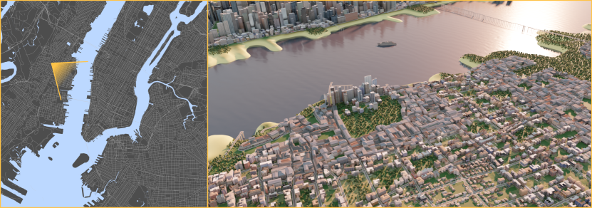
Figure 1. Our system creates diverse street networks at city-scale. Left: A generated layout over an area of 400 km² (20km x 20km) and view frustum (yellow triangle). Right: A rendering of the street graph from the view frustum.

1. Introduction

Generative modeling is an active field of research with many exciting recent contributions. Examples include the generation of realistic human faces using the StyleGAN architecture (Karras et al., 2020, 2021) and the synthesis of images from language prompts (Ramesh et al., 2021, 2022). The goal of this work is to explore the generative modeling of embedded graphs. In particular, we focus on embedded street graphs where each vertex is associated with a 2D coordinate.

We improve on a body of existing work in generative modeling; a typical example of which is Neural Turtle Graphics (Chu et al., 2019), which gives high-quality results for small regions using GRU cells (Li et al., 2016). However, our analysis shows three shortcomings of this work that we address. First, the approach has an inherent limitation in that it encodes and processes graphs as a collection of polylines rather than considering all relevant information (e.g., patterns in the local neighborhood). Even locally, the model does not have a full understanding of its neighborhood. Second, the approach is limited to small areas; for city-scale street networks it is important to scale up the area generated by at least two orders of magnitude. Third, GRU cells have been surpassed by contemporary state-of-the-art generative models, suggesting that more recent approaches may produce stronger results. To overcome these limitations, we propose the following ideas.

Figure 2. We leverage a VQVAE to obtain a context-rich dictionary. A transformer decoder referred to as the IndexModel is trained to learn a conditional prior of the index distribution. The decoder part of the VQVAE together with a thinning and graph tracing approach proposed in (Bastani et al., 2018) is used to obtain a traversable graph.

First, instead of GRU cells we use a transformer architecture (Vaswani et al., 2017) which is a state-of-the-art architecture for generative modeling. Second, we build on auto-regressive models that operate in a compressed space computed by trainable vector quantization (van den Oord et al., 2017). Working in a compressed space provides better scalability of the model since a large-scale transformer architecture is very hard to train and requires a significant amount of hardware. Third, we use a CNN-based decoder to decompress such a quantized representation into an image-based representation. Finally, we use a thinning approach together with the road-tracing approach proposed in (Bastani et al., 2018) to obtain a street graph. Fourth, we employ a combination of sliding window generation and decoding together with conditioning to generate coherent large-scale results. A standard sliding window approach alone would lead to incoherent results. An overview of our architecture is shown in Figure 2.

In summary, our paper contributes a large-scale modeling framework for high-quality street networks that is able to generate street networks that are two orders of magnitude larger than previous generative models for 2D embedded graphs including street graphs.

2. Related Work

2.1. Classical Approaches

Street networks form a key element of generating urban environments. Traditional modeling approaches have been largely procedural or rule-based. This cross-disciplinary area has been surveyed by a number of papers from graphics (Smelik et al., 2014; Kim et al., 2018; Vanegas et al., 2010), architecture (Spencer, 2009), and physics (Barthélemy, 2011).

Procedural Modeling. Müller et al. (Parish and Müller, 2001) introduced a novel self-sensitive L-System (Prusinkiewicz, 1986) which was well suited to the construction of a variety of different street patterns. It has also been adapted by follow up work (Beneš et al., 2011; Kelly and McCabe, 2007). Other approaches include simple grids (Greuter et al., 2003), mesh-based deformable templates (Peng et al., 2014) and hierarchical domain splitting (Yang et al., 2013). Outside of cities, the interaction of street networks with terrain and natural features (e.g., rivers and lakes) are important to generation (Emilien et al., 2012; Galin et al., 2010). One may also apply optimization and simulation in other ways, such as agent-based generation (Song and Whitehead, 2019), or quality of life factors (e.g., daylight or distance to the nearest park) (Vanegas et al., 2012).

Simulation. Street networks are shaped by complex sociological, economic, and technological aspects throughout history. A large body of work studies land use modeling (Lechner et al., 2006) and other work aims to create more accurate street- and city-scapes by simulation over time, in both contemporary (Weber et al., 2009) or historically (Mas et al., 2020) contexts. Given two historical city maps, Krecklau et al. create a smooth animation  (Krecklau et al., 2012) showing city growth over time, while Vanegas et al. create realistic satellite images form such a prediction (Vanegas et al., 2009). Another approach is to allow the user to author a timeline (Williams and Headleand, 2017), which is used to simulate the history of the urban area.

Interactive Techniques. Direct authoring of street network graphs, placing junctions (nodes) and streets (edges) is accurate, but highly time consuming. At the other extreme, geospatial databases (Sun et al., 2002) are accurate and fast, but cannot synthesize novel areas. In between these extremes, interactive authoring of street networks often focuses on higher level primitives, such as tensor fields  (Chen et al., 2008), brushing elements onto existing street networks (Emilien et al., 2015), or street density and patterns (Galin et al., 2011). The recombination of patches of street networks has been investigated using interactive tools such as expand, scale, replace (Aliaga et al., 2008), blending, warping, growing (Nishida et al., 2016), or shrinking street network patches (Pueyo et al., 2020).

2.2. Generative Models

VAEs. The standard VAE (Kingma and Welling, 2014) is an encoder-decoder framework, where the data is encoded into latent variables, and decoded from those latents. Further refinements include more expressive priors (Tomczak and Welling, 2018; Kingma et al., 2016; Chen et al., 2016), or better architectures (Vahdat and Kautz, 2020; Maaløe et al., 2019; Ranganath et al., 2016; Sønderby et al., 2016) which are often hierarchical. VQVAE (van den Oord et al., 2017; Razavi et al., 2019) introduced vector quantization (Gersho and Gray, 1991) to generative models. During training, the latents from the encoder are replaced by their closest element from a learned dictionary. A discrete dictionary works well in conjunction with auto-regressive models based on transformers.

Transformers. The transformer architecture (Vaswani et al., 2017) originally arose in the field of Natural Language Processing but has since been adapted in fields as diverse as object detection (Carion et al., 2020; Beal et al., 2020), image classification (Dosovitskiy et al., 2021), image generation (Parmar et al., 2018; Esser et al., 2020) and layout generation (Para et al., 2020; Wang et al., 2020). A transformer is composed of multiple layers of attention blocks (Parikh et al., 2016; Lin et al., 2017) which model attention over different positions in the sequence. Transformers used as generative models are Auto-Regressive Models (Oord et al., 2016b; Esser et al., 2020) where the generation process occurs step-by-step and the current element depends only on the previously generated elements.

2.3. Graph Synthesis Models

Modeling Graph Connectivity. Deep-generative models for graph-structured data were originally proposed in (Kusner et al., 2017). This was followed by a follow-up work (Dai et al., 2018; Guimaraes et al., 2017; Li et al., 2018; You et al., 2018; De Cao and Kipf, 2018; Simonovsky and Komodakis, 2018) which showed impressive results for molecule generation. Recent methods focus on attaining better performance by using improved architectures (Liao et al., 2019; Li et al., 2021), handling larger graphs by exploiting sparsity (Dai et al., 2020), or improving priors (Shi* et al., 2020; Zang and Wang, 2020; Honda et al., 2020) with flows. Single step generation with VAEs/GANs (De Cao and Kipf, 2018; Simonovsky and Komodakis, 2018), while faster than auto-regressive models (Grover et al., 2019; You et al., 2018; Liao et al., 2019), tends to be of lower quality. These methods are used in domains where nodes do not carry any spatial information and mostly focus on generating valid topology. In the street domain, generating both valid geometry and valid topology is required.

Graphs With Geometric Data. Neural Turtle Graphics (Chu et al., 2019) treats a road network as a graph where the nodes have 2D coordinates. The model is an encoder-decoder architecture based on GRU (Cho et al., 2014) cells in a similar way to Recursive Neural Networks (RNN). For each node, the encoder encodes all the paths which terminate at the node into a hidden state. The decoder works recursively to decode the hidden state into a variable length sequence containing coordinates of the current node, and coordinates of a variable number of neighbouring nodes. PolyGen (Nash et al., 2020) is a method for generating 3D meshes. PolyGen tackles the graph generation problem by factorizing the graph into two models. First a Vertex Model learns the distribution of the nodes/vertices. Second a Face Model learns the connectivity distribution of edges/faces conditioned on the nodes. This enables the modeling of both spatial and topological information. HDMapGen (Mi et al., 2021) also employs auto-regressive modeling for smaller graphs.

We observed that methods like PolyGen (Nash et al., 2020) tend to have problems to provide convincing results when relying on a meaningful topology. We particularly noticed more local errors in connectivity that are ultimately a bit more noticeable than the errors from image-based representations like a distance field. We therefore leverage a robust CNN-based decoder to obtain an image-based representation, followed by a thinning approach and road-tracing method proposed in (Bastani et al., 2018).

Alternatively, GANs could also be used for road modeling (Hartmann et al., 2017; Owaki and Machida, 2020), but it is difficult to compete with auto-regressive models.

3. Methodology

3.1. Overview

Our system consists of multiple parts, an overview of which are introduced in Fig. 2. A graph is traditionally described as $G(V,E)$ where $V$ are the vertices and $E$ the edges; alternatively, graphs can be represented in the image domain by drawing the graph as a 2D image $\mathbf{I}\in\mathbb{R}^{H\times W\times C}$, with $H$ and $W$ being the height and width in pixels respectively and $C$ being the number of color channels, or a distance field of the same resolution. We first learn a compressed representation of the road layout in the image domain by training a single-level VQVAE called the CompressionModel. This gives us an Index Field, $\mathbf{z}_{q}\in\mathbb{Z^{+}}^{H_{q}\times W_{q}}$, which contains indices into a learned dictionary of latents. We experimented with various different image-based representations of a street graph and identified distance fields as giving the best results.

The compressed Index Field representation reduces the sequence length for the decoders which operates on the latent representation. This compression is achieved spatially since $H_{q}<<H$ and $W_{q}<<W$, as well as through the re-use of values in the indexed dictionary. The sliding window generation scheme further limits the effective sequence length, but it requires additional supervision, e.g., in the form of high priority roads, a land water map, and a density map to achieve global consistency. Combining these approaches allows us to model road networks corresponding to over $22km\times 22km$ in the real world, which is over two orders of magnitude larger than prior art. Further, we can achieve this with a transformer, which is otherwise highly sensitive to long sequence lengths.

3.2. Data Preparation

The input to our training procedure are square crops of city areas with each crop being partitioned into a regular grid of equally sized cells. The reasoning behind this partitioning is to have one cell per index to conform to the compression factor of the CompressionModel.

Zoom Level and Projection. We use the Mercator projection for our map data and could identify a crop width of $1223m$ on the equator (zoom level $z=15$ following OpenStreetMap standards) to be a good trade-off between being large enough to show enough spatial context and at the same time being small enough to cause feasible sequence lengths per cell for our transformer models.

Partitioning Into Cells. Each crop is partitioned into a regular grid of $H_{q}\times W_{q}$ equally sized cells to conform to the compression factor of the CompressionModel. In our experiments, we usually choose an input resolution to the CompressionModel of $256\times 256$ pixels and a compression ratio to obtain $16\times 16$ indices as output. Analogously, we subdivide each crop into $16\times 16$ cells which results in an effective cell extent of $76.44m\times 76.44m$.

Density Maps. Our generation is conditioned on a locally computed street density function (street segment length per unit area). The density for each cell is computed at a resolution of $4\times 4$, with each sample’s center over an extent of $1223m\times 1223m$. Computing this map is expensive during test and training time; to this end we accelerate it by pre-computing a global map of densities at a resolution of $76.44m/4=19.11m$. This map may be efficiently convolved for any given sample within a cell to compute the local density.

Street Types. We observed unsatisfying results in early experiments when trying to synthesize a whole street network in one go without distinguishing between the street types (e.g., motorway, residential road); therefore, our goal is to generate a street network in a hierarchical manner by starting with high-priority streets such as highways and to condition the generation of lower-priority streets on already generated streets of higher priority. To this end, we define two priority classes $P_{1}$ and $P_{2}$, with $P_{1}$ being streets of high priority (e.g., motorway, trunk) and $P_{2}$ being streets of low priority (e.g., residential road, living street), and split the data accordingly. For the proof of concept proposed in this paper, we focus on the generation of $P_{2}$ streets and assume an already existing network of $P_{1}$ streets. Please refer to Appendix B for a complete assignment list of street types to priority classes.

Figure 3. Two different image-based representations of an example crop partitioned into $2\times 2$ cells . Left: The crop in the image domain ($32\times 32$ px, $16\times 16$ px per cell) rendered using Bresenham line rasterizer. Right: Distance Field.

3.3. CompressionModel

We leverage the VQGAN implementation of Esser et al. (Esser et al., 2020) to learn a dictionary of context-rich latent codes. However, we could not observe any improvement when using the discriminator $D$ but only use a combination of reconstruction loss, perceptual loss and dictionary loss. Due to this missing adversarial component, we consider our CompressionModel to be a VQVAE. We experimented with a two image-based representations of a street network to be used as input to our model – simple graph drawings and distance fields (See Fig. 3):

Simple Graph Drawings. To represent a graph as a simple image with uniform spatial properties, we draw each edge using a line rasterizer. We use the Bresenham algorithm (Bresenham, 1965) due to its simplicity. However, we observe problems with thin one-pixel-wide edges used as input to the VQVAE – the reconstructions tend to be fragmented and do not retain the important topology of the underlying graph. We therefore experimented with morphological dilation to obtain a better reconstruction quality. This however did not properly solve the mentioned issues. We hypothesize that the VQVAE needs a smooth representation to process information about the street network not only at pixels corresponding to actual elements of the graph, but at each pixel of the input image. This is a condition that a thin rendering does not possess as it has sharp transitions (e.g., between road and non-road regions).

Distance Fields. We use distance fields $\mathcal{D}$ as a smooth image-based representation of the graph. While it would be possible to compute the fields analytically on-demand, we found this to be a performance bottleneck when training. Therefore, we first compute the rasterized graph as a simple graph drawing (as above) and then pre-compute the distance field, interpreting all pixels corresponding to the graph to have a distance of $0$. While this approximation reduces the accuracy of the distance fields, we could not observe a significant drop of the output quality and therefore rasterize all image-based street network data prior to the distance field computation.

3.4. IndexModel

Once we have a trained CompressionModel, we use the model to compress crops from renders of city areas into an index field. We compress into a field having a spatial resolution that is per axis $16$ times smaller than the input resolution. We then train a transformer on this field following (Esser et al., 2020). Our index field is ordered into a sequence $s$. The transformer is trained with the next-token prediction task - given the partial sequence $s_{<i}$, predict the next token. This leads to the following probability model $p(s)=\prod_{i}p(s_{i}|s_{<i})$. Extending the model to generate probabilities, conditioned on a context $c$ (e.g., street density or a land-water map) leads to the following model:

(1) $$p(s)=\prod_{i}p(s_{i}|s_{<i},c)$$

Architecture and Training. The architecture of the transformer is a standard encoder-decoder model, with bidirectional attention on the encoder, and causal attention on the decoder. We use a sliding-window representing the receptive field of the transformer of size $16\times 16$ resulting in a sequence length of $256$. We use a learned positional embedding where the position assigned to each index is the absolute location within the window. We also need to be able to condition on the provided context. There are two forms of context. The first is the cell-based context ($c_{c}$), which is the quantized representation of the density. The density map is $\frac{1}{16}$th the size of the desired spatial resolution of the graph, while $P_{1}$ and the land-water map have the same resolution. The cell-based context is encoded by using a linear layer on the scalar value of the cell to project to the embedding dimension of the transformer. The second type of context is the pixel-based context ($c_{p}$) which is the image based representation of given distance fields (e.g., $P_{1}$ streets) and the land-water map. We extract the patches corresponding to each of the cells in the sliding window from the image representations. The image representations are flattened and projected by a linear layer to the embedding dimension. This is done independently for every cell. The two embedding vectors per-cell are concatenated in the channel dimension, and another linear layer projects them again to the embedding dimension. The encoder input sequence is then the concatenation of all the embedding vectors, this time along the sequence dimension. The complete context $c$, in Eq. 1 is the concatenation of the the two contexts on a per-cell basis $c=[c_{c};c_{p}]$. A transformer encoder encodes this context. A transformer decoder performs cross-attention into the output of the encoder to create a distribution over the possible tokens and generate $s_{i}$ as in Eq. 1.

Inference. In order to generate an index field, we need a set of conditioning maps - a distance field representing $P_{1}$, a density map defining the desired street network density per cell and the land-water map. Inference is almost the same as training, where we take the corresponding crops from the appropriate conditioning maps, move the sliding window by 1 cell during the generation process and denote the generated index field as $\mathcal{F}$. Using the sliding window approach, we are able to generate index fields of arbitrary size. For a street network corresponding to an area of about 20km x 20km, we choose both the height $H_{\mathcal{F}}$ and width $W_{\mathcal{F}}$ of the index field to be 256.

3.5. Decoder

We decode the generated index field $\mathcal{F}$ back into a distance field using the trained decoder of the VQVAE. We post-process the distance field to a graph representation. To do this we first apply a threshold, then using a thinning and road-tracing (Bastani et al., 2018), before finally filtering small disconnected parts. This results in a vector street graph output.

4. Results

We trained on the largest 50 US cities by population to extract a large variety of different city crops. Our results show interesting layouts containing many different patterns.

Implementation Details. Our models are trained on a single node with one to four A100 Nvidia GPUs. For the VQVAE, we use the official VQGAN implementation of (Esser et al., 2020) without a discriminator and the fast transformers library of (Katharopoulos et al., 2020; Vyas et al., 2020) for the IndexModel. For the results shown in this paper, we choose a learning rate of $3.0e-4$, $8$ attention heads, and usually train for $65k$ gradient updates. We found a warm-up of $1k$ gradient updates to be beneficial and use a cosine annealing afterwards. Training takes about $24$ hours for the VQVAE and $48$ hours for the IndexModel. For easier data acquisition, we set up our own OpenStreetMap server consisting of a tile server for the land/water maps and leverage the Overpass API to query the vector data of street networks.

Output Diversity. We use our model repeatedly using the same set of condition maps to show the diversity of the generated results. In Fig. 6, we show two different layouts for crops of size $9.8$ km $\times$ $9.8$ km for three US cities. Note how the model adheres to the given conditions (land/water, higher priority streets, density) to create a different layout in each case.

Large-Scale Results. Using our model in a sliding window fashion we are able to create a city area of arbitrary size. The only limiting factor in this regard is the autoregressive generation which requires the output to be generated sequentially. We validate our system by choosing an area consisting of $256\times 256$ cells, each cell corresponding to an area of about $76$ m $\times$ $76$ m, the output extent thereby corresponding to about $19.5$ km $\times$ $19.5$ km in the Mercator-projected space. Although our system can be used together with a user-defined density map, we use the ground-truth density map for our results to allow a direct comparison with existing cities. In Fig. 1, we show an alternative city layout for New York City. Our model is able to adhere to the provided condition maps in a meaningful way and to generate a diverse layout that would be difficult to achieve with state-of-the-art procedural models.

Style Transfer We experimented with using our trained model to transfer the style of streets between different locations. We used our model that was trained on street patterns in US cities to synthesize street networks for cities in other countries. In Fig. 7 we show the application of the model to recreate Istanbul, in an US style, from high-priority streets, density, and coastline.

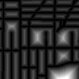
Figure 4. Left: rendered graphs. Right: distance fields.

Comparing Statistics to Procedural Models We use several statistics to compare our results to procedural cities generated by CityEngine (CE). CE has several parameters for street generation, including the pattern type (grid, organic), average block width, and average block length. We estimate these parameters from real cities and compare our generated street networks to CE results. This comparison mainly illustrates that procedural models do not have enough parameters to recreate the pattern of real street maps. We show an example for Chicago in Fig. 8 and more comparisons and an explanation of the statistics in supplementary.

Comparison to GANs.

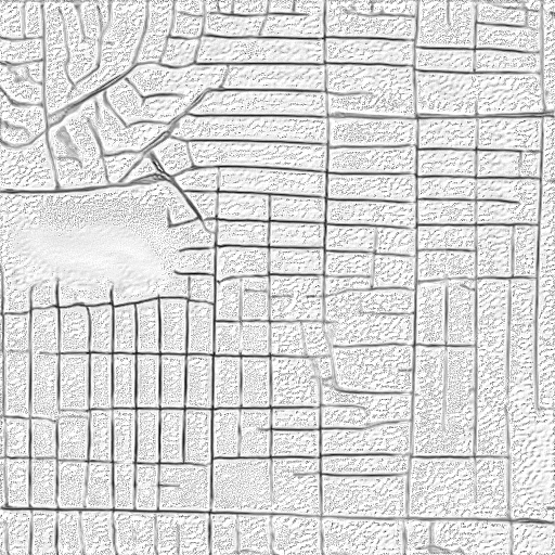
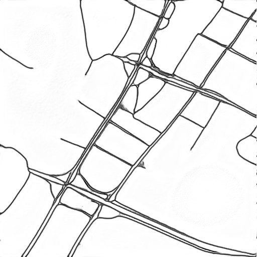
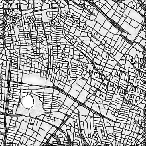
Figure 5. StyleGAN generated image representations of the street network. We found that the output was too noisy (left), did not have enough sharp features (center), or was too different from the training set (right) to create useful street graphs after thinning.

Generative Adversarial Networks (GANs) are another competing approach that could be employed for street generation. We show an example in Fig.5 generated with StyleGANv2 (Karras et al., 2020). While GANs offer the advantage of fast generation times, the output is unusable with the thinning algorithm or other vector graphic extraction algorithms.

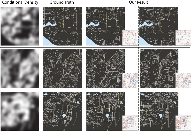
Figure 6. Given the maps for conditioning (land/water, density, existing higher-priority streets), our model is able to generate a large diversity of different street networks. The insets show the difference between the Ground Truth and the generated networks.

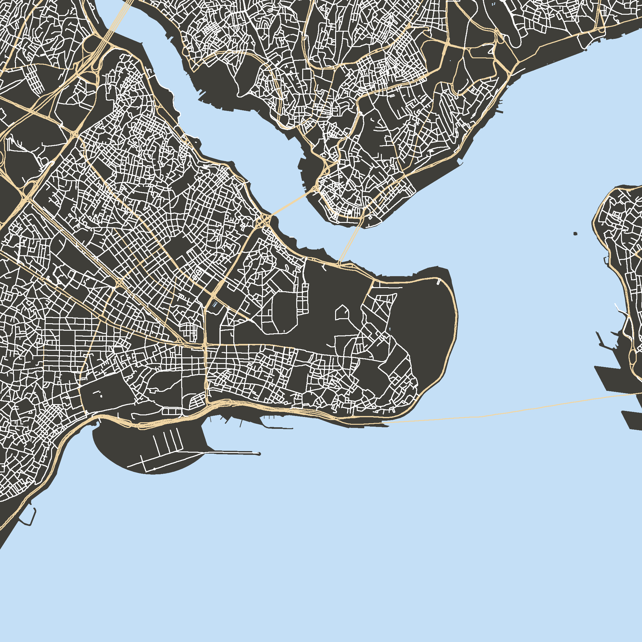
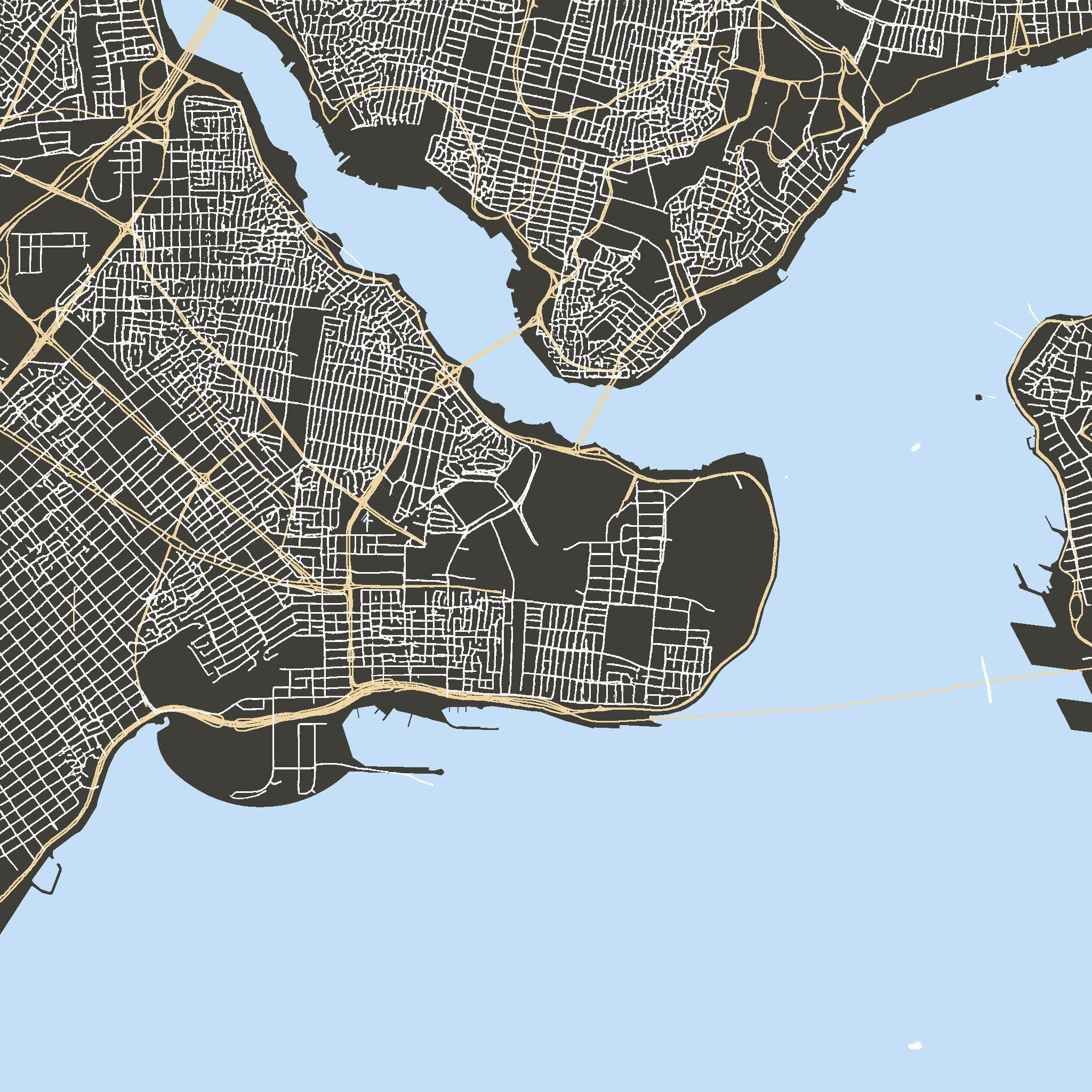
Figure 7. Our model can be used to do style transfer of street pattern. Left: original street map of Istanbul. Right: regenerated street network with the density map of Istanbul by a network trained only on US street graphs.

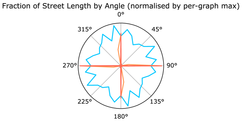
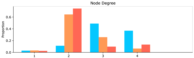
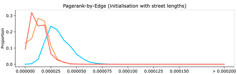
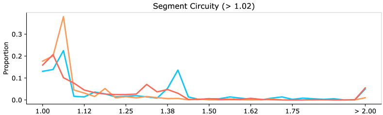
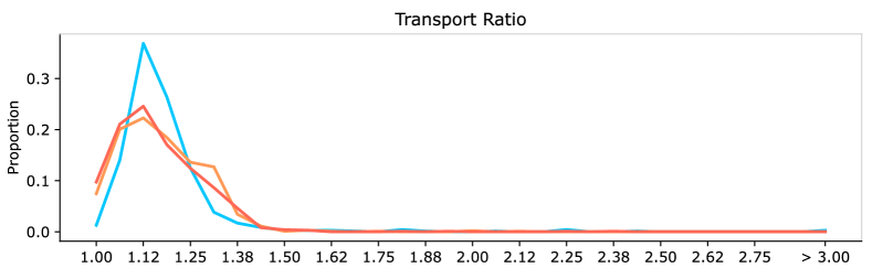
Figure 8. Our model is significantly better able to adhere to statistical numbers of existing cities than the state-of-the art rule-based system CityEngine. Orange: Our model, Red: Ground-Truth, Blue: CityEngine

5. Conclusions, Limitations, and Future Work

We propose a novel framework for modeling large-scale street networks using auto-regressive models. Our results show street networks over two magnitude larger than networks produced by prior art. Our work has some limitations that could be addressed in future work. For now, conditioning information is manually designed. While this provides end-users with control over the generated layouts, it is still a laborious and time consuming process. It would be desirable to generate conditioning information by other generative models specifying only high-level details. Further, we do not consider terrain as conditioning information in the current iteration of the paper. The main reason was the difficulty of obtaining training data. In future work, we hope to expand the model to generate parcels and buildings.

Appendix A Background

There exist many complementary frameworks for generative models - Variational AutoEncoders (VAEs) (Kingma and Welling, 2014), Generative Adversarial Networks (GANs) (Goodfellow et al., 2014), Energy Based Models (EBMs) (Ackley et al., 1987). All of these models can be built using modern building blocks of deep networks - Convolutional Neural Nets (CNNs) (Lecun et al., 1998), transformers (Vaswani et al., 2017) and their numerous variants like UNET (Ronneberger et al., 2015), ResNet (He et al., 2016) for CNNs and Axial Attention (Ho et al., 2020), Longformer (Beltagy et al., 2020) for Transformers.

VAE The standard VAE (Kingma and Welling, 2014) is an encoder-decoder framework, where the data is encoded into latent variables, and decoded from those latents. By making sure that the latents come from a tractable distribution (usually a zero-mean, unit variance Gaussian), efficient sampling is achieved. Further refinements to this base include more expressive priors (Tomczak and Welling, 2018; Kingma et al., 2016; Chen et al., 2016), or better architectures (Vahdat and Kautz, 2020; Maaløe et al., 2019; Ranganath et al., 2016; Sønderby et al., 2016) which are often hierarchical. A complementary strategy to improve performance is to break down training into two steps: 1: autoencoding without any prior; 2: post-hoc learning of the latent. This is the approach adopted by (Ghosh et al., 2020; van den Oord et al., 2017; Razavi et al., 2019).

Specifically, in (van den Oord et al., 2017) the Vector Quantized VAE (VQVAE) is proposed. During training, the latents from the encoder are replaced by their closest element from a learned dictionary, a process known as Vector Quantization in signal processing literature (Gersho and Gray, 1991). As this dictionary has discrete indices, we are therefore able to learn a discrete representation of the input. A prior is then learned over this representation. (Razavi et al., 2019) use a hierarchical version of the VQVAE to model high quality images of up to $1024\times 1024$ pixels.

Transformers The transformer architecture (Vaswani et al., 2017) originally arose in the field of Natural Language Processing, but has since seen prolific use in fields as diverse as Object Detection (Carion et al., 2020; Beal et al., 2020), Image Classification (Dosovitskiy et al., 2021), Image Generation (Parmar et al., 2018; Esser et al., 2020) and Layout Generation (Para et al., 2020; Wang et al., 2020). A transformer is composed of multiple layers of Attention Blocks (Parikh et al., 2016; Lin et al., 2017) which model dependencies of different positions in the sequence relative to each other. Transformers use sequences as their input. Concretely, if we have a sequence $\mathbf{x}=(x_{1},x_{2},\ldots,x_{n})$ of length $n$, we embed these discrete tokens to get the features $X\in\mathbb{R}^{n\times d}$, where $d$ is the dimensionality of the embedding. From this, we compute representations via three independent MLPs and generate query $Q\in\mathbb{R}^{n\times d_{q}}$, key $K\in\mathbb{R}^{n\times d_{q}}$ and value, $V\in\mathbb{R}^{n\times d_{v}}$. The output of the block is then given by

$$\text{Attention}(Q,K,V)=\text{softmax}\left(\frac{QK^{T}}{\sqrt{d_{q}}}\right)V$$

The $n\times n$ matrix, $a_{ij}=\text{softmax}(QK^{T})$ defines the interaction strength between each possible pairs of positions, and uses those as weights to combines the features from $V$. A transformer uses multiple layers of this operation. The matrix formed by the operation $QK^{T}$ has a size $n\times n$ which makes the attention/transformer architecture have an $n^{2}$ dependency on the length of the input sequence. A lot of research has therefore gone into reducing this dependency by using alternative attention schemes.

Auto-Regressive Modelling VAEs focus on decoding latents which are sampled from tractable distributions into entire data points, whether language, images or audio. An alternative to this is to use auto-regressive modelling where the likelihood of data point, say $\mathbf{x}=(x_{1},x_{2},\ldots,x_{n})$ can be decomposed into the product of conditional likelihoods.

$$p(\mathbf{x})=\prod_{i=1}^{n}p(x_{i}|x_{1},x_{2},\ldots,x_{i-1})$$

This is a causal ordering meaning that the probability of the current position depends only on the previously generated positions. This is natural for modalities like language, where words inherently exist in a sequence, but somewhat non-intuitive for images. A simple way to treat the image as a sequence is to flatten the entire $n\times n$ image into a length $n^{2}$ sequence. This is one of the approaches used in (Oord et al., 2016a). In images, where local context is generally more important, a simple modification is possible to save on computation. This modified factorization can be written as

$$p(\mathbf{x})=\prod_{i=1}^{n}p(x_{i}|x_{<i})$$

where $x_{<i}$ refers to any arbitrary subset of pixels before the current pixel. This is usually chosen to be a $k\times k$ causal window around the current pixel which can easily be achieved by Convolutional Networks with proper masking (Salimans et al., 2017; Oord et al., 2016b; Jain et al., 2020).

In the context of transformers, the so-called attention matrix, $a_{ij}=\text{softmax}(QK^{T})$ breaks the causal-ordering by having any position depend on all positions in the sequence. This is fixed by setting $a_{ij}=0$ for the elements where $j\leq i$. With this, the transformer model can only model interactions between elements in the sequence before the current position.

We make heavy use of the VQVAE architecture and an Auto-Regressive transformer in our proposed method.

Appendix B Priority Classes

We use data from the OSM to obtain information about the type of every street. In detail, we extract key-value pairs which are assigned to each way, where a way is what the OSM denotes as a polyline, in our case representing a street section. The key highlighting a way to be a street is the term highway, the value indicates the street type. Note that we do not consider street types like pedestrian ways or street types that do not really contribute to the actual street network of a city like service roads. We assign street sections to the defined priority classes $P_{1}$ and $P_{2}$ according to the values in Table 1.

$P_{1}$	$P_{2}$
motorway	tertiary
trunk	tertiary_link
primary	residential
secondary	living_street
motorway_link	road
trunk_link	unclassified
primary_link
secondary_link

Table 1. Assignment of OSM street types to our three priority classes.

Appendix C L-System streets

Table  2 contains the short and long street length parameters used to generate the street networks. These values were sampled directly from the area in the ground-truth, by computing each block boundary, finding the minimum bounding box, and reporting the short or long length of the box. We took range within one standard deviation of the mean. Following (Parish and Müller, 2001) we used the implementation of CityEngine. An obstacle map was used to mark the water. Following typical street design in North America, major streets followed an organic pattern, and minor streets follow a raster pattern. 50,000 streets were generated and cropped to the region extent. The implementation allowed no control over raster orientation or whether a region bounded by major streets would be filled with minor streets.

	width (m)	deviation	length (m)	deviation
Washington	93.63	93.75	185.48	186.87
Chicago	123.91	96.35	255.29	182.69
Los-Angeles	104.26	86.28	213.58	178.88
San Francisco	96.81	75.98	196.63	159.82
New York	92.97	78.47	182.51	156.60

Table 2. Parameters sampled from the ground-truth used on the L-System streets.

Appendix D Statistical measures

Here we describe the statistical measures used in the evaluation of our networks, but refer the interested reader to  (Boeing, 2020) as an example of the wide area graph statistics in use by the urban planning community.

A segment is a sequence of edges in the graph without branches, connected by vertices with valencies only of 2. circuity measures the ratio between the length of the segment (the sum of the length of the edges in the segment) against the euclidean distance between the first and last vertex of the segment. It describes the local curvature of the streets.

The transport ratio (Boeing, 2019) measures the ratio between the walking distance (along the graph) and the euclidean between two vertices. We sample its value over $n=500$ randomly chosen vertex pairs in the graph. The transport distance describes the connectivity of the city - how easy it is to get between nearby points.

Pagerank is an algorithm originally intended to measure the connectivity of webpages (Page et al., 1999). It has since been applied to the study of street networks (Jiang, 2009), providing a measure of topological connectivity. It models the movements of a traveler through the graph starting from a random vertex, stepping between adjacent vertices randomly, continuing with a probability $k=0.85$ (and halting with a probability $1-k$). As is only a measure of topological connectivity, ignoring vertex position and edge length. To address this, we introduce Pagerank-by-edge. In this model, the traveler travels over an edge graph (EG). An EG has a vertex for every edge in the input graph, and an edge to all adjacent edges in the input graph. We use a $k=0.95$ to simulate longer walks on large graphs. It highlights areas with long edges and high connectivity, at the cost of over-penalizing short edges.

The reported density values normalize the values over the area of land in the street graph. We show all of these statistics in Fig. 9.

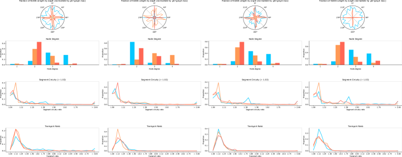
Figure 9. We show statistics from the ground-truth in Red, our model in Orange, and CityEngine in Blue. The cities from left-to-right are Chicago, San Francisco, Washington DC and Los Angeles.

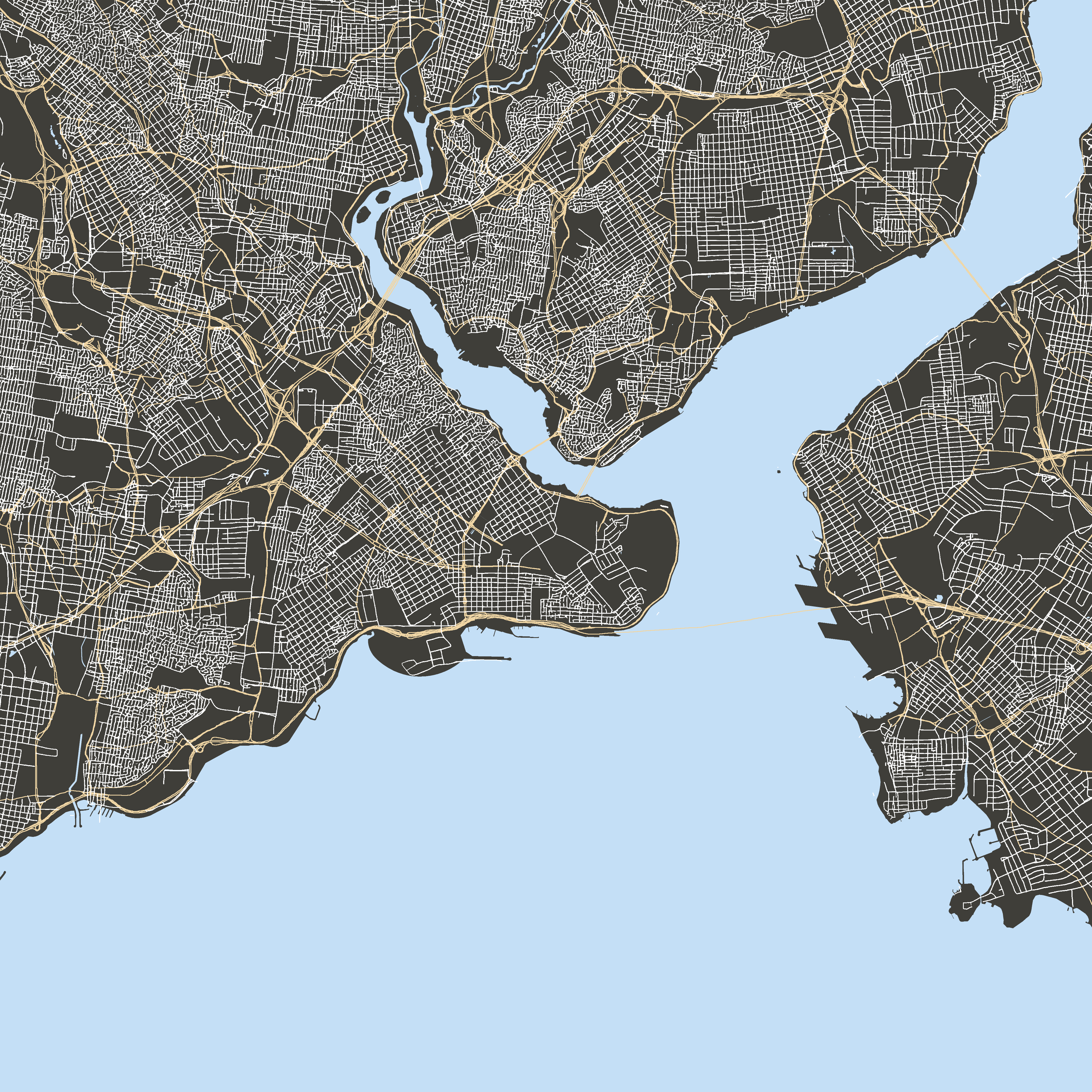
Figure 10. Alternative street layout for the city of Istanbul.

References

- (1)
- Ackley et al. (1987) David Ackley, Geoffrey Hinton, and Terrence Sejnowski. 1987. A Learning Algorithm for Boltzmann Machines. In Readings in Computer Vision, Martin A. Fischler and Oscar Firschein (Eds.). Morgan Kaufmann, San Francisco (CA), 522–533. https://doi.org/10.1016/B978-0-08-051581-6.50053-2
- Aliaga et al. (2008) Daniel G Aliaga, Bedřich Beneš, Carlos A Vanegas, and Nathan Andrysco. 2008. Interactive reconfiguration of urban layouts. IEEE Computer Graphics and Applications 28, 3 (2008), 38–47.
- Barthélemy (2011) Marc Barthélemy. 2011. Spatial networks. Physics Reports 499, 1 (2011), 1–101. https://doi.org/10.1016/j.physrep.2010.11.002
- Bastani et al. (2018) F. Bastani, S. He, S. Abbar, M. Alizadeh, H. Balakrishnan, S. Chawla, S. Madden, and D. DeWitt. 2018. RoadTracer: Automatic Extraction of Road Networks from Aerial Images. In 2018 IEEE/CVF Conference on Computer Vision and Pattern Recognition (CVPR). IEEE Computer Society, Los Alamitos, CA, USA, 4720–4728. https://doi.org/10.1109/CVPR.2018.00496
- Beal et al. (2020) Josh Beal, Eric Kim, Eric Tzeng, Dong Huk Park, Andrew Zhai, and Dmitry Kislyuk. 2020. Toward Transformer-Based Object Detection. arXiv preprint arXiv:2012.09958 (2020).
- Beltagy et al. (2020) Iz Beltagy, Matthew E. Peters, and Arman Cohan. 2020. Longformer: The Long-Document Transformer. ArXiv abs/2004.05150 (2020).
- Beneš et al. (2011) Bedrich Beneš, Ondrej Št’ava, Radomir Měch, and Gavin Miller. 2011. Guided procedural modeling. In Computer Graphics Forum, Vol. 30. Wiley Online Library, 325–334.
- Boeing (2019) Geoff Boeing. 2019. The morphology and circuity of walkable and drivable street networks. In The mathematics of urban morphology. Springer, 271–287.
- Boeing (2020) Geoff Boeing. 2020. A multi-scale analysis of 27,000 urban street networks: Every US city, town, urbanized area, and Zillow neighborhood. Environment and Planning B: Urban Analytics and City Science 47, 4 (2020), 590–608.
- Bresenham (1965) J. E. Bresenham. 1965. Algorithm for computer control of a digital plotter. IBM Systems Journal 4, 1 (1965), 25–30. https://doi.org/10.1147/sj.41.0025
- Carion et al. (2020) Nicolas Carion, Francisco Massa, Gabriel Synnaeve, Nicolas Usunier, Alexander Kirillov, and Sergey Zagoruyko. 2020. End-to-End Object Detection with Transformers. In Computer Vision - ECCV 2020 - 16th European Conference, Glasgow, UK, August 23-28, 2020, Proceedings, Part I (Lecture Notes in Computer Science, Vol. 12346), Andrea Vedaldi, Horst Bischof, Thomas Brox, and Jan-Michael Frahm (Eds.). Springer, 213–229. https://doi.org/10.1007/978-3-030-58452-8_13
- Chen et al. (2008) Guoning Chen, Gregory Esch, Peter Wonka, Pascal Müller, and Eugene Zhang. 2008. Interactive procedural street modeling. ACM Transactions on Graphics (TOG) 27, 3 (2008), 1–10.
- Chen et al. (2016) Xi Chen, Diederik P Kingma, Tim Salimans, Yan Duan, Prafulla Dhariwal, John Schulman, Ilya Sutskever, and Pieter Abbeel. 2016. Variational lossy autoencoder. arXiv preprint arXiv:1611.02731 (2016).
- Cho et al. (2014) Kyunghyun Cho, Bart van Merriënboer, Caglar Gulcehre, Dzmitry Bahdanau, Fethi Bougares, Holger Schwenk, and Yoshua Bengio. 2014. Learning Phrase Representations using RNN Encoder–Decoder for Statistical Machine Translation. In Proceedings of the 2014 Conference on Empirical Methods in Natural Language Processing (EMNLP). Association for Computational Linguistics, Doha, Qatar, 1724–1734. https://doi.org/10.3115/v1/D14-1179
- Chu et al. (2019) Hang Chu, Daiqing Li, David Acuna, Amlan Kar, Maria Shugrina, Xinkai Wei, Ming-Yu Liu, Antonio Torralba, and Sanja Fidler. 2019. Neural Turtle Graphics for Modeling City Road Layouts. In ICCV.
- Dai et al. (2020) Hanjun Dai, Azade Nazi, Yujia Li, Bo Dai, and Dale Schuurmans. 2020. Scalable Deep Generative Modeling for Sparse Graphs. In Proceedings of the 37th International Conference on Machine Learning (Proceedings of Machine Learning Research, Vol. 119), Hal Daumé III and Aarti Singh (Eds.). PMLR, 2302–2312. http://proceedings.mlr.press/v119/dai20b.html
- Dai et al. (2018) Hanjun Dai, Yingtao Tian, Bo Dai, Steven Skiena, and Le Song. 2018. Syntax-Directed Variational Autoencoder for Structured Data. In International Conference on Learning Representations. https://openreview.net/forum?id=SyqShMZRb
- De Cao and Kipf (2018) Nicola De Cao and Thomas Kipf. 2018. MolGAN: An implicit generative model for small molecular graphs. ICML 2018 workshop on Theoretical Foundations and Applications of Deep Generative Models (2018).
- Dosovitskiy et al. (2021) Alexey Dosovitskiy, Lucas Beyer, Alexander Kolesnikov, Dirk Weissenborn, Xiaohua Zhai, Thomas Unterthiner, Mostafa Dehghani, Matthias Minderer, Georg Heigold, Sylvain Gelly, Jakob Uszkoreit, and Neil Houlsby. 2021. An Image is Worth 16x16 Words: Transformers for Image Recognition at Scale. In International Conference on Learning Representations. https://openreview.net/forum?id=YicbFdNTTy
- Emilien et al. (2012) Arnaud Emilien, Adrien Bernhardt, Adrien Peytavie, Marie-Paule Cani, and Eric Galin. 2012. Procedural generation of villages on arbitrary terrains. The Visual Computer 28, 6 (2012), 809–818.
- Emilien et al. (2015) Arnaud Emilien, Ulysse Vimont, Marie-Paule Cani, Pierre Poulin, and Bedrich Benes. 2015. Worldbrush: Interactive example-based synthesis of procedural virtual worlds. ACM Transactions on Graphics (TOG) 34, 4 (2015), 1–11.
- Esser et al. (2020) Patrick Esser, Robin Rombach, and Björn Ommer. 2020. Taming Transformers for High-Resolution Image Synthesis. arXiv:2012.09841 [cs.CV]
- Galin et al. (2011) Eric Galin, Adrien Peytavie, Eric Guérin, and Bedřich Beneš. 2011. Authoring hierarchical road networks. In Computer Graphics Forum, Vol. 30. Wiley Online Library, 2021–2030.
- Galin et al. (2010) E. Galin, A. Peytavie, N. Maréchal, and E. Guérin. 2010. Procedural Generation of Roads. Computer Graphics Forum 29, 2 (2010), 429–438. https://doi.org/10.1111/j.1467-8659.2009.01612.x arXiv:https://onlinelibrary.wiley.com/doi/pdf/10.1111/j.1467-8659.2009.01612.x
- Gersho and Gray (1991) Allen Gersho and Robert M. Gray. 1991. Vector Quantization and Signal Compression. Kluwer Academic Publishers, USA.
- Ghosh et al. (2020) Partha Ghosh, Mehdi S. M. Sajjadi, Antonio Vergari, Michael Black, and Bernhard Scholkopf. 2020. From Variational to Deterministic Autoencoders. In International Conference on Learning Representations. https://openreview.net/forum?id=S1g7tpEYDS
- Goodfellow et al. (2014) Ian Goodfellow, Jean Pouget-Abadie, Mehdi Mirza, Bing Xu, David Warde-Farley, Sherjil Ozair, Aaron Courville, and Yoshua Bengio. 2014. Generative Adversarial Nets. In Advances in Neural Information Processing Systems, Z. Ghahramani, M. Welling, C. Cortes, N. Lawrence, and K. Q. Weinberger (Eds.), Vol. 27. Curran Associates, Inc. https://proceedings.neurips.cc/paper/2014/file/5ca3e9b122f61f8f06494c97b1afccf3-Paper.pdf
- Greuter et al. (2003) Stefan Greuter, Jeremy Parker, Nigel Stewart, and Geoff Leach. 2003. Real-time procedural generation ofpseudo infinite’cities. In Proceedings of the 1st international conference on Computer graphics and interactive techniques in Australasia and South East Asia. 87–ff.
- Grover et al. (2019) Aditya Grover, Aaron Zweig, and S. Ermon. 2019. Graphite: Iterative Generative Modeling of Graphs. ArXiv abs/1803.10459 (2019).
- Guimaraes et al. (2017) G. L. Guimaraes, Benjamín Sánchez-Lengeling, Pedro Luis Cunha Farias, and Alán Aspuru-Guzik. 2017. Objective-Reinforced Generative Adversarial Networks (ORGAN) for Sequence Generation Models. ArXiv abs/1705.10843 (2017).
- Hartmann et al. (2017) Stefan Hartmann, Michael Weinmann, Raoul Wessel, and Reinhard Klein. 2017. Streetgan: Towards road network synthesis with generative adversarial networks. (2017).
- He et al. (2016) Kaiming He, Xiangyu Zhang, Shaoqing Ren, and Jian Sun. 2016. Deep residual learning for image recognition. In Proceedings of the IEEE conference on computer vision and pattern recognition. 770–778.
- Ho et al. (2020) Jonathan Ho, Nal Kalchbrenner, Dirk Weissenborn, and Tim Salimans. 2020. Axial Attention in Multidimensional Transformers. https://openreview.net/forum?id=H1e5GJBtDr
- Honda et al. (2020) Shion Honda, Hirotaka Akita, Katsuhiko Ishiguro, Toshiki Nakanishi, and Kenta Oono. 2020. Graph Residual Flow for Molecular Graph Generation. https://openreview.net/forum?id=SyepHTNFDS
- Jain et al. (2020) Ajay Jain, Pieter Abbeel, and Deepak Pathak. 2020. Locally Masked Convolution for Autoregressive Models. In Conference on Uncertainty in Artificial Intelligence (UAI).
- Jiang (2009) Bin Jiang. 2009. Ranking spaces for predicting human movement in an urban environment. International Journal of Geographical Information Science 23, 7 (2009), 823–837.
- Karras et al. (2020) Tero Karras, Miika Aittala, Janne Hellsten, Samuli Laine, Jaakko Lehtinen, and Timo Aila. 2020. Training Generative Adversarial Networks with Limited Data. In Proc. NeurIPS.
- Karras et al. (2021) Tero Karras, Miika Aittala, Samuli Laine, Erik Härkönen, Janne Hellsten, Jaakko Lehtinen, and Timo Aila. 2021. Alias-Free Generative Adversarial Networks. In NeurIPS.
- Katharopoulos et al. (2020) A. Katharopoulos, A. Vyas, N. Pappas, and F. Fleuret. 2020. Transformers are RNNs: Fast Autoregressive Transformers with Linear Attention. In Proceedings of the International Conference on Machine Learning (ICML).
- Kelly and McCabe (2007) George Kelly and Hugh McCabe. 2007. Citygen: An interactive system for procedural city generation. In Fifth International Conference on Game Design and Technology. 8–16.
- Kim et al. (2018) Joon-Seok Kim, Hamdi Kavak, and Andrew Crooks. 2018. Procedural City Generation beyond Game Development. 10, 2 (nov 2018), 34–41. https://doi.org/10.1145/3292390.3292397
- Kingma et al. (2016) Durk P Kingma, Tim Salimans, Rafal Jozefowicz, Xi Chen, Ilya Sutskever, and Max Welling. 2016. Improved Variational Inference with Inverse Autoregressive Flow. In Advances in Neural Information Processing Systems, D. Lee, M. Sugiyama, U. Luxburg, I. Guyon, and R. Garnett (Eds.), Vol. 29. Curran Associates, Inc. https://proceedings.neurips.cc/paper/2016/file/ddeebdeefdb7e7e7a697e1c3e3d8ef54-Paper.pdf
- Kingma and Welling (2014) Diederik P. Kingma and Max Welling. 2014. Auto-Encoding Variational Bayes. In 2nd International Conference on Learning Representations, ICLR 2014, Banff, AB, Canada, April 14-16, 2014, Conference Track Proceedings, Yoshua Bengio and Yann LeCun (Eds.). http://arxiv.org/abs/1312.6114
- Krecklau et al. (2012) Lars Krecklau, Christopher Manthei, and Leif Kobbelt. 2012. Procedural interpolation of historical city maps. In Computer Graphics Forum, Vol. 31. Wiley Online Library, 691–700.
- Kusner et al. (2017) Matt J. Kusner, Brooks Paige, and José Miguel Hernández-Lobato. 2017. Grammar Variational Autoencoder. In Proceedings of the 34th International Conference on Machine Learning - Volume 70 (Sydney, NSW, Australia) (ICML’17). JMLR.org, 1945–1954.
- Lechner et al. (2006) Thomas Lechner, Pin Ren, Ben Watson, Craig Brozefski, and Uri Wilenski. 2006. Procedural modeling of urban land use. In ACM SIGGRAPH 2006 Research posters. 135–es.
- Lecun et al. (1998) Y. Lecun, L. Bottou, Y. Bengio, and P. Haffner. 1998. Gradient-based learning applied to document recognition. Proc. IEEE 86, 11 (1998), 2278–2324. https://doi.org/10.1109/5.726791
- Li et al. (2021) Jia Li, Jianwei Yu, Da-Cheng Juan, HAN Zhichao, Arjun Gopalan, Hong Cheng, and Andrew Tomkins. 2021. Graph Autoencoders with Deconvolutional Networks. https://openreview.net/forum?id=ohz3OEhVcs
- Li et al. (2018) Yujia Li, Oriol Vinyals, Chris Dyer, Razvan Pascanu, and Peter Battaglia. 2018. Learning Deep Generative Models of Graphs. https://openreview.net/forum?id=Hy1d-ebAb
- Li et al. (2016) Yujia Li, Richard Zemel, Marc Brockschmidt, and Daniel Tarlow. 2016. Gated Graph Sequence Neural Networks. In Proceedings of ICLR’16 (proceedings of iclr’16 ed.). https://www.microsoft.com/en-us/research/publication/gated-graph-sequence-neural-networks/
- Liao et al. (2019) Renjie Liao, Yujia Li, Yang Song, Shenlong Wang, Will Hamilton, David K Duvenaud, Raquel Urtasun, and Richard Zemel. 2019. Efficient Graph Generation with Graph Recurrent Attention Networks. In Advances in Neural Information Processing Systems, H. Wallach, H. Larochelle, A. Beygelzimer, F. d'Alché-Buc, E. Fox, and R. Garnett (Eds.), Vol. 32. Curran Associates, Inc. https://proceedings.neurips.cc/paper/2019/file/d0921d442ee91b896ad95059d13df618-Paper.pdf
- Lin et al. (2017) Zhouhan Lin, Minwei Feng, Cicero Nogueira dos Santos, Mo Yu, Bing Xiang, Bowen Zhou, and Yoshua Bengio. 2017. A structured self-attentive sentence embedding. arXiv preprint arXiv:1703.03130 (2017).
- Maaløe et al. (2019) Lars Maaløe, M. Fraccaro, Valentin Liévin, and O. Winther. 2019. BIVA: A Very Deep Hierarchy of Latent Variables for Generative Modeling. In NeurIPS.
- Mas et al. (2020) Albert Mas, Ignacio Martin, and Gustavo Patow. 2020. Simulating the Evolution of Ancient Fortified Cities. In Computer Graphics Forum, Vol. 39. Wiley Online Library, 650–671.
- Mi et al. (2021) Lu Mi, Hang Zhao, Charlie Nash, Xiaohan Jin, Jiyang Gao, Chen Sun, Cordelia Schmid, Nir Shavit, Yuning Chai, and Dragomir Anguelov. 2021. Hdmapgen: A hierarchical graph generative model of high definition maps. In Proc. CVPR. 4227–4236.
- Nash et al. (2020) Charlie Nash, Yaroslav Ganin, S. M. Ali Eslami, and Peter Battaglia. 2020. PolyGen: An Autoregressive Generative Model of 3D Meshes. In Proceedings of the 37th International Conference on Machine Learning (Proceedings of Machine Learning Research, Vol. 119), Hal Daumé III and Aarti Singh (Eds.). PMLR, 7220–7229. http://proceedings.mlr.press/v119/nash20a.html
- Nishida et al. (2016) Gen Nishida, Ignacio Garcia-Dorado, and Daniel G Aliaga. 2016. Example-driven procedural urban roads. In Computer Graphics Forum, Vol. 35. Wiley Online Library, 5–17.
- Oord et al. (2016a) Aaron Van Oord, Nal Kalchbrenner, and Koray Kavukcuoglu. 2016a. Pixel Recurrent Neural Networks. In Proceedings of The 33rd International Conference on Machine Learning (Proceedings of Machine Learning Research, Vol. 48), Maria Florina Balcan and Kilian Q. Weinberger (Eds.). PMLR, New York, New York, USA, 1747–1756. http://proceedings.mlr.press/v48/oord16.html
- Oord et al. (2016b) Aäron van den Oord, Nal Kalchbrenner, Oriol Vinyals, Lasse Espeholt, Alex Graves, and Koray Kavukcuoglu. 2016b. Conditional Image Generation with PixelCNN Decoders. In Proceedings of the 30th International Conference on Neural Information Processing Systems (Barcelona, Spain) (NIPS’16). Curran Associates Inc., Red Hook, NY, USA, 4797–4805.
- Owaki and Machida (2020) Takashi Owaki and Takashi Machida. 2020. RoadNetGAN: Generating Road Networks in Planar Graph Representation. In International Conference on Neural Information Processing. Springer, 535–543.
- Page et al. (1999) Lawrence Page, Sergey Brin, Rajeev Motwani, and Terry Winograd. 1999. The PageRank citation ranking: Bringing order to the web. Technical Report. Stanford InfoLab.
- Para et al. (2020) Wamiq Para, Paul Guerrero, Tom Kelly, Leonidas Guibas, and Peter Wonka. 2020. Generative Layout Modeling using Constraint Graphs. arXiv preprint arXiv:2011.13417 (2020).
- Parikh et al. (2016) Ankur Parikh, Oscar Täckström, Dipanjan Das, and Jakob Uszkoreit. 2016. A Decomposable Attention Model for Natural Language Inference. In Proceedings of the 2016 Conference on Empirical Methods in Natural Language Processing. Association for Computational Linguistics, Austin, Texas, 2249–2255. https://doi.org/10.18653/v1/D16-1244
- Parish and Müller (2001) Yoav I. H. Parish and Pascal Müller. 2001. Procedural Modeling of Cities. In Proceedings of SIGGRAPH 2001. 301–308. https://doi.org/10.1145/383259.383292
- Parmar et al. (2018) Niki Parmar, Ashish Vaswani, Jakob Uszkoreit, Lukasz Kaiser, Noam Shazeer, Alexander Ku, and Dustin Tran. 2018. Image transformer. In International Conference on Machine Learning. PMLR, 4055–4064.
- Peng et al. (2014) Chi-Han Peng, Yong-Liang Yang, and Peter Wonka. 2014. Computing layouts with deformable templates. ACM Transactions on Graphics (TOG) 33, 4 (2014), 1–11.
- Prusinkiewicz (1986) Przemyslaw Prusinkiewicz. 1986. Graphical applications of L-systems. In Proceedings of graphics interface, Vol. 86. 247–253.
- Pueyo et al. (2020) Oriol Pueyo, Albert Sabrià, Xavier Pueyo, Gustavo Patow, and Michael Wimmer. 2020. Shrinking city layouts. Computers & Graphics 86 (2020), 15–26.
- Ramesh et al. (2022) Aditya Ramesh, Prafulla Dhariwal, Alex Nichol, Casey Chu, and Mark Chen. 2022. Hierarchical Text-Conditional Image Generation with CLIP Latents.
- Ramesh et al. (2021) Aditya Ramesh, Mikhail Pavlov, Gabriel Goh, Scott Gray, Chelsea Voss, Alec Radford, Mark Chen, and Ilya Sutskever. 2021. Zero-Shot Text-to-Image Generation. arXiv:2102.12092 [cs.CV]
- Ranganath et al. (2016) R. Ranganath, Dustin Tran, and D. Blei. 2016. Hierarchical Variational Models. ArXiv abs/1511.02386 (2016).
- Razavi et al. (2019) Ali Razavi, Aaron van den Oord, and Oriol Vinyals. 2019. Generating Diverse High-Fidelity Images with VQ-VAE-2. In Advances in Neural Information Processing Systems, H. Wallach, H. Larochelle, A. Beygelzimer, F. d'Alché-Buc, E. Fox, and R. Garnett (Eds.), Vol. 32. Curran Associates, Inc. https://proceedings.neurips.cc/paper/2019/file/5f8e2fa1718d1bbcadf1cd9c7a54fb8c-Paper.pdf
- Ronneberger et al. (2015) Olaf Ronneberger, Philipp Fischer, and Thomas Brox. 2015. U-Net: Convolutional Networks for Biomedical Image Segmentation. In Medical Image Computing and Computer-Assisted Intervention – MICCAI 2015, Nassir Navab, Joachim Hornegger, William M. Wells, and Alejandro F. Frangi (Eds.). Springer International Publishing, Cham, 234–241.
- Salimans et al. (2017) Tim Salimans, Andrej Karpathy, Xi Chen, and Diederik P. Kingma. 2017. PixelCNN++: A PixelCNN Implementation with Discretized Logistic Mixture Likelihood and Other Modifications. In ICLR.
- Shi* et al. (2020) Chence Shi*, Minkai Xu*, Zhaocheng Zhu, Weinan Zhang, Ming Zhang, and Jian Tang. 2020. GraphAF: a Flow-based Autoregressive Model for Molecular Graph Generation. In International Conference on Learning Representations. https://openreview.net/forum?id=S1esMkHYPr
- Simonovsky and Komodakis (2018) Martin Simonovsky and Nikos Komodakis. 2018. GraphVAE: Towards Generation of Small Graphs Using Variational Autoencoders. https://openreview.net/forum?id=SJlhPMWAW
- Smelik et al. (2014) Ruben M Smelik, Tim Tutenel, Rafael Bidarra, and Bedrich Benes. 2014. A survey on procedural modelling for virtual worlds. In Computer Graphics Forum, Vol. 33. Wiley Online Library, 31–50.
- Sønderby et al. (2016) C. Sønderby, T. Raiko, Lars Maaløe, Søren Kaae Sønderby, and O. Winther. 2016. Ladder Variational Autoencoders. In NIPS.
- Song and Whitehead (2019) Asiiah Song and Jim Whitehead. 2019. TownSim: Agent-based city evolution for naturalistic road network generation. In Proceedings of the 14th International Conference on the Foundations of Digital Games. 1–9.
- Spencer (2009) Douglas Spencer. 2009. Cities and Complexity: Understanding Cities with Cellular Automata, Agent-Based Models, and Fractals. The Journal of Architecture 14, 3 (2009), 446–450. https://doi.org/10.1080/13602360903028044
- Sun et al. (2002) Jing Sun, Xiaobo Yu, George Baciu, and Mark Green. 2002. Template-based generation of road networks for virtual city modeling. In Proceedings of the ACM symposium on Virtual reality software and technology. 33–40.
- Tomczak and Welling (2018) Jakub Tomczak and Max Welling. 2018. VAE with a VampPrior. In Proceedings of the Twenty-First International Conference on Artificial Intelligence and Statistics (Proceedings of Machine Learning Research, Vol. 84), Amos Storkey and Fernando Perez-Cruz (Eds.). PMLR, 1214–1223. http://proceedings.mlr.press/v84/tomczak18a.html
- Vahdat and Kautz (2020) Arash Vahdat and Jan Kautz. 2020. NVAE: A Deep Hierarchical Variational Autoencoder. In Advances in Neural Information Processing Systems, H. Larochelle, M. Ranzato, R. Hadsell, M. F. Balcan, and H. Lin (Eds.), Vol. 33. Curran Associates, Inc., 19667–19679. https://proceedings.neurips.cc/paper/2020/file/e3b21256183cf7c2c7a66be163579d37-Paper.pdf
- van den Oord et al. (2017) Aaron van den Oord, Oriol Vinyals, and koray kavukcuoglu. 2017. Neural Discrete Representation Learning. In Advances in Neural Information Processing Systems, I. Guyon, U. V. Luxburg, S. Bengio, H. Wallach, R. Fergus, S. Vishwanathan, and R. Garnett (Eds.), Vol. 30. Curran Associates, Inc. https://proceedings.neurips.cc/paper/2017/file/7a98af17e63a0ac09ce2e96d03992fbc-Paper.pdf
- Vanegas et al. (2009) Carlos A Vanegas, Daniel G Aliaga, Bedrich Benes, and Paul Waddell. 2009. Visualization of simulated urban spaces: Inferring parameterized generation of streets, parcels, and aerial imagery. IEEE Transactions on Visualization and Computer Graphics 15, 3 (2009), 424–435.
- Vanegas et al. (2010) Carlos A Vanegas, Daniel G Aliaga, Peter Wonka, Pascal Müller, Paul Waddell, and Benjamin Watson. 2010. Modelling the appearance and behaviour of urban spaces. In Computer Graphics Forum, Vol. 29. Wiley Online Library, 25–42.
- Vanegas et al. (2012) Carlos A Vanegas, Ignacio Garcia-Dorado, Daniel G Aliaga, Bedrich Benes, and Paul Waddell. 2012. Inverse design of urban procedural models. ACM Transactions on Graphics (TOG) 31, 6 (2012), 1–11.
- Vaswani et al. (2017) Ashish Vaswani, Noam Shazeer, Niki Parmar, Jakob Uszkoreit, Llion Jones, Aidan N Gomez, Ł ukasz Kaiser, and Illia Polosukhin. 2017. Attention is All you Need. In Advances in Neural Information Processing Systems, I. Guyon, U. V. Luxburg, S. Bengio, H. Wallach, R. Fergus, S. Vishwanathan, and R. Garnett (Eds.), Vol. 30. Curran Associates, Inc. https://proceedings.neurips.cc/paper/2017/file/3f5ee243547dee91fbd053c1c4a845aa-Paper.pdf
- Vyas et al. (2020) A. Vyas, A. Katharopoulos, and F. Fleuret. 2020. Fast Transformers with Clustered Attention. (2020).
- Wang et al. (2020) Xinpeng Wang, Chandan Yeshwanth, and Matthias Nießner. 2020. SceneFormer: Indoor Scene Generation with Transformers. arXiv preprint arXiv:2012.09793 (2020).
- Weber et al. (2009) Basil Weber, Pascal Müller, Peter Wonka, and Markus Gross. 2009. Interactive geometric simulation of 4d cities. In Computer Graphics Forum, Vol. 28. Wiley Online Library, 481–492.
- Williams and Headleand (2017) Benjamin Williams and Christopher J Headleand. 2017. A time-line approach for the generation of simulated settlements. In 2017 International Conference on Cyberworlds (CW). IEEE, 134–141.
- Yang et al. (2013) Yong-Liang Yang, Jun Wang, Etienne Vouga, and Peter Wonka. 2013. Urban pattern: Layout design by hierarchical domain splitting. ACM Transactions on Graphics (TOG) 32, 6 (2013), 1–12.
- You et al. (2018) Jiaxuan You, Rex Ying, Xiang Ren, William L. Hamilton, and Jure Leskovec. 2018. GraphRNN: Generating Realistic Graphs with Deep Auto-regressive Models. In Proceedings of the 35th International Conference on Machine Learning, ICML 2018, Stockholmsmässan, Stockholm, Sweden, July 10-15, 2018 (Proceedings of Machine Learning Research, Vol. 80), Jennifer G. Dy and Andreas Krause (Eds.). PMLR, 5694–5703. http://proceedings.mlr.press/v80/you18a.html
- Zang and Wang (2020) Chengxi Zang and Fei Wang. 2020. MoFlow: An Invertible Flow Model for Generating Molecular Graphs. In Proceedings of the 26th ACM SIGKDD International Conference on Knowledge Discovery; Data Mining (Virtual Event, CA, USA) (KDD ’20). Association for Computing Machinery, New York, NY, USA, 617–626. https://doi.org/10.1145/3394486.3403104