A Bayesian shared-frailty spatial scan statistic model for time-to-event data.

 

Abstract

Spatial scan statistics are well known and widely used methods for the detection of spatial clusters of events. In the field of spatial analysis of time-to-event data, several models of scan statistics have been proposed. However, these models do not take into account the potential intra-unit spatial correlation of individuals nor a potential correlation between spatial units. To overcome this problem, we propose here a scan statistic based on a Cox model with shared frailty that takes into account the spatial correlation between spatial units. In simulation studies, we have shown that (i) classical models of spatial scan statistics for time-to-event data fail to maintain the type I error in the presence of intra-spatial unit correlation, and (ii) our model performs well in the presence of both intra-spatial unit correlation and inter-spatial unit correlation. Our method has been applied to epidemiological data and to the detection of spatial clusters of mortality in patients with end-stage renal disease in northern France.

Keywords: Spatial scan statistics, Time-to-event data, Shared frailty model, Conditional autoregressive model
 

1 Introduction

In many applications, researchers seek to determine if there exist unusual spatial aggregations of data, namely spatial clusters. In the field of public health, epidemiologists seek to identify the presence, within a geographical area, of spatial clusters in which the risk of disease is unusually higher (or lower), thus making it possible to (i) formulate hypotheses to guide etiological research, and (ii) conduct localized public health policies. As another example, in the field of environmental sciences, researchers may be interested in determining the presence of environmental black spots defined by particularly unusual pollutant concentrations in a specific area, thus leading to local actions to prevent or solve the problem.

Among the statistical methods for detecting spatial clusters, spatial scan statistics are widely used methods to detect statistically significant spatial clusters with a scanning window and without any pre-selection bias. These methods were introduced by Kulldorff and Nagarwalla (1995) and Kulldorff (1997) in the cases of Bernoulli and Poisson models. Since then, the approach has been extended to many other spatial data distributions. For example, in the univariate framework, Gaussian (Kulldorff et al., 2009), ordinal (Jung et al., 2007), zero-inflated (Cançado et al., 2014; de Lima et al., 2015; Cançado et al., 2017) and Poisson with overdispersion (Zhang et al., 2012; de Lima et al., 2015) models were proposed. In the context of multivariate or functional data, several spatial scan statistics have also been developed (Kulldorff et al., 2007; Neill and Cooper, 2010; Cucala et al., 2017; Frévent et al., 2021, 2021; Smida et al., 2022). The reader is referred to Abolhassani and Prates (2021) for a more complete review of spatial scan statistics. These methods have been widely used in various fields of application such as epidemiology (Green et al., 2006; Marciano et al., 2018; Genin et al., 2020; Khan et al., 2021), environmental science (Wan et al., 2020; Shi et al., 2021), oncology (Leiser et al., 2020), criminology (Minamisava et al., 2009) and astronomy (De La Fuente Marcos and De La Fuente Marcos, 2008).

In the field of spatial epidemiology, the study of the spatial distribution of time-to-event data can identify areas in which the survival time of patients is different from the rest of the geographical area (e.g., the probability of survival is lower than elsewhere). From an epidemiological point of view, the identification of these areas of unusual survival time is particularly useful to search for local risk factors that condition the survival of patients. Moreover, this information can help public health decision-makers to conduct targeted and specific local policies. In the context of spatial cluster detection of time-to-event data, Huang et al. (2007) and Bhatt and Tiwari (2014) respectively proposed spatial scan statistics based on an exponential and a Weibull model. More recently, Usman and Rosychuk (2018) proposed a parametric model considering a log-Weibull distribution. Although these methods are widely used in practice to detect spatial clusters of time-to-event data (Gregorio et al., 2007; Henry et al., 2009; Wan et al., 2012), they are totally parametric. A first semi-parametric method using a Cox model has been proposed by Cook et al. (2007).

Unlike other spatial scan statistics models, these models consider data measured at the individual level. However, in the field of health data, the exact geographic location of patients is rarely known (i.e., for reasons of anonymity), as patients are rather located through an administrative spatial unit (e.g., municipalities). In this context, the above mentioned methods are based on the strong assumption of independence between observations, which is a classical assumption in the field of spatial scan statistics. This assumption leads to two major drawbacks. First, these methods do not take into account the potential correlation between individuals belonging to the same spatial unit, namely intra-spatial unit correlation. The latter can be induced by unmeasured characteristics of the spatial units (e.g., health care supply) that affect the survival time of patients (Austin, 2017). Second, these methods do not take into account potential spatial correlation between spatial units. However, by nature, spatial data can present a spatial correlation and it is expected that geographically close units are more correlated than distant ones (Li, 2009). Furthermore, it has been shown that ignoring spatial correlation when using spatial scan statistics leads to a significant increase in the type I error (Loh and Zhu, 2007). Since then, several authors have proposed methods that take spatial correlation into account (Loh and Zhu, 2007; Lin, 2014; Lee et al., 2020; Ahmed et al., 2021). However, none of these methods have been designed for time-to-event data and allow for intra-unit spatial correlation.

In the field of time-to-event data analysis, models have been proposed to take into account unobserved factors common to groups of individuals, e.g., members of the same family share a common genetics, patients in the same hospital receive similar care, etc. One way to take into account this intra-group homogeneity is to introduce a random effect common to all individuals in a group, namely shared frailty (Clayton, 1978; Liang et al., 1995; Hougaard, 2000). The shared frailties are assumed to be independent between groups (Liang et al., 1995). However, in the case where the groups correspond to spatial units, such an assumption is unrealistic since close spatial units tend to be correlated (Arlinghaus, 1995). To this end, Li and Ryan (2002) proposed an extension of the shared frailty models to the case of spatially correlated frailty, allowing to take into account not only the intra-spatial unit correlation, but also the possible correlation between the spatial units. This approach has been used in many application studies (Banerjee et al., 2003; Ojiambo and Kang, 2013; Aswi et al., 2020).

This paper develops a new spatial scan statistic for time-to-event data based on a Bayesian semi-parametric Cox model with spatially correlated shared frailties. Section 2 describes the methodological aspects of the scan statistic model. Section 3 proposes both the design and the results of simulation studies that aim at evaluating (i) the performance of classical methods in the presence of intra-unit spatial correlation and (ii) the performance of our approach in the presence of both intra-unit spatial correlation and spatial correlation. Section 4 describes the application of our method to epidemiological data and the detection of spatial clusters of mortality in patients with end-stage renal disease in northern France. Lastly, the results are discussed in Section 5.

2 Methodology

2.1 General principle

Let us consider $K$ non-overlapping spatial locations $s_{1},\dots,s_{k},\dots,s_{K}$ of an observation domain $S\subset\mathbb{R}^{2}$ and $i_{1}^{(k)},\dots,i_{n}^{(k)},\dots,i_{N_{k}}^{(k)}$ be $N_{k}$ individuals belonging to spatial location $s_{k}$. The total number of individuals in $S$ is defined by $N=\sum_{k=1}^{K}N_{k}$. Here we are interested in the time-to-event data measured on individuals: one note respectively $T_{i_{n}^{(k)}}$ and $\delta_{i_{n}^{(k)}}$ the observation time of the $i_{n}$th individual in spatial location $s_{k}$ and $\delta_{i_{n}^{(k)}}$ the censoring indicator which is equal to 0 if the individual $i_{n}^{(k)}$ is censored and 1. In the following, we only consider the cases of right censoring (i.e., the event of interest could not have occurred before the beginning of the study), censoring is assumed to be uninformative, and the event times are supposed to be independent from the censoring times.

We seek to test the presence of spatial clusters in which individuals present shorter (or longer) survival times compared to other individuals observed in the rest of $S$. In this context, spatial scan statistics are designed to detect spatial clusters and to test their statistical significance by testing a null hypothesis $\mathcal{H}_{0}$ (the absence of a cluster) against a composite alternative hypothesis $\mathcal{H}_{1}$ (the presence of at least one cluster $w\subset S$ presenting abnormal time-to-event values). Following Cressie (1977), a spatial scan statistic is the maximum of a concentration index over a set of potential clusters $\mathcal{W}$. In the following and without loss of generality, we focus on variable-size circular clusters. Hence in line with Kulldorff (1997), the set of potential circular clusters $\mathcal{W}$ can be defined by: $\mathcal{W}=\{w_{k,l}/1\leq|w_{k,l}|\leq\frac{N}{2},1\leq k,l\leq K\}$, where $w_{k,l}$ is the disc centred on $s_{k}$ that passes through $s_{l}$ and $|w_{k,l}|$ is the number of individuals in $w_{k,l}$: a cluster comprises at most 50% of the studied population (i.e., $N/2$) (Kulldorff and Nagarwalla, 1995). Remark that in the literature other possibilities have been proposed such as elliptical clusters (Kulldorff et al., 2006), rectangular clusters (Chen and Glaz, 2009) or arbitrarily shaped clusters (Tango and Takahashi, 2005; Zhou et al., 2015; Yin and Mu, 2018).

2.2 Model

We assume that the instantaneous hazard rate at time $t$ for individual $i_{n}^{(k)}$ is

$$\lambda_{i_{n}^{(k)}}(t|\bm{Z}_{i_{n}^{(k)}},\varphi_{k})=\lambda_{0}(t)\exp{\left[\bm{\beta}^{\top}\bm{Z}_{i_{n}^{(k)}}+\varphi_{k}\right]},$$

where $\bm{Z}_{i_{n}^{(k)}}=(Z_{i_{n}^{(k)},1},\dots,Z_{i_{n}^{(k)},p})^{\top}$ is a vector of $p$ covariates associated with the individual $i_{n}^{(k)}$, and $\varphi_{k}$ is the shared frailty associated with the spatial location $s_{k}$. The presence of a spatial cluster in the data results in an effect on the survival times of the spatial units involved. Hence, the effect of this cluster has been incorporated within the shared frailty: for each potential cluster $w$, $\varphi_{k}$ can be decomposed into a cluster effect $\alpha_{w}$ and $X_{k}$ being an effect specific to the spatial location $s_{k}$. Thus, the shared frailties $\varphi_{k}$ associated with the potential cluster $w$ can be rewritten as $\varphi_{k}^{(w)}=\alpha_{w}\mathds{1}_{s_{k}\in w}+X_{k}$ where $\mathbb{E}[X_{k}]=0$. In this context the test hypotheses can be rewritten as $\mathcal{H}_{0}:\forall w\in\mathcal{W},\alpha_{w}=0$ (absence of cluster) and the alternative hypothesis associated with the potential cluster $w$ is $\mathcal{H}_{1}^{(w)}:\alpha_{w}\neq 0$ (presence of a cluster $w$ in which the individuals present atypical survival times).

Moreover, the spatial nature of the data requires taking into account a possible spatial correlation between the different spatial locations $s_{k}$, and thus between the $X_{k}$. This makes it possible to distinguish the effect of the cluster from the spatial correlation of unobserved factors at the scale of the spatial units. Thus, we have considered the Conditional Autoregressive (CAR) model proposed by Leroux et al. (2000) for the distribution of the $X_{k}$:

$$X_{k}|X_{-k}\sim\mathcal{N}\left(\dfrac{\rho\displaystyle\sum_{l=1}^{K}v_{k,l}X_{l}}{\rho\displaystyle\sum_{l=1}^{K}v_{k,l}+1-\rho};\dfrac{\sigma_{X}^{2}}{\rho\displaystyle\sum_{l=1}^{K}v_{k,l}+1-\rho}\right)$$

where $X_{-k}=\{X_{1},\dots,X_{k-1},X_{k+1},\dots,X_{K}\}$, $v_{k,l}=1$ if $s_{k}$ and $s_{l}$ are adjacent (sharing a common boundary) and 0 otherwise, and $\rho\in[0;1]$ is the spatial correlation parameter. It should be noted that if there is no spatial correlation then the $X_{k}$’s are independent and identically distributed (i.i.d.) according to a normal distribution $\mathcal{N}(0,\sigma^{2}_{X})$. Conversely, if $\rho=1$ (i.e., complete spatial correlation between the spatial units) then the $X_{k}$’s are distributed according to an Intrinsic CAR (ICAR) model (Besag et al., 1991).

The proposed method is decomposed into two steps. The first step (Section 2.2.1) consists in estimating the shared frailties $\varphi_{k}$ as well as their spatial correlation parameter $\rho$. In a second step (Section 2.2.2), a scan procedure is developed and applied on the estimated shared frailties to identify spatial clusters of spatial units in which the $\varphi_{k}$ are significantly higher (higher risk) or lower (lower risk) than elsewhere. Lastly, the procedure for determining the statistical significance of the identified spatial clusters is described in Section 2.2.3.

2.2.1 Estimation of the $\varphi_{k}$ and $\rho$

This first step consists in estimating the $\varphi_{k}$ and $\rho$ in a Bayesian framework using the integrated nested Laplace approximation (INLA) (see Rue et al. (2009) for details).

The $\varphi_{k}$ are considered under both the $\mathcal{H}_{0}$ and $\mathcal{H}_{1}$ hypotheses. However, it should be noted that (i) both $X_{k}$ and $\rho$ do not depend on the clustering assumptions as they depend only on the spatial structure of the data and, (ii) only a single vector of $\varphi_{k}$ needs to be estimated in order to best fit the observed data. Therefore, the $\varphi_{k}$ must be estimated under the true hypothesis among $\mathcal{H}_{0}$ and the set of alternative hypotheses $\mathcal{H}_{1}^{(w)}$, i.e., the hypothesis under which the observations have been generated. Following the approach proposed by Ahmed et al. (2021), we need to determine the “best model” among the candidate hypotheses ($\mathcal{H}_{0}$ and $\mathcal{H}_{1}^{(w)}$). For this purpose for each potential cluster $w\in\mathcal{W}$, we considered the Bayes Factor $\text{BF}^{(w)}$, defined as the marginal likelihood ratio between the model under $\mathcal{H}_{1}^{(w)}$ ($\mathcal{M}_{1}^{(w)}$) and the model under $\mathcal{H}_{0}$ ($\mathcal{M}_{0}$):

$$\text{BF}^{(w)}=\dfrac{\mathbb{P}\left[\left\{T_{i_{n}^{(k)}},\delta_{i_{n}^{(k)}},\bm{Z}_{i_{n}^{(k)}},\mathds{1}_{i_{n}^{(k)}\in w}\right\}\big{|}\mathcal{M}_{1}^{(w)}\right]}{\mathbb{P}\left[\left\{T_{i_{n}^{(k)}},\delta_{i_{n}^{(k)}},\bm{Z}_{i_{n}^{(k)}}\right\}\big{|}\mathcal{M}_{0}\right]}.$$

Then, among all the models under $\mathcal{H}_{1}^{(w)}$ we select the “best model” $\mathcal{M}_{1}^{(w^{*})}$ according to this criterion, i.e., the one associated with the potential cluster $w$ maximizing $\text{BF}^{(w)}$. Finally to decide if the estimates should be kept under $\mathcal{H}_{0}$ or under $\mathcal{H}_{1}^{(w^{*})}$, we follow the rule of thumb proposed by Jeffreys (1961): if $\text{BF}^{(w^{*})}\geq 30$ then we keep the estimates (by the posterior mean) under $\mathcal{H}_{1}^{(w^{*})}$, else we keep the estimates (by the posterior mean) under $\mathcal{H}_{0}$. This threshold of 30 corresponds to a “very strong” evidence for $\mathcal{H}_{1}^{(w^{*})}$. Note that if the retained model is $\mathcal{M}_{1}^{(w^{*})}$, the chosen estimate of $\varphi_{k}$ is $\varphi_{k}^{*}=\hat{\alpha}_{w^{*}}\mathds{1}_{s_{k}\in w^{*}}+\hat{X}_{k}$ and if the retained model is $\mathcal{M}_{0}$, $\varphi_{k}^{*}=\hat{X}_{k}$.

2.2.2 Scan procedure

This section develops a scan procedure on the $\varphi_{k}^{*}$ to identify spatial clusters of spatial units in which the $\varphi_{k}^{*}$ are significantly higher (higher risk) or lower (lower risk) than elsewhere. Thus the hypotheses $\mathcal{H}_{0}$ and $\mathcal{H}_{1}^{(w)}$ are redefined in terms of the distribution of the $\varphi_{k}^{*}$ as follows:

$$\mathcal{H}_{0}:\bm{\varphi}^{*}\sim\mathcal{N}(\alpha\mathds{1},\sigma^{2(0)}A^{-1})\text{ and }$$

$$\mathcal{H}_{1}^{(w)}:\bm{\varphi}^{*}\sim\mathcal{N}(\alpha_{w}\mathds{1}_{w}+\alpha_{w^{\mathsf{c}}}\mathds{1}_{w^{\mathsf{c}}},\sigma^{2(w)}A^{-1}),\ \alpha_{w}\neq\alpha_{w^{\mathsf{c}}}$$

where $\bm{\varphi}^{*}=(\varphi_{1}^{*},\dots,\varphi_{K}^{*})^{\top}$, $\mathds{1}$ is the column vector composed only of 1, $\mathds{1}_{w}$ and $\mathds{1}_{w^{\mathsf{c}}}$ are the column indicator vectors of $w$ and $w^{\mathsf{c}}$ respectively, and $A=\rho^{*}R+(1-\rho^{*})\text{I}_{K}$ with $R$ the square matrix composed of the elements

$$R_{k,l}=\left\{\begin{array}[]{ll}\displaystyle\sum_{j=1}^{K}v_{k,j}&\text{ if }k=l\\ -v_{k,l}&\text{ otherwise}\end{array}\right..$$

Note that these assumptions are equivalent to considering both under $\mathcal{H}_{0}$ and $\mathcal{H}_{1}^{(w)}$ the same variance-covariance structure as with the CAR model considered previously (proof in Supplementary Material A), and since $w\cap w^{\mathsf{c}}=\emptyset$, to assume different frailty means in $w$ and $w^{\mathsf{c}}$ under $\mathcal{H}_{1}^{(w)}$ (respectively $\alpha_{w}$ and $\alpha_{w^{\mathsf{c}}}$).

The unknown parameters $\alpha$, $\sigma^{2(0)}$, $\alpha_{w}$, $\alpha_{w^{\mathsf{c}}}$ and $\sigma^{2(w)}$ are estimated by their maximum likelihood estimators (proofs are available in the Appendix B):

$$\hat{\alpha} =\dfrac{\mathds{1}^{\top}A\bm{\varphi}^{*}}{\mathds{1}^{\top}A\mathds{1}},$$

$$\widehat{\sigma^{2(0)}} =\dfrac{1}{K}[\bm{\varphi}^{*\top}A\bm{\varphi}^{*}-2\hat{\alpha}\mathds{1}^{\top}A\bm{\varphi}^{*}+\hat{\alpha}^{2}\mathds{1}^{\top}A\mathds{1}],$$

$$\hat{\alpha}_{w^{\mathsf{c}}} =\left[\mathds{1}_{w^{\mathsf{c}}}^{\top}A\mathds{1}_{w^{\mathsf{c}}}-\dfrac{\mathds{1}_{w}^{\top}A\mathds{1}_{w^{\mathsf{c}}}\mathds{1}_{w}^{\top}A\mathds{1}_{w^{\mathsf{c}}}}{\mathds{1}_{w}^{\top}A\mathds{1}_{w}}\right]^{-1}\left[\mathds{1}_{w^{\mathsf{c}}}^{\top}A\bm{\varphi}^{*}-\dfrac{\mathds{1}_{w}^{\top}A\bm{\varphi}^{*}\mathds{1}_{w}^{\top}A\mathds{1}_{w^{\mathsf{c}}}}{\mathds{1}_{w}^{\top}A\mathds{1}_{w}}\right],$$

$$\hat{\alpha}_{w} =\dfrac{\mathds{1}_{w}^{\top}A\bm{\varphi}^{*}-\hat{\alpha}_{w^{\mathsf{c}}}\mathds{1}_{w}^{\top}A\mathds{1}_{w^{\mathsf{c}}}}{\mathds{1}_{w}^{\top}A\mathds{1}_{w}}\text{ and }$$

$$\widehat{\sigma^{2(w)}} =\dfrac{1}{K}[\bm{\varphi}^{*}-\hat{\alpha}_{w}\mathds{1}_{w}-\hat{\alpha}_{w^{\mathsf{c}}}\mathds{1}_{w^{\mathsf{c}}}]^{\top}A[\bm{\varphi}^{*}-\hat{\alpha}_{w}\mathds{1}_{w}-\hat{\alpha}_{w^{\mathsf{c}}}\mathds{1}_{w^{\mathsf{c}}}].$$

Then the log-likelihood function under $\mathcal{H}_{0}$ has the following expression:

$$\ell_{\mathcal{H}_{0}}(\hat{\alpha},\widehat{\sigma^{2(0)}}) =-\dfrac{K}{2}\ln{[2\pi]}-\dfrac{1}{2}\ln{|A^{-1}|}-\dfrac{K}{2}\ln{[\widehat{\sigma^{2(0)}}]}-\dfrac{K}{2},$$

while the log-likelihood function associated with $\mathcal{H}_{1}^{(w)}$ can be expressed as follows:

$$\ell_{\mathcal{H}_{1}}(\hat{\alpha}_{w},\hat{\alpha}_{w^{\mathsf{c}}},\widehat{\sigma^{2(w)}}) =-\dfrac{K}{2}\ln{[2\pi]}-\dfrac{1}{2}\ln{|A^{-1}|}-\dfrac{K}{2}\ln{[\widehat{\sigma^{2(w)}}]}-\dfrac{K}{2}.$$

Thus the log-likelihood ratio associated with the potential cluster $w$ is

$$LLR^{(w)} =\ell_{\mathcal{H}_{1}}(\hat{\alpha}_{w},\hat{\alpha}_{w^{\mathsf{c}}},\widehat{\sigma^{2(w)}})-\ell_{\mathcal{H}_{0}}(\hat{\alpha},\widehat{\sigma^{2(0)}})$$

$$=\dfrac{K}{2}\left[\ln{\dfrac{\widehat{\sigma^{2(0)}}}{\widehat{\sigma^{2(w)}}}}\right]$$

and finally the spatial scan statistic can be defined as

$$\Lambda=\underset{w\in\mathcal{W}}{\max}\ LLR^{(w)}.$$

The most likely cluster (MLC) is then defined as

$$\text{MLC}=\underset{w\in\mathcal{W}}{\arg\max}\ LLR^{(w)}.$$

2.2.3 Statistical significance

Once the MLC has been detected, its statistical significance must be evaluated. However, the distribution of $\Lambda$ does not have a closed form under $\mathcal{H}_{0}$, so in the literature this distribution is usually approximated by a Monte-Carlo procedure (Dwass, 1957). Two main methods can be distinguished according to the presence (or not) of a distributional hypothesis made on the data. The first method consists in generating data sets under $\mathcal{H}_{0}$, thus requiring a distributional assumption on the data (Kulldorff, 1997). The second method, namely random labelling, consists in randomly permuting the observations among the spatial locations (Kulldorff et al., 2009). In the present case, this method is not applicable because the permutations of the observations do not preserve the spatial correlation of the observations. Therefore, the approximation of the distribution of $\Lambda$ under $\mathcal{H}_{0}$ was performed using the first method: since we have assumed a distribution on the $\varphi_{k}$, one generates $M$ data sets under $\mathcal{H}_{0}$ via $\hat{\alpha}$ and $\widehat{\sigma^{2(0)}}$ which correspond respectively to the estimators of the mean and variance of the $\varphi_{k}$ under $\mathcal{H}_{0}$. For each generated data set $m$, $1\leq m\leq M$, one compute the associated spatial scan statistic $\Lambda^{(m)}$, leading to an approximation of the distribution of $\Lambda$ under $\mathcal{H}_{0}$. Finally, the p-value associated with the MLC is estimated by

$$\hat{p}=\dfrac{1+\displaystyle\sum_{m=1}^{M}\mathds{1}_{\Lambda^{(m)}\geq\Lambda}}{M+1}.$$

3 Simulation studies

Huang et al. (2007) and Cook et al. (2007) proposed spatial scan statistics for time-to-event data indexed in space. However they supposed that the individuals are independent which is a strong and not really realistic hypothesis since individuals located in the same spatial unit can be correlated. Thus, in a first simulation study (Section 3.1), we investigated the impact of the presence of intra-spatial unit correlation on the type I error of the methods proposed by Huang et al. (2007) and Cook et al. (2007).
In Section 3.2, we conducted two simulation studies. The first one (Section 3.2.2) aimed at evaluating the ability of our method to correctly estimate both the spatial correlation parameter and the cluster effect. The second study (Section 3.2.3) aimed, in the presence of spatial correlation, to evaluate the performance of our approach in the context of cluster detection, but also to compare the performance of our method to those of its two particular versions: i.i.d. ($\rho=0$) and ICAR ($\rho=1$).
Lastly, Section 3.3 presents a simulation study that investigated the performance of our approach in the presence of different levels of censoring of time-to-event data.

3.1 Impact of an intra-spatial unit correlation on the type I error of standard methods

In this simulation study, we evaluated the type I errors of classical spatial scan statistics for cluster detection in survival data, namely the exponential model proposed by Huang et al. (2007) and the method based on a log-rank test proposed by Cook et al. (2007), in the presence of an intra-spatial unit correlation.

3.1.1 Design of the simulation

We considered 1690 individuals distributed in 169 spatial units corresponding to administrative subdivisions of northern France, located by their centroid. We defined a spatial cluster $w$ (characterized by $\alpha$) composed of 135 individuals located in 14 contiguous spatial units (the green area on Figure 6 in Supplementary Materials C.1).

We considered the following simulation model: for the individual $i_{n}^{(k)}$ in the spatial unit $s_{k}$,

$$\lambda_{i_{n}^{(k)}}(t|\varphi_{k})=\lambda_{0}(t)\exp{[\varphi_{k}]},$$

with $\lambda_{0}(t)=\frac{1}{2}$ which results in an exponential model. The event times were simulated by the inverse transform sampling: for each individual $i_{n}^{(k)}$, we generated a uniformly distributed random number $u_{i_{n}^{(k)}}$ on $[0;1]$, which allowed to generate a survival time $T_{i_{n}^{(k)}}$ by $T_{i_{n}^{(k)}}=\underset{t>0}{\inf}\ 1-S_{i_{n}^{(k)}}(t)>u_{i_{n}^{(k)}}$. Note that this results in $T_{i_{n}^{(k)}}=-2\ln{[1-u_{i_{n}^{(k)}}]}\exp{[-\varphi_{k}]}$.

The $\varphi_{k}$ were defined by the vector $\bm{\varphi}=(\varphi_{1},\dots,\varphi_{K})^{\top}$ such that

$$\bm{\varphi}\sim\mathcal{N}(\alpha\mathds{1}_{w},\sigma^{2}[\rho R+(1-\rho)I_{K}]^{-1}),$$

where $\mathds{1}_{w}$ is the column indicator vector of $w$.

Here we focused the analysis on the type I errors ($\alpha=0$) of the exponential model (Huang et al., 2007) and the log-rank test method (Cook et al., 2007) in the presence of a non spatially correlated ($\rho=0$) shared frailty for the frailty variance $\sigma^{2}$ varying from 0.001 to 0.101 by increments of 0.010.
For each value of $\sigma^{2}$, 100 data sets were simulated. The statistical significance of the MLC was evaluated as proposed by the authors of the two methods, i.e., by using 999 permutations of the data. The type I error was set to 0.05.

3.1.2 Results

Figure 1 shows the values of the type I error as a function of the values of $\sigma^{2}$. We can notice that the type I error increases when the values of $\sigma^{2}$ increase, showing that the nominal level is not preserved. This can be explained by the fact that, under the hypothesis $\mathcal{H}_{0}$ of absence of cluster, the increase of $\sigma^{2}$ leads directly to the increase of the variance of $X_{k}$. Since the two standard models do not incorporate a shared frailty, the identification of false-positive spatial clusters is essentially due to the intra-unit spatial correlation (i.e, the variance of $X_{k}$).

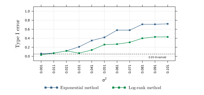
Figure 1: Type I error of the exponential method of Huang et al. (2007) and the log-rank one (Cook et al., 2007) according to the presence of different levels of intra-unit spatial correlation (characterized by the values of the simulated shared frailty variance $\sigma^{2}$).

3.2 Performance evaluation of the proposed method

Here two simulation studies were conducted to evaluate the performance of our approach. The first one (Section 3.2.2) aimed at assessing the ability of our method to accurately estimate both the spatial correlation parameter and the cluster effect. The second study (Section 3.2.3) aimed at evaluating the performance of our method in the context of cluster detection, and comparing it to two particular versions of the model: the one assuming no spatial correlation (i.i.d. frailty model) and the one assuming a complete spatial correlation (ICAR frailty model), in the presence of spatial correlation.

3.2.1 Design of the simulation studies

The design of these simulation studies is very similar to that presented in Section 3.1. The only differences are that since we wanted to investigate the impact of spatial correlation on cluster detection, we set $\sigma^{2}$ to 1 and we considered several values for the parameters controlling the spatial correlation $\rho\in\{0;0.2;0.4;0.6;0.8\}$ and the cluster effect $\alpha\in\{0;0.5;1;1.5;2\}$. Note that $\alpha=0$ was considered to evaluate the maintenance of the type I error.

For each value of the spatial correlation parameter $\rho$ and each value of $\alpha$, 100 data sets were simulated. The statistical significance of the MLC was evaluated through 999 generations of the data under $\mathcal{H}_{0}$ (see Section 2.2.3 for more details) and the type I error was set to 0.05.
The performances were measured through 4 criteria: the power, the true positive rate, the false positive rate and the positive predictive value. The power was estimated as the proportion of simulations leading to the rejection of $\mathcal{H}_{0}$, depending on the type I error. Among the simulated data sets leading to the rejection of $\mathcal{H}_{0}$, the true positive rate was defined as the average proportion of individuals correctly detected among the individuals in $w$, the false positive rate as the average proportion of individuals in $w^{\mathsf{c}}$ that were included in the detected cluster, and the positive predictive value corresponded to the proportion of individuals in $w$ within the detected cluster.

Since the estimations of the $\varphi_{k}$ and $\rho$ were performed in a Bayesian framework, we considered the following Leroux CAR prior for $X_{k}$: $\bm{X}\sim\mathcal{N}(\bm{0},\sigma^{2}[\rho R+(1-\rho)I_{K}]^{-1})$, with a $\bm{\beta}(1;1)$ prior for the spatial correlation parameter $\rho$ and a $\Gamma(10^{-3},10^{-3})$ prior for the precision $1/\sigma^{2}$. For $\alpha_{w}$, we chose a non informative prior $\mathcal{N}(0,10^{3})$.
Lastly, for the baseline hazard $\lambda_{0}$, the observation times were divided into $n_{T}$ time intervals. Here $n_{T}$ was set to be the number of unique times divided by 20. Then, $\lambda_{0}$ was supposed to be constant in each time interval, and for each interval $I$ we supposed $\lambda_{0}=\exp(c_{I})$. We chose a Gaussian prior on the $c_{I}$ increments with precision $\tau$ such that $\tau\sim\Gamma(10^{-3},10^{-3})$: $\Delta c_{I}=c_{I}-c_{I-1}\sim\mathcal{N}(0,\tau^{-1})$.

3.2.2 Evaluation of the estimates of $\rho$ and $\alpha_{w}$

Section 2.2.1 presented the estimation step of the $\varphi_{k}$. Briefly, it consists in choosing either the estimates under the best hypothesis $\mathcal{H}_{1}^{(w)}$: $\mathcal{H}_{1}^{(w^{*})}$ (in this case the estimates are $\varphi_{k}^{*}=\hat{\alpha}_{w^{*}}\mathds{1}_{s_{k}\in w^{*}}+\hat{X}_{k}$) or the estimates under $\mathcal{H}_{0}$ ($\varphi_{k}^{*}=\hat{X}_{k}$). This section focuses on the bias of the estimates obtained for the spatial correlation parameter ($\rho^{*}$), as well as for the cluster effect ($\hat{\alpha}_{w^{*}}$). Note that for the latter we only considered the simulations that did not retain $\mathcal{H}_{0}$ (since otherwise no estimate $\hat{\alpha}_{w^{*}}$ was available). Thus the obtained estimates were compared to the true values of the spatial correlation parameter and the cluster effect.

Figure 2 shows the selected $\rho^{*}$ according to the parameters $\rho$ and $\alpha$ as well as the estimations $\hat{\alpha}_{w^{*}}$ with INLA when we select $\mathcal{H}_{1}$ according to the Bayes Factor criterion.

(a)

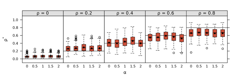
(b)

Figure 2: Simulation study: the selected $\rho^{*}$ according to the parameters $\rho$ and $\alpha$ (panel (a)) and $\hat{\alpha}_{w^{*}}$ obtained with INLA when we select $\mathcal{H}_{1}$ according to the Bayes Factor criterion (panel (b)). The main horizontal lines correspond to the true value of the parameters $\rho$ and $\alpha$ in panels (a) and (b) respectively and the black points represent the mean estimates obtained.

The cluster effect is well estimated by our approach when the simulated values of $\alpha$ are equal to 1, 1.5 and 2. However, it must be pointed that for values of $\alpha$ equal to 0 and 0.5, the cluster effect appears to be poorly estimated. This point arises from the fact that, for these values, our approach rarely selected $\mathcal{H}_{1}$ and, therefore, few estimates were made.

The parameter $\rho$ is globally well estimated although it is slightly overestimated for $\rho=0$ and slightly underestimated for $\rho=0.8$.

3.2.3 Impact of spatial correlation on cluster detection

Here the performance of the proposed method was evaluated in the context of cluster detection. Two particular versions of the method were also considered to investigate the impact of not accounting for spatial correlation although taking into account a potential intra-spatial unit correlation (i.i.d. model, $\rho=0$), or of accounting for it without adjusting its intensity by considering it to be complete (ICAR model, $\rho=1$).

Note that for the ICAR model, $\rho=1$ leads to the non-invertibility of the matrix $A$ and therefore it was not possible to generate data under $\mathcal{H}_{0}$ to estimate the p-value associated with the most likely cluster (see Section 2.2.3 for more details). To overcome this problem,the value of the spatial correlation was fixed at 0.999 instead of 1 in the scan procedure (Section 2.2.2) for the ICAR model.

Figure 3 shows the type I error, the power curves, true positive rates, false positive rates and positive predictive values obtained with our method, as well as with its two special cases: i.i.d. and ICAR.

For the Leroux CAR model, the performances are relatively stable according to the values of $\rho$ although the type I error is slightly higher than the fixed threshold of 5% (except for $\rho=0$ but this is due to the fact that when $\rho=0$, $\rho^{*}$ slightly overestimates $\rho$ (Figure 2) which makes the method quite conservative in this case). Remark that the true and false positive rates and the positive predictive values appear to be less stable according the values of $\rho$ for $\alpha=0.5$. This is due to the fact that these indicators are only computed on the simulations rejecting $\mathcal{H}_{0}$, which are few in this case.

The i.i.d. model fails to maintain a reasonable type I error when $\rho$ increases. Moreover, power according to the values of $\rho$ was less stable than in the CAR model.

The ICAR model tended to absorb the cluster effect in the spatial correlation parameter $\rho$. This is particularly the case when the true value of $\rho$ is low. Thus the type I errors remain reasonable but the power tended to decrease when $\rho$ decreases.

The false positive rates were very low for the three approaches. However, the true positive rates and the positive predictive values were lower for the i.i.d. and the ICAR models than the CAR model.

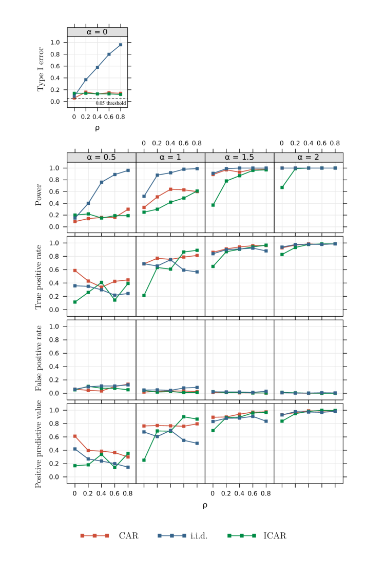
Figure 3: Simulation study: Comparison of the type I error, power curves, true positive and false positive rates and positive predictive values for the CAR, ICAR and i.i.d. models. $\alpha$ is the parameter that controls the cluster intensity and $\rho$ controls the spatial correlation.

Note that the performance of our method was also investigated when considering other thresholds for the Bayes Factor (i.e., 3, 10 and 100 which correspond respectively to “substantial”, “strong” and “decisive” evidences for $\mathcal{H}_{1}^{(w^{*})}$ (Jeffreys, 1961)). The results are presented in Figure 8 in the Appendix C.2.

3.3 Influence of censoring

In this section, a simulation study was conducted to evaluate the performance of our approach in the presence of different levels of censoring in the data.

3.3.1 Design of the simulation

For computational time constraints, the design of the simulation is slightly different from the previous studies: we considered 940 individuals distributed in the 94 French départements located by their centroid. The simulated cluster contains 73 individuals in the 8 départements of Île de France region (see the green area in Figure 7 in Supplementary Materials C.1).

The data were generated in the same way as in Section 3.2 except that a given proportion of observations were censored. In order to simulate different censoring percentages (10%, 20%, 30% and 40%), administrative censoring was considered following Montez-Rath et al. (2017). Briefly, the end of the study was determined so that the right proportion of the observations was censored.

For each value of the spatial correlation parameter $\rho$, each value of $\alpha$, and each censoring percentage, 100 data sets were simulated. The statistical significance of the MLC was evaluated through 999 generations of the data under $\mathcal{H}_{0}$ (see Section 2.2.3 for more details) and the type I error was set to 0.05.
The performances were measured through the same 4 criteria than in Section 3.2: the power, the true positive rate, the false positive rate and the positive predictive value.
Note that in this simulation study the same a priori distributions as in Section 3.2 were considered.

3.3.2 Results

The results of this simulation study are shown in Figure 4. First, we can observe that the power of our method increases when the proportion of censoring increases. This point is also observed for the type I error (see Figure 10 in Supplementary Materials C.3). Although the latter remains stable and close to the nominal type I error (whatever the values of $\rho$) when 10% of the observations are censored, it tends to move away from the nominal type I error as the censoring percentage increases.
False positive rates remain very low regardless of the censoring rate but true positive rates and positive predictive values decrease as the censoring rate increases. However, the impact of censoring on the performance indicators decreases when the intensity $\alpha$ of the cluster increases.

Figure 4: Simulation study: comparison of the power curves, true positive and false positive rates and positive predictive values according to different percentages of censored observations. $\alpha$ is the parameter that controls the cluster intensity and $\rho$ controls the spatial correlation.

4 Application to epidemiological data

4.1 ESRD mortality and related confounding factors

We considered data provided by the French renal epidemiology and information network (REIN) registry on end-stage renal disease (ESRD) in northern France between 2004 and 2020. The methodology of the REIN registry has been described elsewhere (Couchoud et al., 2005). Here, we focused on the analysis of the following endpoint: the mortality measured by the survival time after initiation of dialysis in the population of ESRD patients aged 70 years and older. This population is characterized by (i) a high mortality rate, thus ensuring a high number of observed deaths and, (ii) a low rate of kidney transplantation, thus minimizing the effect of this known competing risk of death among ESRD patients (Hallan et al., 2012; Ayav et al., 2016). The data consist of 6071 individuals for whom the exact time to survival after initiation of dialysis is not known in 17% of cases. These censored observations are either patients still alive at the end of the study (15.7%), or patients lost to follow-up (0.7%), or patients having undergone a renal transplantation (in this case the censoring time corresponds to the date of transplantation) (0.6%). The geographical region studied (northern France, Nord-Pas-de-Calais region) is divided into 80 cantons (a French administrative subdivision) and each individual was associated with a canton, according to his place of residence.

We also considered 18 variables measured at the individual level that are known to be confounders of ESRD patient survival (Couchoud et al., 2015; Fu et al., 2021). Thus, spatial cluster detection was adjusted by introducing the following confounders into each model as covariates: age (in years), sex, body mass index (in $\text{kg/m}^{2}$), type of nephropathy (polycystic, primitive glomerulonephritis, hypertension or vascular, diabetic, pyelonephritis, other), number of cardiovascular comorbidities (none, one, at least two), mobility (autonomous walking, need for a third party, total disability), hemoglobin level (in g/dL), albumin level (in g/dL), dialysis method (haemodialysis or peritoneal dialysis), glomerular filtration rate (below 7, between 7 and 10 or over 10 mL/min/1.73m²), year of treatment initiation (2004-2009, 2010-2015 or 2016-2020), whether or not the treatment was initiated urgently, and the absence or presence of diabete, chronic respiratory disease, respiratory assistance, cirrhosis, severe behavioral disorder and active malignancy. Details of these confounding factors are available in Supplementary Material D.

4.2 Spatial clusters detection

In order to detect spatial clusters of atypical survival times in ESRD patients, 5 models were considered: the exponential model (Model 1) proposed by Huang et al. (2007), the log-rank method proposed by Cook et al. (2007) (Model 2) and the method presented in this paper based on a Cox model considering three types of shared frailty: i.i.d. ($\rho=0$) (Model 3), CAR ($\rho\in]0,1[$) (Model 4) and ICAR ($\rho=1$) (Model 5).

Each model was used to detect spatial clusters of shorter (or longer) survival times compared to the rest of the studied region, among the ESRD patients. To adjust for the confounders in Model 1 we used an exponential regression method to obtain adjusted survival times as proposed by Huang et al. (2007). Regarding Model 2, we followed the approach proposed by Jung (2009); Ahmed and Genin (2020) that consists in estimating the coefficients associated with the confounders in the model under $\mathcal{H}_{0}$ and then fixing their value in the scan statistic proposed by Cook et al. (2007). Regarding Models 3 to 5 (the shared frailty models), we also followed this approach by fixing under each alternative hypothesis $\mathcal{H}_{1}^{(w)}$ the coefficients associated with the confounding factors to their estimated values in the model under $\mathcal{H}_{0}$ in the estimation step of the $\varphi_{k}$ (Section 2.2.1).

In order to provide an indicator of the risk associated with the clusters, which is independent of the model considered, we estimated the Hazard Ratio (HR) associated with each cluster in a classical Cox model adjusted for the confounding factors.

The MLC was considered, together with secondary clusters that had a high value of $\Lambda$ and did not cover the MLC (Kulldorff, 1997). The statistical significance of the detected spatial clusters was evaluated by performing 999 Monte-Carlo simulations, with a type I error of 0.05.

4.3 Results

The spatial clusters detected by each of the 5 models (Exponential, Log-rank, i.i.d., CAR and ICAR frailty) are presented in Figure 5. Detailed information on the spatial clusters is presented in Table 1.

Both the exponential model (Model 1, panel (a) in Figure 5) and the method based on the log-rank test (Model 2, panel (b) in Figure 5) identified the same two statistically significant spatial clusters. The MLC, located in the northeast of the region (green color) presented a close level of significance ($\hat{p}=0.004$ and $\hat{p}=0.005$ respectively) and showed longer survival times than in the rest of the geographical area studied (HR = 0.84 for both models). The first secondary cluster, located in the western part of the region (red color), also had a close level of significance ($\hat{p}=0.025$ and $\hat{p}=0.043$ respectively) and was characterized by shorter survival times (HR=1.13 for both methods).

The i.i.d. frailty model (Model 3, panel (c)) identified the same statistically significant MLC as the exponential model and the method based on the log-rank test ($\hat{p}=0.006$). The CAR (Model 4, panel (d)) and ICAR (Model 5, panel (e)) models both detect the same MLC which contains three more spatial units than the MLC of the other models. It is also characterized by longer survival times (HR=0.86). Although it is statistically significant for the CAR model, it is not statistically significant for the ICAR model ($\hat{p}=0.011$ and $\hat{p}=0.178$ respectively). The first secondary cluster of the three frailty models is the same as the first secondary cluster of the exponential model and the method based on the log-rank test. However it is not statistically significant with the frailty models ($\hat{p}$ = 0.138 for the i.i.d. frailty model, $\hat{p}$ = 0.083 for the CAR frailty model and $\hat{p}$ = 0.949 for the ICAR frailty model respectively).

The small differences between the classical spatial scan statistics methods (Huang et al., 2007; Cook et al., 2007) and the three shared frailty models developed here can be explained by the low variance of the shared frailties (see Figure 11 in Supplementary Materials D for the posterior distribution of $\sigma^{2}$ with each model).

Figure 5: Spatial clusters detected by the method proposed by Huang et al. (2007) (Model 1 (exponential), panel(a)), the method of Cook et al. (2007) (Model 2 (Log-rank), panel (b)) and those highlighted by the shared frailty models (Model 3 (i.i.d.), panel (c); Model 4 (CAR), panel (d); Model 5 (ICAR), panel (e)) after adjusting on confounding factors. Spatial clusters in green indicate longer survival times for ESRD patients compared to the rest of the studied region. Those in red indicate shorter survival times for ESRD patients.

Table 1: Description of the statistically significant spatial clusters detected by the method proposed by Huang et al. (2007) (Model 1 (exponential)), the method of Cook et al. (2007) (Model 2 (Log-rank)) and those detected by the shared frailty models (Model 3 (i.i.d.), Model 4 (CAR) and Model 5 (ICAR)) after adjusting for confounding factors.

Model	Cluster	p-value	Number of	Number of	Number of	Hazard
			spatial units	individuals	events	Ratio1
Model 1	MLC	0.004	10	1091	890	0.84
(Exponential)	Secondary cluster 1	0.025	43	2632	2163	1.13
Model 2	MLC	0.005	10	1091	890	0.84
(Log-rank)	Secondary cluster 1	0.043	43	2632	2163	1.13
Model 3	MLC	0.006	10	1091	890	0.84
(i.i.d. frailty)	Secondary cluster 1	0.138	43	2632	2163	1.13
Model 4	MLC	0.011	13	1346	1094	0.86
(CAR frailty)	Secondary cluster 1	0.083	43	2632	2163	1.13
Model 5	MLC	0.178	13	1346	1094	0.86
ICAR frailty	Secondary cluster 1	0.949	43	2632	2163	1.13

¹ The Hazard Ratio (HR) is computed with a Cox model with adjustment for confounders.

5 Discussion

Here we developed a new spatial scan statistic for survival data indexed in space that allows to take into account both a potential intra-spatial unit correlation and spatial correlation, as well as to adjust the cluster detection on confounding factors. This method is based on a Cox model that includes a spatially structured shared frailty distributed according to a Leroux CAR model.

In a simulation study we showed that, in the presence of intra-spatial unit correlation, the existing methods (Cook et al., 2007; Huang et al., 2007) face a huge increase of the type I error. Thereafter, the performance of the CAR model was evaluated in the context of cluster detection and compared to two particular versions of the latter: the i.i.d. frailty model and the ICAR frailty model. The CAR model presented the best performances in presence of spatial correlation, thus demonstrating a good quality of adjustment of this model on the latter. In a last simulation study, we have shown that the performance of the CAR model remains correct when the percentage of censored observations does not exceed 20%.

These approaches were then applied to epidemiological data to detect the presence of clusters of abnormally low or high survival times in ESRD elderly patients in northern France during the period from 2004 to 2020. The classical approaches (Cook et al., 2007; Huang et al., 2007) detected two statistically significant clusters: one in the northeast of the region corresponding to higher survival times (lower risk) and the other containing the whole western part of the region corresponding to lower survival times (higher risk) than elsewhere. The i.i.d. shared frailty model detected only as statistically significant the cluster in the northeast of the region. Assuming a complete spatial correlation (ICAR model), the method also identified a MLC in the northeast of the region but this latter was not statistically significant. When we considered the CAR frailty model allowing a flexibility of the spatial correlation, a statistically significant cluster was detected in the northeast of the region with a p-value slightly higher than the one provided by the i.i.d. shared frailty model. This can be explained by the consideration by the CAR model of the spatial correlation. These results are consistent with those of the simulation study.

In both the simulation study and the application, circular potential clusters have been considered. However, other cluster shapes (e.g., elliptical clusters (Kulldorff et al., 2006)) could be considered, as the shape of the scanning window has an impact on the power of the method in cluster detection. It should be noted that the choice of another form of scanning window can be easily implemented in our method because it only changes the set of potential clusters $\mathcal{W}$.

In the application on epidemiological data of elderly patients with ESRD, it was observed a low percentage of patients who received a renal transplant. However, this percentage is higher in the general population (Couchoud et al., 2015). It is well known that renal transplantation is a competing risk of death in patients with ESRD, and its non-consideration in the analysis may lead to a biased estimate of the survival function (Hallan et al., 2012). In this context, the proposed method should be modified to account for competing risks by considering, for example, the model proposed by Fine and Gray (1999).

Here the spatial correlation parameter $\rho$ was assumed to be constant over the whole study area. This assumption may be too simplistic because this coefficient may vary spatially (Crawford, 2009). The integration of a spatial correlation coefficient that can vary spatially appears challenging because it is necessary to clearly distinguish the effect of spatial correlation from the effects of spatial clusters present in the data. Adapting the proposed method to this context may be the subject of future work.

In our model, we have included the covariates as fixed effects. However, it is possible to consider them as random effects that may have a spatial correlation. One way to take into account these spatially structured effects is to use conditional autoregressive models for the prior distributions of the coefficients associated with the covariates.

Lastly, our spatial scan statistic can be extended to deal with recurrent events. For example, one may be interested in the time until asthma attack in patients treated for asthma: a patient may experience several asthma attacks during the study period. One possible approach is to consider a shared frailty at the individual level, making it possible to take into account unobserved subject-specific factors (Kleinbaum and Klein, 2012). However, the time to asthma attack may also exhibit an intra-spatial unit correlation (due to environmental factors for example). In this context, one approach would be to consider a nested frailty model (Rondeau, 2010), i.e., a model with both shared frailties at the level of spatial units with a potential spatial correlation, and shared frailties at the level of individuals, in order to take into account both unobserved factors specific to spatial units (e.g., air quality), and unobserved factors specific to individuals (e.g., their tobacco consumption).

Appendix A Leroux prior

The Leroux CAR prior is defined by

$X_{k}|X_{-k}\sim\mathcal{N}\left(\dfrac{\rho\displaystyle\sum_{l=1}^{K}v_{k,l}X_{l}}{\rho\displaystyle\sum_{l=1}^{K}v_{k,l}+1-\rho};\dfrac{\sigma_{X}^{2}}{\rho\displaystyle\sum_{l=1}^{K}v_{k,l}+1-\rho}\right)$ where $v_{k,l}$=1 if $s_{k}$ and $s_{l}$ are adjacent and 0 otherwise.
Let us show (Besag (1974)) that this is equivalent to $\bm{X}\sim\mathcal{N}(0,\sigma^{2}_{X}[\rho R+(1-\rho)I_{K}]^{-1})$, where $R_{k,l}=\left\{\begin{array}[]{ll}\displaystyle\sum_{j=1}^{K}v_{k,j}&\text{ if }k=l\\ -v_{k,l}&\text{ otherwise}\end{array}\right.$,

by applying Brook’s lemma (Brook (1964)) on $\bm{X}$:

$$\dfrac{\mathbb{P}(\bm{X})}{\mathbb{P}(\bm{0})} =\displaystyle\prod_{k=1}^{K}\dfrac{\mathbb{P}(X_{k}|X_{1},\dots X_{k-1},0_{k+1},\dots,0_{K})}{\mathbb{P}(0_{k}|X_{1},\dots X_{k-1},0_{k+1},\dots,0_{K})}.$$

Let $a_{k}$ and $b_{k,l}$ be defined as $a_{k}=\dfrac{\sigma_{X}^{2}}{\rho\displaystyle\sum_{j=1}^{K}v_{k,j}+1-\rho}$ and $b_{k,l}=\dfrac{v_{k,l}}{\rho\displaystyle\sum_{j=1}^{K}v_{k,j}+1-\rho}$, then

$$\dfrac{\mathbb{P}(\bm{X})}{\mathbb{P}(\bm{0})} =\displaystyle\prod_{k=1}^{K}\dfrac{\exp{\left[-\dfrac{1}{2a_{k}}\left(X_{k}-\rho\displaystyle\sum_{l=1}^{k-1}b_{k,l}X_{l}\right)^{2}\right]}}{\exp{\left[-\dfrac{1}{2a_{k}}\left(0_{k}-\rho\displaystyle\sum_{l=1}^{k-1}b_{k,l}X_{l}\right)^{2}\right]}}$$

$$=\displaystyle\prod_{k=1}^{K}\exp{\left[-\dfrac{1}{2a_{k}}\left(X_{k}^{2}-2\rho\displaystyle\sum_{l=1}^{k-1}b_{k,l}X_{k}X_{l}\right)\right]}$$

$$=\displaystyle\prod_{k=1}^{K}\exp{\left[-\dfrac{1}{2\sigma_{X}^{2}}(\rho R_{k,k}+1-\rho)\left(X_{k}^{2}+2\rho\displaystyle\sum_{l=1}^{k-1}\dfrac{R_{k,l}}{\rho R_{k,k}+1-\rho}X_{k}X_{l}\right)\right]}$$

$$=\displaystyle\prod_{k=1}^{K}\exp{\left[-\dfrac{1}{2\sigma_{X}^{2}}\left((\rho R_{k,k}+1-\rho)X_{k}^{2}+2\rho\displaystyle\sum_{l=1}^{k-1}R_{k,l}X_{k}X_{l}\right)\right]}.$$

Let $A=\rho R+(1-\rho)I_{K}$, then

$$\dfrac{\mathbb{P}(\bm{X})}{\mathbb{P}(\bm{0})} =\displaystyle\prod_{k=1}^{K}\exp{\left[-\dfrac{1}{2\sigma_{X}^{2}}\left(A_{k,k}X_{k}^{2}+2\displaystyle\sum_{l=1}^{k-1}A_{k,l}X_{k}X_{l}\right)\right]}$$

$$=\exp{\left[-\dfrac{1}{2\sigma_{X}^{2}}\left(\displaystyle\sum_{k=1}^{K}A_{k,k}X_{k}^{2}+2\displaystyle\sum_{k=1}^{K}\displaystyle\sum_{l=1}^{k-1}A_{k,l}X_{k}X_{l}\right)\right]}.$$

Moreover,

$$2\displaystyle\sum_{k=1}^{K}\displaystyle\sum_{l=1}^{k-1}A_{k,l}X_{k}X_{l} =\displaystyle\sum_{k=1}^{K}\displaystyle\sum_{l=1}^{k-1}A_{k,l}X_{k}X_{l}+\displaystyle\sum_{k=1}^{K}\displaystyle\sum_{l=1}^{k-1}A_{l,k}X_{k}X_{l}\text{ because }A\text{ is symmetric}$$

$$=\displaystyle\sum_{k=1}^{K}\displaystyle\sum_{l=1}^{k-1}A_{k,l}X_{k}X_{l}+\displaystyle\sum_{l=1}^{K}\displaystyle\sum_{k=l+1}^{K}A_{l,k}X_{k}X_{l}$$

$$=\displaystyle\sum_{k=1}^{K}\displaystyle\sum_{l=1}^{k-1}A_{k,l}X_{k}X_{l}+\displaystyle\sum_{k=1}^{K}\displaystyle\sum_{l=k+1}^{K}A_{k,l}X_{l}X_{k}$$

$$=\displaystyle\sum_{k=1}^{K}\displaystyle\sum_{\begin{subarray}{c}l=1\\ l\neq k\end{subarray}}^{K}A_{k,l}X_{k}X_{l}.$$

So

$$\dfrac{\mathbb{P}(\bm{X})}{\mathbb{P}(\bm{0})} =\exp{\left[-\dfrac{1}{2\sigma_{X}^{2}}\left(\displaystyle\sum_{k=1}^{K}A_{k,k}X_{k}^{2}+\displaystyle\sum_{k=1}^{K}\displaystyle\sum_{\begin{subarray}{c}l=1\\ l\neq k\end{subarray}}^{K}A_{k,l}X_{k}X_{l}\right)\right]}$$

$$=\exp{\left[-\dfrac{1}{2\sigma_{X}^{2}}\displaystyle\sum_{k=1}^{K}\displaystyle\sum_{l=1}^{K}A_{k,l}X_{k}X_{l}\right]}$$

$$=\exp{\left[-\dfrac{1}{2\sigma_{X}^{2}}\bm{X}^{\top}A\bm{X}\right]}.$$

Then $\mathbb{P}(\bm{X})\propto\exp{\left[-\dfrac{1}{2\sigma_{X}^{2}}\bm{X}^{\top}A\bm{X}\right]}$ and we recognize the normal distribution $\mathcal{N}(0,\sigma_{X}^{2}A^{-1})$.

Appendix B Maximum likelihood estimators of $\alpha$, $\sigma^{2(0)}$, $\alpha_{w}$, $\alpha_{w^{\mathsf{c}}}$ and $\sigma^{2(w)}$

B.1 Estimation under $\mathcal{H}_{0}$

Under $\mathcal{H}_{0}$ the likelihood is

$$L_{\mathcal{H}_{0}}=\dfrac{1}{(2\pi)^{K/2}|A^{-1}|^{1/2}\sqrt{\sigma^{2K(0)}}}\exp{\left[-\dfrac{1}{2\sigma^{2(0)}}[\bm{\varphi}^{*}-\alpha\mathds{1}]^{\top}A[\bm{\varphi}^{*}-\alpha\mathds{1}]\right]}.$$

Then the log-likelihood is defined by

$$\ell_{\mathcal{H}_{0}} =-\dfrac{K}{2}\ln{[2\pi]}-\dfrac{1}{2}\ln{|A^{-1}|}-\dfrac{K}{2}\ln{[\sigma^{2(0)}]}-\dfrac{1}{2\sigma^{2(0)}}[\bm{\varphi}^{*}-\alpha\mathds{1}]^{\top}A[\bm{\varphi}^{*}-\alpha\mathds{1}]$$

$$=-\dfrac{K}{2}\ln{[2\pi]}-\dfrac{1}{2}\ln{|A^{-1}|}-\dfrac{K}{2}\ln{[\sigma^{2(0)}]}-\dfrac{1}{2\sigma^{2(0)}}[\bm{\varphi}^{*\top}A\bm{\varphi}^{*}-2\alpha\mathds{1}^{\top}A\bm{\varphi}^{*}+\alpha^{2}\mathds{1}^{\top}A\mathds{1}].$$

$$\dfrac{\partial\ell_{\mathcal{H}_{0}}}{\partial\alpha} =-\dfrac{1}{2\sigma^{2(0)}}[-2\mathds{1}^{\top}A\bm{\varphi}^{*}+2\alpha\mathds{1}^{\top}A\mathds{1}].$$

Thus $\dfrac{\partial\ell_{\mathcal{H}_{0}}}{\partial\alpha}=0\iff\alpha\mathds{1}^{\top}A\mathds{1}=\mathds{1}^{\top}A\bm{\varphi}^{*}\iff\alpha=\dfrac{\mathds{1}^{\top}A\bm{\varphi}^{*}}{\mathds{1}^{\top}A\mathds{1}}$.

$$\dfrac{\partial\ell_{\mathcal{H}_{0}}}{\partial\sigma^{2(0)}} =-\dfrac{K}{2\sigma^{2(0)}}+\dfrac{1}{2\sigma^{4(0)}}[\bm{\varphi}^{*\top}A\bm{\varphi}^{*}-2\alpha\mathds{1}^{\top}A\bm{\varphi}^{*}+\alpha^{2}\mathds{1}^{\top}A\mathds{1}].$$

Then $\dfrac{\partial\ell_{\mathcal{H}_{0}}}{\partial\sigma^{2(0)}}=0\iff\sigma^{2(0)}=\dfrac{1}{K}[\bm{\varphi}^{*\top}A\bm{\varphi}^{*}-2\alpha\mathds{1}^{\top}A\bm{\varphi}^{*}+\alpha^{2}\mathds{1}^{\top}A\mathds{1}]$.

Finally $\hat{\alpha}=\dfrac{\mathds{1}^{\top}A\bm{\varphi}^{*}}{\mathds{1}^{\top}A\mathds{1}}$ and $\widehat{\sigma^{2(0)}}=\dfrac{1}{K}[\bm{\varphi}^{*\top}A\bm{\varphi}^{*}-2\hat{\alpha}\mathds{1}^{\top}A\bm{\varphi}^{*}+\hat{\alpha}^{2}\mathds{1}^{\top}A\mathds{1}]$.

B.2 Estimation under $\mathcal{H}_{1}^{(w)}$

Under $\mathcal{H}_{1}^{(w)}$ the likelihood is

$$L_{\mathcal{H}_{1}^{(w)}}=\dfrac{1}{(2\pi)^{K/2}|A^{-1}|^{1/2}\sqrt{\sigma^{2K(w)}}}\exp{\left[-\dfrac{1}{2\sigma^{2(w)}}[\bm{\varphi}^{*}-\alpha_{w}\mathds{1}_{w}-\alpha_{w^{\mathsf{c}}}\mathds{1}_{w^{\mathsf{c}}}]^{\top}A[\bm{\varphi}^{*}-\alpha_{w}\mathds{1}_{w}-\alpha_{w^{\mathsf{c}}}\mathds{1}_{w^{\mathsf{c}}}]\right]}.$$

Thus the log-likelihood can be computed:

$$\ell_{\mathcal{H}_{1}^{(w)}} =-\dfrac{K}{2}\ln{[2\pi]}-\dfrac{1}{2}\ln{|A^{-1}|}-\dfrac{K}{2}\ln{[\sigma^{2(w)}]}-\dfrac{1}{2\sigma^{2(w)}}[\bm{\varphi}^{*}-\alpha_{w}\mathds{1}_{w}-\alpha_{w^{\mathsf{c}}}\mathds{1}_{w^{\mathsf{c}}}]^{\top}A[\bm{\varphi}^{*}-\alpha_{w}\mathds{1}_{w}-\alpha_{w^{\mathsf{c}}}\mathds{1}_{w^{\mathsf{c}}}]$$

$$=-\dfrac{K}{2}\ln{[2\pi]}-\dfrac{1}{2}\ln{|A^{-1}|}-\dfrac{K}{2}\ln{[\sigma^{2(w)}]}$$

$$\hskip 11.38092pt-\dfrac{1}{2\sigma^{2(w)}}[\bm{\varphi}^{*\top}A\bm{\varphi}^{*}-2\alpha_{w}\mathds{1}_{w}^{\top}A\bm{\varphi}^{*}+\alpha_{w}^{2}\mathds{1}_{w}^{\top}A\mathds{1}_{w}+2\alpha_{w}\alpha_{w^{\mathsf{c}}}\mathds{1}_{w}^{\top}A\mathds{1}_{w^{\mathsf{c}}}-2\alpha_{w^{\mathsf{c}}}\mathds{1}_{w^{\mathsf{c}}}^{\top}A\bm{\varphi}^{*}+\alpha_{w^{\mathsf{c}}}^{2}\mathds{1}_{w^{\mathsf{c}}}^{\top}A\mathds{1}_{w^{\mathsf{c}}}].$$

$$\dfrac{\partial\ell_{\mathcal{H}_{1}^{(w)}}}{\partial\alpha_{w}}=-\dfrac{1}{2\sigma^{2(w)}}[-2\mathds{1}_{w}^{\top}A\bm{\varphi}^{*}+2\alpha_{w}\mathds{1}_{w}^{\top}A\mathds{1}_{w}+2\alpha_{w^{\mathsf{c}}}\mathds{1}_{w}^{\top}A\mathds{1}_{w^{\mathsf{c}}}].$$

Then $\dfrac{\partial\ell_{\mathcal{H}_{1}^{(w)}}}{\partial\alpha_{w}}=0\iff\alpha_{w}\mathds{1}_{w}^{\top}A\mathds{1}_{w}=\mathds{1}_{w}^{\top}A\bm{\varphi}^{*}-\alpha_{w^{\mathsf{c}}}\mathds{1}_{w}^{\top}A\mathds{1}_{w^{\mathsf{c}}}$.

$$\dfrac{\partial\ell_{\mathcal{H}_{1}^{(w)}}}{\partial\alpha_{w^{\mathsf{c}}}}=-\dfrac{1}{2\sigma^{2(w)}}[-2\mathds{1}_{w^{\mathsf{c}}}^{\top}A\bm{\varphi}^{*}+2\alpha_{w^{\mathsf{c}}}\mathds{1}_{w^{\mathsf{c}}}^{\top}A\mathds{1}_{w^{\mathsf{c}}}+2\alpha_{w}\mathds{1}_{w}^{\top}A\mathds{1}_{w^{\mathsf{c}}}].$$

Then $\dfrac{\partial\ell_{\mathcal{H}_{1}^{(w)}}}{\partial\alpha_{w^{\mathsf{c}}}}=0\iff\alpha_{w^{\mathsf{c}}}\mathds{1}_{w^{\mathsf{c}}}^{\top}A\mathds{1}_{w^{\mathsf{c}}}=\mathds{1}_{w^{\mathsf{c}}}^{\top}A\bm{\varphi}^{*}-\alpha_{w}\mathds{1}_{w}^{\top}A\mathds{1}_{w^{\mathsf{c}}}$.

We deduce:

$$\left\{\begin{array}[]{rl}\dfrac{\partial\ell_{\mathcal{H}_{1}^{(w)}}}{\partial\alpha_{w}}&=0\\ \dfrac{\partial\ell_{\mathcal{H}_{1}^{(w)}}}{\partial\alpha_{w^{\mathsf{c}}}}&=0\end{array}\right. \iff\left\{\begin{array}[]{rl}\alpha_{w}\mathds{1}_{w}^{\top}A\mathds{1}_{w}&=\mathds{1}_{w}^{\top}A\bm{\varphi}^{*}-\alpha_{w^{\mathsf{c}}}\mathds{1}_{w}^{\top}A\mathds{1}_{w^{\mathsf{c}}}\\ \alpha_{w^{\mathsf{c}}}\mathds{1}_{w^{\mathsf{c}}}^{\top}A\mathds{1}_{w^{\mathsf{c}}}&=\mathds{1}_{w^{\mathsf{c}}}^{\top}A\bm{\varphi}^{*}-\alpha_{w}\mathds{1}_{w}^{\top}A\mathds{1}_{w^{\mathsf{c}}}\end{array}\right.$$

$$\iff\left\{\begin{array}[]{rl}\alpha_{w}&=\dfrac{\mathds{1}_{w}^{\top}A\bm{\varphi}^{*}-\alpha_{w^{\mathsf{c}}}\mathds{1}_{w}^{\top}A\mathds{1}_{w^{\mathsf{c}}}}{\mathds{1}_{w}^{\top}A\mathds{1}_{w}}\\ \alpha_{w^{\mathsf{c}}}\mathds{1}_{w^{\mathsf{c}}}^{\top}A\mathds{1}_{w^{\mathsf{c}}}&=\mathds{1}_{w^{\mathsf{c}}}^{\top}A\bm{\varphi}^{*}-\dfrac{\mathds{1}_{w}^{\top}A\bm{\varphi}^{*}-\alpha_{w^{\mathsf{c}}}\mathds{1}_{w}^{\top}A\mathds{1}_{w^{\mathsf{c}}}}{\mathds{1}_{w}^{\top}A\mathds{1}_{w}}\mathds{1}_{w}^{\top}A\mathds{1}_{w^{\mathsf{c}}}\end{array}\right.$$

$$\iff\left\{\begin{array}[]{rl}\alpha_{w}&=\dfrac{\mathds{1}_{w}^{\top}A\bm{\varphi}^{*}-\alpha_{w^{\mathsf{c}}}\mathds{1}_{w}^{\top}A\mathds{1}_{w^{\mathsf{c}}}}{\mathds{1}_{w}^{\top}A\mathds{1}_{w}}\\ \alpha_{w^{\mathsf{c}}}&=\left[\mathds{1}_{w^{\mathsf{c}}}^{\top}A\mathds{1}_{w^{\mathsf{c}}}-\dfrac{\mathds{1}_{w}^{\top}A\mathds{1}_{w^{\mathsf{c}}}\mathds{1}_{w}^{\top}A\mathds{1}_{w^{\mathsf{c}}}}{\mathds{1}_{w}^{\top}A\mathds{1}_{w}}\right]^{-1}\left[\mathds{1}_{w^{\mathsf{c}}}^{\top}A\bm{\varphi}^{*}-\dfrac{\mathds{1}_{w}^{\top}A\bm{\varphi}^{*}\mathds{1}_{w}^{\top}A\mathds{1}_{w^{\mathsf{c}}}}{\mathds{1}_{w}^{\top}A\mathds{1}_{w}}\right].\end{array}\right.$$

$$\dfrac{\partial\ell_{\mathcal{H}_{1}^{(w)}}}{\partial\sigma^{2(w)}}=-\dfrac{K}{2\sigma^{2(w)}}+\dfrac{1}{2\sigma^{4(w)}}[\bm{\varphi}^{*}-\alpha_{w}\mathds{1}_{w}-\alpha_{w^{\mathsf{c}}}\mathds{1}_{w^{\mathsf{c}}}]^{\top}A[\bm{\varphi}^{*}-\alpha_{w}\mathds{1}_{w}-\alpha_{w^{\mathsf{c}}}\mathds{1}_{w^{\mathsf{c}}}].$$

Then $\dfrac{\partial\ell_{\mathcal{H}_{1}^{(w)}}}{\partial\sigma^{2(w)}}=0\iff\sigma^{2(w)}=\dfrac{1}{K}[\bm{\varphi}^{*}-\alpha_{w}\mathds{1}_{w}-\alpha_{w^{\mathsf{c}}}\mathds{1}_{w^{\mathsf{c}}}]^{\top}A[\bm{\varphi}^{*}-\alpha_{w}\mathds{1}_{w}-\alpha_{w^{\mathsf{c}}}\mathds{1}_{w^{\mathsf{c}}}].$

Finally $\hat{\alpha}_{w^{\mathsf{c}}}=\left[\mathds{1}_{w^{\mathsf{c}}}^{\top}A\mathds{1}_{w^{\mathsf{c}}}-\dfrac{\mathds{1}_{w}^{\top}A\mathds{1}_{w^{\mathsf{c}}}\mathds{1}_{w}^{\top}A\mathds{1}_{w^{\mathsf{c}}}}{\mathds{1}_{w}^{\top}A\mathds{1}_{w}}\right]^{-1}\left[\mathds{1}_{w^{\mathsf{c}}}^{\top}A\bm{\varphi}^{*}-\dfrac{\mathds{1}_{w}^{\top}A\bm{\varphi}^{*}\mathds{1}_{w}^{\top}A\mathds{1}_{w^{\mathsf{c}}}}{\mathds{1}_{w}^{\top}A\mathds{1}_{w}}\right]$,
$\hat{\alpha}_{w}=\dfrac{\mathds{1}_{w}^{\top}A\bm{\varphi}^{*}-\hat{\alpha}_{w^{\mathsf{c}}}\mathds{1}_{w}^{\top}A\mathds{1}_{w^{\mathsf{c}}}}{\mathds{1}_{w}^{\top}A\mathds{1}_{w}}$ and $\widehat{\sigma^{2(w)}}=\dfrac{1}{K}[\bm{\varphi}^{*}-\hat{\alpha}_{w}\mathds{1}_{w}-\hat{\alpha}_{w^{\mathsf{c}}}\mathds{1}_{w^{\mathsf{c}}}]^{\top}A[\bm{\varphi}^{*}-\hat{\alpha}_{w}\mathds{1}_{w}-\hat{\alpha}_{w^{\mathsf{c}}}\mathds{1}_{w^{\mathsf{c}}}]$.

Appendix C Simulation study

C.1 Design of the simulation study

Figures 6 and 7 show the spatial units as well as the cluster considered in the simulation study in the absence and in the presence of censoring respectively.

Figure 6: Simulated cluster (in green) in 169 administrative subdivisions of northern France.

Figure 7: Simulated cluster (in green) in the 94 départements of France.

C.2 Influence of the threshold chosen for the Bayes Factor

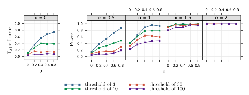
Figure 8: Simulation study: Type I error and power curves depending on the chosen threshold for the Bayes Factor to select the frailty values under $\mathcal{H}_{0}$ or under $\mathcal{H}_{1}^{(w^{*})}$. $\alpha$ is the parameter that controls the cluster intensity and $\rho$ controls the spatial correlation.

Figure 8 shows the type I error and the power curves of the proposed method with several thresholds for the Bayes Factor (3, 10, 30 and 100). The thresholds of 3 and 10 do not maintain a stable type I error according to the values of $\rho$. The threshold of 100 maintains the type I error very well but is very conservative. The threshold of 30 seems to be a good compromise.

However, we decided to investigate whether the estimates of the parameters with a threshold of 100 were better (less biased) than with a threshold of 30. Figure 9 shows that this is not the case.

(a)

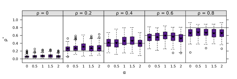
(b)

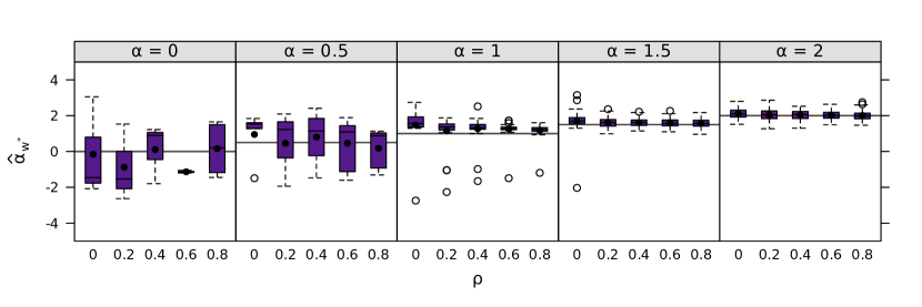
Figure 9: Simulation study: the selected $\rho^{*}$ according to the parameters $\rho$ and $\alpha$ (panel (a)) and $\hat{\alpha}$ obtained with INLA when we select $\mathcal{H}_{1}$ according to the Bayes Factor criterion (panel (b)) with a threshold of 100. The main horizontal lines correspond to the true value of the parameters $\rho$ and $\alpha$ in panels (a) and (b) respectively and the black points represent the mean estimates obtained.

C.3 Type I error in presence of censoring

Figure 10 shows that the type I error increases when the proportion of censoring increases.

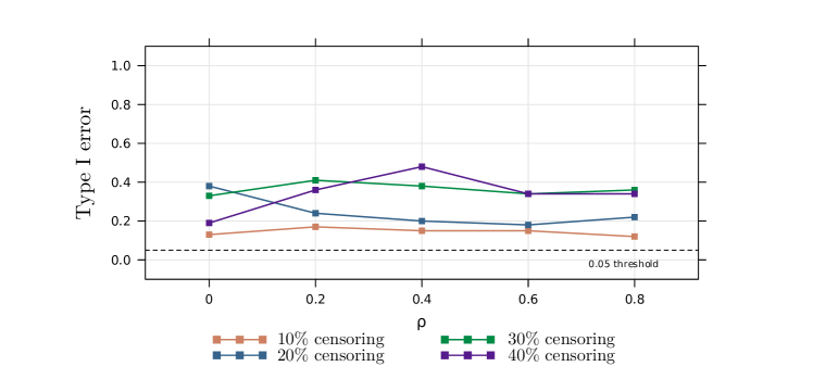
Figure 10: Simulation study: Comparison of the type I errors in the presence of censoring. $\rho$ controls the spatial correlation.

Appendix D Supplementary Materials of the application

Table LABEL:tab:confounders describes the confounding factors for the detection of clusters of abnormal survival times after starting dialysis in people aged 70 and over in the Nord-Pas-de-Calais region.

Table 2: Description of the confounding factors for the detection of clusters of abnormal survival times in ESRD elderly patients in northern France, 2004-2020.

Variable	Overall, $N=6071^{1}$
Age (in years)	79.0 (74.8;83.5)
Body mass index (in $\text{kg/m}^{2}$)	26.2 (23.0;30.1)
Sex (Woman)	2582/6071 (42.5%)
Type of nephropathy
Polycystic kidney disease	104/5342 (1.9%)
Primitive glomerulonephritis	427/5342 (8.0%)
Hypertension or vascular	2048/5342 (38.3%)
Diabetic nephropathy	1683/5342 (31.5%)
Pyelonephritis	283/5342 (5.3%)
Other	797/5342 (14.9%)
Number of cardiovascular comorbidities
None	962/5380 (17.9%)
One	1566/5380 (29.1%)
At least two	2852/5380 (53.0%)
Diabete (Yes)	3059/5960 (51.3%)
Chronic respiratory disease (Yes)	1062/5793 (18.3%)
Respiratory assistance (Yes)	380/5770 (6.6%)
Cirrhosis (Yes)	148/5804 (2.5%)
Severe behavioral disorder (Yes)	257/5532 (4.6%)
Mobility
Autonomous walking	3262/4930 (66.2%)
Need for a third party	1205/4930 (24.4%)
Total disability	463/4930 (9.4%)
Hemoglobin level ($<11\text{g/dL}$)	3760/5479 (68.6%)
Albumin level ($<35\text{g/dL}$)	2525/4786 (52.8%)
Dialysis method
Haemodialysis	5330/6071 (87.8%)
Peritoneal dialysis	741/6071 (12.2%)
Emergency start (Yes)	1776/5470 (32.5%)
Active malignancy (Yes)	586/5819 (10.1%)
Glomerular filtration rate
$<7\text{mL/min/1.73m}^{2}$	882/5285 (16.7%)
$7-10\text{mL/min/1.73m}^{2}$	1535/5285 (29.0%)
$>10\text{mL/min/1.73m}^{2}$	2868/5285 (54.3%)
Year of treatment initiation
2004-2009	1928/6071 (31.8%)
2010-2015	2258/6071 (37.2%)
2016-2020	1885/6071 (31.0%)

Figure 11 shows the posterior distributions of the frailty variance $\sigma^{2}$ with a i.i.d., a CAR and a ICAR model as well as the posterior distribution of the spatial correlation parameter $\rho$ of the frailty CAR model.

(a)

(b)

(c)

(d)

Figure 11: Posterior distribution of the frailty variance with the i.i.d. (panel (a)), CAR (panel (b)) and ICAR (panel (c)) models and posterior distribution of the spatial correlation parameter $\rho$ obtained with the CAR model (panel (d))

Figure 12 presents the estimated $\varphi_{k}$ for each model: the i.i.d. model, the Leroux CAR model and the ICAR model.

(a)

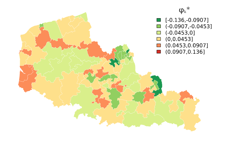
(b)

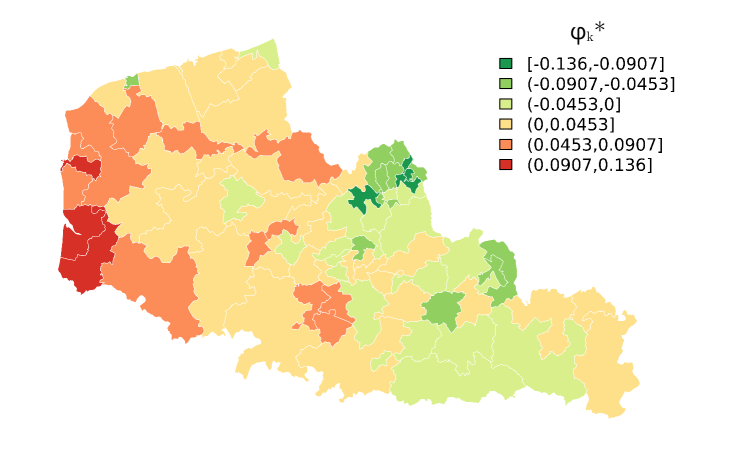
(c)

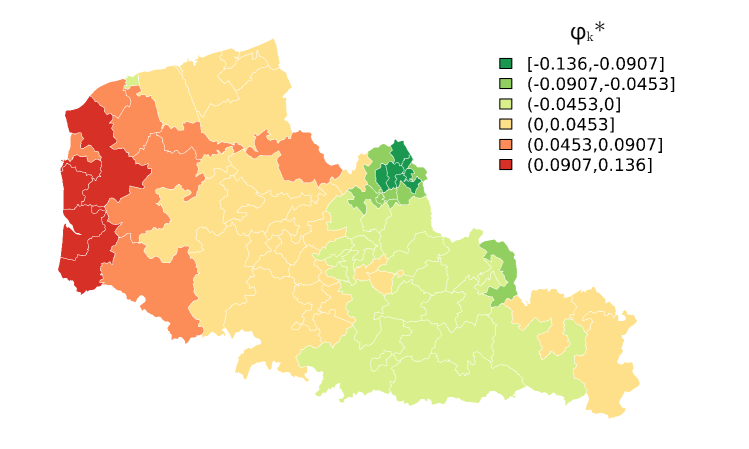
Figure 12: Estimated frailties $\varphi_{k}^{*}$ with the i.i.d. (panel (a)), CAR (panel (b)) and ICAR (panel (c)) models

References

- Abolhassani and Prates (2021) Abolhassani, A. and M. O. Prates (2021). An up-to-date review of scan statistics. Statistics Surveys 15, 111–153.
- Ahmed et al. (2021) Ahmed, M.-S., L. Cucala, and M. Genin (2021). Spatial autoregressive models for scan statistic. Journal of Spatial Econometrics 2(1), 1–20.
- Ahmed and Genin (2020) Ahmed, M.-S. and M. Genin (2020). A functional-model-adjusted spatial scan statistic. Statistics in Medicine 39(8), 1025–1040.
- Arlinghaus (1995) Arlinghaus, S. (1995). Practical handbook of spatial statistics. CRC press.
- Aswi et al. (2020) Aswi, A., S. Cramb, E. Duncan, W. Hu, G. White, and K. Mengersen (2020). Bayesian spatial survival models for hospitalisation of dengue: A case study of wahidin hospital in makassar, indonesia. International journal of environmental research and public health 17(3), 878.
- Austin (2017) Austin, P. C. (2017). A tutorial on multilevel survival analysis: methods, models and applications. International Statistical Review 85(2), 185–203.
- Ayav et al. (2016) Ayav, C., J.-B. Beuscart, S. Briançon, A. Duhamel, L. Frimat, and M. Kessler (2016). Competing risk of death and end-stage renal disease in incident chronic kidney disease (stages 3 to 5): the epiran community-based study. BMC nephrology 17(1), 1–13.
- Banerjee et al. (2003) Banerjee, S., M. M. Wall, and B. P. Carlin (2003). Frailty modeling for spatially correlated survival data, with application to infant mortality in minnesota. Biostatistics 4(1), 123–142.
- Besag (1974) Besag, J. (1974). Spatial interaction and the statistical analysis of lattice systems. Journal of the Royal Statistical Society. Series B (Methodological) 36(2), 192–236.
- Besag et al. (1991) Besag, J., J. York, and A. Mollié (1991). Bayesian image restoration, with two applications in spatial statistics. Annals of the institute of statistical mathematics 43(1), 1–20.
- Bhatt and Tiwari (2014) Bhatt, V. and N. Tiwari (2014). A spatial scan statistic for survival data based on weibull distribution. Statistics in medicine 33(11), 1867–1876.
- Brook (1964) Brook, D. (1964). On the distinction between the conditional probability and the joint probability approaches in the specification of nearest-neighbour systems. Biometrika 51, 481–483.
- Cançado et al. (2014) Cançado, A. L., C. Q. da Silva, and M. F. da Silva (2014). A spatial scan statistic for zero-inflated poisson process. Environmental and ecological statistics 21(4), 627–650.
- Cançado et al. (2017) Cançado, A. L., L. B. Fernandes, and C. Q. da Silva (2017). A bayesian spatial scan statistic for zero-inflated count data. Spatial Statistics 20, 57–75.
- Chen and Glaz (2009) Chen, J. and J. Glaz (2009). Approximations for two-dimensional variable window scan statistics. In J. Glaz, V. Pozdnyakov, and S. Wallenstein (Eds.), Scan Statistics, pp. 109 – 128. Birkhäuser Boston.
- Clayton (1978) Clayton, D. G. (1978). A model for association in bivariate life tables and its application in epidemiological studies of familial tendency in chronic disease incidence. Biometrika 65(1), 141–151.
- Cook et al. (2007) Cook, A. J., D. R. Gold, and Y. Li (2007). Spatial cluster detection for censored outcome data. Biometrics 63(2), 540–549.
- Couchoud et al. (2005) Couchoud, C., B. Stengel, P. Landais, J.-C. Aldigier, F. de Cornelissen, C. Dabot, H. Maheut, V. Joyeux, M. Kessler, M. Labeeuw, H. Isnard, and C. Jacquelinet (2005, 10). The renal epidemiology and information network (REIN): a new registry for end-stage renal disease in France. Nephrology Dialysis Transplantation 21(2), 411–418.
- Couchoud et al. (2015) Couchoud, C. G., J.-B. R. Beuscart, J.-C. Aldigier, P. J. Brunet, and O. P. Moranne (2015). Development of a risk stratification algorithm to improve patient-centered care and decision making for incident elderly patients with end-stage renal disease. Kidney international 88(5), 1178–1186.
- Crawford (2009) Crawford, T. (2009). Scale analytical. In R. Kitchin and N. Thrift (Eds.), International Encyclopedia of Human Geography, pp. 29–36. Oxford: Elsevier.
- Cressie (1977) Cressie, N. (1977). On some properties of the scan statistic on the circle and the line. Journal of Applied Probability 14, 272–283.
- Cucala et al. (2017) Cucala, L., M. Genin, C. Lanier, and F. Occelli (2017). A multivariate gaussian scan statistic for spatial data. Spatial Statistics 21.
- De La Fuente Marcos and De La Fuente Marcos (2008) De La Fuente Marcos, R. and C. De La Fuente Marcos (2008). From star complexes to the field: open cluster families. The Astrophysical Journal 672(1), 342.
- de Lima et al. (2015) de Lima, M. S., L. H. Duczmal, J. C. Neto, and L. P. Pinto (2015). Spatial scan statistics for models with overdispersion and inflated zeros. Statistica Sinica, 225–241.
- Dwass (1957) Dwass, M. (1957). Modified randomization tests for nonparametric hypotheses. Annals of Mathematical Statistics 28(1), 181–187.
- Fine and Gray (1999) Fine, J. P. and R. J. Gray (1999). A proportional hazards model for the subdistribution of a competing risk. Journal of the American statistical association 94(446), 496–509.
- Frévent et al. (2021) Frévent, C., M.-S. Ahmed, M. Marbac, and M. Genin (2021, 12). Detecting spatial clusters in functional data: new scan statistic approaches. Spatial Statistics 46, 100550.
- Frévent et al. (2021) Frévent, C., M.-S. Ahmed, S. Dabo-Niang, and M. Genin (2021, 03). Investigating spatial scan statistics for multivariate functional data. arXiv preprint arXiv:2103.14401.
- Fu et al. (2021) Fu, E. L., M. Evans, J.-J. Carrero, H. Putter, C. M. Clase, F. J. Caskey, M. Szymczak, C. Torino, N. C. Chesnaye, K. J. Jager, et al. (2021). Timing of dialysis initiation to reduce mortality and cardiovascular events in advanced chronic kidney disease: nationwide cohort study. bmj 375.
- Genin et al. (2020) Genin, M., M. Fumery, F. Occelli, G. Savoye, B. Pariente, L. Dauchet, J. Giovannelli, C. Vignal, M. Body-Malapel, H. Sarter, et al. (2020). Fine-scale geographical distribution and ecological risk factors for crohn’s disease in france (2007-2014). Alimentary Pharmacology & Therapeutics 51(1), 139–148.
- Green et al. (2006) Green, C., L. Elliott, C. Beaudoin, and C. N. Bernstein (2006). A population-based ecologic study of inflammatory bowel disease: searching for etiologic clues. American journal of epidemiology 164(7), 615–623.
- Gregorio et al. (2007) Gregorio, D. I., L. Huang, L. M. DeChello, H. Samociuk, and M. Kulldorff (2007). Place of residence effect on likelihood of surviving prostate cancer. Annals of epidemiology 17(7), 520–524.
- Hallan et al. (2012) Hallan, S. I., K. Matsushita, Y. Sang, B. K. Mahmoodi, C. Black, A. Ishani, N. Kleefstra, D. Naimark, P. Roderick, M. Tonelli, J. F. M. Wetzels, B. C. Astor, R. T. Gansevoort, A. Levin, C.-P. Wen, J. Coresh, and f. t. Chronic Kidney Disease Prognosis Consortium (2012, 12). Age and Association of Kidney Measures With Mortality and End-stage Renal Disease. JAMA 308(22), 2349–2360.
- Henry et al. (2009) Henry, K. A., X. Niu, and F. P. Boscoe (2009). Geographic disparities in colorectal cancer survival. International journal of health geographics 8(1), 1–13.
- Hougaard (2000) Hougaard, P. (2000). Shared frailty models, pp. 215–262. New York, NY: Springer New York.
- Huang et al. (2007) Huang, L., M. Kulldorff, and D. Gregorio (2007). A spatial scan statistic for survival data. Biometrics 63(1), 109–118.
- Jeffreys (1961) Jeffreys, H. (1961). Theory of probability (3rd Ed.). Oxford, UK: Oxford University Press.
- Jung (2009) Jung, I. (2009). A generalized linear models approach to spatial scan statistics for covariate adjustment. Statistics in medicine 28(7), 1131–1143.
- Jung et al. (2007) Jung, I., M. Kulldorff, and A. C. Klassen (2007). A spatial scan statistic for ordinal data. Statistics in medicine 26(7), 1594–1607.
- Khan et al. (2021) Khan, M. M., S. Roberson, K. Reid, M. Jordan, and A. Odoi (2021). Geographic disparities and temporal changes of diabetes prevalence and diabetes self-management education program participation in florida. Plos one 16(7).
- Kleinbaum and Klein (2012) Kleinbaum, D. G. and M. Klein (2012). Recurrent event survival analysis. In Survival Analysis, pp. 363–423. Springer.
- Kulldorff (1997) Kulldorff, M. (1997). A spatial scan statistic. Communications in Statistics - Theory and Methods 26, 1481–1496.
- Kulldorff et al. (2009) Kulldorff, M., L. Huang, and K. Konty (2009). A scan statistic for continuous data based on the normal probability model. Int J Health Geogr 8(58).
- Kulldorff et al. (2006) Kulldorff, M., L. Huang, L. Pickle, and L. Duczmal (2006). An elliptic spatial scan statistic. Statistics in medicine 25, 3929–3943.
- Kulldorff et al. (2007) Kulldorff, M., F. Mostashari, L. Duczmal, W. Katherine Yih, K. Kleinman, and R. Platt (2007). Multivariate scan statistics for disease surveillance. Statistics in medicine 26(8), 1824–1833.
- Kulldorff and Nagarwalla (1995) Kulldorff, M. and N. Nagarwalla (1995). Spatial disease clusters: Detection and inference. Statistics in Medicine 14(8), 799–810.
- Lee et al. (2020) Lee, J., Y. Sun, and H. H. Chang (2020). Spatial cluster detection of regression coefficients in a mixed-effects model. Environmetrics 31(2), e2578.
- Leiser et al. (2020) Leiser, C. L., M. Taddie, R. Hemmert, R. Richards Steed, J. A. VanDerslice, K. Henry, J. Ambrose, B. O’Neil, K. R. Smith, and H. A. Hanson (2020). Spatial clusters of cancer incidence: Analyzing 1940 census data linked to 1966–2017 cancer records. Cancer Causes & Control 31(7), 609–615.
- Leroux et al. (2000) Leroux, B. G., X. Lei, and N. Breslow (2000). Estimation of disease rates in small areas: a new mixed model for spatial dependence. In Statistical models in epidemiology, the environment, and clinical trials, pp. 179–191. Springer.
- Li (2009) Li, Y. (2009). Modeling and analysis of spatially correlated data. New Developments In Biostatistics And Bioinformatics, 72–98.
- Li and Ryan (2002) Li, Y. and L. Ryan (2002). Modeling spatial survival data using semiparametric frailty models. Biometrics 58(2), 287–297.
- Liang et al. (1995) Liang, K.-Y., S. G. Self, K. J. Bandeen-Roche, and S. L. Zeger (1995). Some recent developments for regression analysis of multivariate failure time data. Lifetime data analysis 1(4), 403–415.
- Lin (2014) Lin, P.-S. (2014). Generalized scan statistics for disease surveillance. Scandinavian Journal of Statistics 41(3), 791–808.
- Loh and Zhu (2007) Loh, J. M. and Z. Zhu (2007). Accounting for spatial correlation in the scan statistic. The Annals of Applied Statistics 1(2), 560–584.
- Marciano et al. (2018) Marciano, L. H. S. C., A. de Faria Fernandes Belone, P. S. Rosa, N. M. B. Coelho, C. C. Ghidella, S. M. T. Nardi, W. C. Miranda, L. V. Barrozo, and J. C. Lastória (2018). Epidemiological and geographical characterization of leprosy in a brazilian hyperendemic municipality. Cadernos de saude publica 34.
- Minamisava et al. (2009) Minamisava, R., S. S. Nouer, O. L. de Morais Neto, L. K. Melo, and A. L. S. Andrade (2009). Spatial clusters of violent deaths in a newly urbanized region of brazil: highlighting the social disparities. International journal of health geographics 8(1), 1–10.
- Montez-Rath et al. (2017) Montez-Rath, M. E., K. Kapphahn, M. B. Mathur, A. A. Mitani, D. J. Hendry, and M. Desai (2017). Guidelines for generating right-censored outcomes from a cox model extended to accommodate time-varying covariates. Journal of Modern Applied Statistical Methods 16(1), 6.
- Neill and Cooper (2010) Neill, D. B. and G. F. Cooper (2010). A multivariate bayesian scan statistic for early event detection and characterization. Machine learning 79(3), 261–282.
- Ojiambo and Kang (2013) Ojiambo, P. and E. Kang (2013). Modeling spatial frailties in survival analysis of cucurbit downy mildew epidemics. Phytopathology 103(3), 216–227.
- Rondeau (2010) Rondeau, V. (2010). Statistical models for recurrent events and death: Application to cancer events. Mathematical and Computer modelling 52(7-8), 949–955.
- Rue et al. (2009) Rue, H., S. Martino, and N. Chopin (2009). Approximate bayesian inference for latent gaussian models by using integrated nested laplace approximations. Journal of the royal statistical society: Series b (statistical methodology) 71(2), 319–392.
- Shi et al. (2021) Shi, G., J. Liu, and X. Zhong (2021). Spatial and temporal variations of pm2.5 concentrations in chinese cities during 2015-2019. International Journal of Environmental Health Research, 1–13.
- Smida et al. (2022) Smida, Z., L. Cucala, A. Gannoun, and G. Durif (2022). A wilcoxon-mann-whitney spatial scan statistic for functional data. Computational Statistics & Data Analysis 167, 107378.
- Tango and Takahashi (2005) Tango, T. and K. Takahashi (2005). A flexibly shaped spatial scan statistic for detecting clusters. International journal of health geographics 4(1), 1–15.
- Usman and Rosychuk (2018) Usman, I. and R. J. Rosychuk (2018). A log-weibull spatial scan statistic for time to event data. International Journal of Health Geographics 17(1), 1–12.
- Wan et al. (2020) Wan, L., Y. Sun, I. Lee, W. Zhao, and F. Xia (2020). Industrial pollution areas detection and location via satellite-based iiot. IEEE Transactions on Industrial Informatics 17(3), 1785–1794.
- Wan et al. (2012) Wan, N., F. B. Zhan, Y. Lu, and J. P. Tiefenbacher (2012). Access to healthcare and disparities in colorectal cancer survival in texas. Health & place 18(2), 321–329.
- Yin and Mu (2018) Yin, P. and L. Mu (2018). A hybrid method for fast detection of spatial disease clusters in irregular shapes. GeoJournal 83(4), 693–705.
- Zhang et al. (2012) Zhang, T., Z. Zhang, and G. Lin (2012). Spatial scan statistics with overdispersion. Statistics in medicine 31(8), 762–774.
- Zhou et al. (2015) Zhou, R., L. Shu, and Y. Su (2015). An adaptive minimum spanning tree test for detecting irregularly-shaped spatial clusters. Computational Statistics & Data Analysis 89, 134–146.