$B$-anomalies in a twin Pati-Salam theory of flavour including the 2022 LHCb $R_{K^{(*)}}$ analysis

Abstract

We perform a comprehensive phenomenological analysis of the twin Pati-Salam theory of flavour, focussing on the parameter space relevant for interpreting the $B$-anomalies via vector leptoquark $U_{1}$ exchange. This model provides a very predictive framework in which the $U_{1}$ couplings and the Yukawa couplings find a common origin via mixing of chiral quarks and leptons with vector-like fermions, providing a direct link between the $B$-anomalies and the fermion masses and mixing. We propose and study a simplified model with three vector-like fermion families, in the massless first family approximation, and show that the second and third family charged fermion masses and mixings and the $B$-anomalies can be simultaneously explained and related. The model has the proper flavour structure to be compatible with all low-energy observables, and leads to predictions in promising observables such as $\tau\rightarrow 3\mu$, $\tau\rightarrow\mu\gamma$ and $B\rightarrow K^{(*)}\nu\bar{\nu}$ at Belle II and LHCb. The model also predicts a rich spectrum of TeV scale gauge bosons and vector-like fermions, all accessible to the LHC. In this updated version we have included an extended analysis considering the new 2022 LHCb data on $R_{K^{(*)}}$, which has slightly shifted the preferred parameter space with respect to the 2021 case. The model can still explain the $R_{D^{(*)}}$ anomalies at 1$\sigma$ in a narrow window, however we expect small deviations from the SM on the $R_{K^{(*)}}$ ratios, to be tested in the future via more precise measurements by the LHCb collaboration. We also predict $\Delta R_{D}=\Delta R_{D^{*}}$, with future measurements shifting the world averages to slightly smaller central values.

1 Introduction

Fundamental fermions in the Standard Model (SM) come in three copies, denoted as “flavours”, which share universal gauge interactions but have different masses and mixings, also known as flavour parameters. The origin of flavour in the SM remains as a complete mystery, as it lacks of any dynamical explanation to the high number of flavour parameters and their hierarchical patterns. A further theory of flavour beyond the SM should provide a solution to the long-lasting “flavour puzzle”.

Simultaneously, the non-universal structure of such a theory of flavour could leave its imprints in flavour physics observables, which are becoming accessible up to a high precision level in the current generation of colliders and meson factories. Given the prolific history of flavour physics anticipating the discovery of new physics, searching for the origin of flavour in flavour physics is well motivated. In this direction, a conspicuous series of anomalies in flavour observables emerged in the last years.

Back in 2021, when this project was started, the $R_{K^{(*)}}$ ratios had been measured by LHCb to be smaller than 1 LHCb:2017avl ; LHCb:2021trn , in good agreement with other anomalies in $b\rightarrow s\mu\mu$ data which were hinting for flavourful new physics (NP) affecting muons rather than electrons. In particular, $R_{K}^{[1.1,6]}$ was alone in more than 3$\sigma$ tension with the SM prediction. The breaking of SM lepton flavour universality (LFU) was not only suggested by $R_{K^{(*)}}$, but also the ratios $R_{D^{(*)}}$ had been measured to show discrepancy with the SM (see the world averages in HFLAV:2022pwe ), hinting for flavourful NP affecting tau leptons. Although no single measurement of $R_{D^{(*)}}$ is very significant, the combination of all of them hints for a consistent deviation from the SM prediction with more than 3$\sigma$ significance. Both LFU ratios together gave rise to a very consistent picture of hierarchical anomalies, where strong NP mainly coupled to the third family interfere with a SM charged current tree-level effect, while weaker NP couple to the much lighter muons, interfering with 1-loop and GIM-suppressed SM neutral currents.

This picture of “$B$-anomalies” led to important model building efforts by the community during the last 8 years, in order to interpret these anomalies as a low energy signal of a consistent NP model. A massive, electrically neutral $Z^{\prime}$ vector was identified as a possible explanation of the $R_{K^{(*)}}$ anomalies (see e.g. Crivellin:2015mga ; Crivellin:2015lwa ; Chiang:2017hlj ; King:2017anf ; Falkowski:2018dsl ; Navarro:2021sfb ), while different leptoquarks were proposed to address either $R_{K^{(*)}}$ or $R_{D^{(*)}}$ separately (see e.g. Becirevic:2017jtw ; deMedeirosVarzielas:2018bcy ; Angelescu:2021lln ; Becirevic:2022tsj ). Interestingly, the vector leptoquark $U_{1}(\boldsymbol{3},\boldsymbol{1},2/3)$ was identified as the only single mediator capable of addressing both $B$-anomalies simultaneously Angelescu:2021lln . However, the gauge nature of $U_{1}$ requires to specify a clear ultra-violet (UV) completion that explains its origin. The original ideas by Pati and Salam (PS) Pati:1974yy , led to tensions with unobserved processes such as $K_{L}\rightarrow\mu e$. Instead, an interesting proposal was firstly laid out in the Appendix of Diaz:2017lit , and more formally later in DiLuzio:2017vat , following the idea introduced in Georgi:2016xhm that color could appear as a diagonal subgroup of a larger $SU(3+N)\times SU(3)^{\prime}$ local symmetry valid at high energies. The particular choice $N=1$ leads to the so-called “4321” gauge symmetry,

$$G_{4321}\equiv SU(4)\times SU(3)_{c}^{{}^{\prime}}\times SU(2)_{L}\times U(1)_{Y^{\prime}}\,,$$ (1.1)

which can be broken at the TeV scale while satisfying the experimental bounds DiLuzio:2017vat ; DiLuzio:2018zxy ; Cornella:2019hct ; Cornella:2021sby , provided that at least the first and second families of SM fermions are singlets under $SU(4)$. This breaking leads to a rich gauge boson spectrum at the TeV scale, containing the vector leptoquark $U_{1}$ along with a massive colour octet $g^{\prime}(\boldsymbol{8},\boldsymbol{1},0)$ and a massive $Z^{\prime}\left(\boldsymbol{1},\boldsymbol{1},0\right)$ with suppressed couplings to light SM fermions. Vector-like (VL) fermions need to be introduced in order to obtain effective couplings of (at least) second family fermions to $U_{1}$. The model, even if not minimal, is very predictive and leads to a rich phenomenology in both low-energy and high-$p_{T}$ searches. However, the flavour structure of the model was rather ad-hoc, and it was hinted that the 4321 gauge group could be the TeV scale effective field theory of a complete model addressing more open questions of the SM. In particular, the 4321 model seemed to be a nice playground to connect the picture of $B$-anomalies with the flavour puzzle of the SM.

Motivated by the desire to link the origin of the $B$-anomalies with the origin of Yukawa couplings in the SM, one of us proposed a theory of flavour involving a twin Pati-Salam group King:2021jeo . Unlike the other models already present in the market Bordone:2017bld ; Bordone:2018nbg ; Fuentes-Martin:2022xnb , the twin PS treats all three fermion families in the same way. The basic idea is that all three families of SM chiral fermions transform under one PS group, while families of vector-like fermions transform under the other one. The first PS group, broken at a high scale, provides Pati-Salam unification of all SM quarks and leptons, while a fourth family of vector-like fermions transforms under a second PS group, broken at the TeV scale to the SM, as in Fig. 1.1. The full twin Pati-Salam symmetry, together with the absence of a standard Higgs electroweak (EW) doublet, forbids the usual Yukawa couplings for the SM fermions. Instead, effective Yukawa couplings arise through the mixing between SM fermions and vector-like partners. The same mixing leads to $U_{1}$ couplings for SM fermions which could address the $B$-anomalies. This way, $B$-anomalies and the flavour puzzle are dynamically and parametrically connected. Furthermore, the twin PS model predicts dominantly left-handed (LH) $U_{1}$ currents that were preferred by the 2021 picture of $B$-anomalies Geng:2021nhg ; Angelescu:2021lln ; Altmannshofer:2021qrr , while the other proposals Bordone:2017bld ; Bordone:2018nbg ; Fuentes-Martin:2022xnb predict large couplings for right-handed (RH) third family fermion, which lead to tight constraints from high-$p_{T}$ searches.

In this paper, we studied the phenomenology of the simplified twin PS model presented in King:2021jeo , which turned out to be incompatible with low-energy data. Afterwards, we performed further model building and presented an extended version of the model that can explain the 2021 picture of $B$-anomalies and address charged fermion masses and mixings, while being compatible with all existing data. However, during the peer-review process of this paper, the LHCb collaboration presented a reanalysis of the LFU ratios $R_{K^{(*)}}$, with the new measurements in the central $q^{2}$ shown below (where $q^{2}$ denotes the dilepton invariant-mass squared) LHCb:2022qnv

$$R_{K}^{[1.1,6]}=\frac{\mathrm{Br}\left(B\rightarrow K\mu^{+}\mu^{-}\right)}{\mathrm{Br}\left(B\rightarrow Ke^{+}e^{-}\right)}=0.949_{-0.046}^{+0.047}\,,\qquad R_{K^{*}}^{[1.1,6]}=\frac{\mathrm{Br}\left(B\rightarrow K^{*}\mu^{+}\mu^{-}\right)}{\mathrm{Br}\left(B\rightarrow K^{*}e^{+}e^{-}\right)}=1.027_{-0.073}^{+0.077}\,,$$ (1.2)

with correlation $\rho=-0.017$. Unexpectedly, the updated results are in good agreement with the SM predictions of $R_{K^{(*)}}^{[1.1,6]}=1\pm 0.01$ Bordone:2016gaq , as a result of backgrounds in the electron channel which were misidentified in all the previous analyses. Although our model was originally built to explain large deviations from the SM in both $R_{K^{(*)}}$ and $R_{D^{(*)}}$, the new experimental data offers the opportunity to further test the model as a legitimate theory of flavour addressing the origin of quark and lepton masses and mixings. Therefore, we present here an updated analysis which includes the new 2022 LHCb data on $R_{K^{(*)}}$, and we confront the new results versus the previous 2021 picture for which the model was intended. Beyond the $R_{K^{(*)}}$ ratios, a new combined measurement of $R_{D^{(*)}}$ was presented by LHCb in late 2022 LHCb:2023zxo . This measurement is in line with the previous experimental data on $R_{D^{(*)}}$, and does not significantly modify the HFLAV average HFLAV:2022pwe ,

$$R_{D}=\left.\frac{\mathrm{Br}\left(B\rightarrow D\tau\nu\right)}{\mathrm{Br}\left(B\rightarrow D\ell\nu\right)}\right|_{\ell\epsilon\,\left\{e,\mu\right\}}=0.358\pm 0.028\,,\qquad R_{D^{*}}=\left.\frac{\mathrm{Br}\left(B\rightarrow D^{*}\tau\nu\right)}{\mathrm{Br}\left(B\rightarrow D^{*}\ell\nu\right)}\right|_{\ell\epsilon\,\left\{e,\mu\right\}}=0.285\pm 0.013\,.$$ (1.3)

which remains at roughly 3$\sigma$ discrepancy with the SM predictions.

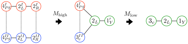
Figure 1.1: The model is based on two copies of the Pati-Salam gauge group $SU(4)_{PS}\times SU(2)_{L}\times SU(2)_{R}$. The circles represent the gauge groups with the indicated symmetry breaking. The twin Pati-Salam symmetry is broken down to the 4321 symmetry at high energies $M_{\mathrm{High}}\apprge 1\,\mathrm{PeV}$, then the 4321 group is further broken to the SM at the TeV scale $M_{\mathrm{low}}\sim\mathcal{O}(\mathrm{TeV}).$

The layout of the remainder of the paper is as follows. In Section 2 we introduce the simplified twin Pati-Salam model as presented in King:2022sxb , featuring only one vector-like family, and show that it is unable to explain $R_{D^{(*)}}$ in a natural way, while being compatible with the stringent constraints from $B_{s}-\bar{B}_{s}$ mixing. Instead, in Section 3 we present a new, extended version of the twin Pati-Salam model including three vector-like families and a discrete flavour symmetry, which is compatible with low-energy data and high-$p_{T}$ searches. Section 3.2 shows how effective Yukawa couplings for the SM fermions arise in the model, addressing charged fermions masses and mixings. Similarly, Section 3.3 shows the origin of effective couplings between SM fermions and the exotic gauge bosons. Section 3.4 shows the phenomenological analysis and the discussion of the results, including promising signals to test the model in low-energy observables and high-$p_{T}$ searches, along with a study of the perturbativity of the model. Section 4 includes a comparison of our predictions with other models in the market. Finally, we conclude the paper in Section 5.

2 Simplified twin Pati-Salam theory of flavour

2.1 The High Energy Model

In the traditional PS theory, the chiral quarks and leptons are unified into $SU(4)_{PS}$ multiplets with leptons as the fourth colour (red, blue, green, lepton) Pati:1974yy ,

$$\psi_{i}(4,2,1)=\left(\begin{array}[]{cccc}u_{r}&u_{b}&u_{g}&\nu\\ d_{r}&d_{b}&d_{g}&e\end{array}\right)_{i}\equiv\left(Q_{i},L_{i}\right)\,,\quad\psi_{j}^{c}(\overline{4},1,\overline{2})=\left(\begin{array}[]{cccc}u_{r}^{c}&u_{b}^{c}&u_{g}^{c}&\nu^{c}\\ d_{r}^{c}&d_{b}^{c}&d_{g}^{c}&e^{c}\end{array}\right)_{j}\equiv\left(u_{j}^{c},d_{j}^{c},\nu_{j}^{c},e_{j}^{c}\right)\,,$$ (2.1)

where $\psi_{i}$ contains the left-handed quark and leptons while $\psi_{j}^{c}$ contains the CP-conjugated right-handed (RH) quarks and lepton (so that they become LH), and $i,j=1,2,3$ are family indices. We consider here two copies of the Pati-Salam symmetry King:2021jeo ,

$$G_{422}^{I}\times G_{422}^{II}=\left(SU(4)_{PS}^{I}\times SU(2)_{L}^{I}\times SU(2)_{R}^{I}\right)\times\left(SU(4)_{PS}^{II}\times SU(2)_{L}^{II}\times SU(2)_{R}^{II}\right)\,.$$ (2.2)

The matter content and the quantum numbers of each field are displayed in Table 1. The usual three chiral fermion families, SM-like, originate from the second PS group $G_{422}^{II}$, broken at a high scale, and transform under Eq. (2.2) as

$$\psi_{1,2,3}(1,1,1;4,2,1)\,,\quad\psi_{1,2,3}^{c}(1,1,1;\overline{4},1,\overline{2})\,.$$ (2.3)

This simplified version of the theory includes one vector-like family of fermions which originates under the first PS group, whose $SU(4)^{I}$ is broken at the TeV scale, and transforms under Eq. (2.2) as

$$\psi_{4}(4,2,1;1,1,1)\,,\quad\overline{\psi_{4}}(\overline{4},\overline{2},1;1,1,1)\,,\psi_{4}^{c}(\overline{4},1,\overline{2};1,1,1)\,,\overline{\psi_{4}^{c}}(4,1,2;1,1,1)\,.$$ (2.4)

On the other hand, according to the matter content in Table 1, there are no standard Higgs fields which transform as ($1,\overline{2},2$) under $G_{422}^{II}$, hence the standard Yukawa couplings involving the chiral fermions are forbidden by the twin PS symmetry. These will be generated effectively via mixing with the fourth family of vector-like fermions which only have quantum numbers under the first PS group, $G_{422}^{I}$. This mixing is facilitated by the non-standard Higgs scalar doublets contained in $\phi$, $\overline{\phi}$, $H$, $\overline{H}$ in Table 1, via the couplings,

Field	$SU(4)_{PS}^{I}$	$SU(2)_{L}^{I}$	$SU(2)_{R}^{I}$	$SU(4)_{PS}^{II}$	$SU(2)_{L}^{II}$	$SU(2)_{R}^{II}$
$\psi_{1,2,3}$	$\mathbf{1}$	$\mathbf{1}$	$\mathbf{1}$	$\mathbf{4}$	$\mathbf{2}$	$\mathbf{1}$
$\psi_{1,2,3}^{c}$	$\mathbf{1}$	$\mathbf{1}$	$\mathbf{1}$	$\mathbf{\overline{4}}$	$\mathbf{1}$	$\mathbf{\overline{2}}$
$\psi_{4}$	$\mathbf{4}$	$\mathbf{2}$	$\mathbf{1}$	$\mathbf{1}$	$\mathbf{1}$	$\mathbf{1}$
$\overline{\psi_{4}}$	$\mathbf{\overline{4}}$	$\mathbf{\overline{2}}$	$\mathbf{1}$	$\mathbf{1}$	$\mathbf{1}$	$\mathbf{1}$
$\psi_{4}^{c}$	$\mathbf{\overline{4}}$	$\mathbf{1}$	$\mathbf{\overline{2}}$	$\mathbf{1}$	$\mathbf{1}$	$\mathbf{1}$
$\overline{\psi_{4}^{c}}$	$\mathbf{4}$	$\mathbf{1}$	$\mathbf{2}$	$\mathbf{1}$	$\mathbf{1}$	$\mathbf{1}$
$\phi$	$\mathbf{4}$	$\mathbf{2}$	$\mathbf{1}$	$\mathbf{\overline{4}}$	$\mathbf{\overline{2}}$	$\mathbf{1}$
$\overline{\phi}$	$\mathbf{\overline{4}}$	$\mathbf{1}$	$\mathbf{\overline{2}}$	$\mathbf{4}$	$\mathbf{1}$	$\mathbf{2}$
$H$	$\mathbf{\overline{4}}$	$\mathbf{\overline{2}}$	$\mathbf{1}$	$\mathbf{4}$	$\mathbf{1}$	$\mathbf{2}$
$\overline{H}$	$\mathbf{4}$	$\mathbf{1}$	$\mathbf{2}$	$\mathbf{\overline{4}}$	$\mathbf{\overline{2}}$	$\mathbf{1}$
$H^{\prime}$	$\mathbf{1}$	$\mathbf{1}$	$\mathbf{1}$	$\mathbf{4}$	$\mathbf{1}$	$\mathbf{2}$
$\Phi$	$\mathbf{1}$	$\mathbf{2}$	$\mathbf{1}$	$\mathbf{1}$	$\mathbf{\overline{2}}$	$\mathbf{1}$
$\overline{\Phi}$	$\mathbf{1}$	$\mathbf{1}$	$\mathbf{\overline{2}}$	$\mathbf{1}$	$\mathbf{1}$	$\mathbf{2}$

Table 1: The field content under $G_{422}^{I}\times G_{422}^{II}$, see the main text for details.

$$\mathcal{L}_{\mathrm{mass}}^{ren}=y_{i4}^{\psi}\overline{H}\psi_{i}\psi_{4}^{c}+y_{4i}^{\psi}H\psi_{4}\psi_{i}^{c}+x_{i4}^{\psi}\phi\psi_{i}\overline{\psi_{4}}+x_{4i}^{\psi^{c}}\overline{\psi_{4}^{c}\phi}\psi_{i}^{c}+M_{4}^{\psi}\psi_{4}\overline{\psi_{4}}+M_{4}^{\psi^{c}}\psi_{4}^{c}\overline{\psi_{4}^{c}}\,,$$ (2.5)

plus h.c., where $i=1,2,3$; $x,y$ are dimensionless universal coupling constants and $M_{4}^{\psi,\psi^{c}}$ are the VL mass terms. These couplings mix the chiral fermions with the VL fermions, and will be responsible for generating effective Yukawa couplings for the second and third families. Moreover, the same mixing leads to effective couplings to TeV scale $SU(4)^{I}$ gauge bosons which violate lepton universality between the second and third families, as we shall see.

2.2 High scale symmetry breaking

The twin Pati-Salam symmetry displayed in Eq. (2.2) is spontaneously broken to the “4321” symmetry at the high scale $M_{\mathrm{High}}\apprge 1\,\mathrm{PeV}$ (the latter bound due to the non-observation of $K_{L}\rightarrow\mu e$ Valencia:1994cj ),

$$G_{422}^{I}\times G_{422}^{II}\rightarrow G_{4321}\equiv SU(4)_{PS}^{I}\times SU(3)_{c}^{II}\times SU(2)_{L}^{I+II}\times U(1)_{Y^{\prime}}\,.$$ (2.6)

We can think of this as a two part symmetry breaking:
(i) The two pairs of left-right groups break down to their diagonal left-right subgroup, via the VEVs $\left\langle\Phi\right\rangle\sim v_{\Phi}$ and $\langle\overline{\Phi}\rangle\sim v_{\overline{\Phi}}$, leading to the symmetry breaking,

$$SU(2)_{L}^{I}\times SU(2)_{L}^{II}\rightarrow SU(2)_{L}^{I+II}\,,\qquad SU(2)_{R}^{I}\times SU(2)_{R}^{II}\rightarrow SU(2)_{R}^{I+II}\,.$$ (2.7)

Since the two $SU(4)_{PS}$ groups remain intact, the above symmetry breaking corresponds to

$$G_{422}^{I}\times G_{422}^{II}\rightarrow G_{4422}\equiv SU(4)_{PS}^{I}\times SU(4)_{PS}^{II}\times SU(2)_{L}^{I+II}\times SU(2)_{R}^{I+II}\,.$$ (2.8)

(ii) Then we assume the second PS group is broken at a high scale via the Higgs $H^{\prime}$ in Table 1, which under $G_{4422}$ transform as

$$H^{\prime}(1,4,1,2)=\left(\begin{array}[]{cccc}u_{H^{\prime}}^{r}&u_{H^{\prime}}^{b}&u_{H^{\prime}}^{g}&\nu_{H^{\prime}}\\ d_{H^{\prime}}^{r}&d_{H^{\prime}}^{b}&d_{H^{\prime}}^{g}&e_{H^{\prime}}\end{array}\right)\,,$$ (2.9)

and develops VEV in its right-handed neutrino component,$\left\langle\nu_{H^{\prime}}\right\rangle\apprge 1\,\mathrm{PeV}$, leading to the symmetry breaking

$$G_{4422}\rightarrow G_{4321}\equiv SU(4)_{PS}^{I}\times SU(3)_{c}^{II}\times SU(2)_{L}^{I+II}\times U(1)_{Y^{\prime}}\,,$$ (2.10)

where $SU(4)_{PS}^{II}$ is broken to $SU(3)_{c}^{II}\times U(1)_{B-L}^{II}$ (at the level of fermion representations, chiral quarks and leptons are split $\mathbf{4}^{II}\rightarrow(\mathbf{3},1/6)^{II}\oplus(\mathbf{1},-1/2)^{II}$), while $SU(2)_{R}^{I+II}$ is broken to $U(1)_{T_{3R}}^{I+II}$ and the abelian generators are broken to $U(1)_{Y^{\prime}}$, where $Y^{\prime}=T_{B-L}^{II}+T_{3R}^{I+II}$. The broken generators of $SU(4)_{PS}^{II}$ are associated with PeV-scale gauge bosons that will mediate processes at acceptable rates, beyond the sensitivity of current experiments and colliders. Instead, the further symmetry breaking of $G_{4321}$ will lead to a rich phenomenology at the TeV scale, as we shall see. We anticipate that $SU(2)_{L}^{I+II}$ is already the $SU(2)_{L}$ of the SM gauge group, while SM color and hypercharge are embedded in $SU(4)_{PS}^{I}\times SU(3)_{c}^{II}\times U(1)_{Y^{\prime}}$.

On the other hand, the Yukon scalars $\phi$ and $\overline{\phi}$ in Table 1 decompose under $G_{422}^{I}\times G_{422}^{II}\rightarrow G_{4422}\rightarrow G_{4321}$ as

$$\begin{array}[]{c}\phi(\mathbf{4,2,1;\overline{4},\overline{2},1})\rightarrow\phi(\mathbf{4,\overline{4},1\oplus 3,1})\rightarrow\phi_{3}(\mathbf{4,\overline{3},1\oplus 3},-1/6)\oplus\phi_{1}(\mathbf{4,1,1\oplus 3},1/2)\,,\\ \\ \overline{\phi}(\mathbf{\overline{4},1,\overline{2};4,1,2})\rightarrow\overline{\phi}(\mathbf{\overline{4},4,1,1\oplus 3})\rightarrow\overline{\phi_{3}}(\mathbf{\overline{4},3,1},1/6)\oplus\overline{\phi_{1}}(\mathbf{\overline{4},1,1},-1/2)\,,\end{array}$$ (2.11)

plus extra $\overline{\phi_{3}}$ and $\overline{\phi_{1}}$ with different values of $Y^{\prime}$ associated to the breaking of the $SU(2)_{R}^{I+II}$ triplet, that we ignore because they do not couple to fermions. The decomposition above is of phenomenological interest, as the Yukons $\phi_{3}$, $\overline{\phi_{3}}$ will couple to quarks while $\phi_{1}$, $\overline{\phi_{1}}$ will couple to leptons, allowing non-trivial mixing between SM fermions and VL fermions. They will also lead to a non-trivial breaking of $G_{4321}$ down to the SM.

The Higgs scalars $H$ and $\overline{H}$ in Table 1 decompose under $G_{422}^{I}\times G_{422}^{II}\rightarrow G_{4321}$ as (we skip the $G_{4422}$ decomposition here for simplicity)

$$H(\mathbf{\overline{4},\overline{2},1;4,1,2})\rightarrow H_{t}(\mathbf{\overline{4},3,\overline{2}},2/3),\>H_{b}(\mathbf{\overline{4},3,\overline{2}},-1/3),\,H_{\tau}(\mathbf{\overline{4},1,\overline{2}},-1),\,H_{\nu_{\tau}}(\mathbf{\overline{4},1,\overline{2}},0)\,,$$ (2.12)

$$\overline{H}(\mathbf{4,1,2;\overline{4},\overline{2},1})\rightarrow H_{c}(\mathbf{4,\overline{3},\overline{2}},1/3),\>H_{s}(\mathbf{4,\overline{3},\overline{2}},-2/3),\,H_{\mu}(\mathbf{\overline{4},1,\overline{2}},0),\,H_{\nu_{\mu}}(\mathbf{\overline{4},1,\overline{2}},1)\,,$$ (2.13)

where the notation anticipates that a separate personal Higgs doublet contributes to each of the second and third family quark and lepton masses, as we shall see. Models with multiple light Higgs doublets face the phenomenological challenge of FCNCs arising from tree-level exchange of the scalar doublets in the Higgs basis. Therefore we assume that only one pair of Higgs doublets, $H_{u}$ and $H_{d}$ are light, given by linear combinations of the personal Higgs,

$$\begin{array}[]{c}H_{u}=\widetilde{\alpha}_{u}H_{t}+\widetilde{\beta}_{u}H_{c}+\widetilde{\gamma}_{u}H_{\nu_{\tau}}+\widetilde{\delta}_{u}H_{\nu_{\mu}}\,,\quad H_{d}=\widetilde{\alpha}_{d}H_{b}+\widetilde{\beta}_{d}H_{s}+\widetilde{\gamma}_{d}H_{\tau}+\widetilde{\delta}_{d}H_{\mu}\,,\end{array}$$ (2.14)

where $\widetilde{\alpha}_{u,d}$, $\widetilde{\beta}_{u,d}$, $\widetilde{\gamma}_{u,d}$, $\widetilde{\delta}_{u,d}$ are complex elements of two unitary Higgs mixing matrices. The orthogonal linear combinations are assumed to be very heavy, well above the TeV scale in order to sufficiently suppress the FCNCs. We will further assume that only the light Higgs doublet states get VEVs in order to perform EW symmetry breaking,

$$\left\langle H_{u}\right\rangle=v_{u},\quad\left\langle H_{d}\right\rangle=v_{d},$$ (2.15)

while the heavy linear combinations do not, i.e. we assume that in the Higgs basis the linear combinations which do not get VEVs are very heavy. The discussion of such Higgs potential is beyond the scope of this paper, for the interested reader a deeper discussion was made in Section 3.4 of King:2021jeo . In any case, we shall invert the unitary transformations in Eq. (2.14) to express each of the personal Higgs doublets in terms of the light doublets $H_{u}$, $H_{d}$,

$$\begin{array}[]{c}H_{t}=\alpha_{u}H_{u}+...\,,\quad H_{b}=\alpha_{d}H_{d}+...\,,\quad H_{\tau}=\gamma_{d}H_{d}+...\,,\quad H_{\nu_{\tau}}=\gamma_{u}H_{u}+...\,,\\ \\ H_{c}=\beta_{u}H_{u}+...\,,\quad H_{s}=\beta_{d}H_{d}+...\,,\quad H_{\mu}=\delta_{d}H_{d}+...\,,\quad\,H_{\nu_{\mu}}=\delta_{u}H_{u}+...\,,\end{array}$$ (2.16)

ignoring the heavy states indicated by dots. When the light Higgs $H_{u}$, $H_{d}$ gain their VEVs in Eq. (2.15), the personal Higgs in the original basis can be thought of as gaining effective VEVs $\left\langle H_{t}\right\rangle=\alpha_{u}v_{u}$, etc… This approach will be used in the next section, when constructing the low-energy quark and lepton mass matrices.

2.3 Effective Yukawa couplings and fermion masses

We have already remarked that the usual Yukawa couplings involving purely chiral fermions are absent in the twin PS model. In this subsection, we show how they may be generated effectively via mixing with the vector-like fermions.

We may write the mass terms and couplings in Eq. (2.5) as a $5\times 5$ matrix in flavour space (we also define 5-dimensional vectors as $\psi_{\alpha}^{\mathrm{T}}$ and $\psi_{\beta}^{c}$),

$$\mathcal{L}_{\mathrm{mass}}^{ren}=\psi_{\alpha}^{\mathrm{T}}M^{\psi}\psi_{\beta}^{c}+\mathrm{h.c.}\,,$$ (2.17)

$$\psi_{\alpha}^{\mathrm{T}}\equiv\left(\begin{array}[]{ccccc}\psi_{1}&\psi_{2}&\psi_{3}&\psi_{4}&\overline{\psi_{4}^{c}}\end{array}\right)\,,\qquad\psi_{\beta}^{c}\equiv\left(\begin{array}[]{ccccc}\psi_{1}^{c}&\psi_{2}^{c}&\psi_{3}^{c}&\psi_{4}^{c}&\overline{\psi_{4}}\end{array}\right)^{\mathrm{T}}\,,$$ (2.18)

$$M^{\psi}=\left(\begin{array}[]{@{}llcccc@{}}&\lx@intercol\hfil\psi_{1}^{c}\hfil&\psi_{2}^{c}&\psi_{3}^{c}&\psi_{4}^{c}&\overline{\psi_{4}}\\ \cline{2-6}\cr\left.\psi_{1}\right|&0&0&0&0&0\\ \left.\psi_{2}\right|&0&0&0&y_{24}^{\psi}\overline{H}&0\\ \left.\psi_{3}\right|&0&0&0&y_{34}^{\psi}\overline{H}&x_{34}^{\psi}\phi\\ \left.\psi_{4}\right|&0&0&y_{43}^{\psi}H&0&M_{4}^{\psi}\\ \left.\overline{\psi_{4}^{c}}\right|&0&x_{42}^{\psi^{c}}\overline{\phi}&x_{43}^{\psi^{c}}\overline{\phi}&M_{4}^{\psi^{c}}&0\end{array}\right)\,.$$ (2.19)

where extra zeroes had been achieved via suitable rotations that leave unchanged the upper $3\times 3$ blocks. There are several distinct mass scales in this matrix: the Higgs VEVs $\left\langle H\right\rangle$ and $\langle\overline{H}\rangle$, the Yukon VEVs $\left\langle\phi\right\rangle$ and $\langle\overline{\phi}\rangle$ and the VL fourth family masses $M_{4}^{\psi}$, $M_{4}^{\psi^{c}}$. Assuming the latter are heavier than all the scalars VEVs, we may integrate out the fourth family, to generate effective Yukawa couplings for chiral quarks and leptons which originate from the diagrams in Fig. 2.1. This is denoted as the mass insertion approximation.

As anticipated in King:2021jeo , the heavy top mass requires $\left\langle\phi\right\rangle/M_{4}^{\psi}\sim 1$ and thus it is necessary to go beyond the mass insertion approximation, where the large mixing angle formalism introduced in Appendix A applies. We shall block-diagonalise the mass matrix in Eq. (2.19) in order to obtain the SM Yukawa couplings for the chiral families,

$$M^{\psi^{\prime}}=\left(\begin{array}[]{@{}llcccc@{}}&\lx@intercol\hfil\psi^{\prime}{}_{1}^{c}\hfil&\psi^{\prime}{}_{2}^{c}&\psi^{\prime}{}_{3}^{c}&\psi^{\prime}{}_{4}^{c}&\overline{\psi^{\prime}_{4}}\\ \cline{2-6}\cr\left.\psi^{\prime}_{1}\right|&&&&&0\\ \left.\psi^{\prime}_{2}\right|&&&&&0\\ \left.\psi^{\prime}_{3}\right|&&&\widetilde{y}{}_{\alpha\beta}^{\psi^{\prime}}&&0\\ \left.\psi^{\prime}_{4}\right|&&&&&\widetilde{M}_{4}^{\psi}\\ \left.\overline{\psi_{4}^{c^{\prime}}}\right|&0&0&0&\widetilde{M}_{4}^{\psi^{c}}&0\end{array}\right)\,,$$ (2.20)

where $\widetilde{y}{}_{\alpha\beta}^{\psi^{\prime}}$ are the upper $4\times 4$ block of the mass matrices in this basis. The key feature of Eq. (2.20) is the zeros in the fifth row and column which are achieved by rotating the four families by the unitary $4\times 4$ transformations,

$$V_{\psi}=V_{34}^{\psi}=\left(\begin{array}[]{cccc}1&0&0&0\\ 0&1&0&0\\ 0&0&c_{34}^{\psi}&s_{34}^{\psi}\\ 0&0&-s_{34}^{\psi}&c_{34}^{\psi}\end{array}\right)\,,\quad V_{\psi^{c}}=V_{34}^{\psi^{c}}V_{24}^{\psi^{c}}=\left(\begin{array}[]{cccc}1&0&0&0\\ 0&1&0&0\\ 0&0&c_{34}^{\psi^{c}}&s_{34}^{\psi^{c}}\\ 0&0&-s_{34}^{\psi^{c}}&c_{34}^{\psi^{c}}\end{array}\right)\left(\begin{array}[]{cccc}1&0&0&0\\ 0&c_{24}^{\psi^{c}}&0&s_{24}^{\psi^{c}}\\ 0&0&1&0\\ 0&-s_{24}^{\psi^{c}}&0&c_{24}^{\psi^{c}}\end{array}\right)\,,$$ (2.21)

where the mixing angles are given in Appendix A, we define $s_{i\alpha}^{\psi^{(c)}}\equiv\sin\theta_{i\alpha}^{\psi^{(c)}}$, $c_{i\alpha}^{\psi^{(c)}}\equiv\cos\theta_{i\alpha}^{\psi^{(c)}}$.

$$s_{34}^{\psi}=\frac{x_{34}^{\psi}\left\langle\phi\right\rangle}{\sqrt{\left(x_{34}^{\psi}\left\langle\phi\right\rangle\right)^{2}+\left(M_{4}^{\psi}\right)^{2}}}\,, s_{24}^{\psi^{c}}=\frac{x_{42}^{\psi^{c}}\langle\overline{\phi}\rangle}{\sqrt{\left(x_{42}^{\psi^{c}}\langle\overline{\phi}\rangle\right)^{2}+\left(M_{4}^{\psi^{c}}\right)^{2}}}\,,$$ (2.22)

$$s_{34}^{\psi^{c}}=\frac{x_{43}^{\psi^{c}}\langle\overline{\phi}\rangle}{\sqrt{\left(x_{42}^{\psi^{c}}\langle\overline{\phi}\rangle\right)^{2}+\left(x_{43}^{\psi^{c}}\langle\overline{\phi}\rangle\right)^{2}+\left(M_{4}^{\psi^{c}}\right)^{2}}}\,, \tilde{M}_{4}^{\psi}=\sqrt{\left(x_{34}^{\psi}\left\langle\phi\right\rangle\right)^{2}+\left(M_{4}^{\psi}\right)^{2}}\,,$$ (2.23)

$$\widetilde{M}_{4}^{\psi^{c}}=\sqrt{\left(x_{42}^{\psi^{c}}\langle\overline{\phi}\rangle\right)^{2}+\left(x_{43}^{\psi^{c}}\langle\overline{\phi}\rangle\right)^{2}+\left(M_{4}^{\psi^{c}}\right)^{2}}\,,$$ (2.24)

Now we apply the transformations in Eq. (2.21) to the upper $4\times 4$ block of (2.19), obtaining effective Yukawa couplings for the chiral fermions as the upper $3\times 3$ block of the mass matrix in the new basis,

(a)

(b)

Figure 2.1: Diagrams in the model which lead to the effective Yukawa couplings in the mass insertion approximation, $i,j=2,3$.

$$\mathcal{L}_{eff}^{Yuk3\times 3}=\psi^{\prime}{}_{i}^{\mathrm{T}}V_{\psi}y_{\alpha\beta}^{\psi}V_{\psi^{c}}^{\dagger}\psi^{\prime}{}_{j}^{c}+\mathrm{h.c.}\,,$$ (2.25)

$$\psi^{\prime}{}_{\alpha}^{\mathrm{T}}=\psi_{\alpha}^{\mathrm{T}}V_{\psi}^{\dagger}\,,\qquad\psi^{\prime}{}_{\alpha}^{c}=V_{\psi^{c}}\psi_{\alpha}^{c}\,,$$ (2.26)

where $i,j=1,2,3$. We obtain

$$\mathcal{L}_{eff}^{Yuk,3\times 3}=\left(\begin{array}[]{@{}llcc@{}}&\lx@intercol\hfil\psi^{\prime}{}_{1}^{c}\hfil&\psi^{\prime}{}_{2}^{c}&\psi^{\prime}{}_{3}^{c}\\ \cline{2-4}\cr\left.\psi^{\prime}_{1}\right|&0&0&0\\ \left.\psi^{\prime}_{2}\right|&0&0&0\\ \left.\psi^{\prime}_{3}\right|&0&0&c_{34}^{\psi^{c}}s_{34}^{\psi}y_{43}^{\psi}\end{array}\right)H+\left(\begin{array}[]{@{}llcc@{}}&\lx@intercol\hfil\psi^{\prime}{}_{1}^{c}\hfil&\psi^{\prime}{}_{2}^{c}&\psi^{\prime}{}_{3}^{c}\\ \cline{2-4}\cr\left.\psi^{\prime}_{1}\right|&0&0&0\\ \left.\psi^{\prime}_{2}\right|&0&s_{24}^{\psi^{c}}y_{24}^{\psi}&c_{24}^{\psi^{c}}s_{34}^{\psi^{c}}y_{24}^{\psi}\\ \left.\psi^{\prime}_{3}\right|&0&c_{34}^{\psi}s_{24}^{\psi^{c}}y_{34}^{\psi}&c_{34}^{\psi}c_{24}^{\psi^{c}}s_{34}^{\psi^{c}}y_{34}^{\psi}\end{array}\right)\overline{H}+\mathrm{h.c.}$$ (2.27)

Until the breaking of the twin PS symmetry, the matrix above is Pati-Salam universal, so all fermions of the same flavour share the same effective Yukawa $y_{\mathrm{eff}}^{\psi}$. If we assume a hierarchy of scales for the VL masses

$$M_{4}^{\psi}\ll M_{4}^{\psi^{c}}\,,$$ (2.28)

then the first matrix in Eq. (2.20) generates larger effective third family Yukawa couplings, while the second matrix generates suppressed second family Yukawa couplings and mixings. This way, the hierarchy of quark and lepton masses in the SM Yukawa couplings is re-expressed as the hierarchy of scales in Eq. (2.28). Remarkably, the hierarchical relation in Eq. (2.28) will lead to small couplings of $\psi^{c}$ chiral fermions (or SM EW singlets) to $SU(4)^{I}$ gauge bosons, hence obtaining dominantly left-handed $U_{1}$ couplings. The couplings to RH fermions will be suppressed, connected to the origin of second family fermion masses, and this way the tight high-$p_{T}$ constraints that afflict other 4321 models can be relaxed (see Section 3.4.9).

On the other hand, since the sum of the two matrices in Eq. (2.20) has rank 1, the first family will be massless. The masses of first family fermions can arise via the mechanism presented in King:2021jeo , however it leads to no connections with $B$-physics and the relevant phenomenology discussed here. Therefore, for the phenomenological purposes of this manuscript, we can safely assume the first family to remain massless.

After the symmetry breaking of the twin PS group to $G_{4321}$, the Yukawa couplings $x_{34}^{\psi}$, $x_{42,43}^{\psi^{c}}$ and VL masses $M_{4}^{\psi},$ $M_{4}^{\psi^{c}}$ remain universal up to small renormalisation group evolution (RGE) effects, however the Yukons decompose in a different way for lepton and quarks as per Eq. (2.11). Due to this decomposition, the mixing angles in Eq. (2.27) are now different for quark and leptons. The VEVs of the Yukons break the $SU(4)$ symmetry relating quarks and leptons, but an accidental $SU(2)_{q^{c}}$ symmetry relating $\psi^{c}$ quarks remains. Hence, the mixing angles $(s_{i4}^{u^{c}}=s_{i4}^{d^{c}})$ are the same for up and down quarks, and we define $q^{c}=u^{c},\,d^{c}$. On the other hand, the Higgs fields $H$, $\overline{H}$ decompose as personal Higgs doublets for the second and third fermion families as per (2.12) and (2.13). The personal Higgses are introduced in order to break the accidental symmetry $SU(2)_{q_{c}}$, otherwise the mass matrices in the up and down sector would remain identical. A similar discussion applies to charged leptons and neutrinos, and personal Higgses apply in the same way. Mass terms for second and third family fermions will be obtained after the personal Higgses develop a VEV, see Section 2.2. This way, Eq. (2.27) decomposes for each charged sector as the following effective mass matrices,

$$M_{\mathrm{eff}}^{u}=\left(\begin{array}[]{@{}llcc@{}}&\lx@intercol\hfil\phantom{\!\,}u^{\prime}{}_{1}^{c}\hfil&\phantom{\!\,}u^{\prime}{}_{2}^{c}&\phantom{\!\,}u^{\prime}{}_{3}^{c}\\ \cline{2-4}\cr\left.Q^{\prime}_{1}\right|&0&0&0\\ \left.Q^{\prime}_{2}\right|&0&0&0\\ \left.Q^{\prime}_{3}\right|&0&0&s_{34}^{Q}y_{43}^{\psi}\end{array}\right)\left\langle H_{t}\right\rangle+\left(\begin{array}[]{@{}llcc@{}}&\lx@intercol\hfil\phantom{\!\,}u^{\prime}{}_{1}^{c}\hfil&\phantom{\!\,}u^{\prime}{}_{2}^{c}&\phantom{\!\,}u^{\prime}{}_{3}^{c}\\ \cline{2-4}\cr\left.Q^{\prime}_{1}\right|&0&0&0\\ \left.Q^{\prime}_{2}\right|&0&s_{24}^{q^{c}}y_{24}^{\psi}&s_{34}^{q^{c}}y_{24}^{\psi}\\ \left.Q^{\prime}_{3}\right|&0&c_{34}^{Q}s_{24}^{q^{c}}y_{34}^{\psi}&c_{34}^{Q}s_{34}^{q^{c}}y_{34}^{\psi}\end{array}\right)\left\langle H_{c}\right\rangle+\mathrm{h.c.}\,,$$ (2.29)

$$M_{\mathrm{eff}}^{d}=\left(\begin{array}[]{@{}llcc@{}}&\lx@intercol\hfil\phantom{\!\,}d^{\prime}{}_{1}^{c}\hfil&\phantom{\!\,}d^{\prime}{}_{2}^{c}&\phantom{\!\,}d^{\prime}{}_{3}^{c}\\ \cline{2-4}\cr\left.Q^{\prime}_{1}\right|&0&0&0\\ \left.Q^{\prime}_{2}\right|&0&0&0\\ \left.Q^{\prime}_{3}\right|&0&0&s_{34}^{Q}y_{43}^{\psi}\end{array}\right)\left\langle H_{b}\right\rangle+\left(\begin{array}[]{@{}llcc@{}}&\lx@intercol\hfil\phantom{\!\,}d^{\prime}{}_{1}^{c}\hfil&\phantom{\!\,}d^{\prime}{}_{2}^{c}&\phantom{\!\,}d^{\prime}{}_{3}^{c}\\ \cline{2-4}\cr\left.Q^{\prime}_{1}\right|&0&0&0\\ \left.Q^{\prime}_{2}\right|&0&s_{24}^{q^{c}}y_{24}^{\psi}&s_{34}^{q^{c}}y_{24}^{\psi}\\ \left.Q^{\prime}_{3}\right|&0&c_{34}^{Q}s_{24}^{q^{c}}y_{34}^{\psi}&c_{34}^{Q}s_{34}^{q^{c}}y_{34}^{\psi}\end{array}\right)\left\langle H_{s}\right\rangle+\mathrm{h.c.}\,,$$ (2.30)

$$M_{\mathrm{eff}}^{e}=\left(\begin{array}[]{@{}llcc@{}}&\lx@intercol\hfil\phantom{\!\,}e^{\prime}{}_{1}^{c}\hfil&\phantom{\!\,}e^{\prime}{}_{2}^{c}&\phantom{\!\,}e^{\prime}{}_{3}^{c}\\ \cline{2-4}\cr\left.L^{\prime}_{1}\right|&0&0&0\\ \left.L^{\prime}_{2}\right|&0&0&0\\ \left.L^{\prime}_{3}\right|&0&0&s_{34}^{L}y_{43}^{\psi}\end{array}\right)\left\langle H_{\tau}\right\rangle+\left(\begin{array}[]{@{}llcc@{}}&\lx@intercol\hfil\phantom{\!\,}e^{\prime}{}_{1}^{c}\hfil&\phantom{\!\,}e^{\prime}{}_{2}^{c}&\phantom{\!\,}e^{\prime}{}_{3}^{c}\\ \cline{2-4}\cr\left.L^{\prime}_{1}\right|&0&0&0\\ \left.L^{\prime}_{2}\right|&0&s_{24}^{e^{c}}y_{24}^{\psi}&s_{34}^{e^{c}}y_{24}^{\psi}\\ \left.L^{\prime}_{3}\right|&0&c_{34}^{L}s_{24}^{e^{c}}y_{34}^{\psi}&c_{34}^{L}s_{34}^{e^{c}}y_{34}^{\psi}\end{array}\right)\left\langle H_{\mu}\right\rangle+\mathrm{h.c.}\,,$$ (2.31)

where the Yukawas $y_{43}^{\psi}$ and $y_{24,34}^{\psi}$ are Pati-Salam universal, and we have approximated all cosines related to $\psi^{c}$ fields to be 1 due to the hierarchy of VL masses in Eq. (2.28). We obtain a similar Dirac-like matrix for neutrinos. In the complete version of the model presented in King:2021jeo , a further Majorana matrix for the singlet neutrinos $\nu^{c}$ is obtained, and all neutrino masses and mixings are accommodated via a type I seesaw mechanism (see full discussion in Section 4.2 of King:2021jeo ). However, for the sake of simplicity, we will consider massless neutrinos in this simplified framework, as they are of subleading importance for the $B$-anomalies and for the phenomenological analysis intended for this article.

Due to the fact that VL fermions are much heavier than SM fermions, the fourth row and column, that we have intentionally ignored when writing Eqs. (2.29), (2.30), (2.31), can be decoupled from the $3\times 3$ upper blocks, which we can diagonalise via independent 2-3 transformations for each charged sector $V_{23}^{u}$, $V_{23}^{d}$ and $V_{23}^{e}$. Similar transformations apply for EW singlet fermions $u^{c}$, $d^{c}$, $e^{c}$, in such a way that the mass matrices in Eqs. (2.29), (2.30), (2.31) are diagonalised as

$$V_{23}^{u}M_{\mathrm{eff}}^{u}V_{23}^{u^{c}\dagger}=\mathrm{diag}(0,m_{c},m_{t})\,,\>V_{23}^{d}M_{\mathrm{eff}}^{d}V_{23}^{d^{c}\dagger}=\mathrm{diag}(0,m_{s},m_{b})\,,\>V_{23}^{e}M_{\mathrm{eff}}^{e}V_{23}^{e^{c}\dagger}=\mathrm{diag}(0,m_{\mu},m_{\tau})\,.$$ (2.32)

The CKM matrix is then predicted as

$$V_{\mathrm{CKM}}=V_{23}^{u}V_{23}^{d\dagger}=\left(\begin{array}[]{ccc}1&0&0\\ 0&c_{23}^{u}c_{23}^{d}+s_{23}^{u}s_{23}^{d}&c_{23}^{d}s_{23}^{u}-c_{23}^{u}s_{23}^{d}\\ 0&-\left(c_{23}^{d}s_{23}^{u}-c_{23}^{u}s_{23}^{d}\right)&c_{23}^{u}c_{23}^{d}+s_{23}^{u}s_{23}^{d}\end{array}\right)\approx\left(\begin{array}[]{ccc}1&0&0\\ 0&V_{cs}&V_{cb}\\ 0&V_{ts}&V_{tb}\end{array}\right).$$ (2.33)

We do not address the mixing involving the first family since we are assuming massless first family fermions, as previously discussed. We are however required to preserve $V_{cb}$ as PDG:2022ynf

$$V_{cb}=\left(41.0\pm 1.4\right)\times 10^{-3}\approx s_{23}^{u}-s_{23}^{d}\,,$$ (2.34)

positive in our parameterisation, where in the last step we have approximated the cosines to be 1. We will not fit $V_{ts}$, $V_{tb}$, $V_{cs}$ up to the experimental precision, as corrections related to the first family mixing (and CPV phase) are required.

In the following we explore the parameters in the mass matrices of Eqs. (2.29), (2.30), (2.31), and its impact over the diagonalisation of the mass matrices:

• In very good approximation, the mass of the top quark is given by the (3,3) entry in the first matrix of Eq. (2.29), i.e.

  $$m_{t}\approx s_{34}^{Q}y_{43}^{\psi}\left\langle H_{t}\right\rangle=s_{34}^{Q}y_{43}^{\psi}\alpha_{u}\frac{1}{\sqrt{1+\tan^{-2}\beta}}\frac{v_{\mathrm{SM}}}{\sqrt{2}}\,,$$ (2.35)

  where $v_{\mathrm{SM}}=246\,\mathrm{GeV}$ and we have applied $\left\langle H_{t}\right\rangle=\alpha_{u}v_{u}$ as per Eq. (2.16), where

  $$v_{u}=\sin\beta\frac{v_{\mathrm{SM}}}{\sqrt{2}}=\frac{1}{\sqrt{1+\tan^{-2}\beta}}\frac{v_{\mathrm{SM}}}{\sqrt{2}}\,,$$ (2.36)

  as in usual 2HDM. If we consider $\tan\beta\approx 10$ and $\alpha_{u}\approx 1$, then we obtain

  $$m_{t}\approx s_{34}^{Q}y_{43}^{\psi}\frac{v_{\mathrm{SM}}}{\sqrt{2}}\equiv y_{t}\frac{v_{\mathrm{SM}}}{\sqrt{2}}\,.$$ (2.37)

  From the expression above, it is clear that very large or maximal $s_{34}^{Q}\approx 1$ is required in order to preserve a natural $y_{43}^{\psi}$, and to avoid perturbativity issues. Moreover, we will see that maximal values for $s_{34}^{Q}$ are also well motivated by the $R_{D^{(*)}}$ anomaly, leading to a clear connection between the $B$-physics and the flavour puzzle only present in this model.

• In the bullet point above, the effective top Yukawa coupling in the Higgs basis has been estimated as $y_{t}\approx 1$. By following the same procedure, we can see that all fermion masses can be accommodated with natural parameters. Remarkably, we obtain that all the effective Yukawa couplings are SM-like in the Higgs basis, explaining the observed pattern of SM Yukawa couplings at low-energy.

• The mixing between left-handed quark fields arise mainly from the off-diagonal (2,3) entry in the quark mass matrices, which is controlled by $s_{34}^{q^{c}}$. This mixing can be estimated for each sector by the ratio of the (2,3) entry over the (3,3) entry, i.e.

  $$\theta_{23}^{u}\approx\frac{s_{34}^{q^{c}}y_{24}^{\psi}\left\langle H_{c}\right\rangle}{s_{34}^{Q}y_{43}^{\psi}\left\langle H_{t}\right\rangle}\approx\frac{m_{c}}{m_{t}}\simeq\mathcal{O}(0.1V_{cb})\,,\qquad\theta_{23}^{d}\approx\frac{s_{34}^{q^{c}}y_{24}^{\psi}\left\langle H_{s}\right\rangle}{s_{34}^{Q}y_{43}^{\psi}\left\langle H_{b}\right\rangle}\approx\frac{m_{s}}{m_{b}}\simeq\mathcal{O}(V_{cb})\,,$$ (2.38)

  obtained under the approximation $s_{34}^{q^{c}}\approx s_{24}^{q^{c}}$. Therefore, the model predicts that $V_{cb}$ originates mainly from the down sector, while the mixing in the up sector is small, suppressed by the heavy top mass. The specific values of the mixing angles can be different if we relax $s_{24}^{q^{c}}\approx s_{34}^{q^{c}}$, but the CKM remains down-dominated in any case.

• The lepton sector follows a similar discussion as that of the quark sector. However, the phenomenological relation $\left\langle\phi_{3}\right\rangle\gg\left\langle\phi_{1}\right\rangle$ will lead to smaller angles than those of quarks, since the Yukawa couplings $x_{34}^{\psi}$, $x_{42,43}^{\psi^{c}}$ and VL masses $M_{4}^{\psi},$ $M_{4}^{\psi^{c}}$are universal. If $s_{34}^{Q}\approx 1$, then $s_{34}^{L}$ is expected to be large as well and we obtain $\left\langle H_{\tau}\right\rangle\approx m_{\tau}$. Under the assumption $s_{24}^{e^{c}}\approx s_{34}^{e^{c}}$, the charge lepton mixing is predicted as

  $$\theta_{23}^{e}\approx\frac{s_{34}^{e^{c}}y_{24}^{\psi}\left\langle H_{\mu}\right\rangle}{s_{34}^{L}y_{43}^{\psi}\left\langle H_{\tau}\right\rangle}\approx\frac{m_{\mu}}{m_{\tau}}\simeq 0.06\,.$$ (2.39)

  A particularly interesting situation arises when $s_{34}^{e^{c}}>s_{24}^{e^{c}}$, where a larger $\theta_{23}^{e}$ contributing to large atmospheric neutrino mixing is obtained. In this scenario, interesting signals in lepton flavour-violating (LFV) processes such as $\tau\rightarrow 3\mu$ or $\tau\rightarrow\mu\gamma$ arise, mediated at tree-level by $SU(4)^{I}$ gauge bosons. This is obtained if $x_{43}^{\psi^{c}}>x_{42}^{\psi^{c}}$, without the need of any tuning.

• Unlike private Higgs models Porto:2007ed ; Porto:2008hb ; BenTov:2012cx ; Rodejohann:2019izm , the personal Higgs VEVs are not hierarchical, all of order 1-10 GeV, with the exception of the top one whose VEV is approximately that of the SM Higgs doublet, as discussed above. The reason is that the fermion mass hierarchies arise from the hierarchies $s_{34}^{\psi}\gg s_{24}^{\psi^{c}},s_{34}^{\psi^{c}}$, which find their natural origin in the hierarchy of VL masses $M_{4}^{\psi}\ll M_{4}^{\psi^{c}}$ in Eq. (2.28). The latter simultaneously leads to dominantly left-handed leptoquark currents, as mentioned before.

2.4 The low-energy theory $G_{4321}$

In this section we shall discuss the $G_{4321}$ theory that breaks to the SM symmetry group at low energies $G_{4321}\rightarrow G_{\mathrm{SM}}$, which is achieved via the scalars $\phi_{3}(4,\bar{3},1+3,-1/6)$ and $\phi_{1}(4,1,1+3,1/2)$ developing the VEVs

$$\left\langle\phi_{3}\right\rangle=\left(\begin{array}[]{ccc}\frac{v_{3}}{\sqrt{2}}&0&0\\ 0&\frac{v_{3}}{\sqrt{2}}&0\\ 0&0&\frac{v_{3}}{\sqrt{2}}\\ 0&0&0\end{array}\right)\,,\quad\left\langle\phi_{1}\right\rangle=\left(\begin{array}[]{c}0\\ 0\\ 0\\ \frac{v_{1}}{\sqrt{2}}\end{array}\right)\,,$$ (2.40)

where $v_{1},\,v_{3}\lesssim 1\,\mathrm{TeV}$, and analogously for $\overline{\phi}_{3}$ and $\overline{\phi}_{1}$ developing VEVs $\overline{v}_{3}$ and $\overline{v}_{1}$, leading to the symmetry breaking of $G_{4321}$ down to the SM gauge group,

$$SU(4)_{PS}^{I}\times SU(3)_{c}^{II}\times SU(2)_{L}^{I+II}\times U(1)_{Y^{\prime}}\rightarrow SU(3)_{c}\times SU(2)_{L}\times U(1)_{Y}\,.$$ (2.41)

Here the $SU(4)_{PS}^{I}$ is broken to $SU(3)_{c}^{I}\times U(1)_{B-L}^{I}$($4\rightarrow 3_{1/6}+1_{-1/2}$), with $SU(3)_{c}^{I}\times SU(3)_{c}^{II}$ further broken to the diagonal subgroup $SU(3)_{c}^{I+II}$, identified as SM QCD. On the other hand, $SU(2)_{L}^{I+II}$ remains as the SM $SU(2)_{L}$. The Abelian generators are broken to SM hypercharge $U(1)_{Y}$ where $Y=T_{B-L}^{I}+Y^{\prime}=T_{B-L}^{I}+T_{B-L}^{II}+T_{3R}$. The physical massive scalar spectrum includes a real colour octet, three SM singlets and a complex scalar transforming as (3,1,2/3). The heavy gauge boson spectrum includes a vector leptoquark $U_{1}^{\mu}=(3,1,2/3)$, a colour octet $g^{\prime}_{\mu}=(8,1,0)$ also identified as coloron, and $Z^{\prime}_{\mu}=(1,1,0)$. The heavy gauge bosons arise from the different steps of the symmetry breaking,

$$SU(4)_{PS}^{I}\rightarrow SU(3)_{c}^{I}\times U(1)_{B-L}^{I} \Rightarrow U_{1}^{\mu}(3,1,2/3)\,,$$ (2.42)

$$SU(3)_{c}^{I}\times SU(3)_{c}^{II}\rightarrow SU(3)_{c}^{I+II} \Rightarrow g^{\prime}_{\mu}(8,1,0)\,,$$ (2.43)

$$U(1)_{B-L}^{I}\times U(1)_{Y^{\prime}}\rightarrow U(1)_{Y} \Rightarrow Z^{\prime}_{\mu}(1,1,0)\,.$$ (2.44)

The gauge boson masses resulting from the symmetry breaking in Eq. (2.28) are a generalisation of the results in Diaz:2017lit ; DiLuzio:2017vat ,

$$M_{U_{1}}=\frac{1}{\sqrt{2}}g_{4}\sqrt{v_{1}^{2}+v_{3}^{2}}\,,\quad M_{g^{\prime}}=\sqrt{g_{4}^{2}+g_{3}^{2}}v_{3}\,,\quad M_{Z^{\prime}}=\frac{\sqrt{3}}{2}\sqrt{g_{4}^{2}+\frac{2}{3}g_{1}^{2}}\sqrt{v_{1}^{2}+\frac{1}{3}v_{3}^{2}}\,,$$ (2.45)

where we have assumed $\overline{v}_{3}\approx v_{3}$ and $\overline{v}_{1}\approx v_{1}$ for simplicity. The mass of the coloron depends only on $v_{3}$, and the scenario $v_{3}\gg v_{1}$ leads to the approximated relation $M_{g^{\prime}}\approx\sqrt{2}M_{U_{1}}$. This way, the coloron can be slightly heavier than the vector leptoquark, which can help to pass the stringent bounds from high-$p_{T}$ searches.

In the original gauge basis, the heavy gauge bosons couple to the EW doublets (including the EW doublets formed by fourth family VL fermions) via the left-handed interactions

$$\frac{g_{4}}{\sqrt{2}}\left(Q_{4}^{\dagger}\gamma^{\mu}L_{4}+\mathrm{h.c.}\right)U_{1\mu}+\mathrm{h.c.}\,,$$ (2.46)

$$\frac{g_{4}g_{s}}{g_{3}}\left(Q_{4}^{\dagger}\gamma^{\mu}T^{a}Q_{4}-\frac{g_{3}^{2}}{g_{4}^{2}}Q_{i}^{\dagger}\gamma^{\mu}T^{a}Q_{i}\right)g^{\prime}{}_{\mu}^{a}\,,$$ (2.47)

$$\frac{\sqrt{3}}{\sqrt{2}}\frac{g_{4}g_{Y}}{g_{1}}\left(\frac{1}{6}Q_{4}^{\dagger}\gamma^{\mu}Q_{4}-\frac{1}{2}L_{4}^{\dagger}\gamma^{\mu}L_{4}-\frac{g_{1}^{2}}{9g_{4}^{2}}Q_{i}^{\dagger}\gamma^{\mu}Q_{i}+\frac{g_{1}^{2}}{3g_{4}^{2}}L_{i}^{\dagger}\gamma^{\mu}L_{i}\right)Z^{\prime}_{\mu}\,.$$ (2.48)

and also to the EW singlets, although these couplings are suppressed by small mixing angles connected to the origin of second family fermion masses. Therefore, they can be safely neglected. This way, the $U_{1}$ couplings will be purely left-handed, which can alleviate the stringent bounds from high-$p_{T}$. Similar couplings are obtained for the VL partners in the conjugated representations, however those couplings are irrelevant for the phenomenology since the conjugated partners do not mix with the SM fermions. The expressions above can be readily written from CP-conjugated notation to L, R notation via the formulae of Appendix E.

The gauge couplings of $SU(3)_{c}$ and $U(1)_{Y}$ are given by

$$g_{s}=\frac{g_{4}g_{3}}{\sqrt{g_{4}^{2}+g_{3}^{2}}}\,,\qquad g_{Y}=\frac{g_{4}g_{1}}{\sqrt{g_{4}^{2}+\frac{2}{3}g_{1}^{2}}}\,,$$ (2.49)

where $g_{4,3,2,1}$ are the gauge couplings of $G_{4321}$. The scenario $g_{4}\gg g_{3,2,1}$ is well motivated from the phenomenological point of view, since here the flavour-universal couplings of light fermions to the heavy $Z^{\prime}$ and $g^{\prime}$ are suppressed by the ratios $g_{1}/g_{4}$ and $g_{3}/g_{4}$, which will inhibit the direct production of these states at the LHC. In this scenario, the relations above yield the simple expressions $g_{s}\approx g_{3}$ and $g_{Y}\approx g_{1}$ for the SM gauge couplings.

A key feature of the gauge boson couplings in Eqs. (2.46-2.48) is that, while the coloron $g^{\prime}_{\mu}$ and the $Z^{\prime}_{\mu}$ couple to all chiral and VL quarks and leptons, the vector leptoquark $U_{1}^{\mu}$ only couples to the fourth family VL fermions. However, the couplings in Eqs. (2.46-2.48) are written in the original gauge basis. We shall perform the transformation to the decoupling basis (primed) as per Eq. (2.21),

$$\mathcal{L}_{U_{1}}^{\mathrm{gauge}}=\frac{g_{4}}{\sqrt{2}}Q^{\prime}{}_{\alpha}^{\dagger}V_{34}^{Q}\gamma_{\mu}\mathrm{diag}\left(0,0,0,1\right)V_{34}^{L\dagger}L^{\prime}_{\beta}U_{1}^{\mu}+\mathrm{h.c.}\,,$$ (2.50)

where $\alpha,\beta=1,..,4$ and the indexes of the matrices are implicit. We obtain an effective coupling for the third family due to mixing with the fourth family,

$$\mathcal{L}_{U_{1}}^{\mathrm{gauge}}=\frac{g_{4}}{\sqrt{2}}Q^{\prime}{}_{i}^{\dagger}\gamma_{\mu}\mathrm{diag}(0,0,s_{34}^{Q}s_{34}^{L})L^{\prime}_{j}U_{1}^{\mu}+\mathrm{h.c.}\,,$$ (2.51)

where we have omitted the fourth column and row for simplicity. The diagrams in Fig. 2.2 are illustrative, however it must be remembered that the mass insertion approximation is not accurate here due to the heavy top mass, instead we have to work in the large mixing angle formalism. In principle, the couplings in (2.51) can simultaneously contribute to both LFU ratios $R_{K^{(*)}}$ and $R_{D^{(*)}}$ once the further 2-3 transformations required to diagonalise the quark and lepton mass matrices are taken into account. Such transformations split the $SU(2)_{L}$ doublets and lead to different couplings for the different chiral fermions, included in Appendix B.

In Eq. (B.1) it is shown how the leptoquark couplings that contribute to LFU ratios arise due to the same mixing effects which diagonalise the mass matrices of the model, yielding mass terms for the SM fermions. Therefore, the flavour puzzle and the $B$-physics anomalies are dynamically and parametrically connected in this model, leading to a predictive framework.

Figure 2.2: Diagram in the model which leads to the effective $U_{1}$ couplings in the mass insertion approximation.

Following the same methodology, we obtain the coloron and $Z^{\prime}$ couplings in the basis of mass eigenstates, which can be found in Appendix B.

The flavour-violating couplings of $U_{1}$ in Eq. (B.1) are all proportional to mixing between chiral fermions. In principle, such mixing is of order $V_{cb}$ in the down sector, and of order $0.1V_{cb}$ in the up sector (see discussion in Section 2.3). The small mixing in the up sector leads to a small $U_{1}$ 2-3 coupling, possibly too small for $R_{D^{(*)}}$, however a deeper analysis was required and we will perform such analysis in the next section. Moreover, flavour-violating couplings involving the coloron and $Z^{\prime}$ could be sizable in the down 2-3 sector, since the CKM is predicted to be originated from the down sector in this model. We shall study whether this is compatible or not with the stringent constraints coming from $B_{s}-\overline{B}_{s}$ meson mixing.

2.4.1 $R_{K^{(*)}}$ and $R_{D^{(*)}}$

New contributions to the $R_{D^{(*)}}$ and $R_{K^{(*)}}$ ratios arise in our model via tree-level contributions mediated by the $U_{1}$ vector leptoquark, see the formulae in Appendix D.2 and D.3. After integrating out $U_{1}$, we obtain the following scaling

$$\left|\Delta R_{D^{(*)}}\right|\propto\left(s_{34}^{L}s_{34}^{Q}\right)^{2}s_{23}^{u}c_{23}^{u}\,,$$ (2.52)

$$\left|\Delta R_{K^{(*)}}\right|\propto\left(s_{34}^{L}s_{34}^{Q}\right)^{2}\left(s_{23}^{e}\right)^{2}s_{23}^{d}c_{23}^{d}\,.$$ (2.53)

From Eq. (2.52) it can be seen that our contribution to $R_{D^{(*)}}$ is proportional to the mixing angle $\theta_{23}^{u}$. Such angle is naturally small in this model, roughly $\mathcal{O}(0.1V_{cb})$ as per Eq. (2.38), due to the fact that the CKM mixing is originated from the down sector. As a consequence, the contribution to $R_{D^{(*)}}$ is suppressed. On the other hand, the contribution of $U_{1}$ to $R_{K^{(*)}}$ is further suppressed by the $\mathcal{O}(V_{cb})$ mixing angles $\theta_{23}^{d}$ and $\theta_{23}^{e}$, for a total suppression of $\mathcal{O}(V_{cb}^{3})$.

2.4.2 $B_{s}-\bar{B}_{s}$ mixing

Flavour-violating couplings involving the coloron and $Z^{\prime}$ could be sizable in the 2-3 down sector, since the CKM is predicted to be originated from the down sector in this model. The formulae, the treatment and the bounds obtained from $B_{s}-\bar{B}_{s}$ mixing are derived in Appendix D.4.

The bounds are highly constraining over this model because both the coloron and $Z^{\prime}$ mediate tree-level contributions to $\Delta M_{s}$, which interfere positively with the SM prediction, while the latter are already larger than the experimental result. We estimate that, in order to satisfy the bound $\Delta M_{s}^{\mathrm{NP}}/\Delta M_{s}^{\mathrm{SM}}<0.11$, the 2-3 down-quark mixing needs to satisfy $\left|s_{23}^{d}\right|\apprle 0.1V_{cb}$ if the 3-4 mixing is maximal $s_{34}^{Q}\approx 1$.

2.4.3 Results in the simplified model

As anticipated in the previous sections, the contribution of the leptoquark to the $R_{D^{(*)}}$ anomaly is strongly suppressed by a naturally small mixing angle $\theta_{23}^{u}\approx m_{c}/m_{t}$, leading to a suppression of $\mathcal{O}(0.1V_{cb})$. In Fig. 2.3a it can be seen that for a typical benchmark mass $M_{U_{1}}=3\,\mathrm{TeV}$, a larger $s_{23}^{u}\apprge 4V_{cb}$ is needed in order to address the $R_{D^{(*)}}$ anomaly, provided that the 3-4 mixing is maximal.

The contribution to $R_{K^{(*)}}$ also suffers from an overall suppression of $\mathcal{O}(V_{cb}^{3})$. We can go beyond the natural value of $\theta_{23}^{u}$ by increasing the mixing angle $s_{34}^{q_{c}}$ (i.e. increasing the fundamental Yukawa $x_{34}^{\psi^{c}}$, or reducing the VL mass $M_{4}^{\psi^{c}}$), which controls the overall size of the off-diagonal (2,3) entry in the effective mass matrices of Eqs. (2.29) and (2.30). This way, we can explore the parameter space of larger 2-3 mixing angles, provided that the experimental value of $V_{cb}$ is preserved through Eq. (2.34), which entangles both quark mixings $\theta_{23}^{u}$ and $\theta_{23}^{d}$. We further assume $s_{34}^{Q}=s_{34}^{L}$ and $s_{23}^{d}=s_{23}^{e}$ to simplify the parameter space. Both assumptions are well motivated, the former due to universality of the Yukawa $x_{34}^{\psi}$ and VL mass $M_{4}^{\psi}$, the latter due to both mixing angles being proportional to similar parameters, with the mass matrices having the same mass scale.

Our results are depicted in Fig. 2.3a for a spectrum of heavy gauge boson masses compatible with high-$p_{T}$ searches (see Section 3.4.9). We find that for the given benchmark, a small region of the parameter space is compatible with the 2022 data of $R_{K^{(*)}}$, however the 1$\sigma$ region of $R_{D^{(*)}}$ is not compatible with $\Delta M_{s}$. This version of the model was already unable to explain the 2021 data of both LFU anomalies due to the large constraints from tree-level $Z^{\prime}$ and coloron contributions to $\Delta M_{s}$.

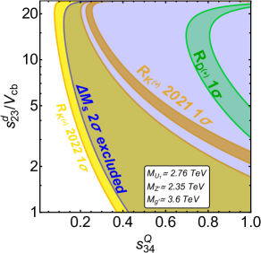
(a)

      

(b)

Figure 2.3: (Left) Regions compatible with $R_{D^{(*)}}$ and $R_{K^{(*)}}$ (2022 and 2021 data) in the plane ($s_{34}^{Q}$, $s_{23}^{d}$), the heavy gauge boson masses are fixed as depicted in the panel. (Right) Regions compatible with $R_{D^{(*)}}$ and $R_{K^{(*)}}$ (2022 and 2021 data) in the plane ($\left\langle\phi_{1}\right\rangle$,$\left\langle\phi_{3}\right\rangle$), which allows to explore the spectrum of heavy gauge boson masses. The mixing angles are fixed as depicted in the plot. In both panels the blue regions are excluded by the $\Delta M_{s}$ bound, see Eq. (D.24).

In Fig. 2.3b we have varied the VEVs of $\phi_{3}$ and $\phi_{1}$, effectively exploring the parameter space of gauge boson masses in line with Eq. (2.45). However, we find that the stringent constraints from $\Delta M_{s}$ are only alleviated when $\left\langle\phi_{3}\right\rangle\apprge 8\,\mathrm{TeV}$, which corresponds to a coloron with mass $M_{g^{\prime}}\gtrsim 50\,\mathrm{TeV}$ and a vector leptoquark with mass $M_{U_{1}}\apprge 34\,\mathrm{TeV}$, too heavy to address $R_{D^{(*)}}$.

We conclude that the model in this simplified version is over-constrained by large tree-level contributions to $\Delta M_{s}$ mediated by the coloron and $Z^{\prime}$. Such FCNCs arise due to the 2-3 CKM mixing having its origin in the down sector. Moreover, the same small 2-3 mixing angles suppress the contribution of the model to $R_{D^{(*)}}$. However, we shall show that the proper flavour structure to be compatible with all data is achieved in the extended version of the model presented in Section 3.

3 Extending the simplified twin Pati-Salam theory of flavour

In this section we present an extended version of the simplified twin Pati-Salam model, featuring extra matter content and a discrete flavour symmetry. This new version can achieve the proper flavour structure required to be compatible with all data, solving the problems of the simplified twin Pati-Salam model discussed in Section 2. Firstly, we will introduce the extended version of the model. Secondly, we will revisit the diagonalisation of the mass matrix, leading to the fermion masses and to the new couplings with the heavy gauge bosons. Finally, we will study the phenomenology, showing that the model is compatible with all data while predicting promising signals in flavour-violating observables, rare $B$-decays and high-$p_{T}$ searches.

3.1 New matter content and discrete flavour symmetry

As identified in DiLuzio:2018zxy , when one considers a 4321 model with all chiral fermions transforming as $SU(4)$ singlets (fermiophobic framework), three vector-like fermion families can achieve the proper flavour structure to explain the $B$-anomalies. Such flavour structure can provide a GIM-like suppression of FCNCs, along with large leptoquark couplings that can contribute to the LFU ratios. Hence, as depicted in Table 2, we extend now the simplified model by two extra vector-like families, to a total of three,

Field	$SU(4)_{PS}^{I}$	$SU(2)_{L}^{I}$	$SU(2)_{R}^{I}$	$SU(4)_{PS}^{II}$	$SU(2)_{L}^{II}$	$SU(2)_{R}^{II}$	$Z_{4}$
$\psi_{1,2,3}$	$\mathbf{1}$	$\mathbf{1}$	$\mathbf{1}$	$\mathbf{4}$	$\mathbf{2}$	$\mathbf{1}$	$\alpha$, 1, 1
$\psi_{1,2,3}^{c}$	$\mathbf{1}$	$\mathbf{1}$	$\mathbf{1}$	$\mathbf{\overline{4}}$	$\mathbf{1}$	$\mathbf{\overline{2}}$	$\alpha$, $\alpha^{2}$, 1
$\psi_{4,5,6}$	$\mathbf{4}$	$\mathbf{2}$	$\mathbf{1}$	$\mathbf{1}$	$\mathbf{1}$	$\mathbf{1}$	1, 1, $\alpha$
$\overline{\psi}_{4,5,6}$	$\mathbf{\overline{4}}$	$\mathbf{\overline{2}}$	$\mathbf{1}$	$\mathbf{1}$	$\mathbf{1}$	$\mathbf{1}$	1, 1, $\alpha^{3}$
$\psi_{4,5,6}^{c}$	$\mathbf{\overline{4}}$	$\mathbf{1}$	$\mathbf{\overline{2}}$	$\mathbf{1}$	$\mathbf{1}$	$\mathbf{1}$	1, 1, $\alpha$
$\overline{\psi^{c}}_{4,5,6}$	$\mathbf{4}$	$\mathbf{1}$	$\mathbf{2}$	$\mathbf{1}$	$\mathbf{1}$	$\mathbf{1}$	1, 1, $\alpha^{3}$
$\phi$	$\mathbf{4}$	$\mathbf{2}$	$\mathbf{1}$	$\mathbf{\overline{4}}$	$\mathbf{\overline{2}}$	$\mathbf{1}$	1
$\overline{\phi}$,$\,\overline{\phi^{\prime}}$	$\mathbf{\overline{4}}$	$\mathbf{1}$	$\mathbf{\overline{2}}$	$\mathbf{4}$	$\mathbf{1}$	$\mathbf{2}$	1, $\alpha^{2}$
$H$	$\mathbf{\overline{4}}$	$\mathbf{\overline{2}}$	$\mathbf{1}$	$\mathbf{4}$	$\mathbf{1}$	$\mathbf{2}$	1
$\overline{H}$	$\mathbf{4}$	$\mathbf{1}$	$\mathbf{2}$	$\mathbf{\overline{4}}$	$\mathbf{\overline{2}}$	$\mathbf{1}$	1
$H^{\prime}$	$\mathbf{1}$	$\mathbf{1}$	$\mathbf{1}$	$\mathbf{4}$	$\mathbf{1}$	$\mathbf{2}$	1
$\overline{H}^{\prime}$	$\mathbf{1}$	$\mathbf{1}$	$\mathbf{1}$	$\mathbf{\overline{4}}$	$\mathbf{1}$	$\mathbf{\overline{2}}$	1
$\Phi$	$\mathbf{1}$	$\mathbf{2}$	$\mathbf{1}$	$\mathbf{1}$	$\mathbf{\overline{2}}$	$\mathbf{1}$	1
$\overline{\Phi}$	$\mathbf{1}$	$\mathbf{1}$	$\mathbf{\overline{2}}$	$\mathbf{1}$	$\mathbf{1}$	$\mathbf{2}$	1
$\Omega_{15}$	$\mathbf{15}$	$\mathbf{1}$	$\mathbf{1}$	$\mathbf{1}$	$\mathbf{1}$	$\mathbf{1}$	1

Table 2: The field content under $G_{422}^{I}\times G_{422}^{II}\times Z_{4}$, see the main text for details.

$$\begin{array}[]{c}\psi_{4,5,6}(4,2,1;1,1,1)_{(1,1,\alpha)}\,,\overline{\psi}_{4,5,6}(\overline{4},\overline{2},1;1,1,1)_{(1,1,\alpha^{3})}\,,\\ \\ \psi_{4,5,6}^{c}(\overline{4},1,\overline{2};1,1,1)_{(1,1,\alpha)}\,,\overline{\psi^{c}}_{4,5,6}(4,1,2;1,1,1)_{(1,1,\alpha^{3})}\,,\end{array}$$ (3.1)

where it can be seen that all VL families originate from the first Pati-Salam group, being singlets under the second. They are indistinguishable under the twin Pati-Salam symmetry in Eq. (2.2), however a newly introduced $Z_{4}$ flavour symmetry discriminates the sixth family from the fourth and fifth, via different powers of the $Z_{4}$ charge $\alpha=e^{i\pi/2}$. This way, the total symmetry group of the high energy model is extended to

$$G_{422}^{I}\times G_{422}^{II}\times Z_{4}\,.$$ (3.2)

The new $Z_{4}$ discrete symmetry is introduced for phenomenological purposes, as it will prevent fine-tuning, reduce the total number of parameters of the model and protect from FCNCs involving the first family of SM-like chiral fermions. Moreover, $Z_{4}$ will simplify the diagonalisation of the full mass matrices and preserve the effective Yukawa couplings for SM fermions given in Section 2.3, with specific modifications. The origin of the chiral fermion families is still the second Pati-Salam group, however now they transform in a non-trivial way under $Z_{4}$,

$$\psi_{1,2,3}(1,1,1;4,2,1)_{(\alpha,1,1)}\,,\quad\psi_{1,2,3}^{c}(1,1,1;\overline{4},1,\overline{2})_{(\alpha,\alpha^{2},1)}\,.$$ (3.3)

Finally, the scalar content is extended by an additional scalar $\Omega_{15}$ which transforms in the adjoint representation of $SU(4)^{I}$, whose VEV $\left\langle\Omega_{15}\right\rangle=T_{15}v_{15}$ splits the vector-like masses, and

$$T_{15}=\frac{1}{2\sqrt{6}}\mathrm{diag}(1,1,1,-3)\,.$$ (3.4)

We also include an additional copy of the Yukon $\overline{\phi}$, denoted as $\overline{\phi^{\prime}}$, featuring $\alpha^{2}$ charge under $Z_{4}$. The simplified Lagrangian in Eq. (2.5) is extended by the new matter content to

$$\begin{aligned} \mathcal{L}_{\mathrm{mass}}^{ren}&=y_{ia}^{\psi}\overline{H}\psi_{i}\psi_{a}^{c}+y_{a3}^{\psi}H\psi_{a}\psi_{3}^{c}+x_{ia}^{\psi}\phi\psi_{i}\overline{\psi}_{a}+x_{a2}^{\psi^{c}}\overline{\psi_{a}^{c}\phi^{\prime}}\psi_{2}^{c}+x_{a3}^{\psi^{c}}\overline{\psi_{a}^{c}\phi}\psi_{3}^{c}+x_{16}^{\psi}\phi\psi_{1}\overline{\psi}_{6}+x_{61}^{\psi^{c}}\overline{\psi_{6}^{c}\phi}\psi_{1}^{c}&{}\\ {}&+M_{ab}^{\psi}\psi_{a}\overline{\psi_{b}}+M_{ab}^{\psi^{c}}\psi_{a}^{c}\overline{\psi_{b}^{c}}+M_{66}^{\psi}\psi_{6}\overline{\psi_{6}}+M_{66}^{\psi^{c}}\psi_{6}^{c}\overline{\psi_{6}^{c}}&{}\\ {}&+\lambda_{15}^{aa}\Omega_{15}\psi_{a}\overline{\psi_{a}}+\lambda_{15}^{66}\Omega_{15}\psi_{6}\overline{\psi_{6}}+\bar{\lambda}_{15}^{aa}\Omega_{15}\psi_{a}^{c}\overline{\psi_{a}^{c}}+\bar{\lambda}_{15}^{66}\Omega_{15}\psi_{6}^{c}\overline{\psi_{6}^{c}}+\mathrm{h.c.}\,,&{}\end{aligned}$$ (3.5)

where $i=2,3$ and $a,b=4,5$ (terms $i=1$ and $a,b=6$ forbidden by $Z_{4}$). The symmetry breaking and the decomposition of the different fields proceeds just like in the simplified model, see Section 2.2, however the VEVs of the additional scalars $\overline{\phi^{\prime}}$ and $\Omega_{15}$ play a role in the spontaneous breaking of the 4321 symmetry, and the corresponding gauge boson masses become (assuming $v_{1,3}\approx\overline{v}_{1,3}\approx\overline{v^{\prime}}_{1,3}$ for simplicity)

$$M_{U_{1}}=\frac{1}{2}g_{4}\sqrt{3v_{1}^{2}+3v_{3}^{2}+\frac{4}{3}v_{15}^{2}}\,,\quad M_{g^{\prime}}=\frac{\sqrt{3}}{\sqrt{2}}\sqrt{g_{4}^{2}+g_{3}^{2}}v_{3}\,,\quad M_{Z^{\prime}}=\frac{1}{2}\sqrt{\frac{3}{2}}\sqrt{g_{4}^{2}+\frac{2}{3}g_{1}^{2}}\sqrt{3v_{1}^{2}+v_{3}^{2}}\,.$$ (3.6)

3.2 Effective Yukawa couplings revisited

In this section, we diagonalise the full mass matrix of the extended model, following the same procedure as in Section 2.3, but including the extra matter content of the extended model. We may write the mass terms and couplings in Eq. (3.5) as a $9\times 9$ matrix in flavour space (we also define 9-dimensional vectors as $\psi_{\alpha}$ and $\psi_{\beta}^{c}$ below),

$$\mathcal{L}_{4,5,6}^{ren}=\psi_{\alpha}^{\mathrm{T}}M^{\psi}\psi_{\beta}^{c}+\mathrm{h.c.}\,,$$ (3.7)

$$\psi_{\alpha}=\left(\begin{array}[]{ccccccccc}\psi_{1}&\psi_{2}&\psi_{3}&\psi_{4}&\psi_{5}&\psi_{6}&\overline{\psi_{4}^{c}}&\overline{\psi_{5}^{c}}&\overline{\psi_{6}^{c}}\end{array}\right)^{\mathrm{T}}\,,\quad\psi_{\beta}^{c}=\left(\begin{array}[]{ccccccccc}\psi_{1}^{c}&\psi_{2}^{c}&\psi_{3}^{c}&\psi_{4}^{c}&\psi_{5}^{c}&\psi_{6}^{c}&\overline{\psi_{4}}&\overline{\psi_{5}}&\overline{\psi_{6}}\end{array}\right)^{\mathrm{T}}\,,$$ (3.8)

$$M^{\psi}=\left(\begin{array}[]{@{}llcccccccc@{}}&\lx@intercol\hfil\psi_{1}^{c}\hfil&\psi_{2}^{c}&\psi_{3}^{c}&\psi_{4}^{c}&\psi_{5}^{c}&\psi_{6}^{c}&\overline{\psi_{4}}&\overline{\psi_{5}}&\overline{\psi_{6}}\\ \cline{2-10}\cr\left.\psi_{1}\right|&0&0&0&0&0&0&0&0&x_{16}^{\psi}\phi\\ \left.\psi_{2}\right|&0&0&0&y_{24}^{\psi}\overline{H}&y_{25}^{\psi}\overline{H}&0&0&x_{25}^{\psi}\phi&0\\ \left.\psi_{3}\right|&0&0&0&y_{34}^{\psi}\overline{H}&y_{35}^{\psi}\overline{H}&0&x_{34}^{\psi}\phi&x_{35}^{\psi}\phi&0\\ \left.\psi_{4}\right|&0&0&y_{43}^{\psi}H&0&0&0&M_{44}^{Q,L}&M_{45}^{\psi}&0\\ \left.\psi_{5}\right|&0&0&y_{53}^{\psi}H&0&0&0&M_{54}^{\psi}&M_{55}^{Q,L}&0\\ \left.\psi_{6}\right|&0&0&0&0&0&0&0&0&M_{66}^{Q,L}\\ \left.\overline{\psi_{4}^{c}}\right|&0&x_{42}^{\psi^{c}}\overline{\phi^{\prime}}&x_{43}^{\psi^{c}}\overline{\phi}&M_{44}^{\psi^{c}}&M_{45}^{\psi^{c}}&0&0&0&0\\ \left.\overline{\psi_{5}^{c}}\right|&0&x_{52}^{\psi^{c}}\overline{\phi^{\prime}}&x_{53}^{\psi^{c}}\overline{\phi}&M_{54}^{\psi^{c}}&M_{55}^{\psi^{c}}&0&0&0&0\\ \left.\overline{\psi_{6}^{c}}\right|&x_{61}^{\psi^{c}}\overline{\phi}&0&0&0&0&M_{66}^{\psi^{c}}&0&0&0\end{array}\right)\,,$$ (3.9)

where the diagonal mass parameters $M_{44,55,66}^{Q,L}$ are splitted for quarks and leptons due to the VEV of $\Omega_{15}$,

$$M_{aa}^{Q}\equiv M_{aa}^{\psi}+\frac{\lambda_{15}^{aa}\left\langle\Omega_{15}\right\rangle}{2\sqrt{6}}\,,\quad M_{aa}^{L}\equiv M_{aa}^{\psi}-3\frac{\lambda_{15}^{aa}\left\langle\Omega_{15}\right\rangle}{2\sqrt{6}}\,,$$ (3.10)

where $a=4,5,6$. Similar equations are obtained for the $\psi^{c}$ sector, however in the $\psi^{c}$ sector the mass splitting is minimal due to $\left\langle\Omega_{15}\right\rangle$ being of order a few hundreds GeV while $M_{aa}^{\psi^{c}}$ are much heavier due to a generalisation of the hierarchy in Eq. (3.14). In Eq. (3.9) we have achieved an extra zero in the (2,7) entry by rotating $\psi_{2}$ and $\psi_{3}$, without loss of generality thanks to the zeros in the upper $3\times 3$ block (see Section 2.3).

The matrix in Eq. (3.9) features three different mass scales, the Higgs VEVs $\left\langle H\right\rangle$ and $\langle\overline{H}\rangle$, the Yukon VEVs $\left\langle\phi\right\rangle$, $\langle\overline{\phi}\rangle$, $\langle\overline{\phi^{\prime}}\rangle$ and the VL mass terms $M_{ab}^{\psi}$ and $M_{ab}^{\psi^{c}}$. We can block diagonalise the matrix above by taking advantage of the different mass scales. Firstly, we diagonalise the $2\times 2$ sub-blocks containing the heavy masses $M_{ab}^{\psi}$ and $M_{ab}^{\psi^{c}}$,

$$\left(\begin{array}[]{cc}M_{4}^{Q}&0\\ 0&M_{5}^{Q}\end{array}\right)=V_{45}^{Q}\left(\begin{array}[]{cc}M_{44}^{Q}&M_{45}^{\psi}\\ M_{54}^{\psi}&M_{55}^{Q}\end{array}\right)V_{45}^{\bar{Q}\dagger}\,,\qquad\left(\begin{array}[]{cc}M_{4}^{L}&0\\ 0&M_{5}^{L}\end{array}\right)=V_{45}^{L}\left(\begin{array}[]{cc}M_{44}^{L}&M_{45}^{\psi}\\ M_{54}^{\psi}&M_{55}^{L}\end{array}\right)V_{45}^{\bar{L}\dagger}\,,$$ (3.11)

and similarly in the $\psi^{c}$ sector. The 4-5 rotations above just redefine the elements in the 4th, 5th, 7th and 8th rows and columns of the full mass matrix, leaving the upper $3\times 3$ blocks unchanged (plus we reintroduce the zero in the (2,7) entry by another rotation of $\psi_{2}$ and $\psi_{3}$). Then we perform a further sequence of rotations to go to the decoupling basis, where no large elements appear apart from the diagonal heavy masses (i.e. those terms in the seventh, eighth and ninth rows and columns involving the fields $\phi$ and $\overline{\phi}$ are all absorbed into a redefinition of the heavy masses), and we obtain a block-diagonal matrix similar to that of Eq. (2.20) but enlarged with the fifth and sixth VL families. The total set of unitary transformations is given by

$$\begin{array}[]{c}V_{\psi}=V_{16}^{\psi}V_{35}^{\psi}V_{25}^{\psi}V_{34}^{\psi}V_{45}^{\psi}V_{45}^{\overline{\psi^{c}}}\,,\end{array}$$ (3.12)

$$V_{\psi^{c}}=V_{16}^{\psi^{c}}V_{35}^{\psi^{c}}V_{25}^{\psi^{c}}V_{34}^{\psi^{c}}V_{24}^{\psi^{c}}V_{45}^{\psi^{c}}V_{45}^{\bar{\psi}}\approx V_{34}^{\psi^{c}}V_{24}^{\psi^{c}}\,.$$ (3.13)

The mixing angles controlling the unitary transformations in Eq. (3.12) are given in Appendix A. The transformations in the $\psi^{c}$ sector of (3.13) can be described by $V_{34}^{\psi^{c}}V_{24}^{\psi^{c}}$ in good approximation, whose mixing angles are given by Eqs. (A.10) and (A.11). This approximation is accurate as far as the mixing involving the 5th and 6th $\psi^{c}$ fields is further suppressed by a generalisation of the hierarchy in Eq. (2.28) to three vector-like families, namely

$$M_{44}^{Q,L}\ll M_{55}^{Q,L}\sim M_{66}^{Q,L}\ll M_{44}^{\psi^{c}}\ll M_{55}^{\psi^{c}},M_{66}^{\psi^{c}}\,.$$ (3.14)

The hierarchy above will preserve most features of the basic simplified model, such as large third family Yukawa couplings arising from mixing with $\psi_{4}$ fermions, and small second family Yukawa couplings arising from mixing with $\psi_{4}^{c}$. The couplings of $U_{1}$ to chiral fermions will remain dominantly left-handed, since the couplings to $\psi^{c}$ chiral fermions (or equivalently right-handed fermions) will remain suppressed by small mixing angles. On the other hand, the hierarchy $M_{44}^{Q,L}\ll M_{55}^{Q,L}$ will provide hierarchical couplings of $U_{1}$ to third family and second family fermions, so we anticipate a small contribution to $R_{K^{(*)}}$ and a large contribution to $R_{D^{(*)}}$.

We obtain the effective Yukawa couplings for SM fermions by applying the set of unitary transformations in Eqs. (3.12) and (3.13) to the upper $6\times 6$ block of (2.19), in the same way as in Eq. (2.25). In this basis (primed), the mass matrix for each charged sector reads (assuming a small $x_{35}^{\psi}$, see Section 3.4.4 for the motivation, and approximating cosines in the $\psi^{c}$ sector to be 1),

$$M_{\mathrm{eff}}^{u}=\left(\begin{array}[]{@{}llcc@{}}&\lx@intercol\hfil\phantom{\!\,}u^{\prime}{}_{1}^{c}\hfil&\phantom{\!\,}u^{\prime}{}_{2}^{c}&\phantom{\!\,}u^{\prime}{}_{3}^{c}\\ \cline{2-4}\cr\left.Q^{\prime}_{1}\right|&0&0&0\\ \left.Q^{\prime}_{2}\right|&0&0&s_{25}^{Q}y_{53}^{\psi}\\ \left.Q^{\prime}_{3}\right|&0&0&s_{34}^{Q}y_{43}^{\psi}\end{array}\right)\left\langle H_{t}\right\rangle+\left(\begin{array}[]{@{}llcc@{}}&\lx@intercol\hfil\phantom{\!\,}u^{\prime}{}_{1}^{c}\hfil&\phantom{\!\,}u^{\prime}{}_{2}^{c}&\phantom{\!\,}u^{\prime}{}_{3}^{c}\\ \cline{2-4}\cr\left.Q^{\prime}_{1}\right|&0&0&0\\ \left.Q^{\prime}_{2}\right|&0&c_{25}^{Q}s_{24}^{q^{c}}y_{24}^{\psi}&c_{25}^{Q}s_{34}^{q^{c}}y_{24}^{\psi}\\ \left.Q^{\prime}_{3}\right|&0&c_{34}^{Q}s_{24}^{q^{c}}y_{34}^{\psi}&c_{34}^{Q}s_{34}^{q^{c}}y_{34}^{\psi}\end{array}\right)\left\langle H_{c}\right\rangle+\mathrm{h.c.}\,,$$ (3.15)

$$M_{\mathrm{eff}}^{d}=\left(\begin{array}[]{@{}llcc@{}}&\lx@intercol\hfil\phantom{\!\,}d^{\prime}{}_{1}^{c}\hfil&\phantom{\!\,}d^{\prime}{}_{2}^{c}&\phantom{\!\,}d^{\prime}{}_{3}^{c}\\ \cline{2-4}\cr\left.Q^{\prime}_{1}\right|&0&0&0\\ \left.Q^{\prime}_{2}\right|&0&0&s_{25}^{Q}y_{53}^{\psi}\\ \left.Q^{\prime}_{3}\right|&0&0&s_{34}^{Q}y_{43}^{\psi}\end{array}\right)\left\langle H_{b}\right\rangle+\left(\begin{array}[]{@{}llcc@{}}&\lx@intercol\hfil\phantom{\!\,}d^{\prime}{}_{1}^{c}\hfil&\phantom{\!\,}d^{\prime}{}_{2}^{c}&\phantom{\!\,}d^{\prime}{}_{3}^{c}\\ \cline{2-4}\cr\left.Q^{\prime}_{1}\right|&0&0&0\\ \left.Q^{\prime}_{2}\right|&0&c_{25}^{Q}s_{24}^{q^{c}}y_{24}^{\psi}&c_{25}^{Q}s_{34}^{q^{c}}y_{24}^{\psi}\\ \left.Q^{\prime}_{3}\right|&0&c_{34}^{Q}s_{24}^{q^{c}}y_{34}^{\psi}&c_{34}^{Q}s_{34}^{q^{c}}y_{34}^{\psi}\end{array}\right)\left\langle H_{s}\right\rangle+\mathrm{h.c.}\,,$$ (3.16)

$$M_{\mathrm{eff}}^{e}=\left(\begin{array}[]{@{}llcc@{}}&\lx@intercol\hfil\phantom{\!\,}e^{\prime}{}_{1}^{c}\hfil&\phantom{\!\,}e^{\prime}{}_{2}^{c}&\phantom{\!\,}e^{\prime}{}_{3}^{c}\\ \cline{2-4}\cr\left.L^{\prime}_{1}\right|&0&0&0\\ \left.L^{\prime}_{2}\right|&0&0&s_{25}^{L}y_{53}^{\psi}\\ \left.L^{\prime}_{3}\right|&0&0&s_{34}^{L}y_{43}^{\psi}\end{array}\right)\left\langle H_{\tau}\right\rangle+\left(\begin{array}[]{@{}llcc@{}}&\lx@intercol\hfil\phantom{\!\,}e^{\prime}{}_{1}^{c}\hfil&\phantom{\!\,}e^{\prime}{}_{2}^{c}&\phantom{\!\,}e^{\prime}{}_{3}^{c}\\ \cline{2-4}\cr\left.L^{\prime}_{1}\right|&0&0&0\\ \left.L^{\prime}_{2}\right|&0&c_{25}^{L}s_{24}^{e^{c}}y_{24}^{\psi}&c_{25}^{L}s_{34}^{e^{c}}y_{24}^{\psi}\\ \left.L^{\prime}_{3}\right|&0&c_{34}^{L}s_{24}^{e^{c}}y_{34}^{\psi}&c_{34}^{L}s_{34}^{e^{c}}y_{34}^{\psi}\end{array}\right)\left\langle H_{\mu}\right\rangle+\mathrm{h.c.}\,,$$ (3.17)

which are diagonalised by 2-3 rotations, and the CKM matrix is obtained via Eq. (2.33). The mass matrices above are of similar form to Eqs. (2.29), (2.30), (2.31), just featuring an extra off-diagonal component in the (2,3) entry of the first matrix in each sector, arising from mixing with the 5th family. This new term can be used to partially cancel the down 2-3 mixing while simultaneously enhancing up mixing to preserve the CKM, involving a mild tuning:

• Let us impose that the total (2,3) entry in the down quark mass matrix is small, i.e.

  $$-s_{25}^{Q}\left|y_{53}^{\psi}\right|\left\langle H_{b}\right\rangle+c_{25}^{Q}s_{34}^{q^{c}}y_{24}^{\psi}\left\langle H_{s}\right\rangle\approx 0\,.$$ (3.18)

  Following the discussion of Section 2.3, a natural benchmark is $\left\langle H_{b}\right\rangle\approx m_{b}$ and $s_{34}^{q^{c}}y_{24}^{\psi}\left\langle H_{s}\right\rangle\approx m_{s}$, hence

  $$-s_{25}^{Q}\left|y_{53}^{\psi}\right|m_{b}+m_{s}\approx 0\Longleftrightarrow\left|y_{53}^{\psi}\right|=\frac{m_{s}}{s_{25}^{Q}m_{b}}\,.$$ (3.19)

  On the other hand, the mixing angle $s_{25}^{Q}$ is very relevant for the $B$-decays and related phenomenology, and we obtain the typical value $s_{25}^{Q}\approx 0.2$ in Section 3.4, featuring another connection between the flavour puzzle and $B$-physics in our model. With this input, we obtain

  $$\left|y_{53}^{\psi}\right|\approx\mathcal{O}(0.1).$$ (3.20)

  In particular, the benchmark in Table 5 suppresses the down mixing with the choice $y_{53}^{\psi}=-0.3$, obtaining $s_{23}^{d}\approx\mathcal{O}(10^{-3})$ which is enough to control the stringent constraints from $B_{s}-\bar{B}_{s}$ meson mixing (see Section 2.4.2).

• At the same time that $y_{53}^{\psi}$ partially cancels the down mixing, it leads to large up mixing which preserves the CKM. Let us now estimate the 2-3 mixing in the up sector as the ratio of the (2,3) entry over the (3,3) entry in the up effective mass matrix,

  $$\frac{-s_{25}^{Q}\left|y_{53}^{\psi}\right|\left\langle H_{t}\right\rangle+c_{25}^{Q}s_{34}^{q^{c}}y_{24}^{\psi}\left\langle H_{c}\right\rangle}{s_{34}^{Q}y_{43}^{\psi}\left\langle H_{t}\right\rangle}\approx\frac{s_{25}^{Q}\left|y_{53}^{\psi}\right|\left\langle H_{t}\right\rangle+m_{c}}{m_{t}}\approx s_{25}^{Q}\left|y_{53}^{\psi}\right|\approx\mathcal{O}(V_{cb})\,,$$ (3.21)

  where we have considered $y_{43}^{\psi}=1$, $s_{34}^{Q}\approx 1$, as required to explain the top mass (see the discussion in the first bullet point of Section 2.3) and we have neglected the (2,3) term proportional to the smaller energy scale $\left\langle H_{c}\right\rangle$ when compared with the heavier $\left\langle H_{t}\right\rangle$. This way, we have taken advantage of the new contribution via the 5th family (and of the different hierarchies $m_{c}/m_{t}$ and $m_{s}/m_{b}$) to cancel the dangerous down mixing while preserving the CKM via up mixing.

• The situation in the lepton sector is similar due to Pati-Salam universality of the parameters, i.e.

  $$\frac{-s_{25}^{L}\left|y_{53}^{\psi}\right|\left\langle H_{\tau}\right\rangle+c_{25}^{L}s_{34}^{e^{c}}y_{24}^{\psi}\left\langle H_{\mu}\right\rangle}{s_{34}^{L}y_{43}^{\psi}\left\langle H_{\tau}\right\rangle}\approx\frac{-s_{25}^{L}\left|y_{53}^{\psi}\right|\left\langle H_{\tau}\right\rangle+m_{\mu}}{m_{\tau}}\approx s_{25}^{L}\left|y_{53}^{\psi}\right|\approx\mathcal{O}(V_{cb})\,.$$ (3.22)

  However, the leptonic mixing angles $s_{24}^{e^{c}}$ and $s_{34}^{e^{c}}$ are smaller than the quark ones due to the phenomenological relation $\left\langle\phi_{3}\right\rangle\gg\left\langle\phi_{1}\right\rangle$. This leads to $\left\langle H_{\mu}\right\rangle$ being above the scale of the muon mass, which predicts a quick growth of lepton mixing in the scenario $s_{34}^{e^{c}}>s_{24}^{e^{c}}$. This can be easily achieved in realistic benchmarks. In this scenario, interesting signals arise in LFV processes such as $\tau\rightarrow 3\mu$ or $\tau\rightarrow\mu\gamma$, mediated at tree-level by the $Z^{\prime}$ boson, see Section 3.4.5.

Other than the bullet points above, the mass matrices in Eqs. (3.15), (3.16), (3.17) lead to similar predictions as those of the simplified model in Section 2.3.

3.3 Vector-fermion interactions in the extended model

In this section we shall compute the vector-fermion couplings involving the heavy gauge bosons $U_{1}$, $g^{\prime}$, $Z^{\prime}$. The complete formulae can be found in Appendix B. We omit the couplings of the vector-like partners in the conjugate representations $\overline{\psi}_{\alpha}$ and $\overline{\psi_{\alpha}^{c}}$, since they do not mix with SM fermions.

3.3.1 $U_{1}$ couplings

In the original gauge basis, the vector leptoquark couples to the heavy EW doublets via the left-handed interactions,

$$\mathcal{L}_{U_{1}}^{\mathrm{gauge}}=\frac{g_{4}}{\sqrt{2}}\left(Q_{4}^{\dagger}\gamma_{\mu}L_{4}+Q_{5}^{\dagger}\gamma_{\mu}L_{5}+Q_{6}^{\dagger}\gamma_{\mu}L_{6}+\mathrm{h.c.}\right)U_{1}^{\mu}\,,$$ (3.23)

where similar couplings to the heavy EW singlets $\psi^{c}$ are also present, however they lead to suppressed couplings to SM fermions due to the hierarchy in Eq. (3.14). This way, we obtain purely left-handed $U_{1}$ couplings in good approximation. Now we shall apply the unitary transformations in Eq. (3.12) to rotate the fields from the original gauge basis to the decoupling basis (primed),

$$\mathcal{L}_{U_{1}}^{\mathrm{gauge}}=\frac{g_{4}}{\sqrt{2}}Q^{\prime}{}_{\alpha}^{\dagger}\gamma_{\mu}V_{Q}\gamma_{\mu}\mathrm{diag}(0,0,0,1,1,1)V_{L}^{\dagger}L^{\prime}_{\beta}U_{1}^{\mu}+\mathrm{h.c.}\,,$$ (3.24)

where

$$V_{Q}=V_{16}^{Q}V_{35}^{Q}V_{25}^{Q}V_{34}^{Q}V_{45}^{Q}\,,\qquad V_{L}=V_{16}^{L}V_{35}^{L}V_{25}^{L}V_{34}^{L}V_{45}^{L}\,.$$ (3.25)

The 4-5 rotations are different for quarks and leptons due to $\left\langle\Omega_{15}\right\rangle$ splitting the mass terms of the VL fermions. They lead to a non-trivial CKM-like matrix for the $U_{1}$ couplings,

$$W_{LQ}=V_{45}^{Q}V_{45}^{L\dagger}=\left(\begin{array}[]{ccc}c_{\theta_{LQ}}&-s_{\theta_{LQ}}&0\\ s_{\theta_{LQ}}&c_{\theta_{LQ}}&0\\ 0&0&1\end{array}\right)\,,$$ (3.26)

where $s_{\theta_{LQ}}$ depends on the angles $s_{45}^{Q}$ and $s_{45}^{L}$, obtained from the diagonalisation in Eq. (3.11). The unitary matrix $W_{LQ}$ can be regarded as a generalisation of the CKM matrix to $SU(4)$ or quark-lepton space. Similarly to the CKM case, the $W_{LQ}$ matrix is the only source of flavour-changing transitions among $SU(4)^{I}$ states, and it appears only in interactions mediated by $U_{1}$. In this sense, the vector leptoquark, $U_{1}$, is analogous to the SM $W^{\pm}$ bosons. Similarly, the $Z^{\prime}$, $g^{\prime}$ are analogous to the SM $Z$ boson, and we will show that their interactions are $SU(4)^{I}$ flavour-conserving at tree-level. In analogy to the SM, we will denote $U_{1}$ transitions as charged currents and $Z^{\prime}$, $g^{\prime}$ transitions as neutral currents. As in the SM, flavour-changing neutral currents (FCNCs) proportional to the $W_{LQ}$ matrix are generated at loop level. This mechanism was firstly identified in DiLuzio:2018zxy for a similar 4321 framework.

The same mixing that leads to the SM fermion masses and mixings, see Eq. (3.25), also leads to effective $U_{1}$ couplings to SM fermions which can contribute to the LFU ratios,

$$\mathcal{L}_{U_{1}}^{\mathrm{gauge}}=\frac{g_{4}}{\sqrt{2}}Q^{\prime}{}_{i}^{\dagger}\gamma_{\mu}\left(\begin{array}[]{ccc}s_{16}^{Q}s_{16}^{L}\epsilon&0&0\\ 0&c_{\theta_{LQ}}s_{25}^{Q}s_{25}^{L}&s_{\theta_{LQ}}s_{25}^{Q}s_{34}^{L}\\ 0&-s_{\theta_{LQ}}s_{34}^{Q}s_{25}^{L}&c_{\theta_{LQ}}s_{34}^{Q}s_{34}^{L}\end{array}\right)L^{\prime}_{j}U_{1}^{\mu}+\mathrm{h.c.}\,,$$ (3.27)

where we have considered that $s_{35}^{Q,L}$ are small, see Sections 3.2 and 3.4.4. The first family coupling can be diluted via mixing with vector-like fermions, which is parameterised via the effective parameter $\epsilon$ (see Appendix F for more details). The couplings above receive small corrections due to 2-3 fermion mixing arising after diagonalising the effective mass matrices in Eqs. (3.15), (3.16), (3.17). It can be seen from Eq. (3.27) that a large coupling (2,3) coupling $\beta_{c\nu_{\tau}}$ arises now, proportional to the large sines $s_{\theta_{LQ}}$, $s_{34}^{L}$ and $s_{25}^{Q}$. This solves one important issue of the simplified model, where the flavour-violating couplings $\beta_{c\nu_{\tau}}$ and $\beta_{b\mu}$ where connected to small 2-3 mixing angles, suppressing the contributions of $U_{1}$ to the LFU ratios. In any case, the leptoquark couplings that contribute to $B$-decays arise due to the same mixing effects which diagonalise the mass matrices of the model, yielding mass terms for the SM fermions. This way, the flavour puzzle and the $B$-anomalies are dynamically and parametrically connected in this model, leading to a predictive framework.

3.3.2 Coloron couplings and GIM-like mechanism

In the original gauge basis, the coloron couplings are flavour diagonal, featuring the following couplings to EW doublets,

$$\mathcal{L}_{g^{\prime}}^{\mathrm{gauge}}=\frac{g_{4}g_{s}}{g_{3}}\left(Q_{4}^{\dagger}\gamma^{\mu}T^{a}Q_{4}+Q_{5}^{\dagger}\gamma^{\mu}T^{a}Q_{5}+Q_{6}^{\dagger}\gamma^{\mu}T^{a}Q_{6}-\frac{g_{3}^{2}}{g_{4}^{2}}Q_{i}^{\dagger}\gamma^{\mu}T^{a}Q_{i}\right)g^{\prime}{}_{\mu}^{a}\,,$$ (3.28)

where $i=1,2,3$. Now we rotate to the decoupling basis by applying the transformations in Eq. (3.25), (assuming small $x_{35}^{\psi}$ as discussed in Section 3.4.4) obtaining

$$\mathcal{L}_{g^{\prime}}^{\mathrm{gauge}}=\frac{g_{4}g_{s}}{g_{3}}Q^{\prime}{}_{i}^{\dagger}\gamma^{\mu}T^{a}\left(\begin{array}[]{ccc}\left(s_{16}^{Q}\right)^{2}-\left(c_{16}^{Q}\right)^{2}\frac{g_{3}^{2}}{g_{4}^{2}}&0&0\\ 0&\left(s_{25}^{Q}\right)^{2}-\left(c_{25}^{Q}\right)^{2}\frac{g_{3}^{2}}{g_{4}^{2}}&0\\ 0&0&\left(s_{34}^{Q}\right)^{2}-\left(c_{34}^{Q}\right)^{2}\frac{g_{3}^{2}}{g_{4}^{2}}\end{array}\right)Q^{\prime}_{j}g^{\prime}{}_{\mu}^{a}\,,$$ (3.29)

Here $V_{45}^{Q}$ cancels due to unitarity and due to the $g^{\prime}$ couplings between VL quarks being flavour-universal in the original basis of (3.28). Therefore, as anticipated before, the CKM-like matrix $W_{LQ}$ does not affect the neutral currents mediated by $g^{\prime}$ (and similarly by $Z^{\prime}$). The coloron couplings in 3.29 receive small corrections due to 2-3 mixing arising after diagonalising the effective mass matrices in Eqs. (3.15), (3.16), (3.17), predominantly in the up sector, due to the down-aligned flavour structure achieved in Section 3.2. We obtain similar couplings for EW singlets, however their mixing angles are suppressed by the hierarchy in Eq. (3.14), and so they remain like in the original gauge basis.

The coloron couplings of Eq. (3.29) are flavour-universal if

$$s_{34}^{Q}=s_{25}^{Q}=s_{16}^{Q}\,,$$ (3.30)

leading to a GIM-like protection from tree-level FCNCs mediated by the coloron. The condition above was already identified in DiLuzio:2018zxy , denoted as full alignment limit. However, we have seen that maximal $s_{34}^{Q}\approx 1$ is well motivated in our model to protect the perturbativity of the top Yukawa, by the fit of the $R_{D^{(*)}}$ anomaly, and furthermore it naturally suppresses $s_{35}^{Q}$ via a small $c_{34}^{Q}$. The caveat is that if the condition in Eq. (3.30) is implemented, then $s_{16}^{Q}$ and $s_{25}^{Q}$ would also be maximal, leading to large couplings to valence quarks which would blow up the production of the coloron at the LHC. This fact was already identified in DiLuzio:2018zxy , where large $s_{34}^{Q}$ was also suggested by the $B$-anomalies, and a partial alignment limit was implemented,

$$s_{25}^{Q}=s_{16}^{Q}\,,$$ (3.31)

which suppresses FCNCs between the first and second quark families, proportional to the largest off-diagonal elements of the CKM matrix. FCNCs between the second and third families still arise, however we are protected from the stringent constraints of $B_{s}-\bar{B}_{s}$ meson mixing due to the down-aligned flavour structure achieved in Section 3.2. Finally, FCNCs between the first and third families are also under control, as they are proportional to the smaller elements of the CKM matrix.

The GIM-like condition of Eq. (3.31) translates, in terms of fundamental parameters of our model, into

$$\frac{x_{25}^{\psi}\left\langle\phi_{3}\right\rangle}{\sqrt{\left(x_{25}^{\psi}\left\langle\phi_{3}\right\rangle\right)^{2}+\left(M_{5}^{Q}\right)^{2}}}=\frac{x_{16}^{\psi}\left\langle\phi_{3}\right\rangle}{\sqrt{\left(x_{16}^{\psi}\left\langle\phi_{3}\right\rangle\right)^{2}+\left(M_{6}^{Q}\right)^{2}}}\,,$$ (3.32)

which could be naively achieved with natural couplings and $M_{5}^{Q}$, $M_{6}^{Q}$ being of the same order, as allowed by the messenger dominance in Eq. (3.14). The couplings and vector-like mass terms can also be chosen differently, as far as Eq. (3.32) is preserved. At the moment, the GIM-like mechanism is accidental. However, Eq. (3.32) suggests that the sixth and fifth family, and also the first and second families, might transform as doublets under a global $SU(2)$ symmetry, enforcing the parametric relations of Eq. (3.32).

A similar treatment of $Z^{\prime}$ couplings can be found in Appendix B, and a similar condition is obtained to suppress LFV between the first and second lepton families,

$$s_{25}^{L}=s_{16}^{L}\,.$$ (3.33)

Remarkably, if the condition of Eq. (3.31) is fulfilled, then Eq. (3.33) would also be fulfilled in good approximation thanks to the underlying twin Pati-Salam symmetry, the small breaking effects given by the splitting of VL masses via $\left\langle\Omega_{15}\right\rangle$.

3.4 Low-energy phenomenology

The twin PS model features a fermiophobic low-energy 4321 theory with a rich phenomenology. Although extensive analyses of general 4321 models have been performed during the last few years, the vast majority of them have been performed in the framework of non-fermiophobic 4321 models Cornella:2019hct ; Cornella:2021sby ; Barbieri:2022ikw ; Bordone:2017bld ; Bordone:2018nbg . Instead, the twin PS model offers a fermiophobic scenario with a different phenomenology. Being a theory of flavour, extra constraints and correlations arise via the generation of the SM Yukawa couplings and the prediction of fermion masses and mixing, including striking signals in LFV processes. Moreover, the underlying twin Pati-Salam symmetry introduces universality (and perturbativity) constraints over several parameters, which are not present in other models. These features motivate a dedicated analysis. We will highlight key observables for which the intrinsic nature of the model can be disentangled from all alternative proposals. All low-energy observables considered are listed in Table 3, with references to current experimental bounds and links to theory expressions.

Observable	Experiment/constraint	Theory expr.
$\left[C_{\nu edu}^{*}\right]^{3332}$ ($R_{D^{(*)}}$)	$0.07\pm 0.02$Angelescu:2021lln	(D.7)
$C_{9}^{\mu\mu}=-C_{10}^{\mu\mu}$ ($R_{K^{(*)}}^{2021}$)	$[-0.31,-0.48]$ (68% CL)Geng:2021nhg	(D.11)
$C_{9}^{\mu\mu}=-C_{10}^{\mu\mu}$ ($R_{K^{(*)}}^{2022}$)	$[-0.01,-0.14]$ (68% CL)(3.35)	(D.11)
$\delta(\Delta M_{s})$ ($B_{s}-\bar{B}_{s}$ mixing)	$\apprle 0.11$ (95% CL) DiLuzio:2019jyq	(D.25)
$\mathcal{B}\left(\tau\rightarrow 3\mu\right)$	$<2.1\cdot 10^{-8}$ (90% CL)Hayasaka:2010np	(D.34)
$\mathcal{B}\left(\tau\rightarrow\mu\gamma\right)$	$<5.0\cdot 10^{-8}$ (90% CL)HFLAV:2019otj	(D.42)
$\mathcal{B}\left(B_{s}\rightarrow\tau^{\pm}\mu^{\mp}\right)$	$<3.4\cdot 10^{-5}$ (90% CL)LHCb:2019ujz	(D.17)
$\mathcal{B}\left(B^{+}\rightarrow K^{+}\tau^{\pm}\mu^{\mp}\right)$	$<2.8\cdot 10^{-5}$ (90% CL)BaBar:2012azg	(D.18)
$\mathcal{B}\left(\tau\rightarrow\mu\phi\right)$	$<8.4\cdot 10^{-8}$ (90% CL)Belle:2011ogy	(D.35)
$\mathcal{B}\left(K_{L}\rightarrow\mu e\right)$	$<4.7\cdot 10^{-12}$ (90% CL) PDG:2022ynf	(3.43)
$(g_{\tau}/g_{e,\mu})_{\ell+\pi+K}$	$1.0003\pm 0.0014$ (68% CL)HFLAV:2022pwe	(3.44)
$\mathcal{B}\left(B_{s}\rightarrow\tau^{+}\tau^{-}\right)$	$<5.2\times 10^{-3}$ (90% CL)LHCb:2017myy	(D.14)
$\mathcal{B}\left(B\rightarrow K\tau^{+}\tau^{-}\right)$	$<2.25\times 10^{-3}$ (90% CL)BaBar:2016wgb	(D.15)
$\mathcal{B}\left(B\rightarrow K^{(*)}\nu\bar{\nu}\right)/\mathcal{B}\left(B\rightarrow K^{(*)}\nu\bar{\nu}\right)_{\mathrm{SM}}$	$<3.6\,(2.7)$ (90% CL)BaBar:2013npw ; Belle:2017oht	(3.45)

Table 3: Set of observables explored in the phenomenological analysis, including current experimental constraints.

The benchmark points BP1 and BP2 in Table 5 address the $R_{D^{(*)}}$ anomalies and are compatible with the 2021 and 2022 data on $R_{K^{(*)}}$, respectively, plus all the considered low-energy observables and high-$p_{T}$ searches. They provide a good starting point to study the relevant phenomenology, featuring typical configurations of the model, and allow us to confront the 2021 picture of the model versus the new situation with LFU preserved in $\mu/e$ ratios. Moreover, they fit second and third family charged fermion masses and mixings, featuring a down-aligned flavour structure with $\mathcal{O}(0.1)$ $\mu-\tau$ lepton mixing. The latter is more benchmark dependent, with the common range being $s_{23}^{e}=[V_{cb},5V_{cb}]$. The case $s_{23}^{e}\approx 0.1$ is interesting because it leads to intriguing signals in LFV processes, as we shall see. BP1 and BP2 also feature $x_{25}^{\psi}\approx x_{16}^{\psi}$ and $M_{5}^{Q,L}\approx M_{6}^{Q,L}$, providing a GIM-like suppression of 1-2 FCNCs.

In the forthcoming sections we will assume the couplings of the fundamental Lagrangian to be universal, such as $x_{34}^{\psi}$ and $x_{25}^{\psi}$, however their universality is broken by small RGE effects which we estimate in Section 3.4.8 to be below 8%. We neglect the small RGE effects and preserve universal parameters for the phenomenological analysis, in order to simplify the exploration of the parameter space and highlight the underlying twin Pati-Salam symmetry.

3.4.1 Model independent analysis of 2022 clean $b\rightarrow s\mu\mu$ data

This model was originally built to address and relate the 2021 $R_{K^{(*)}}$ and $R_{D^{(*)}}$ LFU anomalies, while connecting their origin to the origin of Yukawa couplings in the SM. This picture changed completely after the 2022 LHCb update of the $R_{K^{(*)}}$ ratios LHCb:2022qnv , which are now broadly compatible with the SM predictions (see Eq. (1.2)). New 2022 data of $\mathcal{B}(B_{s}\rightarrow\mu^{+}\mu^{-})$ by CMS Kar:2022tor is also compatible with the SM, while the previous measurements were hinting for values smaller than the SM prediction, including the 2021 measurement by LHCb LHCb:2021vsc . In our analysis, we will consider the global average of $\mathcal{B}(B_{s}\rightarrow\mu^{+}\mu^{-})$ experimental data by Allanach and Davighi Allanach:2022iod ,

Figure 3.1: Allowed regions in the plane $C_{9}^{\mu\mu}$ vs $C_{10}^{\mu\mu}$ to $1\sigma$ accuracy derived by using 2022 data on $R_{K}$ (blue region), $R_{K^{*}}$ (green region) and $\mathcal{B}(B_{s}\rightarrow\mu^{+}\mu^{-})$ (yellow region). The red contours denote the $1\sigma$, $2\sigma$ and $3\sigma$ regions of the $\chi^{2}$ fit. The black dot denotes the best fit point with $\Delta\chi^{2}/\mathrm{dof}\approx 0.56$.

$$\mathcal{B}(B_{s}\rightarrow\mu^{+}\mu^{-})=(3.28\pm 0.26)\times 10^{-9}\,,$$ (3.34)

which is roughly $1\sigma$ below the SM prediction $\mathcal{B}(B_{s}\rightarrow\mu^{+}\mu^{-})_{\mathrm{SM}}=(3.67\pm 0.15)\times 10^{-9}$. Instead, other observables such as the $B\rightarrow K\mu\mu$ Gubernari:2022hxn branching fraction and the angular observable $P^{\prime}_{5}$ LHCb:2020lmf ; LHCb:2020gog show important tensions with the SM, however such anomalies rely on important assumptions about the hadronic uncertainties, and their study is beyond the scope of this manuscript. Nonetheless, an extended discussion can be found in Section 3.4.3.

Following common practice, we describe $b\rightarrow s\mu\mu$ transitions in terms of the low-energy Lagrangian containing the usual $\mathcal{O}_{9}^{23\mu\mu}$ and $\mathcal{O}_{10}^{23\mu\mu}$ operators, defined in Eq. (D.10). More details and all the formulae are included in Appendix D.3. For the sake of clarity, we further simplify the notation by removing quark indexes and denote the corresponding NP Wilson coefficients (WCs) as $C_{9}^{\mu\mu}$ and $C_{10}^{\mu\mu}$. To the best of our knowledge, no explicit data for the theoretically clean fit of the WCs considering the new SM-like $R_{K^{(*)}}$ is given in the literature, motivating our own model independent analysis. The fits presented in the recent analyses Greljo:2022jac ; Ciuchini:2022wbq include observables which are not theoretically clean, and assumptions about the hadronic uncertainties need to be made. Instead, we need to explore how the theoretically clean, SM-like observables constrain the LFUV $C_{9}^{\mu\mu}=-C_{10}^{\mu\mu}$ which unavoidably arises in our model.

In Fig. 3.1 we show the parameter space in the plane ($C_{9}^{\mu\mu}$, $C_{10}^{\mu\mu}$) preferred by the 2022 $R_{K^{(*)}}$ ratios (in the central $q^{2}$) and the average of $\mathcal{B}(B_{s}\rightarrow\mu^{+}\mu^{-})$. We also display the result of a combined $\chi^{2}$ fit to all three observables as the red ellipses, denoting 1$\sigma$, $2\sigma$ and $3\sigma$ intervals. Our results show that a small but non-zero value of $C_{10}^{\mu\mu}$ is still preferred by $\mathcal{B}(B_{s}\rightarrow\mu^{+}\mu^{-})$. On the other hand, $C_{9}^{\mu\mu}$ is compatible with zero, but small positive and negative values are still allowed by the new $R_{K^{(*)}}$ ratios at $1\sigma$.

In particular, left-handed NP $C_{9}^{\mu\mu}=-C_{10}^{\mu\mu}$ are not far away from the $1\sigma$ region, and our 1-dimensional fit for the latter is

$$C_{9}^{\mu\mu}=-C_{10}^{\mu\mu}=[-0.0111,-0.1425]\>(1\sigma)\,,$$ (3.35)

with a best fit value of $C_{9}^{\mu\mu}=-C_{10}^{\mu\mu}=-0.0725$ with $\Delta\chi^{2}/\mathrm{dof}\approx 0.58$. Although left-handed NP are still allowed by the new data, the WCs are much smaller than those preferred by 2021 data (see Table 3).

In our model, the left-handed WC in Eq. (3.35) is obtained after integrating out the heavy gauge bosons, with the overall contribution being dominated by $U_{1}$ tree-level exchange. We shall constrain such contribution to the $\text{1}\sigma$ region in Eq. (3.35), and confront the new results against with the previous picture of 2021 data for which the model was developed.

3.4.2 $R_{D^{(*)}}$ and $R_{K^{(*)}}$

Beyond the contribution to $C_{9}^{\mu\mu}=-C_{10}^{\mu\mu}$ (see the EFT of the model in Appendix D.3), our model also generates a contribution to the WC $\left[C_{\nu edu}^{*}\right]^{3332}$ as defined in Appendix D.2. The latter contribution can accommodate existing tensions between the $R_{D^{(*)}}$ ratios and the SM. Namely, in terms of fundamental parameters of the model, the deviations from the SM of the LFU ratios scale as follows,

$$\left|\Delta R_{D^{(*)}}\right|\propto\left(x_{34}^{\psi}\right)^{3}x_{25}^{\psi}\,,$$ (3.36)

$$\left|\Delta R_{K^{(*)}}\right|\propto x_{34}^{\psi}\left(x_{25}^{\psi}\right)^{3}\,,$$ (3.37)

where we have fixed the VL masses and the 4321-breaking VEVs to the values of our benchmark (Table 5). This way, the Yukawa couplings above control the contributions to most of the relevant phenomenology, including the LFU ratios. The Pati-Salam universality of $x_{34}^{\psi}$ and $x_{25}^{\psi}$ provides here a welcome constraint, not present in other 4321 models. In particular, one can see that both $R_{D^{(*)}}$ and $R_{K^{(*)}}$ are connected via the same parameters and deviations in both are expected, while in other 4321 models the equivalent of $x_{i\alpha}^{\psi}$ decompose in different parameters for quarks and leptons, which decouple $R_{K^{(*)}}$ from $R_{D^{(*)}}$.

Following from Eqs. (3.36) and (3.37), the cubic dependence of $R_{K^{(*)}}$ on $x_{25}^{\psi}$ anticipates that we can suppress the contribution to $R_{K^{(*)}}$, while preserving a large contribution to $R_{D^{(*)}}$ thanks to its linear dependence on $x_{25}^{\psi}$. As a consequence, the yellow band of parameter space preferred by 2022 $R_{K^{(*)}}$ is just shifted below the orange band of 2021 $R_{K^{(*)}}$ in Fig. 3.3b. The 2022 $R_{K^{(*)}}$ band is compatible with $R_{D^{(*)}}$ at $1\sigma$ only in a narrow region of the parameter space. This is encouraging, given the fact that the model was built to address the 2021 tensions in both LFU ratios. However, in order to explain $R_{D^{(*)}}$, small deviations from the SM in the $R_{K^{(*)}}$ ratios are unavoidable, to be tested in the future via more precise measurements of LFU by the LHCb collaboration. Moreover, lower central values for $R_{D^{(*)}}$ are also expected.

Remarkably, the fact that the twin PS model only generates the effective operator $(\bar{c}_{L}\gamma_{\mu}b_{L})$ $(\bar{\text{$\tau$}}_{L}\gamma^{\mu}\nu_{\tau L})$ implies that both $R_{D}$ and $R_{D^{*}}$ are corrected in the same direction and with the same size. Instead, non-fermiophobic 4321 models also predict the scalar operator $(\bar{c}_{L}b_{R})(\bar{\text{$\tau$}}_{R}\nu_{\tau L})$, which leads to a larger correction of $R_{D}$ than that of $R_{D^{*}}$ (about 5/2 larger for the $\mathrm{PS}^{3}$ model, see Eq. (27) in Bordone:2017bld ).

3.4.3 Off-shell photon penguin with tau leptons

The explanation of $R_{D^{(*)}}$ in our model is correlated to new contributions to $b\rightarrow s\tau\tau$ due to $SU(2)_{L}$ invariance of the $U_{1}$ couplings, to be explored in detail in Section 3.4.7. Interestingly, the same couplings that contribute to $b\rightarrow s\tau\tau$ also lead to an off-shell photon penguin diagram with tau leptons running in the loop, which generates a lepton universal contribution to the operator $\mathcal{O}_{9}^{23\ell\ell}=(\bar{s}_{L}\gamma_{\mu}b_{L})(\bar{\ell}\gamma^{\mu}\ell)$ entering in $b\rightarrow s\ell\ell$ transitions, namely

(a)

      

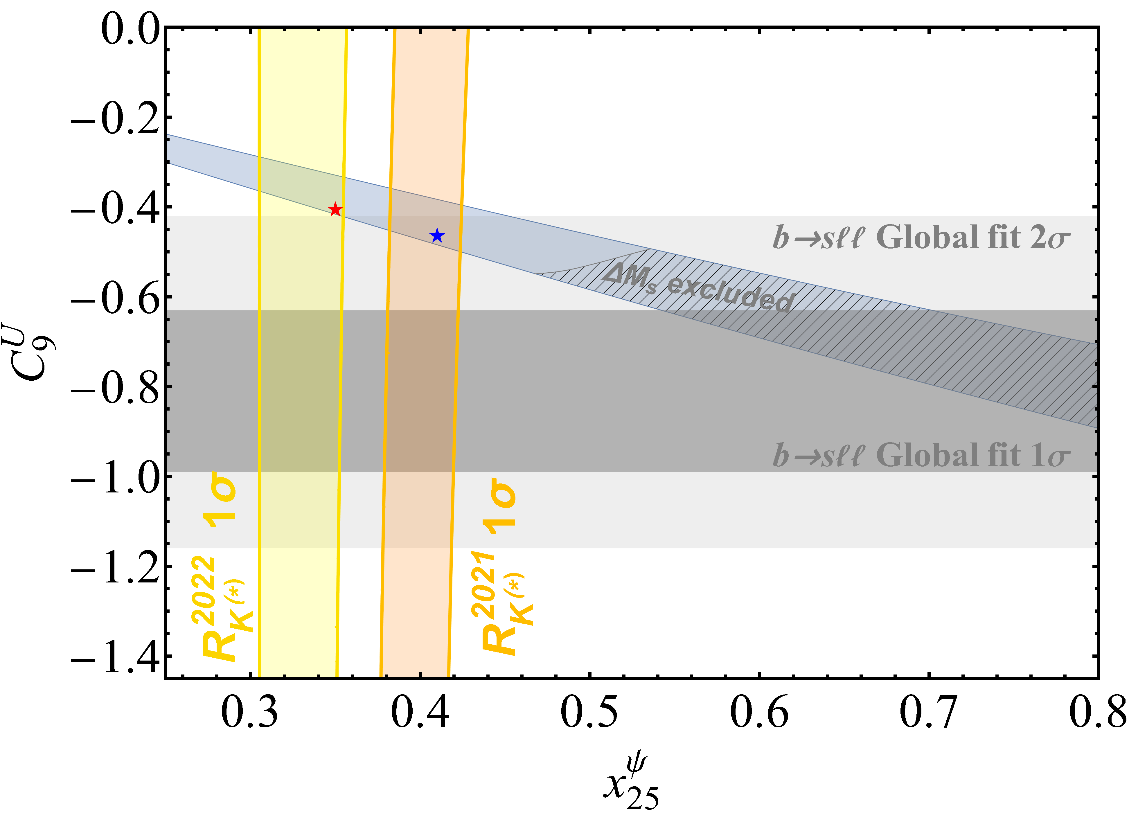
(b)

Figure 3.2: (Left) Off-shell photon penguin with tau leptons in the loop that generates $C_{9}^{U}$, a contribution to the lepton universal operator $\mathcal{O}_{9}^{23\ell\ell}$ that participates in $b\rightarrow s\ell\ell$ transitions. (Right) $C_{9}^{U}$ as a function of $x_{25}^{\psi}$ via Eq. (3.38), with $x_{34}^{\psi}$ varied in the range [1, 3.5] as preferred by $R_{D^{(*)}}$ (blue region), with the rest of parameters fixed as in Table 5. The gray (light gray) region denotes the 1$\sigma$ ($2\sigma$) contour of $C_{9}^{U}$ as preferred by a global fit to $b\rightarrow s\ell\ell$ data taken from Alguero:2021anc . The yellow (orange) band denotes the $1\sigma$ region preferred by $R_{K^{(*)}}^{2022}$ ($R_{K^{(*)}}^{2021}$). The blue and red stars denote BP1 and BP2 respectively.

$$C_{9}^{U}=-\frac{v_{\mathrm{SM}}^{2}g_{4}^{2}}{6V_{tb}V_{ts}^{*}M_{U_{\text{1}}}^{2}}\left(\log\left[\frac{2m_{b}^{2}}{g_{4}^{2}M_{U_{1}}^{2}}\right]\beta_{s\tau}\beta_{b\tau}^{*}+\log\left[\frac{2m_{E_{5}}^{2}}{g_{4}^{2}M_{U_{1}}^{2}}\right]\beta_{sE_{5}}\beta_{bE_{5}}^{*}+\log\left[\frac{2m_{E_{4}}^{2}}{g_{4}^{2}M_{U_{1}}^{2}}\right]\beta_{sE_{4}}\beta_{bE_{4}}^{*}\right)\,,$$ (3.38)

which is explicitly correlated to $b\rightarrow s\tau\tau$, as well as to $R_{D^{(*)}}$ since $SU(2)_{L}$ invariance implies $\beta_{s\tau}\approx\beta_{c\nu_{\tau}}$ for the $U_{1}$ couplings. Therefore, the scaling is $|C_{9}^{U}|\propto(x_{34}^{\psi})^{3}x_{25}^{\psi}$, just like $R_{D^{(*)}}$. A similar contribution has been studied in the literature in a model independent framework Bobeth:2014rda ; Capdevila:2017iqn ; Crivellin:2018yvo ; Alguero:2022wkd , however in our model we need to add the contributions via the extra VL charged leptons $E_{4,5}$, see Fig. 3.2a. Unfortunately, due to the flavour structure of our model, the contributions via VL leptons interfere negatively with the leading contribution via the tau loop, and hence our overall contribution to $C_{9}^{U}$ is smaller than in other models. The contribution from $E_{4}$ is negligible, but the contribution from $E_{5}$ reduces $C_{9}^{U}$ by a 20% factor of the tau loop contribution.

In our model, $R_{D^{(*)}}$ and $R_{K^{(*)}}$ are correlated, as can be seen from Eqs. (3.36) and (3.37). Therefore, $C_{9}^{U}$ is not only correlated with $R_{D^{(*)}}$ but also with $R_{K^{(*)}}$. Given that deviations from 1 in $R_{K^{(*)}}$ are now constrained by the new LHCb measurements, our final contribution to $C_{9}^{U}$ is constrained to be $C_{9}^{U}\approx-0.4$, as can be seen in Fig. 3.2b. However, global fits of $b\rightarrow s\ell\ell$ data (see e.g. Alguero:2021anc ; Greljo:2022jac ; Ciuchini:2022wbq ), mostly driven by anomalies in $\mathrm{Br}(B\rightarrow K\mu\mu)$, $\mathrm{Br}(B_{s}\rightarrow\phi\mu\mu)$ and $P^{\prime}_{5}(B\rightarrow K^{*}\mu\mu)$ (see e.g. Gubernari:2022hxn ), prefer a larger value $C_{9}^{U}\approx-0.8$. Therefore, we conclude that our model is not able to fully address the anomalies in $b\rightarrow s\ell\ell$ via the off-shell photon penguin, although our contribution to $C_{9}^{U}$ ameliorates the tensions. Performing a more ambitious analysis would require to make assumptions about the hadronic uncertainties afflicting $\mathrm{Br}(B\rightarrow K\mu\mu)$, $\mathrm{Br}(B_{s}\rightarrow\phi\mu\mu)$ and $P^{\prime}_{5}(B\rightarrow K^{*}\mu\mu)$, which is beyond the scope of this paper.

3.4.4 $B_{s}-\bar{B}_{s}$ mixing

In the twin PS model as presented in Section 3, tree-level contributions to $B_{s}-\bar{B}_{s}$ mixing via 2-3 quark mixing are suppressed due to the down-aligned flavour structure achieved in Section 3.2. A further 1-loop contribution mediated by $U_{1}$ has been studied in the literature DiLuzio:2018zxy ; Cornella:2021sby ; Fuentes-Martin:2020hvc for other 4321 models, and vector-like charged leptons are known to play a crucial role. In DiLuzio:2018zxy a framework with three VL charged leptons was considered, however the loop function was generalised from the SM $W$ box, so the bounds where expected to be slightly overestimated. Instead, in Fuentes-Martin:2020hvc the proper loop function was derived, but a framework with only one VL charged lepton was considered. For this work, we have generalised the loop function of Fuentes-Martin:2020hvc to the case of three VL leptons. The 1-loop contribution mediated by $U_{1}$ reads,

$$C_{bs}^{\mathrm{NP-loop}}=\frac{g_{4}^{4}}{\left(8\pi M_{U_{1}}\right)^{2}}\sum_{\alpha,\beta}\left(\beta_{s\alpha}^{*}\beta_{b\alpha}\right)\left(\beta_{s\beta}^{*}\beta_{b\beta}\right)F(x_{\alpha},x_{\beta})\,,$$ (3.39)

where $\alpha,\beta=\mu,\tau,E_{4},E_{5}$ run for all charged leptons, including the vector-like partners (except for electrons and the sixth charged lepton which do not couple to the second or third generation), and $x_{\alpha}=(m_{\alpha}/M_{U_{1}})^{2}$. The contribution corresponds to the box diagrams in Fig. D.1. The proper loop function for our framework is given in Appendix D.4.1.

The product of couplings $\beta_{s\alpha}^{*}\beta_{b\alpha}$ has the fundamental property

$$\sum_{\alpha}\beta_{s\alpha}^{*}\beta_{b\alpha}=0\,,$$ (3.40)

which arises trivially from unitarity of the transformations in Eq. (3.25). This property, similarly to the GIM mechanism in the SM, is essential to render the loop finite. However, the property holds as long as the 2-3 down mixing and $s_{35}^{Q}$ are small. In particular, $s_{35}^{Q}$ is naturally small in the scenario $s_{34}^{Q}\approx 1$, as it is suppressed by the small cosine $c_{34}^{Q}$, see the definition of $s_{35}^{Q}$ in Eq. (A.8). Ultimately, the mixing angle $s_{35}^{Q}$ is controlled by the fundamental parameter $x_{35}^{\psi}$, and we obtained that $x_{35}^{\psi}\apprle 0.09$ is required to survive the $\Delta M_{s}$ bound.

The loop function is dominated by the heavy vector-like partners. In particular, in the motivated scenario with maximal $s_{34}^{L}$, the couplings with the fourth family $\beta_{sE_{4}}^{*}\beta_{bE_{4}}$ are suppressed by the small cosine $c_{34}^{L}$. This way, the loop is dominated by $E_{5}$ in good approximation, and we can apply the property (3.40) to obtain

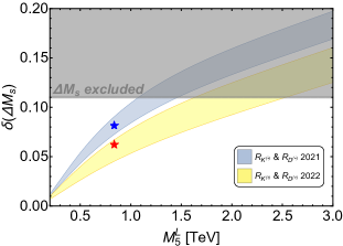
(a)

      

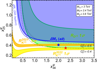
(b)

Figure 3.3: (Left) $\delta(\Delta M_{s})$ (Eq. (D.25)) as a function of the 5th vector-like mass term. $x_{25}^{\psi}$ is varied in the range $x_{25}^{\psi}=[0.3,\,0.35]$ ($[0.4,\,0.45]$) preferred by $R_{K^{(*)}}^{2022}$ ($R_{K^{(*)}}^{2021}$ ), obtaining the yellow (blue) band. The gray region is excluded by the $\Delta M_{s}$ bound, see Eq. (D.24). (Right) Parameter space in the plane ($x_{34}^{\psi}$, $x_{25}^{\psi}$) compatible with $R_{D^{(*)}}$ and $R_{K^{(*)}}$ at 1$\sigma$. The remaining parameters are fixed as in Table 5 for both panels. The dashed lines show contours of constant $C_{9}^{U}$. The blue region is excluded by the $\Delta M_{s}$ bound, the region excluded only due to the contribution via the 5th lepton is also shown in lighter blue for comparison. The blue and red stars denote BP1 and BP2 respectively.

$$C_{bs}^{\mathrm{NP-loop}}=\frac{g_{4}^{4}}{\left(8\pi M_{U_{1}}\right)^{2}}\left(\beta_{sE_{5}}^{*}\beta_{bE_{5}}\right)^{2}\tilde{F}(x_{E_{5}})\,.$$ (3.41)

The loop function grows with $x_{E_{5}}$ (see Appendix D.4.1). However, in the limit of large bare mass term $M_{5}^{L}$ the effective coupling $\beta_{sE_{5}}^{*}\propto s_{25}^{Q}$ vanishes (since large $M_{5}^{L}$ also implies large $M_{5}^{Q}$ due to the Pati-Salam symmetry), hence both the contribution to $\Delta M_{s}$ and $R_{D^{(*)}}$ go away. In Fig. 3.3a we plot $\delta(\Delta M_{s})$ defined in Eq. (D.25) in terms of $M_{5}^{L}$, and we vary $x_{25}^{\psi}$ in the ranges compatible with $R_{D^{(*)}}$ and $R_{K^{(*)}}^{2022}$ ($R_{K^{(*)}}^{2021}$). We can see that the $\Delta M_{s}$ bound requires a vector-like lepton around 1.5-2 TeV in the 2022 case, while 2021 data was pointing to a VL lepton with a mass around 1 TeV.

In Fig. 3.3b we show that Eq. (3.41) is indeed a good approximation, up to small interference effects between the 4th and 5th family contributions in the small $x_{34}^{\psi}$ region, where the fourth lepton is lighter. We also show the parameter space compatible with $\Delta M_{s}$ and the LFU ratios in our benchmark scenario. In particular, $\Delta M_{s}$ turns out to be the largest constraint over the parameter space other than $R_{K^{(*)}}^{2022}$.

3.4.5 LFV processes

$\boldsymbol{\tau\rightarrow 3\mu}$

The partial alignment condition of Eq. (3.33) allows for $Z^{\prime}$-mediated FCNCs in $\tau\mu$ processes, due to the fact that the model predicts significant mixing between the muon and tau leptons. This is a crucial prediction of the twin PS theory of flavour, not present in general 4321 models. Of particular interest is the process $\tau\rightarrow 3\mu$, which receives a tree-level $Z^{\prime}$ contribution that grows with the $\tau\mu$ mixing angle $s_{23}^{e}$. Beyond the latter, $\tau\rightarrow 3\mu$ also receives a $U_{1}$-mediated 1-loop contribution

$$C_{\tau\mu\mu\mu}^{U_{1}}=\frac{3g_{4}^{4}}{128\pi^{2}M_{U_{1}}^{2}}\beta_{D_{5}\mu}^{*}\beta_{D_{5}\tau}\left(\beta_{D_{5}\mu}\right)^{2}\tilde{F}(x_{D_{5}})\,.$$ (3.42)

The effective coupling $\beta_{D_{5}\mu}$ is proportional to $s_{25}^{L}\approx 0.1$, which provides a further suppression of $\mathcal{O}((s_{25}^{L})^{3})$ that renders the loop negligible against the much larger tree-level $Z^{\prime}$-mediated contribution. The typical benchmark $s_{25}^{L}\approx 0.1$ naturally suppresses the $\mu\mu Z^{\prime}$ coupling, keeping the $Z^{\prime}$ contribution to $\tau\rightarrow 3\mu$ under control, and simultaneously protects from $Z^{\prime}\rightarrow\mu\mu$ at LHC (see Section 3.4.9).

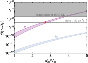
(a)

      

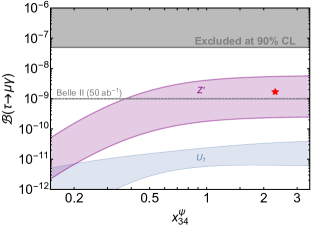
(b)

Figure 3.4: (Left) $\mathcal{B}\left(\tau\rightarrow 3\mu\right)$ as a function of the 2-3 charged lepton mixing sine $s_{23}^{e}$. The purple region denotes the $Z^{\prime}$ contribution while the blue region denotes the $U_{1}$ contribution, for both we have varied $x_{25}^{\psi}=[0.3,0.35]$ which is compatible with $R_{K^{(*)}}^{2022}$. (Right) $\mathcal{B}\left(\tau\rightarrow\mu\gamma\right)$ as a function of $x_{34}^{\psi}$. The purple region denotes the $Z^{\prime}$ contribution for which we have varied $s_{23}^{e}=[V_{cb},5V_{cb}]$. The blue region denotes the $U_{1}$ contribution, for which we have varied $x_{25}^{\psi}=[0.1,1]$. The gray regions are excluded by the experiment, the dashed lines show the projected future bound. The red star shows BP2.

As depicted in Fig. 3.4a, the $Z^{\prime}$ contribution dominates over the $U_{1}$ contribution, and the regions of the parameter space with very large $s_{23}^{e}$ are already excluded by the experiment. We have chosen to plot the results of the 2022 case only, since this observable depends mostly on $s_{23}^{e}$ and there is little variation with 2021 data. The Belle II collaboration will test a further region of the parameter space Belle-II:2018jsg , setting the bound $s_{23}^{e}<2.8V_{cb}$ if no signal is detected. In all UV incomplete 4321 models (such as DiLuzio:2017vat ; DiLuzio:2018zxy ) the $\mu-\tau$ mixing is unspecified, so only the small $U_{1}$ signal is predicted. Therefore, the large $Z^{\prime}$ signal offers the opportunity to disentangle the twin Pati-Salam model from other 4321 proposals.

As depicted in Fig. 3.5b, $\tau\rightarrow 3\mu$ is the most constraining signal over the parameter space out of all the LFV processes, provided that the 2-3 charged lepton mixing is $\mathcal{O}(0.1)$.

$\boldsymbol{\tau\rightarrow\mu\gamma}$

The process $\tau\rightarrow\mu\gamma$ receives 1-loop contributions via both $Z^{\prime}$ and $U_{1}$, as depicted in Fig. D.2, with formulae reported in Appendix D.5.1. Provided that the 3-4 mixing is maximal, the $U_{1}$ loop is dominated by the 5th vector-like quark, and in this situation the couplings $\beta_{D_{5}\mu}^{*}\beta_{D_{5}\tau}$ are controlled by $x_{25}^{\psi}$. The $Z^{\prime}$ loop is dominated by chiral leptons, in particular by the $\tau$ lepton, since the coupling $\xi_{\tau\tau}$ is maximal while $\xi_{\mu\mu}$ is suppressed. In this scenario, the overall $Z^{\prime}$ contribution is controlled by $\xi_{\tau\mu}$ which grows with the $\mu-\tau$ mixing angle $s_{23}^{e}$, and the variation via $x_{25}^{\psi}$ is minimal.

In Fig. 3.4b we can see that the $Z^{\prime}$ contribution dominates the branching fraction in the range of large $x_{34}^{\psi}$ motivated by $R_{D^{(*)}}$, leading to the predictions for $\mathcal{B}\left(\tau\rightarrow\mu\gamma\right)$ being one/three orders of magnitude below the current experimental limit depending on the value of $s_{23}^{e}$. We have also included the projected bound by Belle II (50 $\mathrm{ab^{-1}}$) Belle-II:2018jsg , which will partially test the parameter space. In the 4321 models of DiLuzio:2017vat ; DiLuzio:2018zxy the $\mu-\tau$ mixing is unspecified, so only the blue $U_{1}$ signal is predicted. For non-fermiophobic models, this signal is largely enhanced via a chirality flip with the bottom quark running in the loop Cornella:2019hct ; Cornella:2021sby ; Barbieri:2022ikw ; Fuentes-Martin:2020bnh ; Fuentes-Martin:2020hvc , predicting a larger signal $\mathcal{B}\left(\tau\rightarrow\mu\gamma\right)\approx 10^{-8}$. Instead, our $Z^{\prime}$ signal lies below, offering the opportunity to disentangle the twin Pati-Salam model from all other proposals.

$\boldsymbol{B_{s}\rightarrow\tau\mu}$, $\boldsymbol{B\rightarrow K\tau\mu}$ and $\boldsymbol{\tau\rightarrow\mu\phi}$

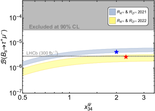
(a)

      

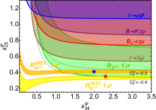
(b)

Figure 3.5: (Left) $\mathcal{B}\left(B_{s}\rightarrow\tau^{+}\mu^{-}\right)$ as a function of $x_{34}^{\psi}$. The yellow (blue) band is obtained by varying $x_{25}^{\psi}$ in the range $x_{25}^{\psi}=[0.3,\,0.35]$($[0.4,\,0.45]$) preferred by $R_{K^{(*)}}^{2022}$ ($R_{K^{(*)}}^{2021}$ ). The gray region is excluded by the experiment, the dashed line shows the projected future bound. (Right) Parameter space in the plane ($x_{34}^{\psi}$, $x_{25}^{\psi}$) compatible with $R_{D^{(*)}}$ and $R_{K^{(*)}}$ at 1$\sigma$. The remaining parameters are fixed as in Table 5. The dashed lines show contours of constant $C_{9}^{U}$. The regions excluded by LFV violating processes are displayed. The blue (red) star shows BP1 (BP2).

The vector leptoquark $U_{1}$ mediates tree-level contributions to flavour-violating (semi)leptonic $B$-decays to (kaons), taus and muons. The experimental bound for $B_{s}\rightarrow\tau\mu$ was obtained by LHCb LHCb:2019ujz , while for $B\rightarrow K\tau\mu$ experimental bounds are only available for the decays $B^{+}\rightarrow K^{+}\tau\mu$ BaBar:2012azg . The process $\tau\rightarrow\mu\phi$ receives tree-level contributions from both $U_{1}$ and $Z^{\prime}$, see Appendix D.3 and D.5. However, $\tau\rightarrow\mu\phi$ turns out to be suppressed by the small effective couplings $\beta_{s\mu}\propto s_{25}^{Q}s_{25}^{L}$ and $\xi_{ss}\propto\left(s_{25}^{Q}\right)^{2}$ and we find $\mathcal{B}\left(\tau\rightarrow\mu\phi\right)\approx 10^{-9}$, roughly two orders of magnitude below the current experimental bounds, and just below the future sensitivity of Belle II.

As can be seen in Fig. 3.5b, $B_{s}\rightarrow\tau^{+}\mu^{-}$ implies the largest constraint over the parameter space out of all semileptonic LFV processes involving $\tau$ leptons, followed by $B^{+}\rightarrow K^{+}\tau^{+}\mu^{-}$ and $\tau\rightarrow\mu\phi$. The present experimental bounds lead to mild constraints over the parameter space compatible with $R_{D^{(*)}}$. As depicted in Fig. 3.5a, the 2021 region for $B_{s}\rightarrow\tau^{+}\mu^{-}$ was partially within LHCb projected sensitivity, but the 2022 region will mostly remain untested.

$\boldsymbol{K_{L}\rightarrow\mu e}$

The LFV process $K_{L}\rightarrow\mu e$ sets a strong constraint over all models featuring a vector leptoquark $U_{1}$ with first and second family couplings Dolan:2020doe ,

$$\mathcal{B}\left(K_{L}\rightarrow\mu e\right)=\frac{\tau_{K_{L}}G_{F}^{2}f_{K}^{2}m_{\mu}^{2}m_{K}}{8\pi}\left(1-\frac{m_{\mu}^{2}}{m_{K}^{2}}\right)^{2}C_{U}^{2}\left|\beta_{de}\beta_{s\mu}^{*}\right|^{2}\,.$$ (3.43)

The first family coupling $\beta_{de}$ can be diluted via mixing with vector-like fermions, which we parameterised via the effective parameter $\epsilon$ in Eq. (3.27), so that $\beta_{se}\approx s_{16}^{Q}s_{16}^{L}\epsilon$. The mechanism to perform this and the definition of $\epsilon$ in terms of fundamental parameters of the model is included in Appendix F.

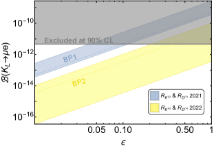
(a)

      

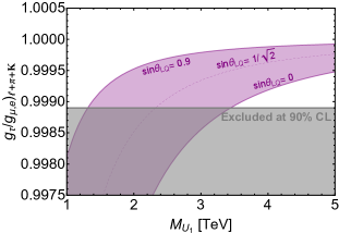
(b)

Figure 3.6: (Left) $\mathcal{B}\left(K_{L}\rightarrow\mu e\right)$ (Eq. (3.43)) as a function of $\epsilon$ (see main text for details). $x_{25}^{\psi}$ is varied in the range $x_{25}^{\psi}=[0.3,\,0.35]$ ($[0.4,\,0.45]$) preferred by $R_{K^{(*)}}^{2022}$ ($R_{K^{(*)}}^{2021}$ ), obtaining the yellow (blue) band. (Right) LFU ratios originated from $\tau$ decays (Eq. (3.44)) as a function of the mass of the vector leptoquark $M_{U_{1}}$, $\sin\theta_{LQ}$ is varied in the range $\sin\theta_{LQ}=[0,0.9]$ and $g_{4}=3.5$. The remaining parameters are fixed as in Table 5 for both panels, and current exclusion limits are shown.

In Fig. 3.6a we can see that for the 2022 case, some region of the parameter space is compatible with $K_{L}\rightarrow\mu e$ without the need of diluting the coupling. Instead, for the benchmark values BP1 and BP2, a mild suppression is required. In Appendix F, a benchmark with the fundamental parameters of the model that provide such a suppression is included. This signal is a direct consequence of the underlying twin PS symmetry and the GIM-like mechanism, which lead to quasi-degenerate mixing angles $s_{16}^{Q}\approx s_{16}^{L}$ that are equal to their 25 counterparts, and as a consequence $\beta_{de}\neq 0$. Therefore, it is not present in other 4321 models DiLuzio:2017vat ; DiLuzio:2018zxy ; Cornella:2019hct ; Cornella:2021sby ; Barbieri:2022ikw .

3.4.6 Tests of universality in leptonic $\tau$ decays

NP contributions to $R_{D^{(*)}}$ commonly involve large couplings to $\tau$ leptons, which can have an important effect over LFU ratios originated from $\tau$ decays. Such tests are constructed by performing ratios of the partial widths of a lepton decaying to lighter leptons and/or hadrons. We find all ratios in our model to be well approximated by (see Appendix D.6),

$$\left(\frac{g_{\tau}}{g_{\mu,e}}\right)_{\ell+\pi+K}\approx 1-0.079C_{U}\left|\beta_{b\tau}\right|^{2}\,,$$ (3.44)

where $\beta_{b\tau}\approx\cos\theta_{LQ}$ assuming maximal 3-4 mixing. Therefore, it can be seen as a constraint over the $\beta_{b\tau}$ coupling, and hence is not directly related to $R_{K^{(*)}}$ so we do not plot two bands here. The high-precision measurements of these effective ratios only allow for per mille modifications, see the HFLAV average HFLAV:2022pwe in Table 3. As depicted in Fig. 3.6b, this constraint sets the lower bound $M_{U_{1}}\gtrsim 2.2\,\mathrm{TeV}$ for $\sin\theta_{LQ}=1/\sqrt{2}$ and $g_{4}=3.5$. This bound becomes more restrictive for $\cos\theta_{LQ}\approx 1$, or equivalently $\beta_{b\tau}\approx 1$, for which we find $M_{U_{1}}\gtrsim 3.3\,\mathrm{TeV}$ if $g_{4}=3.5$ and $M_{U_{1}}\gtrsim 2.9\,\mathrm{TeV}$ if $g_{4}=3$.

3.4.7 Signals in rare $B$-decays

$\boldsymbol{B_{s}\rightarrow\tau\tau}$ and $\boldsymbol{B\rightarrow K\tau\tau}$

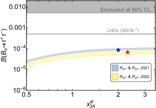
(a)

      

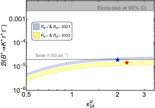
(b)

Figure 3.7: The branching fractions $\mathcal{B}\left(B_{s}\rightarrow\tau^{+}\tau^{-}\right)$ (left) and $\mathcal{B}\left(B^{+}\rightarrow K^{+}\tau^{+}\tau^{-}\right)$ (right) as a function of $x_{34}^{\psi}$, with $x_{25}^{\psi}$ varied in the range $x_{25}^{\psi}=[0.3,\,0.35]$ ($[0.4,\,0.45]$) preferred by $R_{K^{(*)}}^{2022}$ ($R_{K^{(*)}}^{2021}$), obtaining the yellow (blue) band. The rest of the parameters are fixed as in Table 5. Current exclusion limits are displayed, along with their future projections. The blue (red) star shows BP1 (BP2).

The explanation of $R_{D^{(*)}}$ in our model requires a large $U_{1}$ contribution to the 4-fermion operator $(\bar{c}_{L}\gamma_{\mu}b_{L})(\bar{\tau}_{L}\gamma^{\mu}\nu_{\tau L})$. Therefore, large contributions to the rare decays $B_{s}\rightarrow\tau\tau$ and $B\rightarrow K\tau\tau$ arise via $SU(2)_{L}$ invariance of the $U_{1}$ couplings. The respective branching fractions are of order $10^{-7}$ in the SM and mild upper bounds have been obtained by LHCb LHCb:2017myy and BaBar BaBar:2016wgb , respectively.

In Fig. 3.7, we plot the branching fractions as a function of $x_{34}^{\psi}$, while $x_{25}^{\psi}$ is varied in the ranges compatible with 2021 and 2022 $R_{K^{(*)}}$, respectively. We find that the predictions are far below the current bounds, however they lie closer to the expected future bounds from LHCb and Belle II data LHCb:2018roe ; Belle-II:2018jsg . This prediction is different in non-fermiophobic 4321 models Cornella:2019hct ; Cornella:2021sby ; Barbieri:2022ikw , where these contributions are enhanced and all the parameter space will be tested in $B^{+}\rightarrow K^{+}\tau^{+}\tau^{-}$ by Belle II.

$\boldsymbol{B\rightarrow K\nu\bar{\nu}}$

The $U_{1}$ leptoquark does not contribute at tree-level to $b\rightarrow s\nu\nu$ transitions, and the tree-level exchange of the $Z^{\prime}$ is suppressed due to the down-aligned flavour structure. However, loop-level corrections can lead to an important enhancement of the channel $B\rightarrow K\nu_{\tau}\bar{\nu}_{\tau}$ Cornella:2021sby . We parameterise corrections to the SM branching fraction as

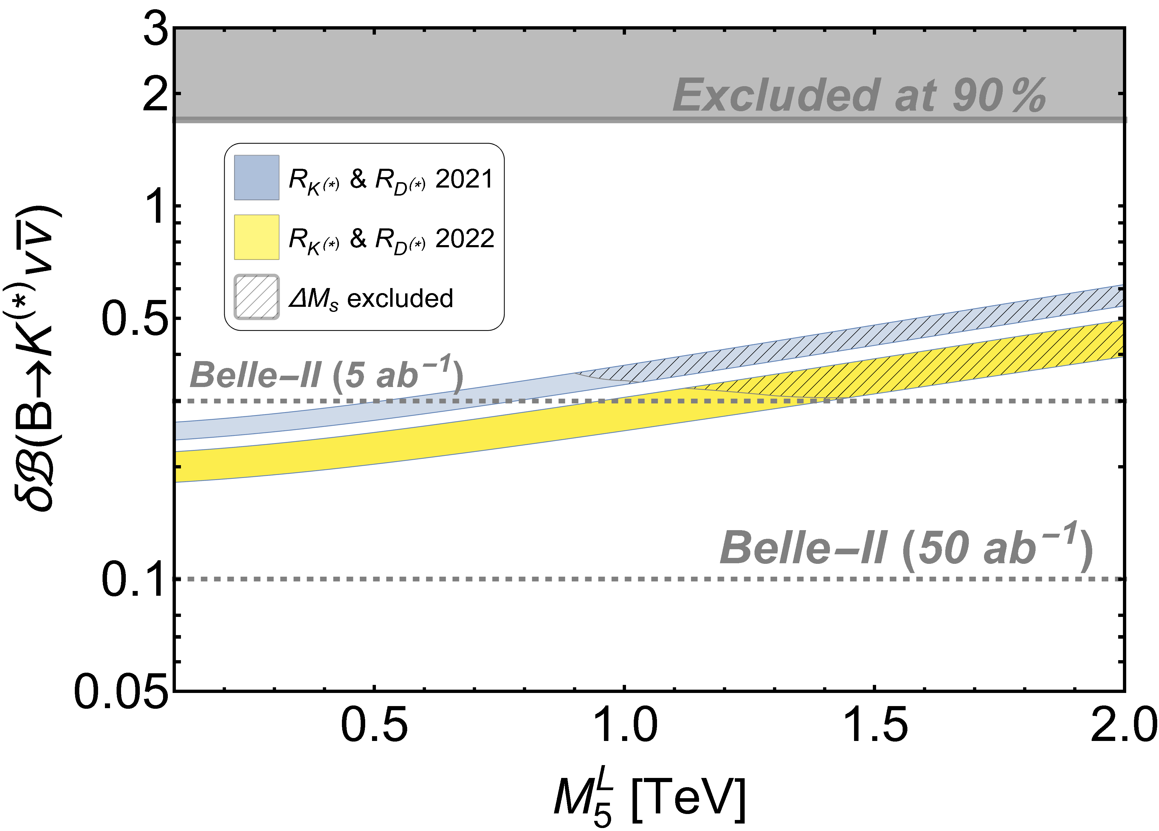
Figure 3.8: $\delta\mathcal{B}(B\rightarrow K^{(*)}\nu\bar{\nu})$ (Eq. (3.45)) as a function of the 5th family vector-like mass term. $x_{25}^{\psi}$ is varied in the range $x_{25}^{\psi}=[0.3,\,0.35]$ ($[0.4,\,0.45]$) preferred by $R_{K^{(*)}}^{2022}$ ($R_{K^{(*)}}^{2021}$ ), obtaining the yellow (blue) band. The hatched region is excluded by the $\Delta M_{s}$ bound, see Eq. (D.24). The gray region is excluded by current experimental measurements, the dashed line indicates the projected future bound.

$$\delta\mathcal{B}(B\rightarrow K^{(*)}\nu\bar{\nu})=\frac{\mathcal{B}(B\rightarrow K^{(*)}\nu\bar{\nu})}{\mathcal{B}(B\rightarrow K^{(*)}\nu\bar{\nu})_{\mathrm{SM}}}-1\approx\frac{1}{3}\left|\frac{C_{\nu\nu}^{\mathrm{NP}}+C_{\nu\nu}^{\mathrm{SM}}}{C_{\nu\nu}^{\mathrm{SM}}}\right|^{2}-\frac{1}{3}\,,$$ (3.45)

where the EFT and the Wilson coefficients are defined in Appendix D.7.

As depicted in Fig. D.3, the main contributions are a semileptonic box diagram mediated by $U_{1}$ and a triangle diagram correction to the flavour-violating $bsZ^{\prime}$ vertex, plus the RGE-induced contribution via the $U_{1}$-mediated operator $(\overline{s}_{L}\gamma_{\mu}b_{L})$ $(\overline{\tau}_{L}\gamma^{\mu}\tau_{L})$, denoted as $C_{\nu,U}^{\mathrm{RGE}}$. The former two 1-loop contributions are dominated by the fifth VL charged lepton and grow with its bare mass, $M_{5}^{L}$. This way, the overall contribution to $B\rightarrow K\nu\bar{\nu}$ can be sizable, yielding up to $\mathcal{O}(1)$ corrections with respect to the SM value, as depicted in Fig. 3.8. The details of the calculation are found in Appendix D.7.

For low $M_{5}^{L}$, the value of $\delta\mathcal{B}(B\rightarrow K^{(*)}\nu\bar{\nu})$ corresponds to $C_{\nu,U}^{\mathrm{RGE}}$. For large $M_{5}^{L}$, however, we have seen that stringent constraints from $B_{s}-\bar{B_{s}}$ meson mixing play an important role, see Section 3.4.4. This constraint is depicted as the hatched region in Fig. 3.8, correlating $B\rightarrow K\nu\bar{\nu}$ and $\Delta M_{s}$, a feature which has not been highlighted in other analyses. In particular, $\Delta M_{s}$ rules out the region where $\delta\mathcal{B}(B\rightarrow K^{(*)}\nu\bar{\nu})$ can reach values close to current experimental limits. Nevertheless, the Belle II collaboration will measure $\mathcal{B}(B\rightarrow K^{(*)}\nu\bar{\nu})$ up to 10% of the SM value Belle-II:2018jsg , hence testing all the parameter space of the model.

Our signal of $B\rightarrow K^{(*)}\nu\bar{\nu}$ also offers a great opportunity to disentangle our twin PS framework from non-fermiophobic 4321 models and the $\mathrm{PS}^{3}$ model Cornella:2019hct ; Cornella:2021sby ; Barbieri:2022ikw ; Bordone:2017bld , as they predict a much smaller signal (see Fig. 4.4 of Cornella:2021sby and compare their purple region with our Fig. 3.8).

3.4.8 Perturbativity

The explanation of the $R_{D^{(*)}}$ anomaly requires large mixing angles $s_{34}^{Q}$ and $s_{34}^{L}$, which translate into a sizeable Yukawa coupling $x_{34}^{\psi}$, thus pushing the model close to the boundary of the perturbative domain. Perturbativity is a serious constraint over our model, since we need the low-energy 4321 theory to remain perturbative until the high scale of the twin Pati-Salam symmetry. When assessing the issue of perturbativity, two conditions must be satisfied:

• Firstly, the low-energy observables must be calculable in perturbation theory. For Yukawa couplings, we consider the typical bound $x_{34}^{\psi}<\sqrt{4\pi}$. Regarding the gauge coupling $g_{4}$, standard perturbativity criteria imposes the beta function criterium Goertz:2015nkp $\left|\beta_{g_{4}}/g_{4}\right|<1$, which yields $g_{4}<4\pi\sqrt{3}/\sqrt{28}\approx 4.11$.

• Secondly, the couplings must remain perturbative up to the energy scale of the UV completion, i.e. we have to check that the couplings of the model do not face a Landau pole below the energy scale of the twin PS symmetry, namely $\mu\approx 1\,\mathrm{PeV}$.

The phenomenologically convenient choice of large $g_{4}$ is not a problem for the extrapolation in the UV, thanks to the asymptotic freedom of the $SU(4)$ gauge factor (see Fig. G.1). To investigate the running of the most problematic Yukawa $x_{34}^{\psi}$, we use the one-loop renormalisation group equations of the 4321 model (see Appendix G).

The running of the effective Yukawa couplings is protected, as the top Yukawa is order 1 and all the other are smaller, SM-like (see the discussion in Section 3.2). This feature is different from DiLuzio:2018zxy , where the top mass was accidentally suppressed by the equivalent of $c_{34}^{Q}$ in our model, hence requiring a large, non-perturbative top Yukawa to preserve the top mass. Instead, in our model the effective top Yukawa arises proportional to the maximal angle $s_{34}^{Q}$, rendering the top Yukawa natural and perturbative. The matrices of couplings $x_{Q,L}$ and $\lambda_{15}$ are defined as (assuming small $x_{35}^{\psi}$ as discussed in Section 3.4.4)

$$x_{\psi}=\left(\begin{array}[]{ccc}x_{16}^{\psi}&0&0\\ 0&x_{25}^{\psi}&0\\ 0&0&x_{34}^{\psi}\end{array}\right)\,,\quad\lambda_{15}=\left(\begin{array}[]{ccc}\lambda_{15}^{6}&0&0\\ 0&\lambda_{15}^{5}&0\\ 0&0&\lambda_{15}^{4}\end{array}\right)\,,\quad\psi=Q,\,L\,.$$ (3.46)

The Yukawas $x_{25}^{\psi}$ and $x_{16}^{\psi}$ are not dangerous as they are order 1 of smaller. The problematic Yukawa is $x_{34}^{\psi}$, which is required to be large in order to both the LFU ratios, and also it is connected with the physical mass of the fourth lepton as per Eq. (A.12). Large $\lambda_{15}^{5}$ is also required to obtain a large splitting of VL masses, which leads to a large $\theta_{LQ}$ as required by $R_{D^{(*)}}$.

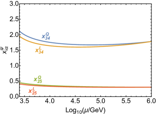
(a)

      

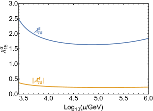
(b)

Figure 3.9: RGE of the fundamental Yukawa couplings in our benchmark scenario (Table 5) from the TeV scale to the scale of the twin Pati-Salam symmetry $\mu\sim 1\,\mathrm{PeV}$. The left panel shows the $x_{i\alpha}^{\psi}$ Yukawas which lead to the mixing between SM fermions and vector-like partners. The right panel shows the $\lambda_{15}$ Yukawas which split the vector-like masses of quarks and leptons.

Fig. 3.9 shows that the Yukawas of our benchmark scenario remain perturbative up to the high energy scale $\mu\approx 1\,\mathrm{PeV}$, thanks to the choice of a large $g_{4}=3.5$. However, we have checked that the Landau pole is hit when $x_{34}^{\psi}>2.5$, hence this region should be considered as disfavoured by perturbativity.

The small RGE effects that break the PS universality of the Yukawa couplings are below 8% in any case, hence the universality of the couplings is preserved at the TeV scale in good approximation.

3.4.9 High-$p_{T}$ signatures

General 4321 models predict a plethora of high-$p_{T}$ signatures involving the heavy gauge bosons and at least one family of vector-like fermions, requiring dedicated analyses such as those in DiLuzio:2018zxy ; Baker:2019sli ; Cornella:2021sby . In particular, our model predicts a similar high-$p_{T}$ phenomenology as that of DiLuzio:2018zxy , which also considers effective $U_{1}$ couplings via mixing with three families of vector-like fermions. However, the bounds obtained in the high-$p_{T}$ analysis of DiLuzio:2018zxy are outdated. Moreover, certain differences arise due to the underlying twin Pati-Salam symmetry in our model, plus the different implementation of the scalar sector and VEV structure. Furthermore, we anticipate that some bounds obtained in Cornella:2021sby ; Baker:2019sli might be overestimated for our model, as they usually consider large couplings to right-handed third family fermions, motivating a dedicated analysis.

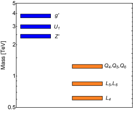
(a)

   

Particle	Decay mode	$\mathcal{B}(\mathrm{BP})$	$\Gamma/M$
$U_{1}$	$Q_{3}L_{5}+Q_{5}L_{3}$	$\sim 0.47$	0.32
	$Q_{3}L_{3}$	$\sim 0.22$
	$Q_{5}L_{5}$	$\sim 0.24$
	$Q_{i}L_{a}+Q_{a}L_{i}$	$\sim 0.07$
$g^{\prime}$	$Q_{3}Q_{3}$	$\sim 0.3$	0.5
	$Q_{5}Q_{5}$	$\sim 0.3$
	$Q_{6}Q_{6}$	$\sim 0.3$
	$Q_{1}Q_{6}$+$Q_{2}Q_{5}+Q_{3}Q_{4}$	$\sim 0.1$
$Z^{\prime}$	$L_{5}L_{5}$	$\sim 0.29$	0.24
	$L_{6}L_{6}$	$\sim 0.29$
	$L_{3}L_{3}$	$\sim 0.27$
	$Q_{3}Q_{3}$+$Q_{5}Q_{5}+Q_{6}Q_{6}$	$\sim 0.09$
	$L_{1}L_{6}+L_{2}L_{5}+L_{3}L_{4}$	$\sim 0.06$

(b)

Figure 3.10: (Left) Spectrum of new vector bosons and fermions in our benchmark scenario (BP, Table 5) around the TeV scale. (Right) Main decay channels of the new vectors $U_{1}$, $g^{\prime}$ and $Z^{\prime}$ in BP. Addition (+) implies that the depicted channels have been summed when computing the branching fraction $\mathcal{B}(\mathrm{BP})$. $i=1,2$ and $a=5,6$.

We have included the particle spectrum of our benchmark scenario in Fig. 3.10a, as a typical configuration for the masses of the new vectors and fermions. Table 3.10b shows the main decay channels of the new vector bosons, which feature large decay widths $\Gamma/M$ due to all the available decay channels to vector-like fermions, plus the choice of large $g_{4}=3.5$ close to perturbativity bounds.

In this section, we revisit some of the most simple collider signals, such as coloron dijet searches and $Z^{\prime}$ dilepton searches. We will also comment on $U_{1}$ searches, coloron ditop searches and vector-like fermions. We will point out the differences between our framework and general 4321 models, motivating a future manuscript dedicated to specific high-$p_{T}$ signals of the twin PS model.

Coloron signals

The heavy colour octet has a large impact over collider searches for 4321 models, and its production usually sets the lower bound on the scale of the model. In our case, the heavy coloron has a gauge origin, hence the coloron couplings to two gluons are absent at tree-level, reducing the coloron production at the LHC. Moreover, in the motivated scenario $\left\langle\phi_{3}\right\rangle\gg\left\langle\phi_{1}\right\rangle$, the coloron is slightly heavier than the vector leptoquark at roughly $M_{g^{\prime}}\approx\sqrt{2}M_{U_{1}}$, helping to suppress the impact of the coloron over collider searches while preserving a slightly lighter $U_{1}$ for $R_{D^{(*)}}$. In the scenario $g_{4}\gg g_{3,1}$, the coupling strength of the coloron is roughly $g_{4}$, which receives NLO corrections via the $K$-factor Fuentes-Martin:2019ign ; Fuentes-Martin:2020luw

$$K_{\mathrm{NLO}}\approx\left(1+2.65\frac{g_{4}^{2}}{16\pi^{2}}+8.92\frac{g_{s}^{2}}{16\pi^{2}}\right)^{-1/2}\,,\quad g_{g^{\prime}}\approx K_{\mathrm{NLO}}g_{4}\,.$$ (3.47)

We have computed the coloron production cross section from 13 TeV $pp$ collisions with Madgraph5 Madgraph:2014hca using the default NNPDF23LO PDF set and the coloron UFO model, publicly available in the FeynRules Feynrules:2013bka model database. We verify in Fig. 3.11a that coloron production is dominated by valence quarks, even though the coupling to left-handed bottoms is maximal. The coloron couples to light left-handed quarks (see Eq. (3.29)) via the mixing $s_{25}^{Q}\approx s_{16}^{Q}$ of $\mathcal{O}(0.1)$, which interferes destructively with the flavour-universal term, allowing for a certain cancellation of the left-handed couplings to light quarks. However, the coloron is still produced via the flavour–universal couplings to right-handed quarks.

We estimate analytically the branching fraction to all SM quarks excluding tops, and then we compute the total cross section via the narrow width approximation. Finally, we confront our results with the limits for a $q\bar{q}$-initiated spin-1 resonance provided by CMS in Fig. 10 of CMS:2019gwf . The results are displayed in Fig. 3.12a, where we have varied the coupling to light LH quarks $\kappa_{qq}$ and fixed the rest of parameters as in Table 5. We find bounds ranging from $M_{g^{\prime}}\apprge 2.5\,\mathrm{TeV}$ when $\kappa_{qq}\approx 0$ and $M_{g^{\prime}}\apprge 3\,\mathrm{TeV}$ when $\kappa_{qq}\approx g_{s}^{2}/g_{4}^{2}$. These bounds are slightly milder than those obtained in Cornella:2021sby , the reason being that in Cornella:2021sby right-handed bottom quarks are assumed to couple maximally to the coloron, while in our model this coupling is suppressed.

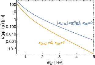
(a)

      

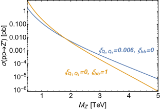
(b)

Figure 3.11: Production cross sections via 13 TeV $pp$ collisions for the coloron (left) and $Z^{\prime}$ (right), via their typical couplings to valence quarks (blue) and bottoms (orange). The choice of $\xi_{Q_{1}Q_{1}}=0.006$ corresponds to a mixing angle $s_{16}^{Q}\approx 0.2$.

We expect to find more stringent bounds in resonant coloron production with $t\bar{t}$ final states, due to the maximal couplings of the coloron to the third generation EW quark doublet. According to the recent analysis in Cornella:2021sby , our benchmark scenario would lie below current bounds, due to the large decay width $\Gamma_{g^{\prime}}/M_{g^{\prime}}\approx 0.5$ provided by extra decay channels to TeV scale vector-like quarks. The limit over the coloron mass is roughly 3.5 TeV, however this bound might be overestimated again for our model due to the different description of RH third family quarks. Reconstructing the $t\bar{t}$ channel requires a dedicated analysis and a different methodology, which is beyond the scope of this article, and we leave it for a future work.

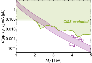
(a)

      

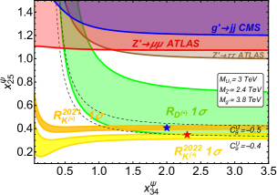
(b)

Figure 3.12: (Left) Total cross section for the coloron dijet channel in the narrow width approximation, with $\left|\kappa_{qq}\right|$ varied in the range $\left|\kappa_{qq}\right|=[0,g_{s}^{2}/g_{4}^{2}]$, where $q=Q_{1},Q_{2}$. The rest of parameters are fixed as in Table 5 for both panels. The exclusion bound from CMS is shown in green. (Right) Parameter space in the plane ($x_{34}^{\psi}$, $x_{25}^{\psi}$) compatible with the LFU ratios. The dashed lines show contours of constant $C_{9}^{U}$. The regions excluded by the collider searches considered are included. The blue (red) star shows BP1 (BP2).

$Z^{\prime}$ signals

For the $Z^{\prime}$ boson, the flavour-universal couplings to valence quarks are more heavily suppressed than those of the coloron, via the small ratio $g_{Y}^{2}/g_{4}^{2}$. Therefore, cancellation between the left-handed mixing term proportional to $s_{25}^{Q}\approx s_{16}^{Q}$ and the flavour-universal one is not possible here. In contrast with the coloron, the large LH couplings to bottoms can play a role in $Z^{\prime}$ production. The production cross section is estimated via the same methodology as for the coloron above. We do not consider any NLO corrections in this case, following the methodology of Baker:2019sli . In Fig. 3.11b we show that the production via bottoms is larger than the production via valence quarks for a light $Z^{\prime}$, however the production via valence quarks is bigger for $M_{Z^{\prime}}\apprge 2\,\mathrm{TeV}$, and shall not be neglected as it commonly happens in the literature (see e.g. Baker:2019sli ).

We estimate the branching fraction to muons and taus, and we compute the total decay width via the narrow width approximation. We confront our results with the limits from the dilepton resonance searches by ATLAS, Fig. 4 of ATLAS:2017fih for muons and Fig. 7 (c) of ATLAS:2017eiz for taus. We display the results in Figs. 3.13a and 3.13b. In Fig. 3.12b we see that these processes, along with coloron dijet searches, mildly constrain the region of large $x_{25}^{\psi}$. Ditau searches are more competitive than dimuon searches or coloron dijet searches, due to the branching fractions to muons and light quarks being suppressed by mixing angles $s_{25}^{Q,L}\sim\mathcal{O}(0.1)$. Instead, the ditau channel is enhanced by maximal 3-4 mixing, and sets bounds of roughly $M_{Z^{\prime}}>1.5\,\mathrm{TeV}$, see Fig. 3.13b.

$U_{1}$ signals

Leptoquark pair-production cross sections at the LHC are dominated by QCD dynamics, and thus are largely independent of the leptoquark couplings to fermions. Therefore, we are able to safely compare with the analyses of Refs. Cornella:2021sby ; Baker:2019sli . A certain model dependence is present in the form of non-minimal couplings to gluons, however these couplings are absent in models where $U_{1}$ has a gauge origin. According to Fig. 3.3 of Cornella:2021sby , current bounds over direct production exclude $M_{U_{1}}<1.7\,\mathrm{TeV}$, and the future bound is expected to exclude $M_{U_{1}}<2.1\,\mathrm{TeV}$ if no NP signal is found during the high-luminosity phase of the LHC.

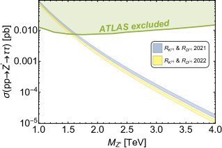
(a)

      

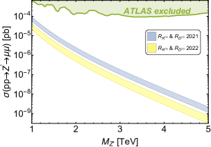
(b)

Figure 3.13: Total cross section for ditau (left) and dimuon (right) production via a heavy $Z^{\prime}$ in the narrow width approximation, with $x_{25}^{\psi}$ varied in the range $x_{25}^{\psi}=[0.3,\,0.35]$ ($[0.4,\,0.45]$) preferred by $R_{K^{(*)}}^{2022}$ ($R_{K^{(*)}}^{2021}$ ), obtaining the yellow (blue) band. The exclusion bounds from ATLAS are shown in green.

An important constraint over $U_{1}$ arises from modifications of the high-$p_{T}$ tail in the dilepton invariance mass distribution of the Drell-Yan process $pp\rightarrow\tau^{+}\tau^{-}+X$, induced by $t$-channel $U_{1}$ exchange Diaz:2017lit ; Baker:2019sli ; Angelescu:2021lln ; Cornella:2021sby . This channel is well motivated by the $U_{1}$ explanation of $R_{D^{(*)}}$, which unavoidably predicts a large $b\tau U_{1}$ coupling. The scenario $\beta_{b\tau}^{R}=0$ considered in the study of Baker:2019sli ; Cornella:2021sby fits well the twin Pati-Salam framework, up to a re-scaling of the $U_{1}$ coupling strength as $g_{U}\rightarrow g_{U}\beta_{b\tau}^{L}$, in order to account for the fact that our $\beta_{b\tau}^{L}$ is not maximal but $\beta_{b\tau}^{L}\approx c_{\theta_{LQ}}\approx 0.67$ in our benchmark scenario, where we obtain $g_{U}\approx 2.3$. According to the left panel of Fig. 3.3 in Cornella:2021sby , the 3 TeV leptoquark of our benchmark lies well below the current bounds, but within projected limits for the high luminosity phase of LHC. Finding $U_{1}$ much below 3 TeV enters in tension with $pp\rightarrow g^{\prime}\rightarrow t\bar{t}$ as explained before, due to the approximate relation $M_{g^{\prime}}\approx\sqrt{2}M_{U_{1}}$ that entangles the masses of $U_{1}$ and the coloron (although the bound is probably overestimated for our dominantly left-handed model).

The twin Pati-Salam model could provide a good $U_{1}$ candidate for the 3$\sigma$ excess at CMS CMS-PAS-EXO-19-016 pointing to a 2 TeV $U_{1}$ leptoquark in the well motivated channel $pp\rightarrow U_{1}\rightarrow\tau\tau$, once the extra decay channels to vector-like fermions are considered, assuming that the bound from $pp\rightarrow g^{\prime}\rightarrow t\bar{t}$ is indeed overestimated.

Vector-like fermions

The presence of vector-like fermions is of fundamental importance to discriminate between the different implementations of the 4321 model addressing the $B$-anomalies. A common constraint arises from $\Delta F=2$ transitions at low energies, which require that the vector-like charged lepton that mixes with muons is light (see Fig. 3.3a). The natural mass of the quark partner of $L_{5}$ should not lie far away due to the approximate Pati-Salam universality, the small breaking effects given by the VEV $\left\langle\Omega_{15}\right\rangle$. In particular, in our benchmark scenario we obtained $M_{5}^{L}\approx 0.8\,\mathrm{TeV}$ and $M_{5}^{Q}\approx 1.2\,\mathrm{TeV}$. The flavour structure of the model naturally predicts that both $Q_{5}$ and $L_{5}$ are strongly coupled to the third generation of SM fermions.

The twin Pati-Salam model features also $L_{4}$ and $Q_{4}$ as a relevant pair of vector-like fermions, which mix maximally with the third generation in order to obtain the large couplings required for $R_{D^{(*)}}$, and also to fit the top mass without perturbativity issues. This implies that their bare mass terms in the original Lagrangian are small, therefore their physical masses are dominated by $x_{34}^{\psi}\left\langle\phi_{3,1}\right\rangle$, see Eq. (A.6) and (A.12). In the motivated scenario $\left\langle\phi_{3}\right\rangle\gg\left\langle\phi_{1}\right\rangle$ which slightly suppresses the production of the coloron, we found $L_{4}$ to be very light, featuring roughly 600 GeV in our benchmark. Instead, $Q_{4}$ can lie above 1 TeV, featuring roughly 1.2 TeV in our benchmark. The couplings of $L_{4}$ to SM fermions are smaller than those of $L_{5}$, but it is dominantly coupled to third generation fermions.

Interestingly, CMS recently performed a search for the vector-like leptons of the 4321 model CMS:2022cpe , finding 2.8$\sigma$ preference for a vector-like lepton with 600 GeV, however the analysis assumes EW production only and maximal couplings to the third generation. If $Z^{\prime}$-assisted production is included, $L_{5}$ a with mass at 800 GeV could be a good candidate for the anomaly. Furthermore, $L_{4}$ at 600 GeV could also provide a good fit once not maximal couplings are considered, however this requires verification in a future dedicated analysis. Non-fermiophobic 4321 models, such as Cornella:2019hct ; Cornella:2021sby , predict a heavier vector-like lepton, while DiLuzio:2018zxy also predicts $L_{5}$ at around 800 GeV but a heavier $L_{4}$. Regarding the sixth vector-like fermions $L_{6}$ and $Q_{6}$, we expect them to have similar masses as $L_{5}$ and $Q_{5}$ in order to preserve the GIM-like suppression of 1-2 FCNCs, they are feebly coupled to first generation fermions but not to the second or third generation.

Current bounds on vector-like quarks lie around 1 TeV, however they are usually very model dependent. Our vector-like quarks are pair produced through gluon fusion and through the decay of the coloron, which is very likely to be kinematically allowed. Their decays leave a large amount of third generation fermions in the final state, following a similar mechanism as the one discussed in DiLuzio:2018zxy . The twin Pati-Salam model naturally predicts light vector-like quarks with masses around 1 TeV, which is a feature not present in all other 4321 models and could motivate specific searches.

4 Comparison with other models

Table 4 includes a simplified set of observables that allows to disentangle the twin PS model from the ones that are already in the market. A further discussion can be found in the two following sections.

4.1 Non-fermiophobic 4321 models (including the $\mathrm{PS}^{3}$ model)

The twin PS model is built as a fermiophobic framework, where all chiral fermions are singlets under the TeV scale $SU(4)$. This is a crucial difference between our model and the non-fermiophobic 4321 models Cornella:2019hct ; Cornella:2021sby ; Barbieri:2022ikw ; Fuentes-Martin:2020bnh ; Fuentes-Martin:2020hvc and its UV completions (including the $\mathrm{PS}^{3}$ model Bordone:2017bld ), where the third family of chiral fermions transforms under the TeV scale $SU(4)$. This implies large left- and right-handed third family couplings to $SU(4)$ gauge bosons. By contrast, in our theory of flavour, the right-handed couplings of SM fermions to $U_{1}$ (and also to $Z^{\prime}$ and $g^{\prime}$) arise via small mixing angles connected to the origin of second family fermion masses, hence the twin PS model predicts dominantly left-handed $U_{1}$ couplings. The low-energy phenomenology between both approaches is radically different.

	twin PS	fermiophobic 4321	$\mathrm{PS}^{3}$	non-fermiophobic 4321
Refs.	this paper	DiLuzio:2017vat ; DiLuzio:2018zxy	Bordone:2017bld ; Bordone:2018nbg	Cornella:2019hct ; Cornella:2021sby ; Barbieri:2022ikw ; Greljo:2018tuh
Theory of flavour	Yes	No	Yes	No
$R_{D^{(*)}}$	$\Delta R_{D}=\Delta R_{D^{*}}$	$\Delta R_{D}=\Delta R_{D^{*}}$	$\Delta R_{D}>\Delta R_{D^{*}}$	$\Delta R_{D}>\Delta R_{D^{*}}$
$\mathcal{B}\left(\tau\rightarrow 3\mu\right)$	$10^{-8}$	$\lesssim 10^{-11}$	$10^{-9}$	-
$\mathcal{B}\left(\tau\rightarrow\mu\gamma\right)$	$10^{-9}$	$\lesssim 10^{-11}$	$10^{-8}$	$10^{-8}$
$\mathcal{B}\left(\tau\rightarrow\mu\phi\right)$	$10^{-9}$	$10^{-11}$	$10^{-10}$	$10^{-10}$
$\mathcal{B}\left(B_{s}\rightarrow\tau\mu\right)$	$10^{-6}$	$10^{-7}$	$10^{-5}$	$10^{-5}$
$\mathcal{B}\left(B_{s}\rightarrow\tau\tau\right)$	$10^{-4}$	-	$10^{-3}$	$10^{-3}$
$\mathcal{B}\left(B\rightarrow K\tau\tau\right)$	$10^{-5}$	-	$10^{-4}$	$10^{-4}$
$\delta\mathcal{B}(B\rightarrow K^{(*)}\nu\bar{\nu})$ (3.45)	$0.3$	-	$0.2$	$0.2$
VL fermion families	3	3	1	1
High-$p_{T}$ constraints	Mild	Mild	Tight	Tight

Table 4: Main observables to distinguish the twin PS model from other proposals. The numbers are only indicative, as these predictions may vary along the parameter space of the different models. The dash (-) indicates that the observable was not considered or numbers were not given in the corresponding references. In the high-$p_{T}$ row we broadly refer to how constrained is the model by high-$p_{T}$ searches.

In terms of the charged current anomalies $R_{D^{(*)}}$, the twin PS model only predicts the effective operator $(\bar{c}_{L}\gamma_{\mu}b_{L})(\bar{\text{$\tau$}}_{L}\gamma^{\mu}\nu_{\tau L})$, and hence both $R_{D}$ and $R_{D^{*}}$ are corrected in the same direction and with the same size. Instead, non-fermiophobic 4321 models also predict the scalar operator $(\bar{c}_{L}b_{R})(\bar{\text{$\tau$}}_{R}\nu_{\tau L})$. Due to the presence of this operator, the effect on $\Delta R_{D}$ is larger than on $\Delta R_{D^{*}}$ (about 5/2 larger for the $\mathrm{PS}^{3}$ model, see Eq. (27) in Bordone:2017bld ).

Another key observable is $B\rightarrow K\nu\nu$, for which the twin PS model predicts a larger branching fraction that will be fully tested by Belle II. Instead, non-fermiophobic 4321 models predict a smaller branching fraction, see Fig. 4.4 of Cornella:2021sby and compare their purple region with our Fig. 3.8. Moreover, in our analysis of $B\rightarrow K\nu\nu$ we have highlighted correlations with $B_{s}-\bar{B}_{s}$ mixing due to the loops being dominated by the same VL charged lepton, a feature which is missing in the analysis of Cornella:2021sby .

Regarding the rest of the observables, broadly speaking the twin PS model predicts larger branching fractions for LFV processes. The exception is $\tau\rightarrow\mu\gamma$, which is enhanced in non-fermiophobic models via a chirality flip with the bottom quark running in the loop. The rare decays $B_{s}\rightarrow\tau\tau$ and $B\rightarrow K\tau\tau$ are larger in non-fermiophobic models due to the presence of scalar operators connected to the third family RH couplings. The LHCb and Belle II collaborations will test regions of the parameter space and allow to disentangle between the different 4321 approaches.

High-$p_{T}$ searches also offer a window to disentangle both approaches, since most of the constraints afflicting non-fermiophobic 4321 scenarios are relaxed in the dominantly left-handed scenario of the twin PS model. Particularly relevant are also the different implementations of vector-like fermions.

Regarding the $\mathrm{PS}^{3}$ model, it predicts the same signals as non-fermiophobic 4321 models plus enhanced LFV. It can be disentangled from the twin PS model via the set of observables already discussed.

4.2 Fermiophobic 4321 models

Up to our knowledge, the only fermiophobic 4321 model proposed in the literature is that of Ref. DiLuzio:2017vat , whose phenomenology was studied in detail in DiLuzio:2018zxy . This model presents a simplified fermiophobic scenario with a rather assumed flavour structure motivated by the phenomenology, including an ad-hoc alignment of SM-like Yukawas and VL-chiral fermion mixing. Furthermore, DiLuzio:2017vat does not address the question of quark and lepton masses (is not a theory of flavour), unlike the model proposed here. It lacks from quark-lepton unification of SM fermions and leads to a less predictive framework than the twin PS model.

The twin Pati-Salam model leads to an effective fermiophobic 4321 model. However, the underlying twin PS symmetry implies universality of key parameters, leading to extra constraints and correlations between observables, which are not present in the analyses of DiLuzio:2017vat ; DiLuzio:2018zxy . For example, $R_{D^{(*)}}$ and $R_{K^{(*)}}$ are correlated here due to the universality of $x_{25}^{\psi}$ and $x_{34}^{\psi}$, leading to quasi-universal mixing angles $s_{25}^{Q,L}$ and $s_{34}^{Q,L}$. By contrast, such mixing angles are free parameters in DiLuzio:2017vat ; DiLuzio:2018zxy and one can explain $R_{D^{(*)}}$ without giving any contribution to $R_{K^{(*)}}$. As a consequence, it was required a dedicated analysis to show that $R_{D^{(*)}}$ can be explained in the twin PS model while being compatible with the recent data on $R_{K^{(*)}}$, as we did in this paper.

Since the twin PS model is a theory of flavour, while DiLuzio:2017vat ; DiLuzio:2018zxy is not, new signals are predicted in LFV processes connected to the origin of fermion masses and mixings. The twin PS model predicts non-vanishing $\mu-\tau$ mixing, leading to striking signals in $\tau\rightarrow 3\mu$ and $\tau\rightarrow\mu\gamma$ close to current experimental bounds, summarised in our Figs. 3.4a and 3.4b. The large contributions to the branching fractions of $\tau\rightarrow 3\mu$ and $\tau\rightarrow\mu\gamma$ are mediated by the $Z^{\prime}$ boson, see the purple region in Figs. 3.4a and 3.4b. On the other hand, in general fermiophobic 4321 models DiLuzio:2017vat ; DiLuzio:2018zxy only a much smaller 1-loop $U_{1}$ mediated signal is predicted. This signal was not computed in Refs. DiLuzio:2017vat ; DiLuzio:2018zxy as it is very small compared to the experimental bounds, but we have computed it here for the sake of comparison, and it is depicted as the blue region in Figs. 3.4a and 3.4b. In a similar way, we obtain $\mathcal{B}(\tau\rightarrow\mu\phi)$ two orders of magnitude larger than in DiLuzio:2017vat ; DiLuzio:2018zxy .

Finally, the fermion mixing predicted by the twin PS model avoids current constraints coming from CKM unitarity, $\Delta F=2$ and EW precision observables presented in Fajfer:2013wca . The reasons are the absence of SM-like Yukawa couplings for chiral fermions in the original basis (as they will be generated indeed via this mixing), along with the fact that VL quark EW doublets and SM quark EW singlets do not mix, hence the VL quark doublet remains unsplitted. Remarkably, this is different from DiLuzio:2017vat ; DiLuzio:2018zxy , where mixing between the SM quark singlets and the VL (right-handed) quark doublet was induced due to the presence of the SM-like Yukawa couplings for chiral fermions, leading to possible splitting of the VL quark doublet, which constrains the mixing angles for third generation quarks according to the analysis in Fajfer:2013wca .

5 Conclusions

We have performed a comprehensive phenomenological analysis of the twin Pati-Salam model, which is capable of explaining anomalies in LFU ratios of $B$-decays, while simultaneously accounting for the fermion masses and mixings of the SM. The basic idea of this model is that all three families of SM chiral fermions transform under one PS group, while families of vector-like fermions transform under the other one. Vector leptoquark couplings and SM Yukawa couplings emerge together after mixing of the chiral fermions with the vector-like fermions, thereby providing a direct link between $B$-physics and fermion masses and mixings. The model was originally built to explain the 2021 picture of LFU anomalies in the $R_{K^{(*)}}$ and $R_{D^{(*)}}$ ratios. In this updated version we have included an extended analysis considering the new 2022 LHCb data on $R_{K^{(*)}}$, which has shifted the preferred parameter space with respect to the 2021 case. The model can still explain the $R_{D^{(*)}}$ anomalies at 1$\sigma$ in a narrow window while being compatible with all data, however we expect small deviations from the SM on the $R_{K^{(*)}}$ ratios, to be tested in the future via more precise measurements of LFU by the LHCb collaboration. We also predict $\Delta R_{D}=\Delta R_{D^{*}}$, with future measurements shifting the world averages to slightly smaller central values.

Firstly, we presented a simplified version of the model that is able to explain second and third family charged fermion masses and mixings via effective Yukawa couplings, which arise naturally from mixing effects with a fourth vector-like family of fermions. However, with only a single vector-like family the model is unable to explain the $B$-anomalies in a natural way, as it does not achieve the flavour structure required by 4321 models, and hence is over constrained by flavour-violating processes such as $B_{s}-\bar{B}_{s}$ meson mixing. The latter are mediated by a heavy colour octet and a $Z^{\prime}$ that also acquire flavour-violating couplings with chiral fermions.

We then extended the simplified model to include three vector-like families, together with a $Z_{4}$ discrete symmetry to control the flavour structure. This version of the model allows for larger flavour-violating and dominantly left-handed $U_{1}$ couplings as required to address $R_{D^{(*)}}$, thanks to mixing between a fourth and fifth vector-like families which also mix with the second and third generations of SM fermions. A sixth vector-like family is included to mix with the first SM generation, for the sake of suppressing any FCNCs involving first and second generation fermions. The mechanism resembles the GIM suppression of FCNCs in the SM, featuring a similar Cabbibo-like matrix which is present in leptoquark currents, but not in neutral currents mediated by the coloron and $Z^{\prime}$.

As in the simplified twin Pati-Salam model, the origin of second and third generation charged fermion masses and mixings remains addressed via effective Yukawa couplings, featuring now a down-aligned flavour structure in the 2-3 sector (requiring a mild tuning as described in the main text) that protects from the dangerous tree-level contributions to $B_{s}-\bar{B}_{s}$ meson mixing. Non-zero 2-3 mixing in the charged lepton sector is also predicted, leading to interesting signals in $\tau\rightarrow 3\mu$ and $\tau\rightarrow\mu\gamma$, mostly due to $Z^{\prime}$ exchange, which are close to present experimental bounds in some region of the parameter space. Signals in LFV semileptonic processes mediated by $U_{1}$ at tree-level are found to lie well below current experimental limits, with the exception of $K_{L}\rightarrow e\mu$ which constrains a small region of the parameter space. However, this tension can be alleviated if the first family $U_{1}$ coupling is diluted via mixing with vector-like fermions. Tests of LFU in tau decays set important bounds over the mass of $U_{1}$ depending on its coupling to third generation fermions. Contributions of $U_{1}$ to the rare decays $B_{s}\rightarrow\tau\tau$ and $B\rightarrow K\tau\tau$ are broadly below current and projected experimental sensitivity. Instead, the rare decay $B\rightarrow K^{(*)}\nu\bar{\nu}$ offers the opportunity to fully test the model in the near future, since Belle II is expected to cover all the parameter space compatible with the LFU ratios. Remarkably, the model can be easily disentangled from all other proposals via the previous set of observables, as discussed in Section 4.

Apart from the above low-energy predictions at LHCb and Belle II, the model is also testable via high-$p_{T}$ searches at the LHC. The study of the 1-loop contribution of vector leptoquark $U_{1}$ exchange to $B_{s}-\bar{B}_{s}$ mixing revealed that the fifth vector-like lepton has to be light, around 1-2 TeV, to be compatible with the stringent bound from $\Delta M_{s}$. This is easily achieved in the twin Pati-Salam model, where light vector-like fermions are well motivated in order to naturally obtain the large mixing to fit the $R_{D^{(*)}}$ anomaly, and also to fit the heavy top mass without perturbativity issues. In particular, the fourth and fifth charged leptons are suggested as good candidates to explain the CMS excess CMS:2022cpe , but further study is required in this direction. Vector-like quarks are found to lie not far above 1 TeV in the suggested benchmark, hence motivating specific searches at LHC to be performed. Regarding the heavy vectors, dijet searches and dilepton searches set mild bounds over the mass of the coloron and $Z^{\prime}$, respectively. The more stringent bound over the scale of the model arises from the ditop searches in Baker:2019sli ; Cornella:2021sby , which push the mass of the coloron to lie above 3.5 TeV, however those bounds could be slightly overestimated for our model as they only consider non-fermiophobic 4321 scenarios. Finally, the mass range for $U_{1}$ is compatible with current bounds, and mostly lie within the projected sensitivity of the high luminosity phase of LHC. A good fit for the $3\sigma$ CMS excess in $U_{1}$ searches CMS-PAS-EXO-19-016 could be provided if the extra decay channels to vector-like fermions, assuming that the bound from ditop searches is indeed overestimated, motivating a future dedicated collider analysis.

The model proposed here features clear connections between the SM fermion masses and the leptoquark couplings which can address anomalies in LFU ratios, along with Pati-Salam universality of most of the parameters, leading to a very predictive and testable framework. The masses and mixings of first family fermion can arise along the lines of the original twin Pati-Salam model King:2021jeo , involving a new family of vector-like fermions which does not couple to $U_{1}$. Thanks to the GIM-like mechanism implemented, the phenomenology discussed in this paper would remain unaltered. However, the GIM-like mechanism introduced is accidental, and enforcing this mechanism via extra symmetries would involve the first family. Therefore, we leave the origin of first family masses, neutrino masses and the symmetry behind the GIM-like mechanism for a future manuscript, as they are uncorrelated to $B$-physics and the phenomenology discussed here.

Appendix A Mixing angle formalism

The mixing between third family and fourth family fermions arises from the following terms in the mass Lagrangian King:2020mau ,

$$\mathcal{L}_{\mathrm{mass}}\supset x_{34}^{\psi}\phi\psi_{3}\overline{\psi}_{4}+M_{4}^{\psi}\psi_{4}\overline{\psi}_{4}+\mathrm{h.c.}$$ (A.1)

After the scalar $\phi$ develops a VEV, we obtain

$$x_{34}^{\psi}\left\langle\phi\right\rangle\psi_{3}\overline{\psi}_{4}+M_{4}^{\psi}\psi_{4}\overline{\psi}_{4}=\left(x_{34}^{\psi}\left\langle\phi\right\rangle\psi_{3}+M_{4}^{\psi}\psi_{4}\right)\overline{\psi}_{4}=\tilde{M}_{4}^{\psi}\frac{x_{34}^{\psi}\left\langle\phi\right\rangle\psi_{3}+M_{4}^{\psi}\psi_{4}}{\sqrt{\left(x_{34}^{\psi}\left\langle\phi\right\rangle\right)^{2}+\left(M_{4}^{\psi}\right)^{2}}}\overline{\psi}_{4}\,,$$ (A.2)

where we have defined

$$\tilde{M}_{4}^{\psi}=\sqrt{\left(x_{34}^{\psi}\left\langle\phi\right\rangle\right)^{2}+\left(M_{4}^{\psi}\right)^{2}}$$ (A.3)

as the physical mass of the vector-like fermion. We can identify the mixing angles as

$$s_{34}^{\psi}=\frac{x_{34}^{\psi}\left\langle\phi\right\rangle}{\sqrt{\left(x_{34}^{\psi}\left\langle\phi\right\rangle\right)^{2}+\left(M_{4}^{\psi}\right)^{2}}}\,,\quad c_{34}^{\psi}=\frac{M_{4}^{\psi}}{\sqrt{\left(x_{34}^{\psi}\left\langle\phi\right\rangle\right)^{2}+\left(M_{4}^{\psi}\right)^{2}}}\,.$$ (A.4)

This way, the mass eigenstates are given by

$$\tilde{\psi}_{4}\equiv c_{34}^{\psi}\psi_{4}+s_{34}^{\psi}\psi_{3}\,,\qquad\tilde{\psi}_{3}\equiv c_{34}^{\psi}\psi_{4}-s_{34}^{\psi}\psi_{3}\,.$$ (A.5)

We can follow the same procedure to obtain all the mixing angles and physical masses of vector-like fermions,

$$s_{34}^{Q}=\frac{x_{34}^{\psi}\left\langle\phi_{3}\right\rangle}{\sqrt{\left(x_{34}^{\psi}\left\langle\phi_{3}\right\rangle\right)^{2}+\left(M_{4}^{Q}\right)^{2}}}\,, s_{34}^{L}=\frac{x_{34}^{\psi}\left\langle\phi_{1}\right\rangle}{\sqrt{\left(x_{34}^{\psi}\left\langle\phi_{1}\right\rangle\right)^{2}+\left(M_{4}^{L}\right)^{2}}}\,,$$ (A.6)

$$s_{25}^{Q}=\frac{x_{25}^{\psi}\left\langle\phi_{3}\right\rangle}{\sqrt{\left(x_{25}^{\psi}\left\langle\phi_{3}\right\rangle\right)^{2}+\left(M_{5}^{Q}\right)^{2}}}\,, s_{25}^{L}=\frac{x_{25}^{\psi}\left\langle\phi_{1}\right\rangle}{\sqrt{\left(x_{25}^{\psi}\left\langle\phi_{1}\right\rangle\right)^{2}+\left(M_{5}^{L}\right)^{2}}}\,,$$ (A.7)

$$s_{35}^{Q}=\frac{c_{34}^{Q}x_{35}^{\psi}\left\langle\phi_{3}\right\rangle}{\sqrt{\left(c_{34}^{Q}x_{35}^{\psi}\left\langle\phi_{3}\right\rangle\right)^{2}+\left(x_{25}^{\psi}\left\langle\phi_{3}\right\rangle\right)^{2}+\left(M_{5}^{Q}\right)^{2}}}, s_{35}^{L}=\frac{c_{34}^{L}x_{35}^{\psi}\left\langle\phi_{1}\right\rangle}{\sqrt{\left(c_{34}^{L}x_{35}^{\psi}\left\langle\phi_{1}\right\rangle\right)^{2}+\left(x_{25}^{\psi}\left\langle\phi_{1}\right\rangle\right)^{2}+\left(M_{5}^{L}\right)^{2}}}\,,$$ (A.8)

$$s_{16}^{Q}=\frac{x_{16}^{\psi}\left\langle\phi_{3}\right\rangle}{\sqrt{\left(x_{16}^{\psi}\left\langle\phi_{3}\right\rangle\right)^{2}+\left(M_{6}^{Q}\right)^{2}}}\,, s_{16}^{L}=\frac{x_{16}^{\psi}\left\langle\phi_{1}\right\rangle}{\sqrt{\left(x_{16}^{\psi}\left\langle\phi_{1}\right\rangle\right)^{2}+\left(M_{6}^{L}\right)^{2}}}\,,$$ (A.9)

$$s_{24}^{q^{c}}=\frac{x_{42}^{\psi^{c}}\langle\overline{\phi_{3}}\rangle}{\sqrt{\left(x_{42}^{\psi^{c}}\langle\overline{\phi_{3}}\rangle\right)^{2}+\left(M_{4}^{\psi^{c}}\right)^{2}}}\,, s_{24}^{e^{c}}=\frac{x_{42}^{\psi^{c}}\langle\overline{\phi_{1}}\rangle}{\sqrt{\left(x_{42}^{\psi^{c}}\langle\overline{\phi_{1}}\rangle\right)^{2}+\left(M_{4}^{\psi^{c}}\right)^{2}}}\,,$$ (A.10)

$$s_{34}^{q^{c}}=\frac{x_{43}^{\psi^{c}}\langle\overline{\phi_{3}}\rangle}{\sqrt{\left(x_{42}^{\psi^{c}}\langle\overline{\phi_{3}}\rangle\right)^{2}+\left(x_{43}^{\psi^{c}}\langle\overline{\phi_{3}}\rangle\right)^{2}+\left(M_{4}^{\psi^{c}}\right)^{2}}}\,, s_{34}^{e^{c}}=\frac{x_{43}^{\psi^{c}}\langle\overline{\phi}_{1}\rangle}{\sqrt{\left(x_{42}^{\psi^{c}}\langle\overline{\phi_{1}}\rangle\right)^{2}+\left(x_{43}^{\psi^{c}}\langle\overline{\phi_{1}}\rangle\right)^{2}+\left(M_{4}^{\psi^{c}}\right)^{2}}}\,,$$ (A.11)

$$\tilde{M}_{4}^{Q}=\sqrt{\left(x_{34}^{\psi}\left\langle\phi_{3}\right\rangle\right)^{2}+\left(M_{4}^{Q}\right)^{2}}\,, \tilde{M}_{4}^{L}=\sqrt{\left(x_{34}^{\psi}\left\langle\phi_{1}\right\rangle\right)^{2}+\left(M_{4}^{L}\right)^{2}}\,,$$ (A.12)

$$\tilde{M}_{5}^{Q}=\sqrt{\left(x_{25}^{\psi}\left\langle\phi_{3}\right\rangle\right)^{2}+\left(x_{35}^{\psi}\left\langle\phi_{3}\right\rangle\right)^{2}+\left(M_{5}^{Q}\right)^{2}}\,, \tilde{M}_{5}^{L}=\sqrt{\left(x_{25}^{\psi}\left\langle\phi_{1}\right\rangle\right)^{2}+\left(x_{35}^{\psi}\left\langle\phi_{1}\right\rangle\right)^{2}+\left(M_{5}^{L}\right)^{2}}\,,$$ (A.13)

$$\tilde{M}_{6}^{Q}=\sqrt{\left(x_{16}^{\psi}\left\langle\phi_{3}\right\rangle\right)^{2}+\left(M_{6}^{Q}\right)^{2}}\,, \tilde{M}_{6}^{L}=\sqrt{\left(x_{16}^{\psi}\left\langle\phi_{1}\right\rangle\right)^{2}+\left(M_{6}^{L}\right)^{2}}\,,$$ (A.14)

$$\widetilde{M}_{4}^{q^{c}}=\sqrt{\left(x_{42}^{\psi^{c}}\langle\overline{\phi_{3}}\rangle\right)^{2}+\left(x_{43}^{\psi^{c}}\langle\overline{\phi_{3}}\rangle\right)^{2}+\left(M_{4}^{\psi^{c}}\right)^{2}}\,, \widetilde{M}_{4}^{e^{c}}=\sqrt{\left(x_{42}^{\psi^{c}}\langle\overline{\phi_{1}}\rangle\right)^{2}+\left(x_{43}^{\psi^{c}}\langle\overline{\phi_{1}}\rangle\right)^{2}+\left(M_{4}^{\psi^{c}}\right)^{2}}\,.$$ (A.15)

Appendix B Vector-fermion interactions

B.1 Simplified model

For the $U_{1}$ couplings, in the basis of mass eigenstates we obtain

$$\frac{g_{4}}{\sqrt{2}}\hat{u}_{i}^{\dagger}\gamma^{\mu}\left(\begin{array}[]{ccc}0&0&0\\ 0&0&s_{34}^{Q}s_{34}^{L}s_{23}^{u}\\ 0&0&s_{34}^{Q}s_{34}^{L}c_{23}^{u}\end{array}\right)\hat{\nu}{}_{j}U_{1\mu}+\mathrm{h.c.}\,,\quad\frac{g_{4}}{\sqrt{2}}\hat{d}_{i}^{\dagger}\gamma^{\mu}\left(\begin{array}[]{ccc}0&0&0\\ 0&s_{34}^{Q}s_{34}^{L}s_{23}^{d}s_{23}^{e}&s_{34}^{Q}s_{34}^{L}s_{23}^{d}c_{23}^{e}\\ 0&s_{34}^{Q}s_{34}^{L}c_{23}^{d}s_{23}^{e}&s_{34}^{Q}s_{34}^{L}c_{23}^{d}c_{23}^{e}\end{array}\right)\hat{e}_{j}U_{1\mu}+\mathrm{h.c.}$$ (B.1)

For the coloron couplings, in the basis of mass eigenstates we obtain

$$\mathcal{L}_{g^{\prime}}^{\mathrm{gauge}}=\frac{g_{4}g_{s}}{g_{3}}\hat{d}_{i}^{\dagger}\gamma^{\mu}T^{a}\left(\begin{array}[]{ccc}-\frac{g_{3}^{2}}{g_{4}^{2}}&0&0\\ 0&-\left(c_{23}^{d}\right)^{2}\frac{g_{3}^{2}}{g_{4}^{2}}+\left(s_{34}^{Q}s_{23}^{d}\right)^{2}&\left(s_{34}^{Q}\right)^{2}s_{23}^{d}c_{23}^{d}\\ 0&\left(s_{34}^{Q}\right)^{2}s_{23}^{d}c_{23}^{d}&\left(s_{34}^{Q}c_{23}^{d}\right)^{2}-\left(c_{34}^{Q}c_{23}^{d}\right)^{2}\frac{g_{3}^{2}}{g_{4}^{2}}\end{array}\right)\hat{d}_{j}g_{\mu}^{a^{\prime}}+\left(d\rightarrow u\right)\,,$$ (B.2)

and for the $Z^{\prime}$

$$\mathcal{L}_{Z^{\prime},q}^{\mathrm{gauge}}=\frac{\sqrt{3}}{\sqrt{2}}\frac{g_{4}g_{Y}}{g_{1}}\hat{d}_{i}^{\dagger}\gamma^{\mu}\left(\begin{array}[]{ccc}-\frac{g_{1}^{2}}{9g_{4}^{2}}&0&0\\ 0&-\left(c_{23}^{d}\right)^{2}\frac{g_{1}^{2}}{9g_{4}^{2}}+\frac{1}{6}\left(s_{34}^{Q}s_{23}^{d}\right)^{2}&\frac{1}{6}\left(s_{34}^{Q}\right)^{2}s_{23}^{d}c_{23}^{d}\\ 0&\frac{1}{6}\left(s_{34}^{Q}\right)^{2}s_{23}^{d}c_{23}^{d}&\frac{1}{6}\left(s_{34}^{Q}c_{23}^{d}\right)^{2}-\left(c_{34}^{Q}c_{23}^{d}\right)^{2}\frac{g_{1}^{2}}{9g_{4}^{2}}\end{array}\right)\hat{d}_{j}Z^{\prime}_{\mu}+\left(d\rightarrow u\right)\,,$$ (B.3)

$$\mathcal{L}_{Z^{\prime},e}^{\mathrm{gauge}}=\frac{\sqrt{3}}{\sqrt{2}}\frac{g_{4}g_{Y}}{g_{1}}\hat{e}_{i}^{\dagger}\gamma^{\mu}\left(\begin{array}[]{ccc}\frac{g_{1}^{2}}{3g_{4}^{2}}&0&0\\ 0&\left(c_{23}^{e}\right)^{2}\frac{g_{1}^{2}}{3g_{4}^{2}}-\frac{1}{2}\left(s_{34}^{L}s_{23}^{e}\right)^{2}&-\frac{1}{2}\left(s_{34}^{L}\right)^{2}s_{23}^{e}c_{23}^{e}\\ 0&-\frac{1}{2}\left(s_{34}^{L}\right)^{2}s_{23}^{e}c_{23}^{e}&-\frac{1}{2}\left(s_{34}^{L}c_{23}^{e}\right)^{2}+\left(c_{34}^{L}c_{23}^{e}\right)^{2}\frac{g_{1}^{2}}{3g_{4}^{2}}\end{array}\right)\hat{e}_{j}Z^{\prime}_{\mu}+\left(e\rightarrow\nu\right)\,.$$ (B.4)

B.2 Extended model

For the couplings to heavy gauge bosons we obtain,

$$\mathcal{L}_{U_{1}}^{\mathrm{gauge}}=\frac{g_{4}}{\sqrt{2}}Q^{\prime}{}_{i}^{\dagger}\gamma_{\mu}\left(\begin{array}[]{ccc}s_{16}^{Q}s_{16}^{L}\epsilon&0&0\\ 0&c_{\theta_{LQ}}s_{25}^{Q}s_{25}^{L}&s_{\theta_{LQ}}s_{25}^{Q}s_{34}^{L}\\ 0&-s_{\theta_{LQ}}s_{34}^{Q}s_{25}^{L}&c_{\theta_{LQ}}s_{34}^{Q}s_{34}^{L}\end{array}\right)L^{\prime}_{j}U_{1}^{\mu}+\mathrm{h.c.}\,,$$ (B.5)

$$\mathcal{L}_{g^{\prime}}^{\mathrm{gauge}}=\frac{g_{4}g_{s}}{g_{3}}Q^{\prime}{}_{i}^{\dagger}\gamma^{\mu}T^{a}\left(\begin{array}[]{ccc}\left(s_{16}^{Q}\right)^{2}-\left(c_{16}^{Q}\right)^{2}\frac{g_{3}^{2}}{g_{4}^{2}}&0&0\\ 0&\left(s_{25}^{Q}\right)^{2}-\left(c_{25}^{Q}\right)^{2}\frac{g_{3}^{2}}{g_{4}^{2}}&0\\ 0&0&\left(s_{34}^{Q}\right)^{2}-\left(c_{34}^{Q}\right)^{2}\frac{g_{3}^{2}}{g_{4}^{2}}\end{array}\right)Q^{\prime}_{j}g^{\prime}{}_{\mu}^{a}\,,$$ (B.6)

$$\mathcal{L}_{Z^{\prime},q}^{\mathrm{gauge}}=\frac{\sqrt{3}}{\sqrt{2}}\frac{g_{4}g_{Y}}{g_{1}}Q^{\prime}{}_{i}^{\dagger}\gamma^{\mu}\left(\begin{array}[]{ccc}\frac{1}{6}\left(s_{16}^{Q}\right)^{2}-\left(c_{16}^{Q}\right)^{2}\frac{g_{1}^{2}}{9g_{4}^{2}}&0&0\\ 0&\frac{1}{6}\left(s_{25}^{Q}\right)^{2}-\left(c_{25}^{Q}\right)^{2}\frac{g_{1}^{2}}{9g_{4}^{2}}&0\\ 0&0&\frac{1}{6}\left(s_{34}^{Q}\right)^{2}-\left(c_{34}^{Q}\right)^{2}\frac{g_{1}^{2}}{9g_{4}^{2}}\end{array}\right)Q^{\prime}_{j}Z^{\prime}_{\mu}\,,$$ (B.7)

$$\mathcal{L}_{Z^{\prime},\ell}^{\mathrm{gauge}}=-\frac{\sqrt{3}}{\sqrt{2}}\frac{g_{4}g_{Y}}{g_{1}}L^{\prime}{}_{i}^{\dagger}\gamma^{\mu}\left(\begin{array}[]{ccc}\frac{1}{2}\left(s_{16}^{L}\right)^{2}-\left(c_{16}^{L}\right)^{2}\frac{g_{1}^{2}}{3g_{4}^{2}}&0&0\\ 0&\frac{1}{2}\left(s_{25}^{L}\right)^{2}-\left(c_{25}^{L}\right)^{2}\frac{g_{1}^{2}}{3g_{4}^{2}}&0\\ 0&0&\frac{1}{2}\left(s_{34}^{L}\right)^{2}-\left(c_{34}^{L}\right)^{2}\frac{g_{1}^{2}}{3g_{4}^{2}}\end{array}\right)L^{\prime}_{j}Z^{\prime}_{\mu}\,,$$ (B.8)

where the up-quark couplings above receive small corrections due to 2-3 mixing arising after diagonalising the effective mass matrices in Eqs. (3.15), (3.16). However, larger 2-3 charged lepton mixing is possible (see Section 3.2), obtaining for charged leptons:

$$\mathcal{L}_{Z^{\prime},e}^{\mathrm{gauge}}\approx-\frac{\sqrt{3}}{\sqrt{2}}\frac{g_{4}g_{Y}}{g_{1}}\hat{e}{}_{i}^{\dagger}\gamma^{\mu}\left(\begin{array}[]{ccc}\frac{1}{2}\left(s_{16}^{L}\right)^{2}-\left(c_{16}^{L}\right)^{2}\frac{g_{1}^{2}}{3g_{4}^{2}}&0&0\\ 0&\frac{1}{2}\left(s_{25}^{L}\right)^{2}-\left(c_{25}^{L}\right)^{2}\frac{g_{1}^{2}}{3g_{4}^{2}}&\frac{1}{2}\left[\left(s_{34}^{L}\right)^{2}-\left(s_{25}^{L}\right)^{2}\right]s_{23}^{e}\\ 0&\frac{1}{2}\left[\left(s_{34}^{L}\right)^{2}-\left(s_{25}^{L}\right)^{2}\right]s_{23}^{e}&\frac{1}{2}\left(s_{34}^{L}\right)^{2}-\left(c_{34}^{L}\right)^{2}\frac{g_{1}^{2}}{3g_{4}^{2}}\end{array}\right)\hat{e}_{j}Z^{\prime}_{\mu}\,,$$ (B.9)

at first order in $s_{23}^{e}$ and taking $c_{23}^{e}\approx 1$. The flavour-violating couplings above can lead to interesting signals in LFV processes such as $\tau\rightarrow 3\mu$ and $\tau\rightarrow\mu\gamma$, see more in Section 3.4.5. ..

Appendix C Benchmarks

In Table 5 we include the benchmark points considered in Section 3.4.

Benchmark					Output
$g_{4}$	3.5	$\lambda_{15}^{44}$	-0.5		$s_{34}^{Q}$	0.978	$M_{g^{\prime}}$	3782.9 GeV
$g_{3,2,1}$	1, 0.65, 0.36	$\lambda_{15}^{55},\,\lambda_{15}^{66}$	2.5, 1.1		$s_{34}^{L}$	0.977	$M_{Z^{\prime}}$	2414.3 GeV
$x_{34}^{\psi}$	2	$x_{42}^{\psi^{c}}$	0.4		$s_{25}^{Q}=s_{16}^{Q}$	$0.20^{*}$, $0.17^{**}$	$s_{23}^{u}$	0.042556
$x_{25}^{\psi}=x_{16}^{\psi}$	$0.41^{*}$ , $0.35^{**}$	$x_{43}^{\psi^{c}}$	1		$s_{25}^{L}=s_{16}^{L}$	0.1455	$s_{23}^{d}$	0.001497
$M_{44}^{\psi}$	320 GeV	$M_{44}^{\psi^{c}}$	5 TeV		$s_{\theta_{LQ}}$	0.7097	$s_{23}^{e}$	-0.111
$M_{55}^{\psi}$	780 GeV	$y_{53,43,34,24}^{\psi}$	-0.3, 1, 1, 1		$\widetilde{M}_{4}^{Q}$	1226.8 GeV	$V_{cb}$	0.04106
$M_{66}^{\psi}$	1120 GeV	$\left\langle H_{t}\right\rangle$	177.2 GeV		$\widetilde{M}_{5}^{Q}$	1238.7 GeV	$m_{t}$	172.91 GeV
$M_{45}^{\psi}$	-700 GeV	$\left\langle H_{c}\right\rangle$	26.8 GeV		$\widetilde{M}_{4}^{L}$	614.04 GeV	$m_{c}$	1.270 GeV
$M_{54}^{\psi}$	50 GeV	$\left\langle H_{b}\right\rangle$	4.25 GeV		$\widetilde{M}_{5}^{L}$	845.26 GeV	$m_{b}$	4.180 GeV
$\left\langle\phi_{3}\right\rangle$	0.6 TeV	$\left\langle H_{s}\right\rangle$	2.1 GeV		$\widetilde{M}_{6}^{Q}$	1234.6 GeV	$m_{s}$	0.0987 GeV
$\left\langle\phi_{1}\right\rangle$	0.3 TeV	$\left\langle H_{\tau}\right\rangle$	1.75 GeV		$\widetilde{M}_{6}^{L}$	859.4 GeV	$m_{\tau}$	1.7765 GeV
$\left\langle\Omega_{15}\right\rangle$	0.4 TeV	$\left\langle H_{\mu}\right\rangle$	4.58 GeV		$M_{U_{1}}$	2987.1 GeV	$m_{\mu}$	105.65 MeV

Table 5: Input and output parameters for the benchmark points BP1 and BP2, * indicates BP1 while ** indicates BP2, otherwise both benchmarks share the same parameters. BP1 is compatible with 2021 data on $R_{K^{(*)}}$, while BP2 is compatible with the 2022 updates by LHCb.

Appendix D Building the EFT of the model

D.1 4-fermion operators in the SMEFT

Here we include the set of 4-fermion operators obtained at tree-level after integrating out the heavy $U_{1}$, $Z^{\prime}$ and $g^{\prime}$ in the extended model of Section 3,

$$\mathcal{L}_{\text{4-$\mathrm{fermion}$}}= -\frac{2}{v_{\mathrm{SM}}^{2}}\left[\left[C_{lq}^{(1)}\right]^{\alpha\beta ij}\left[\mathcal{Q}_{lq}^{(1)}\right]^{\alpha\beta ij}+\left[C_{lq}^{(3)}\right]^{\alpha\beta ij}\left[\mathcal{Q}_{lq}^{(3)}\right]^{\alpha\beta ij}\right.$$

$$\left.+\left[C_{qq}^{(1)}\right]^{ijkl}\left[\mathcal{Q}_{qq}^{(1)}\right]^{ijkl}+\left[C_{qq}^{(3)}\right]^{ijkl}\left[\mathcal{Q}_{qq}^{(3)}\right]^{ijkl}+\left[C_{ll}\right]^{\alpha\beta\delta\lambda}\left[\mathcal{Q}_{ll}\right]^{\alpha\beta\delta\lambda}\right]\,,$$ (D.1)

where $v_{\mathrm{SM}}=\left(\sqrt{2}G_{F}\right)^{-1/2}\approx 246\,\mathrm{GeV}$, we choose latin indices for quark flavours and greek indices for lepton flavours. The operators $\mathcal{Q}_{lq}^{(1,3)}$, $\mathcal{Q}_{qq}^{(1,3)}$ and $\mathcal{Q}_{ll}$ are defined as in the so-called Warsaw basis Grzadkowski:2010es of dim-6 operators built out of SM fields. In our model, the Wilson coefficients are given by

$$\left[C_{lq}^{(1)}\right]^{\alpha\beta ij}=\frac{1}{2}C_{U}\beta_{i\alpha}\beta_{j\beta}^{*}-2C_{Z^{\prime}}\xi_{ij}\xi_{\alpha\beta}\,, \left[C_{lq}^{(3)}\right]^{\alpha\beta ij}=\frac{1}{2}C_{U}\beta_{i\alpha}\beta_{j\beta}^{*}\,,$$ (D.2)

$$\left[C_{qq}^{(1)}\right]^{ijkl}=\frac{1}{4}C_{g^{\prime}}\kappa_{il}\kappa_{jk}-\frac{1}{6}C_{g^{\prime}}\kappa_{ij}\kappa_{kl}+C_{Z^{\prime}}\xi_{ij}\xi_{kl}\,, \left[C_{qq}^{(3)}\right]^{ijkl}=\frac{1}{4}C_{g^{\prime}}\kappa_{il}\kappa_{jk}\,,$$ (D.3)

$$\left[C_{ll}\right]^{\alpha\beta\delta\lambda}=C_{Z^{\prime}}\xi_{\alpha\beta}\xi_{\delta\lambda}\,,$$ (D.4)

where we have defined

$$C_{U}=\frac{g_{4}^{2}v_{\mathrm{SM}}^{2}}{4M_{U_{1}}^{2}}\,,\qquad C_{g^{\prime}}=\frac{g_{4}^{2}g_{s}^{2}}{2g_{3}^{2}}\frac{v_{\mathrm{SM}}^{2}}{M_{g^{\prime}}^{2}}\,,\qquad C_{Z^{\prime}}=\frac{3g_{4}^{2}g_{Y}^{2}}{4g_{1}^{2}}\frac{v_{\mathrm{SM}}^{2}}{M_{Z^{\prime}}^{2}}\,.$$ (D.5)

We consider all the fields in (D.1) to be mass eigenstates, as the effects of fermion mixing are encoded into the $U_{1}$ ($\beta_{i\alpha}$), $g^{\prime}$ ($\kappa_{ij}$) and $Z^{\prime}$ ($\xi_{ij}$,$\xi_{\alpha\beta}$) couplings given in Eqs. (B.5), (B.6) (B.7) and (B.8).

D.2 $b\rightarrow c\tau\nu$

The charged-current transition $b\rightarrow c\tau\nu_{\tau}$ is described in our model by the effective Lagrangian,

$$\mathcal{L}_{b\rightarrow c\tau\nu_{\tau}}=-\frac{4G_{F}}{\sqrt{2}}V_{cb}\left(1+\left[C_{\nu edu}^{*}\right]^{3332}\right)(\bar{c}_{L}\gamma_{\mu}b_{L})(\bar{\tau}_{L}\gamma^{\mu}\nu_{\tau L})+\mathrm{h.c.}\,,$$ (D.6)

where we have omitted all operators including right-handed fermions, as they receive zero or negligible contributions in our model. The matching with the SMEFT is

$$\left[C_{\nu edu}^{*}\right]^{3332}(m_{b})=\frac{2\eta_{V}^{\nu\tau}}{V_{cb}}\left[C_{lq}^{(3)}\right]^{\tau\tau 23}(\Lambda)\,,$$ (D.7)

where the negligible RGE effect is encoded as $\eta_{V}^{\nu\tau}\approx 1.00144$ and has been computed with DsixTools 2.1 Fuentes-Martin:2020zaz for $\Lambda=1\,\mathrm{TeV}$. The Wilson coefficient $\left[C_{\nu edu}^{*}\right]^{3332}(m_{b})$ can provide a very good fit to $R_{D^{(*)}}$, here we take the 1$\sigma$ interval from Angelescu:2021lln (where $\mathcal{B}(B_{c}\rightarrow\tau\bar{\nu})<30\%$ was also imposed),

$$\left[C_{\nu edu}^{*}\right]^{3332}(m_{b})=0.07\pm 0.02\,.$$ (D.8)

D.3 $b\rightarrow s\ell\ell$

The effective Lagrangian describing a generic $b\rightarrow s\ell\ell$ transition reads

$$\mathcal{L}_{b\rightarrow s\ell_{\alpha}\ell_{\beta}}=\frac{4G_{F}}{\sqrt{2}}\frac{\alpha_{\mathrm{EM}}}{4\pi}V_{tb}V_{ts}^{*}\left\{\left(C_{9}^{\mathrm{SM}}\delta_{\alpha\beta}+C_{9}^{23\alpha\beta}\right)\mathcal{O}_{9}^{23\alpha\beta}+\left(C_{10}^{\mathrm{SM}}\delta_{\alpha\beta}+C_{10}^{23\alpha\beta}\right)\mathcal{O}_{10}^{23\alpha\beta}\right\}+\mathrm{h.c.}\,,$$ (D.9)

where

$$\mathcal{O}_{9}^{23\alpha\beta}=(\bar{s}_{L}\gamma^{\mu}b_{L})(\bar{\ell}_{\alpha}\gamma_{\mu}\ell_{\beta})\,, \qquad\mathcal{O}_{10}^{23\alpha\beta}=(\bar{s}_{L}\gamma^{\mu}b_{L})(\bar{\ell}_{\alpha}\gamma_{\mu}\gamma_{5}\ell_{\beta})\,,$$ (D.10)

we are interested in the matching to the SMEFT of the left-handed operator,

$$C_{9}^{23\alpha\beta}=-C_{10}^{23\alpha\beta}=-\frac{2\pi}{\alpha_{\mathrm{EM}}V_{tb}V_{ts}^{*}}\eta_{V}^{\ell\ell}\left(\left[C_{lq}^{(3)}\right]^{\alpha\beta 23}(\Lambda)+\left[C_{lq}^{(1)}\right]^{\alpha\beta 23}(\Lambda)\right)\,,$$ (D.11)

where the RGE is encoded as $\eta_{V}^{\ell\ell}\approx 0.974$ and has been computed with DsixTools 2.1 Fuentes-Martin:2020zaz for $\Lambda=1\,\mathrm{TeV}$. The expressions of the LFU ratios $R_{K}$ and $R_{K^{*}}$ in terms of the Wilson coefficients $C_{9}^{23\mu\mu}$ and $C_{10}^{23\mu\mu}$ read

$$R_{K}^{[1.1,6]}=R_{K,\mathrm{SM}}^{[1.1,6]}\frac{1+0.24\mathrm{Re}(C_{9}^{23\mu\mu})-0.26\mathrm{Re}(C_{10}^{23\mu\mu})+0.03(\left|C_{9}^{23\mu\mu}\right|^{2}+\left|C_{10}^{23\mu\mu}\right|^{2})}{1+0.24\mathrm{Re}(C_{9}^{23ee})-0.26\mathrm{Re}(C_{10}^{23ee})+0.03(\left|C_{9}^{23ee}\right|^{2}+\left|C_{10}^{23ee}\right|^{2})}\,,$$ (D.12)

$$R_{K^{*}}^{[1.1,6]}=R_{K^{*},\mathrm{SM}}^{[1.1,6]}\frac{1+0.18\mathrm{Re}(C_{9}^{23\mu\mu})-0.29\mathrm{Re}(C_{10}^{23\mu\mu})+0.03(\left|C_{9}^{23\mu\mu}\right|^{2}+\left|C_{10}^{23\mu\mu}\right|^{2})}{1+0.18\mathrm{Re}(C_{9}^{23ee})-0.29\mathrm{Re}(C_{10}^{23ee})+0.03(\left|C_{9}^{23ee}\right|^{2}+\left|C_{10}^{23ee}\right|^{2})}\,.$$ (D.13)

We do not include expressions for the lower $q^{2}$ interval where NP contributions are suppressed.

The theoretical expressions for the branching fractions of the relevant leptonic and semileptonic $B$-decays are Becirevic:2016zri ; Cornella:2021sby

$$\mathcal{B}\left(B_{s}\rightarrow\ell^{+}\ell^{-}\right)=\mathcal{B}\left(B_{s}\rightarrow\ell^{+}\ell^{-}\right)_{\mathrm{SM}}\left|1+\frac{C_{10}^{23\ell\ell}}{C_{10}^{\mathrm{SM}}}\right|^{2}\,,$$ (D.14)

$$\mathcal{B}\left(B^{+}\rightarrow K^{+}\tau^{+}\tau^{-}\right)=10^{-9}\left(2.2\left|C_{9}^{23\tau\tau}\right|^{2}+6.0\left|C_{10}^{23\tau\tau}\right|^{2}\right)\,,$$ (D.15)

$$\mathcal{B}\left(B_{s}\rightarrow\tau^{-}\mu^{+}\right)=\frac{\tau_{B_{s}}m_{B_{s}}f_{B_{s}}^{2}}{64\pi^{3}}\alpha_{\mathrm{EM}}^{2}G_{F}^{2}m_{\tau}^{2}\left|V_{tb}V_{ts}^{*}\right|^{2}\left(1-\frac{m_{\tau}^{2}}{m_{B_{s}}^{2}}\right)^{2}\left(\left|C_{9}^{23\tau\mu}\right|^{2}+\left|C_{10}^{23\tau\mu}\right|^{2}\right)\,,$$ (D.16)

$$\mathcal{B}\left(B_{s}\rightarrow\tau^{+}\mu^{-}\right)=\frac{\tau_{B_{s}}m_{B_{s}}f_{B_{s}}^{2}}{64\pi^{3}}\alpha_{\mathrm{EM}}^{2}G_{F}^{2}m_{\tau}^{2}\left|V_{tb}V_{ts}^{*}\right|^{2}\left(1-\frac{m_{\tau}^{2}}{m_{B_{s}}^{2}}\right)^{2}\left(\left|C_{9}^{23\mu\tau}\right|^{2}+\left|C_{10}^{23\mu\tau}\right|^{2}\right)\,,$$ (D.17)

$$\mathcal{B}\left(B^{+}\rightarrow K^{+}\tau^{+}\mu^{-}\right)=10^{-9}\left(9.6\left|C_{9}^{23\tau\mu}\right|^{2}+10\left|C_{10}^{23\tau\mu}\right|^{2}\right)\,,$$ (D.18)

$$\mathcal{B}\left(B^{+}\rightarrow K^{+}\tau^{-}\mu^{+}\right)=10^{-9}\left(9.6\left|C_{9}^{23\mu\tau}\right|^{2}+10\left|C_{10}^{23\mu\tau}\right|^{2}\right)\,.$$ (D.19)

where we use the numerical input $C_{10}^{\mathrm{SM}}=-4.17$ Bruggisser:2021duo , $\mathcal{B}\left(B_{s}\rightarrow\tau^{+}\tau^{-}\right)_{\mathrm{SM}}=\left(7.73\pm 0.49\right)\cdot 10^{-7}$ Bobeth:2013uxa , $f_{B_{s}}=230.3\pm 1.3\,\mathrm{MeV}$ FlavourLatticeAveragingGroupFLAG:2021npn , $m_{B_{s}}=5366.92\pm 0.10\,\mathrm{MeV}$ PDG:2022ynf , $\tau_{B_{s}}=1.515\pm 0.005\,\mathrm{ps}$ PDG:2022ynf , $\alpha_{\mathrm{EM}}=1/137.036$ and $G_{F}=1.166\cdot 10^{-5}\mathrm{GeV}^{-2}$.

D.4 Bounds from $B_{s}-\bar{B}_{s}$ mixing

We describe $B_{s}-\bar{B}_{s}$ mixing with the effective Lagrangian

$$\mathcal{L}_{\mathrm{eff}}^{bs}\supset-\frac{C_{bs}^{\mathrm{NP}}}{2}\left(\bar{s}_{L}\gamma_{\mu}b_{L}\right)^{2}\,,$$ (D.20)

where in the simplified model the Wilson coefficient receives tree-level NP contributions from the $Z^{\prime}$ and $g^{\prime}$ gauge bosons,

$$C_{bs}^{\mathrm{NP}}=C_{bs}^{g^{\prime}}+C_{bs}^{Z^{\prime}}=\left[\frac{1}{3M_{g^{\prime}}^{2}}+\frac{1}{24M_{Z^{\prime}}^{2}}\right]g_{4}^{2}\left(s_{34}^{Q}\right)^{4}\left(s_{23}^{d}c_{23}^{d}\right)^{2}\,,$$ (D.21)

written in the phenomenological limit of interest $g_{4}\gg g_{3,1}$. Here it is clear that the coloron contribution dominates over the $Z^{\prime}$ one. Even in the motivated scenario $\left\langle\phi_{3}\right\rangle\gg\left\langle\phi_{1}\right\rangle$, where the coloron can be twice heavier than the $Z^{\prime}$, the coloron contribution is at least four times larger than the $Z^{\prime}$ one.

Such a NP contribution is constrained by the results of the mass difference $\Delta M_{s}$ of neutral $B_{s}$ mesons. The experimental value is known very precisely, see for example the most recent HFLAV average HFLAV:2022pwe , which is dominated by the updated measurement by LHCb LHCb:2021moh . However, the SM prediction historically suffered from larger uncertainties, and we need a precise knowledge of the SM contribution in order to quantify the impact of possible contributions from new physics. The theoretical determination of $\Delta M_{s}$ is limited by our understanding of non-perturbative matrix elements of dimension six operators. The matrix elements can be determined with lattice simulations or sum rules. As discussed in Ref. DiLuzio:2019jyq , the 2019 FLAG average FlavourLatticeAveragingGroup:2019iem is dominated by the lattice results FermilabLattice:2016ipl ; Boyle:2018knm ; Dowdall:2019bea , and suffers from an uncertainty just below 10% with the central value being $1.8\sigma$ above the experiment,

$$\Delta M_{s}^{\mathrm{FLAG^{\prime}19}}=\left(1.13_{-0.09}^{+0.07}\right)\Delta M_{s}^{\mathrm{exp}}\,.$$ (D.22)

If one considers the value above as the SM prediction for $\Delta M_{s}$, then NP models with positive contributions to $\Delta M_{s}$, such as our coloron and $Z^{\prime}$ contributions, have very small room to be compatible with the experimental value at the $2\sigma$ level. Instead,

$$\Delta M_{s}^{\mathrm{Average^{\prime}19}}=\left(1.04_{-0.07}^{+0.04}\right)\Delta M_{s}^{\mathrm{exp}}\,,$$ (D.23)

was computed in DiLuzio:2019jyq as a weighted average of both the FLAG’19 average FlavourLatticeAveragingGroup:2019iem and sum rule results Kirk:2017juj ; Grozin:2016uqy ; King:2019lal . The weighted average shows better agreement with the experiment, and a reduction of the total uncertainty (see the further discussion in DiLuzio:2019jyq ). The Average’19 result for $\Delta M_{s}$ leaves some room for positive NP contributions at the $2\sigma$ level. We extract an upper bound over the NP contribution by considering the lower limit of the $2\sigma$ range, $\Delta M_{s}^{\mathrm{SM}}\approx 0.9\Delta M_{s}^{\mathrm{exp}}$, hence

$$\frac{\Delta M_{s}^{\mathrm{SM}}+\Delta M_{s}^{\mathrm{NP}}}{\Delta M_{s}^{\mathrm{exp}}}\approx 0.9\frac{\Delta M_{s}^{\mathrm{SM}}+\Delta M_{s}^{\mathrm{NP}}}{\Delta M_{s}^{\mathrm{SM}}}\approx 1\Rightarrow\Delta M_{s}^{\mathrm{NP}}\lesssim 0.11\Delta M_{s}^{\mathrm{SM}}\,.$$ (D.24)

In other words, $\Delta M_{s}^{\mathrm{Average^{\prime}19}}$ allows for roughly a 10% positive NP correction over the SM value. This is in line with the 10% criteria considered in the analysis of Cornella:2021sby , which was possibly motivated by $\Delta M_{s}^{\mathrm{Average^{\prime}19}}$ as well. The bound in Eq. (D.24) translates directly over the Wilson coefficient as

$$\delta(\Delta M_{s})\equiv\frac{\Delta M_{s}-\Delta M_{s}^{\mathrm{SM}}}{\Delta M_{s}^{\mathrm{SM}}}=\left|1+\frac{C_{bs}^{\mathrm{NP}}}{C_{bs}^{\mathrm{\mathrm{SM}}}}\right|-1=\frac{C_{bs}^{\mathrm{NP}}}{C_{bs}^{\mathrm{\mathrm{SM}}}}\apprle 0.11\,,$$ (D.25)

where in the second step we have assumed real and positive Wilson coefficients. The SM contribution reads

$$C_{bs}^{\mathrm{SM}}=\frac{G_{F}^{2}m_{W}^{2}}{2\pi^{2}}\left(V_{tb}^{*}V_{ts}\right)^{2}S_{0}(x_{t})\,,$$ (D.26)

with $S_{0}(x_{t})=2.37$ Buchalla:1995vs . This way, we obtain the numerical bound

$$C_{bs}^{\mathrm{NP}}\lesssim\frac{1}{\left(225\,\mathrm{TeV}\right)^{2}}\,,$$ (D.27)

which is in good agreement with the $(220\,\mathrm{TeV)^{-2}}$ obtained in DiLuzio:2019jyq from $\Delta M_{s}^{\mathrm{Average^{\prime}19}}$.

D.4.1 Loop functions for $U_{1}$-mediated $B_{s}-\bar{B}_{s}$ mixing

The loop function for the 1-loop $U_{1}$-mediated contribution to $B_{s}-\bar{B}_{s}$ mixing reads

(a)

   

(b)

Figure D.1: Leptoquark-mediated one-loop diagrams contributing to $B_{s}-\bar{B}_{s}$ mixing. The indexes $\alpha,\beta$ run for all charged leptons including vector-like, i.e. $\ell_{L\alpha}=\left(\mu_{L},\tau_{L},E_{L4},E_{L5}\right)$.

$$F(x_{\alpha},x_{\beta})=\left(1+\frac{x_{\alpha}x_{\beta}}{4}\right)B(x_{\alpha},x_{\beta})\,,$$ (D.28)

where

$$B(x_{\alpha},x_{\beta})=\frac{1}{\left(1-x_{\alpha}\right)\left(1-x_{\beta}\right)}+\frac{x_{\alpha}^{2}\log x_{\alpha}}{\left(x_{\beta}-x_{\alpha}\right)\left(1-x_{\alpha}^{2}\right)}+\frac{x_{\beta}^{2}\log x_{\beta}}{\left(x_{\alpha}-x_{\beta}\right)\left(1-x_{\beta}^{2}\right)}\,.$$ (D.29)

The loop function is dominated by the heavy vector-like partners. In particular, in the motivated scenario with maximal $s_{34}^{L}$, the couplings with the fourth family $\beta_{sE_{4}}^{*}\beta_{bE_{4}}$ are suppressed by the small cosine $c_{34}^{L}$. This way, the loop is dominated by $E_{5}$ in good approximation. We obtain the effective loop function in this scenario by removing all constants in $x_{\alpha,\beta}$, which vanish due to the property (3.40),

$$\tilde{F}(x)\approx F(x,x)-2F(x,0)+F(0,0)=\frac{x\left(x+4\right)\left(-1+x^{2}-2x\log x\right)}{4\left(x-1\right)^{3}}\,.$$ (D.30)

D.5 LFV $\tau$ decays

The model leads to contributions to LFV $\tau$ decays which we describe via the effective Lagrangian

$$\mathcal{L}_{\tau\,\mathrm{LFV}}=-\frac{4G_{F}}{\sqrt{2}}\left(\left[C_{ee}^{V,LL}\right]^{2322}(\bar{\mu}_{L}\gamma_{\mu}\tau_{L})(\bar{\mu}_{L}\gamma^{\mu}\mu_{L})+\left[C_{ed}^{V,LL}\right]^{2322}(\bar{\mu}_{L}\gamma_{\mu}\tau_{L})(\bar{s}_{L}\gamma^{\mu}s_{L})\right)+\mathrm{h.c.}\,,$$ (D.31)

where the matching to SMEFT Wilson coefficients reads

$$\left[C_{ee}^{V,LL}\right]^{2322}(m_{b})=\left[C_{ll}\right]^{2322}(\Lambda)+C_{\tau\mu\mu\mu}^{U_{1}}\,,\quad \left[C_{ed}^{V,LL}\right]^{2322}(m_{b})=\left[C_{lq}^{(1)}\right]^{2333}(\Lambda)+\left[C_{lq}^{(3)}\right]^{2333}(\Lambda)\,,$$ (D.32)

where we have neglected small RGE effects at the percent level. The first contribution to $\left[C_{ee}^{V,LL}\right]^{2322}$ denotes the tree-level matching to the SMEFT, while the second term describes the 1-loop box diagram mediated by $U_{1}$,

$$C_{\tau\mu\mu\mu}^{U_{1}}=-\frac{3g_{4}^{4}v_{\mathrm{SM}}^{2}}{256\pi^{2}M_{U_{1}}^{2}}\beta_{D_{5}\mu}^{*}\beta_{D_{5}\tau}\left(\beta_{D_{5}\mu}\right)^{2}\tilde{F}(x_{D_{5}})\,,$$ (D.33)

where $\tilde{F}(x)$ is given in Eq. (D.30). The branching fraction is then given by

$$\mathcal{B}\left(\tau\rightarrow 3\mu\right)=2\left(\left[C_{ee}^{V,LL}\right]^{2322}\right)^{2}<2.1\cdot 10^{-8}\,,$$ (D.34)

with the bound given in Hayasaka:2010np .

Finally, the formula for $\tau\rightarrow\mu\phi$ is given by Cornella:2021sby

$$\mathcal{B}\left(\tau\rightarrow\mu\phi\right)=\frac{1}{\Gamma_{\tau}}\frac{G_{F}^{2}f_{\phi}^{2}m_{\tau}^{3}}{16\pi}\left(1-\frac{m_{\phi}^{2}}{m_{\tau}^{2}}\right)^{2}\left(1+2\frac{m_{\phi}^{2}}{m_{\tau}^{2}}\right)\left|\left[C_{ed}^{V,LL}\right]^{2322}\right|^{2}\,,$$ (D.35)

where $f_{\phi}=225\,\mathrm{MeV}$ and $m_{\phi}^{2}/m_{\tau}^{2}=0.33$ PDG:2022ynf .

D.5.1 Dipole operators for $\tau\rightarrow\mu\gamma$

The process $\tau\rightarrow\mu\gamma$ is described by the dipole operator,

$$\mathcal{L}_{\mathrm{eff}}\supset-\frac{4G_{F}}{\sqrt{2}}eC_{\mu\tau}^{\mathrm{NP}}\left(\overline{L}_{L2}\sigma^{\mu\nu}\tau_{R}\right)HF_{\mu\nu}+\mathrm{h.c.}\,,$$ (D.36)

which receives contributions via both $U_{1}$ and $Z^{\prime}$,

$$\text{$C_{\mu\tau}^{\mathrm{NP}}$=$C_{\mu\tau}^{Z^{\prime}}$+$C_{\mu\tau}^{U_{1}}$}\,,$$ (D.37)

where

(a)

      

(b)

Figure D.2: Leptoquark (left panel) and $Z^{\prime}$ (right panel) 1-loop contributions to $\tau\rightarrow\mu\gamma$. Photon lines are implicit. The index $i$ runs for all down-quarks including vector-like, i.e  $d_{Li}=\left(s_{L},b_{L},D_{L4},D_{L5}\right)$, while $\alpha$ runs for all charged leptons including vector-like, i.e. $\ell_{L\alpha}=\left(\mu_{L},\tau_{L},E_{L4},E_{L5}\right)$.

$$C_{\mu\tau}^{U_{1}}(\Lambda)=-\frac{C_{U}}{16\pi^{2}}\frac{y_{\tau}(\Lambda)}{2}\sum_{i}\beta_{i\mu}^{*}\beta_{i\tau}\left[G_{1}(x_{i})-2G_{2}(x_{i})\right]\,,$$ (D.38)

$$C_{\mu\tau}^{Z^{\prime}}(\Lambda)=-\frac{C_{Z^{\prime}}}{16\pi^{2}}\frac{y_{\tau}(\Lambda)}{2}\sum_{\alpha}\xi_{\tau\alpha}\xi_{\alpha\mu}\widetilde{G}(x_{\alpha})\,,$$ (D.39)

where $i=s,b,D_{4},D_{5}$ and $\alpha=\mu,\tau,E_{4},E_{5}$. The effective tau Yukawa coupling $y_{\tau}$ in the Higgs basis is estimated following the same procedure used in Eq. (2.37), obtaining an effective SM-like Yukawa $y_{\tau}\approx 0.01$. The loop functions are defined as Cornella:2021sby ; Fuentes-Martin:2020hvc ; CarcamoHernandez:2019ydc

$$G_{1}(x)=x\left[\frac{2-5x}{2\left(x-1\right)^{4}}\log x-\frac{4-13x+3x^{2}}{4\left(x-1\right)^{3}}\right]\,,\quad G_{2}(x)=x\left[\frac{4x-1}{2\left(x-1\right)^{4}}x\log x-\frac{2-5x-3x^{2}}{4\left(x-1\right)^{3}}\right]\,,$$ (D.40)

$$\widetilde{G}(x)=\frac{5x^{4}-14x^{3}+39x^{2}-38x-18x^{2}\log x+8}{12(1-x)^{4}}\,.$$ (D.41)

The running of the dipole operator from $\Lambda=2\,\mathrm{TeV}$ to the scale $\mu\sim m_{\tau}$ is given by $C_{\mu\tau}^{\mathrm{NP}}(m_{\tau})\approx 0.92C_{\mu\tau}^{\mathrm{NP}}(\Lambda)$, as estimated with DsixTools 2.1 Fuentes-Martin:2020zaz . Neglecting the muon mass, the branching ratio is given by

$$\mathcal{B}\left(\tau\rightarrow\mu\gamma\right)=\frac{8G_{F}^{2}\alpha_{\mathrm{EM}}m_{\tau}^{3}}{\Gamma_{\tau}}\left|C_{\mu\tau}^{\mathrm{NP}}(m_{\tau})\right|^{2}\,.$$ (D.42)

D.6 Tests of universality in $\tau$ decays

In our model, modifications to the ratios $(g_{\tau}/g_{\mu})$ and $(g_{\tau}/g_{e})$ are given by

$$\left(\frac{g_{\tau}}{g_{\mu}}\right)_{\ell}=1+\frac{9}{12}C_{Z^{\prime}}\left(\left|\xi_{\tau e}\right|^{2}-\left|\xi_{\mu e}\right|^{2}\right)-\eta^{\tau\mathrm{LFU}}C_{U}\left(\left|\beta_{b\tau}\right|^{2}-\left|\beta_{b\mu}\right|^{2}\right)\,,$$ (D.43)

$$\left(\frac{g_{\tau}}{g_{e}}\right)_{\ell}=1+\frac{9}{12}C_{Z^{\prime}}\left(\left|\xi_{\tau\mu}\right|^{2}-\left|\xi_{\mu e}\right|^{2}\right)-\eta^{\tau\mathrm{LFU}}C_{U}\left(\left|\beta_{b\tau}\right|^{2}-\left|\beta_{be}\right|^{2}\right)\,,$$ (D.44)

where $\eta^{\tau\mathrm{LFU}}=0.079$ parameterises the running from $\Lambda=2\,\mathrm{TeV}$, as computed in DsixTools 2.1 Fuentes-Martin:2020zaz . We find the $Z^{\prime}$ contributions to be subleading due to the small $Z^{\prime}$ couplings being further suppressed by $T_{15}$ factors, see Eq. (B.9). Due to the hierarchy in leptoquark couplings, we find $\beta_{b\tau}\gg\beta_{b\mu}$ and $\beta_{be}\approx 0$, hence in good approximation both ratios receive the same contribution proportional to $\beta_{b\tau}$. Because of the same reason, tree-level leptoquark contributions to the hadronic $\tau$ vs $\mu$ ratios are found to be much smaller than the loop contribution, rendering all the LFU ratios in $\tau$ to be well approximated by

$$\left(\frac{g_{\tau}}{g_{\mu,e}}\right)_{\ell+\pi+K}\approx 1-\eta^{\tau\mathrm{LFU}}C_{U}\left|\beta_{b\tau}\right|^{2}\,,$$ (D.45)

where $\beta_{b\tau}\approx\cos\theta_{LQ}$ assuming maximal 3-4 mixing.

D.7 $b\rightarrow s\nu\nu$

We define the relevant Lagrangian to describe $b\rightarrow s\nu\nu$ transitions as

$$\mathcal{L}_{b\rightarrow s\nu\nu}=\frac{4G_{F}}{\sqrt{2}}V_{tb}V_{ts}^{*}\left(C_{\nu,\mathrm{NP}}^{\alpha\beta}+C_{\nu,\mathrm{SM}}\right)\left(\bar{s}_{L}\gamma_{\mu}b_{L}\right)\left(\bar{\nu}_{\alpha L}\gamma^{\mu}\nu_{\beta L}\right)+\mathrm{h.c.}\,.$$ (D.46)

The universal SM contribution reads

$$C_{\nu,\mathrm{SM}}=-\frac{\alpha_{W}}{2\pi}X_{t}\,,$$ (D.47)

where $X_{t}=1.48\pm 0.01$ Buchalla:1998ba , and $\alpha_{W}=g_{2}^{2}/(4\pi)$ with $g_{2}\simeq 0.65$ being the $SU(2)_{L}$ coupling. We further split the NP effects into $Z^{\prime}$-mediated and $U_{1}$-mediated contributions as follows, and we only obtain sizable contributions in the $\tau\tau$ channel,

$$C_{\nu,\mathrm{NP}}^{\tau\tau}=-\frac{1}{V_{tb}V_{ts}^{*}}\frac{\sqrt{2}}{4G_{F}}\left(C_{\nu,Z^{\prime}}^{\tau\tau}+C_{\nu,U}^{\tau\tau}\right)\,.$$ (D.48)

The $U_{1}$ contribution at NLO accuracy reads Fuentes-Martin:2020hvc

$$C_{\nu,U}^{\tau\tau}\approx C_{\nu,U}^{\mathrm{RGE}}+\frac{g_{4}^{4}}{32\pi^{2}M_{U_{1}}^{2}}\sum_{\alpha,j}\left(\beta_{s\alpha}^{*}\beta_{b\alpha}\right)\left(\beta_{j\nu_{\tau}}\right)^{2}F(x_{\alpha},x_{j})\,,$$ (D.49)

where the second term arises from the semileptonic box diagram in Fig. D.3a, and the first term encodes the RGE-induced contribution from the tree-level leptoquark-mediated operator $(\overline{s}_{L}\gamma_{\mu}b_{L})$ $(\overline{\tau}_{L}\gamma^{\mu}\tau_{L})$, computed in DsixTools 2.1 Fuentes-Martin:2020zaz as

(a)

         

(b)

Figure D.3: Box and penguin diagrams contributing to $B\rightarrow K\nu\nu$. The index $\alpha$ runs for all charged leptons including vector-like, i.e. $\ell_{L\alpha}=\left(\mu_{L},\tau_{L},E_{L4},E_{L5}\right)$, and the index $j$ runs for all up-type quarks, including vector-like $u_{Lj}=\left(c_{L},t_{L},U_{L4},U_{L5}\right)$. See more details in the main text.

$$C_{\nu,U}^{\mathrm{RGE}}=0.047\frac{g_{4}^{2}}{2M_{U_{1}}^{2}}\beta_{b\tau}\beta_{s\tau}\,.$$ (D.50)

The $Z^{\prime}$ contribution at NLO accuracy reads

$$C_{\nu,Z^{\prime}}^{\tau\tau}\approx\frac{3g_{4}^{2}}{2M_{Z^{\prime}}^{2}}\left[\xi_{bs}\xi_{\nu_{\tau}\nu_{\tau}}\left(1+\frac{3}{2}\frac{g_{4}^{2}}{16\pi^{2}}\xi_{\nu_{\tau}\nu_{\tau}}^{2}\right)+\frac{g_{4}^{2}}{16\pi^{2}}\beta_{sE_{5}}^{*}\beta_{bE_{5}}\xi_{\nu_{\tau}\nu_{\tau}}G_{\Delta Q=1}(x_{E_{5}},x_{Z^{\prime}},x_{R})\right]\,,$$ (D.51)

where $x_{E_{5}}\equiv(M_{5}^{L}/M_{U})^{2}$, $x_{Z^{\prime}}\equiv M_{Z^{\prime}}^{2}/M_{U}^{2}$ and $x_{R}\equiv M_{R}^{2}/M_{U}^{2}$ with $M_{R}$ being a scale associated to the radial mode $h_{U}(3,1,2/3)$ arising from $\phi_{3,1}$. The first term in Eq. (D.51) corresponds to the tree-level contribution plus a 1-loop $Z^{\prime}$ correction to the leptonic vertex. The coupling $\xi_{bs}$ is suppressed by the small down mixing angle $\theta_{23}^{d}$, leading to percent corrections to $\mathcal{B}(B\rightarrow K^{(*)}\nu\bar{\nu})$. The second term in Eq. (D.51) corresponds to a 1-loop correction to the flavour-violating $Z^{\prime}$ vertex, with $U_{1}$, the fifth vector-like lepton $E_{5}$ and $h_{U}$ running in the loop, see Fig. D.3b. The loop function is given by Cornella:2021sby ; Fuentes-Martin:2020hvc

$$G_{\Delta Q=1}(x_{1},x_{2},x_{3})\approx\frac{5}{4}x_{1}+\frac{x_{1}}{2}\left(x_{2}-\frac{3}{2}\right)\left(\ln x_{3}-\frac{5}{2}\right)\,.$$ (D.52)

In the twin PS framework, we expect extra radial modes associated to $\bar{\phi}_{3,1}$ and $\bar{\phi^{\prime}}_{3,1}$, however they only couple to right-handed SM fermions and hence they cannot contribute to the effective operator in Eq. (D.46).

Appendix E From CP-conjugated notation to left-right notation

Under the SM symmetry gauge group, the VL families decompose into fermions with the usual SM quantum numbers of the chiral quarks and leptons, but including partners in conjugate representations,

$$\psi_{a}\rightarrow\left(Q_{a},L_{a}\right)\equiv\left(Q_{La},L_{La}\right)\,,\quad\overline{\psi_{a}}\rightarrow\left(\overline{Q}_{a},\overline{L}_{a}\right)\overset{CP}{\rightarrow}\left(\tilde{Q}_{Ra},\widetilde{L}_{Ra}\right)\,,$$ (E.1)

$$\psi_{a}^{c}\rightarrow\left(u_{a}^{c},d_{a}^{c},\nu_{a}^{c},e_{a}^{c}\right)\overset{CP}{\rightarrow}\left(u_{Ra},d_{Ra},\nu_{Ra},e_{Ra}\right)\,,\quad\overline{\psi_{a}^{c}}\rightarrow\left(\overline{u_{a}^{c}},\overline{d_{a}^{c}},\overline{\nu_{a}^{c}},\overline{e_{a}^{c}}\right)\equiv\left(\tilde{u}_{La},\tilde{d}_{La},\tilde{\nu}_{La},\tilde{e}_{La}\right)\,,$$ (E.2)

where $a=4,5,6$. In the equations above we show the equivalence between the CP-conjugated notation and the left (L) and right (R) convention, by using a CP transformation where applicable. We use the tilde notation to highlight the partners in conjugate representations. Similarly, we can write the three chiral families of quarks and leptons in L, R convention as,

$$\left(Q_{i},L_{i}\right)\equiv\left(Q_{Li},L_{Li}\right)\,,\quad\left(u_{i}^{c},d_{i}^{c},\nu_{i}^{c},e_{i}^{c}\right)\overset{CP}{\rightarrow}\left(u_{Ri},d_{Ri},\nu_{Ri},e_{Ri}\right)\,.$$ (E.3)

Appendix F $\epsilon$ dilution of the first family $U_{1}$ coupling

In Eq. (3.27) we introduced a parameter $\epsilon$ which parameterises a possible suppression of the first family $U_{1}$ coupling via mixing with vector-like fermions. This idea of suppressing leptoquark couplings via mixing with VL fermions is common in the bibliography, as similar ideas are applied in Calibbi:2017qbu ; Blanke:2018sro for the same purpose, and also to suppress right-handed couplings in models were the third family is charged under the low-scale $SU(4)$ Cornella:2019hct ; Cornella:2021sby ; Barbieri:2022ikw . The origin of the first family $U_{1}$ coupling $\beta_{de}$ is mixing between the sixth VL fermion family and the first chiral family, i.e.

$$\beta_{de}=s_{16}^{Q}s_{16}^{L}\,.$$ (F.1)

However, prior to this mixing, the sixth VL fermion is allowed to mix with another VL fermion family, following a mechanism similar to the one that originated the Cabbibo-like matrix $W_{LQ}$. Let us assume an extra sixth-primed VL family transforming in the same way as the sixth family under the twin Pati-Salam symmetry, but discriminated by a flavour symmetry which we assume as $Z_{2}$ for simplicity, which forbids mixing between the sixth-primed family and any chiral family. Instead, mixing between the sixth and sixth-primed fermion families is allowed via a twin Pati-Salam singlet charged under the new $Z_{2}$, i.e.

$$\mathcal{L}_{\mathrm{mix}}=x_{66}\chi\bar{\psi}_{6}\psi^{\prime}_{6}+x^{\prime}_{66}\chi^{*}\bar{\psi}^{\prime}_{6}\psi{}_{6}\,+\mathrm{h.c.}$$ (F.2)

The mass terms of the sixth and sixth-primed fields are splitted via $\Omega_{15}$ in the usual way,

$$\mathcal{L}_{\mathrm{mass}}=(M_{66}^{\psi}+\lambda_{15}^{66}T_{15}\Omega_{15})\bar{\psi}_{6}\psi_{6}+(M_{66^{\prime}}^{\psi}+\lambda_{15}^{66^{\prime}}T_{15}\Omega_{15})\bar{\psi}^{\prime}_{6}\psi^{\prime}_{6}+\mathrm{h.c.}$$ (F.3)

After $\Omega_{15}$ and the singlet $\chi$ develop VEVs, we obtain the following mass matrices for quarks and leptons

$$\mathcal{L}_{\mathrm{mass}}+\mathcal{L}_{\mathrm{mix}}=\left(\begin{array}[]{@{}lcc@{}}&Q_{6}&Q^{\prime}_{6}\\ \cline{2-3}\cr\left.\bar{Q}{}_{6}\right|&M_{66}^{Q}&x_{66}\left\langle\chi\right\rangle\\ \left.\bar{Q}^{\prime}_{6}\right|&x^{\prime}_{66}\left\langle\chi\right\rangle&M_{66^{\prime}}^{Q}\end{array}\right)+\left(\begin{array}[]{@{}lcc@{}}&L_{6}&L^{\prime}_{6}\\ \cline{2-3}\cr\left.\bar{L}{}_{6}\right|&M_{66}^{L}&x_{66}\left\langle\chi\right\rangle\\ \left.\bar{L}^{\prime}_{6}\right|&x^{\prime}_{66}\left\langle\chi\right\rangle&M_{66^{\prime}}^{L}\end{array}\right)+\mathrm{h.c.}\,,$$ (F.4)

where we have defined

$$M_{66}^{Q}=M_{66}^{\psi}+\frac{\lambda_{15}^{66}}{2\sqrt{6}}\left\langle\Omega_{15}\right\rangle\,,\quad M_{66}^{L}=M_{66}^{\psi}-3\frac{\lambda_{15}^{66}}{2\sqrt{6}}\left\langle\Omega_{15}\right\rangle\,,$$ (F.5)

$$M_{66^{\prime}}^{Q}=M_{66^{\prime}}^{\psi}+\frac{\lambda_{15}^{66^{\prime}}}{2\sqrt{6}}\left\langle\Omega_{15}\right\rangle\,,\quad M_{66^{\prime}}^{L}=M_{66^{\prime}}^{\psi}-3\frac{\lambda_{15}^{66^{\prime}}}{2\sqrt{6}}\left\langle\Omega_{15}\right\rangle\,.$$ (F.6)

The mass matrices in Eq. (F.4) are diagonalised by different unitary transformations in the quark and lepton sector, $V_{66^{\prime}}^{Q}$ and $V_{66^{\prime}}^{L}$, in such a way that the $U_{1}$ couplings are given by

field	$Z_{2}$
$\bar{\psi}_{6}$, $\psi_{6}$	1, 1
$\bar{\psi^{\prime}}_{6}$, $\psi^{\prime}_{6}$	-1, -1
$\chi$	-1

             Input Output $M_{66}^{\psi}$ 900 GeV $\tilde{M}_{66}^{Q}$ 1211 GeV $M_{66^{\prime}}^{\psi}$ 1100 GeV $\tilde{M}_{66}^{L}$ 834 GeV $x_{66}\left\langle\chi\right\rangle$ -700 $s_{66}^{Q}$ 0.298 $x^{\prime}_{66}\left\langle\chi\right\rangle$ 680 $s_{66}^{L}$ 0.967 $\lambda_{15}^{66}$, $\lambda_{15}^{66^{\prime}}$ 1.5, 2.5 $\cos\theta_{6}$ 0.045

Table 6: (Left) Charge assignments under $Z_{2}$ that allow the desired mixing. (Right) Benchmark parameters which lead to a dilution $\epsilon<0.1$.

$$\mathcal{L}_{U_{1}}=\frac{g_{4}}{\sqrt{2}}\left(\begin{array}[]{cc}Q_{6}^{\dagger}&Q_{6}^{\dagger^{\prime}}\end{array}\right)\gamma_{\mu}V_{66^{\prime}}^{Q}\mathrm{diag}(1,1)V_{66^{\prime}}^{L\dagger}\left(\begin{array}[]{c}L_{6}\\ L^{\prime}_{6}\end{array}\right)U_{1}^{\mu}+\mathrm{h.c.}$$ (F.7)

If we define

$$V_{66^{\prime}}^{Q}V_{66^{\prime}}^{L\dagger}\equiv\left(\begin{array}[]{cc}\cos\theta_{6}&\sin\theta_{6}\\ -\sin\theta_{6}&\cos\theta_{6}\end{array}\right)\,,$$ (F.8)

then the $Q_{6}^{\dagger}L_{6}U_{1}$ coupling receives a suppression via $\cos\theta_{6}$ as

$$\beta_{de}=s_{16}^{Q}s_{16}^{L}\cos\theta_{6}\,.$$ (F.9)

which is identified with the suppression parameter $\epsilon$ in Eq. (3.27),

$$\epsilon\equiv\cos\theta_{6}.$$ (F.10)

We can achieve values of $\cos\theta_{6}$ smaller than 0.1 without any aggressive tuning of the parameters, obtaining the mild suppression desired for $K_{L}\rightarrow\mu e$ as per Fig. 3.6a. A suitable benchmark can be found in Table 6. Interestingly, this mechanism does not affect the $Z^{\prime}$ and $g^{\prime}$ interactions, as the unitary matrices $V_{66^{\prime}}^{Q}$ and $V_{66^{\prime}}^{L}$ cancel in neutral currents. This allows the GIM-like suppression of 1-2 FCNCs to remain in place for both the quark and lepton sector via $s_{16}^{Q}=s_{25}^{Q}$ and $s_{16}^{L}=s_{25}^{L}$, without entering in conflict with $K_{L}\rightarrow\mu e$ nor with $B$-physics.

Appendix G RGE equations

To investigate the perturbativity of the model we use the RGE equations of the 4321 model. For the gauge couplings beta functions $\beta_{g_{i}}=(dg_{i}/d\mu)/\mu$ we have DiLuzio:2018zxy

$$\left(4\pi\right)^{2}\beta_{g_{1}}=\frac{131}{18}g_{1}^{3}\,,\quad\left(4\pi\right)^{2}\beta_{g_{2}}=\left(-\frac{19}{6}+\frac{8n_{\Psi}}{3}\right)g_{2}^{3}\,,$$ (G.1)

$$\left(4\pi\right)^{2}\beta_{g_{3}}=-\frac{19}{3}g_{3}^{3}\,,\quad\left(4\pi\right)^{2}\beta_{g_{4}}=\left(-\frac{40}{3}+\frac{4n_{\Psi}}{3}\right)g_{4}^{3}\,,$$ (G.2)

where $n_{\Psi}=3$ is the number of vector-like fermion families. The Pati-Salam universality of the Yukawas $x_{i\alpha}^{\psi}$ is broken by RGE effects which we quantify through the equations

$$\begin{aligned} \left(4\pi\right)^{2}\beta_{x_{Q}}&=\frac{7}{2}x_{Q}x_{Q}^{\dagger}x_{Q}+\frac{1}{2}x_{Q}x_{L}^{\dagger}x_{L}+\frac{15}{8}x_{Q}\lambda_{15}\lambda_{15}^{\dagger}+2\mathrm{Tr}\left(x_{Q}x_{Q}^{\dagger}\right)x_{Q}\\ {}&-\frac{1}{12}g_{1}^{2}x_{Q}-\frac{9}{2}g_{2}^{2}x_{Q}-4g_{3}^{2}x_{Q}-\frac{45}{8}g_{4}^{2}x_{Q}\,,\end{aligned}$$ (G.3)

$$\begin{aligned} \left(4\pi\right)^{2}\beta_{x_{L}}&=\frac{5}{2}x_{L}x_{L}^{\dagger}x_{L}+\frac{3}{2}x_{L}x_{Q}^{\dagger}x_{Q}+\frac{15}{8}x_{L}\lambda_{15}\lambda_{15}^{\dagger}+2\mathrm{Tr}\left(x_{L}x_{L}^{\dagger}\right)x_{L}\\ {}&-\frac{3}{4}g_{1}^{2}x_{L}-\frac{9}{2}g_{2}^{2}x_{L}-\frac{45}{8}g_{4}^{2}x_{L}\,,\end{aligned}$$ (G.4)

$$\begin{aligned} \left(4\pi\right)^{2}\beta_{\lambda_{15}}&=\frac{21}{4}\lambda_{15}\lambda_{15}\lambda_{15}^{\dagger}+\frac{3}{2}\lambda_{15}x_{Q}^{\dagger}x_{Q}+\frac{1}{2}\lambda_{15}x_{L}^{\dagger}x_{L}+4\mathrm{Tr}\left(\lambda_{15}\lambda_{15}^{\dagger}\right)\lambda_{15}\\ {}&-\frac{9}{2}g_{2}^{2}\lambda_{15}-\frac{45}{4}g_{4}^{2}\lambda_{15}\,,\end{aligned}$$ (G.5)

where any contributions from the Yukawas of the personal Higgs, $y_{i\alpha}^{\psi}$, are negligible as they are all 1 or smaller.

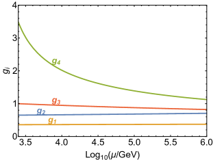
Figure G.1: RGE of the gauge couplings in our benchmark scenario from the TeV scale to the scale of the twin Pati-Salam symmetry $\mu\sim 1\,\mathrm{PeV}$.

References

- (1) LHCb collaboration, R. Aaij et al., Test of lepton universality with decays, JHEP 08 (2017) 055 [1705.05802].
- (2) LHCb collaboration, R. Aaij et al., Test of lepton universality in beauty-quark decays, Nature Phys. 18 (2022) 277 [2103.11769].
- (3) HFLAV collaboration, Y. Amhis et al., Averages of -hadron, -hadron, and -lepton properties as of 2021, 2206.07501.
- (4) A. Crivellin, G. D’Ambrosio and J. Heeck, Explaining , and in a two-Higgs-doublet model with gauged , Phys. Rev. Lett. 114 (2015) 151801 [1501.00993].
- (5) A. Crivellin, G. D’Ambrosio and J. Heeck, Addressing the LHC flavor anomalies with horizontal gauge symmetries, Phys. Rev. D 91 (2015) 075006 [1503.03477].
- (6) C.-W. Chiang, X.-G. He, J. Tandean and X.-B. Yuan, and related anomalies in minimal flavor violation framework with boson, Phys. Rev. D 96 (2017) 115022 [1706.02696].
- (7) S. F. King, Flavourful models for , JHEP 08 (2017) 019 [1706.06100].
- (8) A. Falkowski, S. F. King, E. Perdomo and M. Pierre, Flavourful portal for vector-like neutrino Dark Matter and , JHEP 08 (2018) 061 [1803.04430].
- (9) M. Fernández Navarro and S. F. King, Fermiophobic model for simultaneously explaining the muon anomalies and , Phys. Rev. D 105 (2022) 035015 [2109.08729].
- (10) D. Bečirević and O. Sumensari, A leptoquark model to accommodate and , JHEP 08 (2017) 104 [1704.05835].
- (11) I. de Medeiros Varzielas and S. F. King, with leptoquarks and the origin of Yukawa couplings, JHEP 11 (2018) 100 [1807.06023].
- (12) A. Angelescu, D. Bečirević, D. A. Faroughy, F. Jaffredo and O. Sumensari, Single leptoquark solutions to the B-physics anomalies, Phys. Rev. D 104 (2021) 055017 [2103.12504].
- (13) D. Bečirević, I. Doršner, S. Fajfer, D. A. Faroughy, F. Jaffredo, N. Košnik et al., On a model with two scalar leptoquarks – and , 2206.09717.
- (14) J. C. Pati and A. Salam, Lepton Number as the Fourth Color, Phys. Rev. D 10 (1974) 275.
- (15) B. Diaz, M. Schmaltz and Y.-M. Zhong, The leptoquark Hunter’s guide: Pair production, JHEP 10 (2017) 097 [1706.05033].
- (16) L. Di Luzio, A. Greljo and M. Nardecchia, Gauge leptoquark as the origin of B-physics anomalies, Phys. Rev. D 96 (2017) 115011 [1708.08450].
- (17) H. Georgi and Y. Nakai, Diphoton resonance from a new strong force, Phys. Rev. D 94 (2016) 075005 [1606.05865].
- (18) L. Di Luzio, J. Fuentes-Martin, A. Greljo, M. Nardecchia and S. Renner, Maximal Flavour Violation: a Cabibbo mechanism for leptoquarks, JHEP 11 (2018) 081 [1808.00942].
- (19) C. Cornella, J. Fuentes-Martin and G. Isidori, Revisiting the vector leptoquark explanation of the B-physics anomalies, JHEP 07 (2019) 168 [1903.11517].
- (20) C. Cornella, D. A. Faroughy, J. Fuentes-Martin, G. Isidori and M. Neubert, Reading the footprints of the B-meson flavor anomalies, JHEP 08 (2021) 050 [2103.16558].
- (21) S. F. King, Twin Pati-Salam theory of flavour with a TeV scale vector leptoquark, JHEP 11 (2021) 161 [2106.03876].
- (22) M. Bordone, C. Cornella, J. Fuentes-Martin and G. Isidori, A three-site gauge model for flavor hierarchies and flavor anomalies, Phys. Lett. B 779 (2018) 317 [1712.01368].
- (23) M. Bordone, C. Cornella, J. Fuentes-Martín and G. Isidori, Low-energy signatures of the model: from -physics anomalies to LFV, JHEP 10 (2018) 148 [1805.09328].
- (24) J. Fuentes-Martin, G. Isidori, J. M. Lizana, N. Selimovic and B. A. Stefanek, Flavor hierarchies, flavor anomalies, and Higgs mass from a warped extra dimension, Phys. Lett. B 834 (2022) 137382 [2203.01952].
- (25) L.-S. Geng, B. Grinstein, S. Jäger, S.-Y. Li, J. Martin Camalich and R.-X. Shi, Implications of new evidence for lepton-universality violation in b→s+- decays, Phys. Rev. D 104 (2021) 035029 [2103.12738].
- (26) W. Altmannshofer and P. Stangl, New physics in rare B decays after Moriond 2021, Eur. Phys. J. C 81 (2021) 952 [2103.13370].
- (27) LHCb collaboration, Test of lepton universality in decays, 2212.09152.
- (28) M. Bordone, G. Isidori and A. Pattori, On the Standard Model predictions for and , Eur. Phys. J. C 76 (2016) 440 [1605.07633].
- (29) LHCb collaboration, Measurement of the ratios of branching fractions and , 2302.02886.
- (30) S. F. King, A Simplified Twin Pati-Salam Theory of Flavour with a TeV Scale Vector Leptoquark, in 21st Hellenic School and Workshops on Elementary Particle Physics and Gravity, 3, 2022, 2203.02236.
- (31) G. Valencia and S. Willenbrock, Quark - lepton unification and rare meson decays, Phys. Rev. D 50 (1994) 6843 [hep-ph/9409201].
- (32) Particle Data Group collaboration, R. L. Workman, Review of Particle Physics, PTEP 2022 (2022) 083C01.
- (33) R. A. Porto and A. Zee, The Private Higgs, Phys. Lett. B 666 (2008) 491 [0712.0448].
- (34) R. A. Porto and A. Zee, Neutrino Mixing and the Private Higgs, Phys. Rev. D 79 (2009) 013003 [0807.0612].
- (35) Y. BenTov and A. Zee, Private Higgs at the LHC, Int. J. Mod. Phys. A 28 (2013) 1350149 [1207.0467].
- (36) W. Rodejohann and U. Saldaña Salazar, Multi-Higgs-Doublet Models and Singular Alignment, JHEP 07 (2019) 036 [1903.00983].
- (37) R. Barbieri, C. Cornella and G. Isidori, Simplified models of vector leptoquarks at the TeV, 2207.14248.
- (38) L. Di Luzio, M. Kirk, A. Lenz and T. Rauh, theory precision confronts flavour anomalies, JHEP 12 (2019) 009 [1909.11087].
- (39) K. Hayasaka et al., Search for Lepton Flavor Violating Tau Decays into Three Leptons with 719 Million Produced Tau+Tau- Pairs, Phys. Lett. B 687 (2010) 139 [1001.3221].
- (40) HFLAV collaboration, Y. S. Amhis et al., Averages of b-hadron, c-hadron, and -lepton properties as of 2018, Eur. Phys. J. C 81 (2021) 226 [1909.12524].
- (41) LHCb collaboration, R. Aaij et al., Search for the lepton-flavour-violating decays and , Phys. Rev. Lett. 123 (2019) 211801 [1905.06614].
- (42) BaBar collaboration, J. P. Lees et al., A search for the decay modes , Phys. Rev. D 86 (2012) 012004 [1204.2852].
- (43) Belle collaboration, Y. Miyazaki et al., Search for Lepton-Flavor-Violating tau Decays into a Lepton and a Vector Meson, Phys. Lett. B 699 (2011) 251 [1101.0755].
- (44) LHCb collaboration, R. Aaij et al., Search for the decays and , Phys. Rev. Lett. 118 (2017) 251802 [1703.02508].
- (45) BaBar collaboration, J. P. Lees et al., Search for at the BaBar experiment, Phys. Rev. Lett. 118 (2017) 031802 [1605.09637].
- (46) BaBar collaboration, J. P. Lees et al., Search for and invisible quarkonium decays, Phys. Rev. D 87 (2013) 112005 [1303.7465].
- (47) Belle collaboration, J. Grygier et al., Search for decays with semileptonic tagging at Belle, Phys. Rev. D 96 (2017) 091101 [1702.03224].
- (48) CMS collaboration, C. Kar, Recent Measurement on the Properties with CMS Data, Springer Proc. Phys. 277 (2022) 97.
- (49) LHCb collaboration, R. Aaij et al., Analysis of Neutral B-Meson Decays into Two Muons, Phys. Rev. Lett. 128 (2022) 041801 [2108.09284].
- (50) B. Allanach and J. Davighi, The Rumble in the Meson: a leptoquark versus a to fit anomalies including 2022 LHCb measurements, 2211.11766.
- (51) N. Gubernari, M. Reboud, D. van Dyk and J. Virto, Improved theory predictions and global analysis of exclusive processes, JHEP 09 (2022) 133 [2206.03797].
- (52) LHCb collaboration, R. Aaij et al., Measurement of -Averaged Observables in the Decay, Phys. Rev. Lett. 125 (2020) 011802 [2003.04831].
- (53) LHCb collaboration, R. Aaij et al., Angular Analysis of the Decay, Phys. Rev. Lett. 126 (2021) 161802 [2012.13241].
- (54) A. Greljo, J. Salko, A. Smolkovič and P. Stangl, Rare decays meet high-mass Drell-Yan, 2212.10497.
- (55) M. Ciuchini, M. Fedele, E. Franco, A. Paul, L. Silvestrini and M. Valli, Constraints on Lepton Universality Violation from Rare Decays, 2212.10516.
- (56) M. Algueró, B. Capdevila, S. Descotes-Genon, J. Matias and M. Novoa-Brunet, global fits after and , Eur. Phys. J. C 82 (2022) 326 [2104.08921].
- (57) C. Bobeth, U. Haisch, A. Lenz, B. Pecjak and G. Tetlalmatzi-Xolocotzi, On new physics in , JHEP 06 (2014) 040 [1404.2531].
- (58) B. Capdevila, A. Crivellin, S. Descotes-Genon, L. Hofer and J. Matias, Searching for New Physics with processes, Phys. Rev. Lett. 120 (2018) 181802 [1712.01919].
- (59) A. Crivellin, C. Greub, D. Müller and F. Saturnino, Importance of Loop Effects in Explaining the Accumulated Evidence for New Physics in B Decays with a Vector Leptoquark, Phys. Rev. Lett. 122 (2019) 011805 [1807.02068].
- (60) M. Algueró, J. Matias, B. Capdevila and A. Crivellin, Disentangling lepton flavor universal and lepton flavor universality violating effects in b→s+- transitions, Phys. Rev. D 105 (2022) 113007 [2205.15212].
- (61) J. Fuentes-Martín, G. Isidori, M. König and N. Selimović, Vector Leptoquarks Beyond Tree Level III: Vector-like Fermions and Flavor-Changing Transitions, Phys. Rev. D 102 (2020) 115015 [2009.11296].
- (62) Belle-II collaboration, W. Altmannshofer et al., The Belle II Physics Book, PTEP 2019 (2019) 123C01 [1808.10567].
- (63) J. Fuentes-Martín and P. Stangl, Third-family quark-lepton unification with a fundamental composite Higgs, Phys. Lett. B 811 (2020) 135953 [2004.11376].
- (64) M. J. Dolan, T. P. Dutka and R. R. Volkas, Lowering the scale of Pati-Salam breaking through seesaw mixing, JHEP 05 (2021) 199 [2012.05976].
- (65) LHCb collaboration, R. Aaij et al., Physics case for an LHCb Upgrade II - Opportunities in flavour physics, and beyond, in the HL-LHC era, 1808.08865.
- (66) F. Goertz, J. F. Kamenik, A. Katz and M. Nardecchia, Indirect Constraints on the Scalar Di-Photon Resonance at the LHC, JHEP 05 (2016) 187 [1512.08500].
- (67) M. J. Baker, J. Fuentes-Martín, G. Isidori and M. König, High- signatures in vector–leptoquark models, Eur. Phys. J. C 79 (2019) 334 [1901.10480].
- (68) J. Fuentes-Martín, G. Isidori, M. König and N. Selimović, Vector Leptoquarks Beyond Tree Level, Phys. Rev. D 101 (2020) 035024 [1910.13474].
- (69) J. Fuentes-Martín, G. Isidori, M. König and N. Selimović, Vector leptoquarks beyond tree level. II. corrections and radial modes, Phys. Rev. D 102 (2020) 035021 [2006.16250].
- (70) J. Alwall, R. Frederix, S. Frixione, V. Hirschi, F. Maltoni, O. Mattelaer et al., The automated computation of tree-level and next-to-leading order differential cross sections, and their matching to parton shower simulations, JHEP 07 (2014) 079 [1405.0301].
- (71) A. Alloul, N. D. Christensen, C. Degrande, C. Duhr and B. Fuks, FeynRules 2.0 - A complete toolbox for tree-level phenomenology, Comput. Phys. Commun. 185 (2014) 2250 [1310.1921].
- (72) CMS collaboration, A. M. Sirunyan et al., Search for high mass dijet resonances with a new background prediction method in proton-proton collisions at 13 TeV, JHEP 05 (2020) 033 [1911.03947].
- (73) ATLAS collaboration, M. Aaboud et al., Search for new high-mass phenomena in the dilepton final state using 36 fb-1 of proton-proton collision data at TeV with the ATLAS detector, JHEP 10 (2017) 182 [1707.02424].
- (74) ATLAS collaboration, M. Aaboud et al., Search for additional heavy neutral Higgs and gauge bosons in the ditau final state produced in 36 fb-1 of pp collisions at TeV with the ATLAS detector, JHEP 01 (2018) 055 [1709.07242].
- (75) CMS collaboration, The search for a third-generation leptoquark coupling to a lepton and a b quark through single, pair and nonresonant production at , tech. rep., CERN, Geneva, 2022.
- (76) CMS collaboration, Search for pair-produced vector-like leptons in final states with third-generation leptons and at least three b quark jets in proton-proton collisions at = 13 TeV, 2208.09700.
- (77) A. Greljo and B. A. Stefanek, Third family quark–lepton unification at the TeV scale, Phys. Lett. B 782 (2018) 131 [1802.04274].
- (78) S. Fajfer, A. Greljo, J. F. Kamenik and I. Mustac, Light Higgs and Vector-like Quarks without Prejudice, JHEP 07 (2013) 155 [1304.4219].
- (79) S. J. D. King, S. F. King, S. Moretti and S. J. Rowley, Discovering the origin of Yukawa couplings at the LHC with a singlet Higgs and vector-like quarks, JHEP 21 (2020) 144 [2102.06091].
- (80) B. Grzadkowski, M. Iskrzynski, M. Misiak and J. Rosiek, Dimension-Six Terms in the Standard Model Lagrangian, JHEP 10 (2010) 085 [1008.4884].
- (81) J. Fuentes-Martin, P. Ruiz-Femenia, A. Vicente and J. Virto, DsixTools 2.0: The Effective Field Theory Toolkit, Eur. Phys. J. C 81 (2021) 167 [2010.16341].
- (82) D. Bečirević, O. Sumensari and R. Zukanovich Funchal, Lepton flavor violation in exclusive decays, Eur. Phys. J. C 76 (2016) 134 [1602.00881].
- (83) S. Bruggisser, R. Schäfer, D. van Dyk and S. Westhoff, The Flavor of UV Physics, JHEP 05 (2021) 257 [2101.07273].
- (84) C. Bobeth, M. Gorbahn, T. Hermann, M. Misiak, E. Stamou and M. Steinhauser, in the Standard Model with Reduced Theoretical Uncertainty, Phys. Rev. Lett. 112 (2014) 101801 [1311.0903].
- (85) Flavour Lattice Averaging Group (FLAG) collaboration, Y. Aoki et al., FLAG Review 2021, Eur. Phys. J. C 82 (2022) 869 [2111.09849].
- (86) LHCb collaboration, R. Aaij et al., Precise determination of the – oscillation frequency, Nature Phys. 18 (2022) 1 [2104.04421].
- (87) Flavour Lattice Averaging Group collaboration, S. Aoki et al., FLAG Review 2019: Flavour Lattice Averaging Group (FLAG), Eur. Phys. J. C 80 (2020) 113 [1902.08191].
- (88) Fermilab Lattice, MILC collaboration, A. Bazavov et al., -mixing matrix elements from lattice QCD for the Standard Model and beyond, Phys. Rev. D 93 (2016) 113016 [1602.03560].
- (89) RBC/UKQCD collaboration, P. A. Boyle, L. Del Debbio, N. Garron, A. Juttner, A. Soni, J. T. Tsang et al., SU(3)-breaking ratios for and mesons, 1812.08791.
- (90) R. J. Dowdall, C. T. H. Davies, R. R. Horgan, G. P. Lepage, C. J. Monahan, J. Shigemitsu et al., Neutral B-meson mixing from full lattice QCD at the physical point, Phys. Rev. D 100 (2019) 094508 [1907.01025].
- (91) M. Kirk, A. Lenz and T. Rauh, Dimension-six matrix elements for meson mixing and lifetimes from sum rules, JHEP 12 (2017) 068 [1711.02100].
- (92) A. G. Grozin, R. Klein, T. Mannel and A. A. Pivovarov, mixing at next-to-leading order, Phys. Rev. D 94 (2016) 034024 [1606.06054].
- (93) D. King, A. Lenz and T. Rauh, Bs mixing observables and |Vtd/Vts| from sum rules, JHEP 05 (2019) 034 [1904.00940].
- (94) G. Buchalla, A. J. Buras and M. E. Lautenbacher, Weak decays beyond leading logarithms, Rev. Mod. Phys. 68 (1996) 1125 [hep-ph/9512380].
- (95) A. E. Cárcamo Hernández, S. F. King, H. Lee and S. J. Rowley, Is it possible to explain the muon and electron in a model?, Phys. Rev. D 101 (2020) 115016 [1910.10734].
- (96) G. Buchalla and A. J. Buras, The rare decays , and : An Update, Nucl. Phys. B 548 (1999) 309 [hep-ph/9901288].
- (97) L. Calibbi, A. Crivellin and T. Li, Model of vector leptoquarks in view of the -physics anomalies, Phys. Rev. D 98 (2018) 115002 [1709.00692].
- (98) M. Blanke and A. Crivellin, Meson Anomalies in a Pati-Salam Model within the Randall-Sundrum Background, Phys. Rev. Lett. 121 (2018) 011801 [1801.07256].