ByteStore: Hybrid Layouts for Main-Memory Column Stores

Abstract

The performance of main memory column stores highly depends on the scan and lookup operations on the base column layouts. Existing column-stores adopt a homogeneous column layout, leading to sub-optimal performance on real workloads since different columns possess different data characteristics. In this paper, we propose ByteStore, a column store that uses different storage layouts for different columns. We first present a novel data-conscious column layout, PP-VBS (Prefix-Preserving Variable Byte Slice). PP-VBS exploits data skew to accelerate scans without sacrificing lookup performance. Then, we present an experiment-driven column layout advisor to select individual column layouts for a workload. Extensive experiments on real data show that ByteStore outperforms homogeneous storage engines by up to 5.2$\times$.

1 Introduction

Main-memory column stores are popular for fast analytics of relational data [1, 2, 3]. By holding the data inside the memory of a server, or the aggregated memory of a cluster, these systems eliminate the disk I/O bottleneck and have the potential to unleash the high performance locked in modern CPU-memory stacks, including multiple cores, simultaneous multi-threading (SMT), single-instruction multiple-data (SIMD) instruction sets, hierarchical cache, and large DRAM bandwidth.

OLAP workloads are usually read-only. To fully utilize the power of column-oriented storage, denormalization is often used to transform tables into one or a few outer-joined wide tables such that expensive joins and nested queries can then be flattened as simple scan-based queries on the relevant columns [4, 5, 6]. Under this scan-heavy paradigm, most of the query time is spent on two operations that directly consume the base columns: scan and lookup. The scan operation on a column filters row IDs whose column values satisfy a predicate (e.g., year < 2018). Given these row IDs, the lookup operation extracts column values into their plain form (e.g., int32) to be consumed by upstream operations, such as sorting [7, 8], aggregation [9], and so on. The overall performance of queries thus heavily depends on the scan and lookup performance on the base columns [5, 6].

Recently, there has been a flurry of research for in-memory base column layouts such as Bit-Packed [10, 11], PE-VBP [6, 12] and ByteSlice [5], which enable fast column scans. From the system perspective, however, all of them are column stores with a homogeneous storage layout, i.e., the same storage layout is used across all data columns. Figure 1 hints the drawback of such a homogeneous approach. In the figure, it shows the scan performance on the state-of-the-art main-memory column layouts: ByteSlice [5] and PE-VBP (stands for Padded Encoding Vertical Bit Packing) [12] on a real dataset [13] with 23 columns. We run the experiments using one core and give performance measurements in terms of processor cycles per column code. It is clear that no one size fits all: PE-VBP, which is skew-aware, outperforms ByteSlice, which is skew-agnostic, on 9 out of 23 columns. Meanwhile, ByteSlice outperforms PE-VBP for the rest. The above motivates us to design ByteStore, a new storage engine for column stores. ByteStore adopts different storage layouts for different data columns. ByteStore is different from other hybrid storage engines like HYRISE [14]. HYRISE uses a hybrid of row/column storage for HTAP workloads. By contrast, ByteStore is a pure column store that focuses on OLAP workload but it is hybrid in terms of using different encoding and layouts to store the columns. To our best knowledge, this paper is the first to use different storage layouts for different base columns in main-memory column stores.

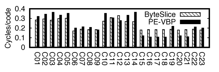
Figure 1: Scan Speed on a Real Dataset: ByteSlice vs PE-VBP

Technically, ByteStore is beyond a simple integration of ByteSlice and PE-VBP — the two most efficient storage layouts to date for non-skewed and skewed data, respectively. First, ByteStore abandons PE-VBP but uses a new storage layout to complement with ByteSlice instead. The problem of PE-VBP is that it actually has poor lookup performance because of its way of storing the bits of a data value in scattered memory locations. Furthermore, PE-VBP indeed has limited performance edge over ByteSlice when scanning skewed data because its way of encoding a column is prefix-free, making almost all values are encoded with a longer code length. Therefore, one contribution of this paper is PP-VBS (stands for Prefix Preserving Variable Byte Slice), a new storage layout that uses byte as the storage unit and a new prefix-preserving method to encode the skewed columns. Unlike ByteSlice, PP-VBS is skew aware. Different from PE-VBP, PP-VBS leverages data skewness to accelerate scans without hurting lookup performance.

With the advent of PP-VBS, we have observed that ByteSlice layout dominates scan and lookup performance on uniform to lightly skewed data columns and PP-VBS dominates the rest. Therefore, ByteStore has to make a binary decision between the two storage layouts for a given data column. Although the decision boundary looks complicated — ByteSlice and PP-VBS outperform each other based on an array of factors such as the workload, value distribution and domain sizes, we observe that there exists a simple yet reliable decision boundary based solely on data skewness. Therefore, another contribution of this paper is an experiment-driven column-layout-advisor based on that observation.

Works on main-memory analytics mostly are evaluated on synthetic data (e.g., TPC-H) [4, 5, 6, 8, 12, 15, 16]. Our last contribution is a comprehensive experimental study based on not only TPC-H but also six open datasets and workloads. Experiments show that ByteStore outperforms any homogeneous storage engines. It therefore validates the effectiveness of having hybrid data layouts at column level. A preliminary version of this paper appears in [5], in which only ByteSlice was discussed and evaluated. In this version, we discusss a full-fledged hybrid storage engine with ByteSlice as one of its components.

The remainder of this paper proceeds as follows: Section 2 contains necessary background information; Section 3 presents the new storage layout PP-VBS; Section 4 presents the column-layout advisor; Section 5 presents the experimental results. Section 6 discusses related works; Section 7 gives the conclusion.

2 Background and Preliminary

2.1 SIMD Instructions

Data-level parallelism is one strong level of parallelism supported by modern processors. Such parallelism is supported by SIMD (single instruction multiple data) instructions, which interact with $S$-bit SIMD registers as a vector of banks. A bank is a continuous section of $b$ bits. In AVX2, $S=256$ and b is $8$, $16$, $32$ and $64$. We adopt these values in this paper since AVX2 is the most widely available in server processors (e.g., from Intel Haswell to TigerLake and AMD), but remark that our techniques can be straightforwardly extended to AVX-512 model. The choice of $b$, the bank width, is on per instruction basis. A SIMD instruction carries out the same operation on the vector of banks simultaneously. For example, the _mm256_add_epi32() instruction performs an 8-way addition between two SIMD registers, which adds eight pairs of 32-bit integers simultaneously. Similarly, the _mm256_add_epi16() instruction performs 16-way addition between two SIMD registers, which adds sixteen pairs of 16-bit short integers simultaneously. The degree of data-level parallelism is $S/b$.

2.2 Scan-based OLAP Framework

Modern analytical column stores transform complex queries into scan-heavy queries on denormalized wide tables [4, 5, 6]. These queries typically have extensive WHERE clauses requiring scan on many columns. A (column-scalar) scan takes as input a dictionary-encoded column, and a predicate of types $=,\neq,>,<,\leq,\geq$, BETWEEN. The scalar literals in the predicates (e.g., 2018 in WHERE year < 2018) are encoded using the same dictionary to encode the column values. By using order-preserving encoding, comparison on codes yields correct result for comparison of the original column values. For predicates involving arithmetic or similarity search (e.g., LIKE predicates on strings), codes have to be decoded before a scan is evaluated in the traditional way.

The scan operation filters all matching column codes, and outputs a result bit vector to indicate the matching row IDs. The bit vector makes it easy to combine scan results in logical expression (conjunction or disjunction), and handle NULL values and three-valued Boolean logic [6]. All prior works on column scan [4, 5, 6, 12, 10, 11] support this bit vector interface, so we follow the same convention in this paper. After scan, column codes involved in projection, aggregation or sorting may need to be retrieved and reconstructed into their canonical forms (e.g., int32). This is called lookup. The lookup operation takes as input an encoded column and a result bit vector from a scan. It then outputs the values as an array (e.g., int32[]).

Under this framework, scan and lookup are the two major operations whose performance directly depend on the base columns’ layouts. Other operations such as sorting and aggregation are independent of the base columns.

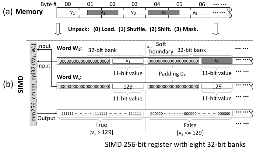
Figure 2: (a) 11-bit column values stored under bit-packed layout (b) Scan on bit-packed data with predicate $v>129$

2.3 Bit-Packed

The Bit-Packed layout [10, 11] aims to minimize the memory bandwidth usage when processing data. Same as ByteSlice, Bit-Packed is skew-agnostic and codes are fixed-length. Figure 2(a) shows an example with 11-bit column codes. Codes are tightly packed together in the memory, ignoring any byte boundaries. To be specific, the first code $v_{1}$ is put in the 1-st to 11-th bits whereas the second code $v_{2}$ is put in the 12-th to 22-nd bits and so on.

To evaluate a scan on a bit-packed column, it is necessary to unpack the tightly packed data into SIMD registers. Since a code may initially span 3 bytes (e.g., $v_{3}$) as shown in Figure 2(a), each code has to be unpacked into a 32-bit bank of the SIMD register. Under AVX2 architecture (i.e., the length of SIMD registers is 256-bit), scan is run in 8-way (256/32) data level parallelism. In other words, eight 11-bit codes (e.g., $v_{1}\sim v_{8}$) are loaded from memory and aligned into eight 32-bit banks of the register. After unpacking, data in the SIMD register (e.g., $W_{1}$ in Figure 2(b)) is ready to be processed by scan operation. Figures 2(b) shows how to evaluate a predicate $v>129$ on the unpacked codes with AVX2’s 8-way greater-than comparison instruction _mm256_cmpgt_epi32(). After that, the scan starts another iteration to unpack and compare the next 8 codes with $W_{c}$. In the example above, although 8-way parallelism is achieved in data processing, many cycles are actually wasted during unpacking. To align the 8 codes into the eight 32-bit banks, three extra SIMD instructions (i.e., Shuffle, Shift and Mask) are carried out. Furthermore, as 0’s are used to pad up with the SIMD soft boundaries, for above example, any data processing operation is wasting $(32-11)\times 8=168$ bits of computation power per cycle.

To retrieve a code $v_{i}$ from bit-packed layout, one has to gather all bytes that it spans. For example, to look up $v_{3}$, Bytes# 02$\sim$04 are fetched from the memory. As a code may span multiple bytes under the bit-packed format, retrieving one code may incur multiple cache misses, particularly when those bytes span across multiple cache lines.

2.4 PE-VBP

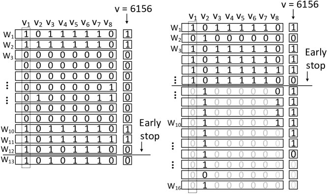
Figure 3: (a) VBP and (b) PE-VBP

Li et al. [12] proposed a variable-length encoding scheme called Padded Encoding (PE) that leverages data skew to accelerate scan. They combine PE with a vertical bit packing (VBP) storage layout [6] to form PE-VBP, a skew-aware column scan technique. Figure 3(a) shows how VBP (without PE) stores a block of eight 13-bit column codes $v_{1}\sim v_{8}$ in memory. Each horizontal box $W_{i}$ is a contiguous memory region. The $j$-th bits of the codes are stored in $W_{j}$. In other words, the bits belonging to $v_{1}=(1100000001111)_{2}$ are vertically distributed across different memory regions (i.e., $W_{1}\sim W_{13}$).

The scan on VBP leverages a key insight that within each processor there is abundant “intra-cycle parallelism” as the processor’s ALU operates on multiple bits in parallel. To illustrate, consider the evaluation of predicate “v = 6156” (see Figure 3(a)). The scan algorithm compares the bits of $v_{i}$ with the bits of 6156 in a bit-by-bit fashion, from the most significant bit to the least significant bit. Since the first bits of $v_{1}\sim v_{8}$ are stored together in $W_{1}$, they can be loaded into the CPU as a single memory word and processed in parallel using bitwise instructions (in real implementation, a memory word is usually a SIMD register, e.g., 256 bits). It compares the first bit of 6156 — $(1)_{2}$ — with all bits in $W_{1}=(10111110)_{2}$. At this point, only the $v_{2}$ and $v_{8}$ are guaranteed to fail the predicate because their first bit is 0. The other six codes are inconclusive. Thus, the scan has to continue to the next (second) bit, and repeats. After scanning the 12-th bits (i.e., $W_{12}$), there are no codes whose first 12 bits match 6156’s first 12 bits, safely declaring all codes in this block (i.e., $v_{1}\sim v_{8}$) fail the predicate. There is no need to load $W_{13}$ into the CPU and process it. In this case, the scan is said to stop early and can proceed to the next block of codes.

PE-VBP builds on VBP by leveraging data skew to increase the chance of early stop during a scan. Similar to Huffman encoding, PE assigns shorter codes for frequent values and longer codes for infrequent values. To store PE-encoded values in VBP, shorter codes are padded with zeros to align with the longest code. Figure 3(b) shows how PE-VBP encodes and stores the same eight column values, where the grey bits are padding zeros. It is worth noting that $v_{1}\sim v_{8}$ are encoded differently from VBP in Figure 3(a). The encoding scheme in PE-VBP is prefix-free, which guarantees that if $a\neq b$, then the encoded value (called code) of $a$ cannot be a prefix of that of $b$, or vice versa. This property increases the maximum length of PE-encoded codes, for example, from 13 to 16 bits in Figure 3.

Despite using more bits, PE-VBP achieves faster scan than VBP when the data is skewed. Figure 3(b) shows the scan can now stop early at the 6-th bits (i.e., $W_{6}$), about $2\times$ faster than VBP, because frequent values $v_{1},v_{3},v_{4},v_{5},v_{6},v_{7}$ are encoded with only 6 bits, as opposed to 13 bits in VBP. In general, PE-VBP increases the likelihood of early stop after scanning each bit. Similar to many existing work [17, 12, 18, 19], PE-VBP uses the Zipf distribution to model skewed data.

Unfortunately, both VBP and PE-VBP suffer from very expensive lookup operation. When reconstructing a column code, both VBP and PE-VBP must retrieve every single bit of a code from a different memory word. Each bit is likely to reside in a different cache line, and incur a cache miss, costing hundreds of CPU cycles. As shown in [5], the expensive lookup often offsets the performance gain of fast scan from the whole query point of view. The problem is exacerbated in PE-VBP since the storage layout of PE-VBP is intrinsically at odds with its variable-length encoding scheme. As shown in Figure 3(b), all short codes have to be padded up with zeros to align with the longest code. It retrieves 16 bits instead of 13 bits in VBP (see Figure 3(a)) to re-build a single code.

2.5 ByteSlice

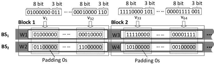
Figure 4: ByteSlice

ByteSlice is a state-of-the-art technique that achieves balanced high performance of scan and lookup. Figure 4 shows how ByteSlice [5] arranges 64 11-bit column codes $v_{1}\sim v_{64}$ in main memory. Each code is chopped into separate bytes. The $j$-th byte of all codes are stored in a continuous memory region. In other words, the bytes of a code $v_{i}$ are vertically distributed in different memory regions. Each of these regions is called a byte slice. At query time, a 256-bit memory word such as $W_{1}$ is loaded into the CPU and processed with byte-level AVX2 SIMD instructions, achieving 32-way parallelism. Similar to VBP, ByteSlice enjoys the benefit of early stop during scan. For example, the scan on Block 1 ($v_{1}\sim v_{32}$) in Figure 4 may stop early after processing $W_{1}$, without needing to load and process $W_{2}$.

ByteSlice is also efficient at lookup. It distributes a $k$-bit code across $\lceil k/8\rceil$ memory words. In Figure 4, a lookup on $v_{i}$ will incur at most 2 memory accesses, as opposed to 11 in VBP. The number $\lceil k/8\rceil$ is typically small (between 1 to 3), so it can be overlapped with other instructions in the CPU’s instruction pipeline [5]. Nonetheless, ByteSlice has not exploited any data skew found in real data. All codes in Figure 4 are encoded into two bytes regardless.

3 PP-VBS

PE-VBP leverages data skew in real data but suffers from poor lookup performance. ByteSlice has excellent balance between scan and lookup but has not leveraged data skew to accelerate its operations. In this section, we present PP-VBS (Prefix Preserving Variable Byte Slice). PP-VBS aims to leverage data skew to accelerate scans without jeopardizing the efficiency of lookups. Similar to ByteSlice and PE-VBP, PP-VBS is a suite of techniques to encode column values into integer codes (Section 3.1), store the codes’ bytes in main memory using a specialized layout (Section 3.2), and perform efficient scan and lookup operations on top (Section 3.3).

3.1 Prefix Preserving Encoding (PPE)

We begin by arguing that the prefix-free property, commonly found in variable-length encoding [20, 21, 22, 23] and used in PE-VBP, is actually unnecessary in the context of main-memory data processing but subverts the performance of both scans and lookups. Traditionally, variable-length encoding schemes were designed for reducing the communication cost when sending a message across the network [21]. In that context, codes are often concatenated as a sequential byte stream, so the prefix-free property is crucial for ensuring the message can be decoded without ambiguity. Concretely, a prefix-free encoding scheme is usually constructed by building a frequency-sorted tree [20]. Figure 5 shows one such example to encode 13 distinct letters of varying frequencies. This tree encodes the values in multiples of two bits, thus having a fan-out of four. The numbers on top of the letters are their frequencies. The bits in the dashed boxes or circles are partial codes. A letter’s code is the concatenation of the bits from the root to its slot. For example, ‘C’ $=(0010)_{2}$, ‘K’ $=(10)_{2}$. When building the tree, values of higher frequencies are assigned to higher slots, thus shorter codes. Scarce values are assigned to lower slots and thus longer codes. The prefix-free property stipulates that a (shorter) code cannot be a prefix of another (longer) code. For example, we cannot use $(\underline{10}01)_{2}$ to encode a letter because $(10)_{2}$ is already assigned to ‘K’. So, in Figure 5, a slot that contains a letter cannot have a pointer to a sub-tree at the same time, nor vice versa.

Code lengths have direct impact on both scan and lookup performance. Firstly, longer codes generally imply more iterations and more instructions during scan. Second, it also implies longer lookup time. By contrast, prefix-preserving encoding (PPE) generally produce shorter codes on average. Figure 6 shows a prefix-preserving example for the same data in Figure 5. These are still variable-length codes, e.g,. ‘A’=$(0001)_{2}$, ‘C’=$(01)_{2}$. A slot can both contain a letter and have a pointer to a sub tree. Note that ‘C’=$(01)_{2}$ does not prevent other codes using it as the prefix, e.g., ‘E’=$(\underline{01}10)_{2}$. In general, PPE achieves smaller frequency-weighted average code length than prefix-free. The average code length in Figure 6 is 2.31 bits as opposed to 3.19 bits in Figure 5. Even though the PPE trees are not always as well balanced as this example, prefix-preserving still allows more values to use short codes and fewer values to use long codes. That in turn allows more values to leverage data skew to accelerate scans and fewer values to suffer from inefficient lookup. The only question is how to deal with ambiguity for codes that share the same prefix. Fortunately, main-memory storage and communication are two very different problems. We can actually store some lightweight disambiguation information elsewhere in the storage level (Section 3.2).

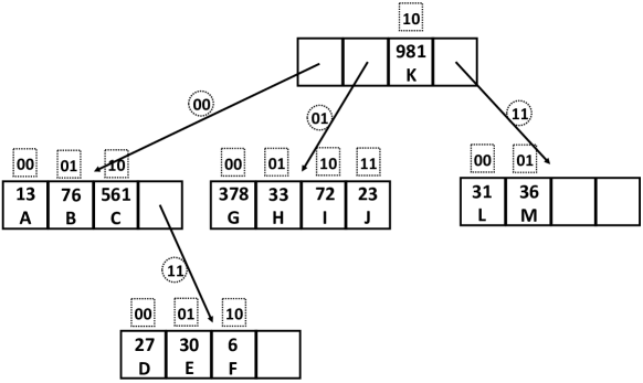
Figure 5: Prefix-free Encoding Tree for Values ‘A’ to ‘M’

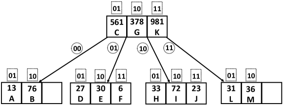
Figure 6: Prefix-preserving Encoding Tree for Value ‘A’ to ‘M’.

PPE is based on building a prefix-preserving $M$-way encoding tree. In Figure 6, $M=4$. Each node in the tree contains $M-1$ slots. Each slot from the left to the right represents a sub-code from $1$ to $M-1$, e.g., from $(01)_{2}$ to $(11)_{2}$ in Figure 6. We call it as slot sub-code, marked in a dashed box. Each non-leaf node has $M$ pointers connecting to $M$ child nodes. Each pointer from the left to the right carries a sub-code from $0$ to $M-1$, e.g., from $(00)_{2}$ to $(11)_{2}$ in Figure 6. We call it pointer sub-code, marked in a dashed circle. Note that slot sub-codes do not start from 0 for the sake of disambiguation, as explained later.

Given an encoding tree, we obtain the encoding of a value $v$ by concatenating all pointer sub-codes on the path from the root to $v$, and $v$’s own slot sub-code. In Figure 6, the code of value ‘C’ is simply its slot sub-code $(01)_{2}$, since it is in the root node; the code of ‘A’ is $(0001)_{2}$, which is formed by concatenation of pointer sub-code $(00)_{2}$ and slot sub-code $(01)_{2}$. Figure 6 also illustrates the intuition of our encoding method: we encode high-frequency values (‘C’, ‘G’, ‘K’) with shorter codes, and low-frequency values with longer codes.

3.1.1 Encoding Numerical Columns (Order-preserving)

In addition to being prefix-preserving, the encoding tree in Figure 6 is also order-preserving. That is, the tree’s in-order traversal gives the ordered sequence of the encoded values. It enables the ordinal comparison of two column values (e.g., ‘A’ vs. ‘C’) by comparing their codes directly (e.g., $(0001)_{2}$ vs. $(01)_{2}$). When comparing two integer codes of different lengths, we treat them as if the shorter code were padded zeros at the end to align with the longer one. Thus, $(0001)_{2}<(01\underline{00})_{2}\Leftrightarrow$ ‘A’ $<$ ‘C’. For this reason, we do not use 0 as slot sub-codes. Otherwise, it cannot differentiate between a short code with padding $(\underset{slot}{\underline{01}}\phantom{0}\underset{pad}{\underline{00}})_{2}$ and a long code $(\underset{pointer}{\underline{01}}\phantom{0}\underset{slot}{\underline{00}})_{2}$. Notice this is different from prefix-free, as there are still prefix-sharing codes (e.g., ‘C’ and ‘E’). Order-preserving is crucial for numerical columns as it enables efficient evaluation of all types of predicates ($=,\neq,<,>,\leq,\geq$) without decoding codes into their represented values.

Input: $n$ distinct values $A$ = $\{A_{0}<A_{1}<...<A_{n-1}\}$, value weights $Q=\{Q_{0},Q_{1},...,Q_{n-1}\}$.

Output: $n$ value codes $C$ = $\{C_{0},C_{1},...,C_{n-1}\}$, code lengths $L$ = $\{L_{0},L_{1},...,L_{n-1}\}$.

1

2

// $b$: the level of the parent node

// $s$: the start index

// $e$: the end index

3 Function PPE_NUMERICAL($C$, $L$, $b$, $s$, $e$):

       // two terminating conditions

4       if $e-s<256$ OR $b\geq 2$ then

5             $\beta=\lceil\log_{256}{(e-s+1)}\rceil$;

6             for $i=s$, …, $e-1$ do

7                   $C_{i}=(C_{i}\ll\beta*8)+1+(i-s)$;
$L_{i}=b+\beta$;

8            

9      else

10             Find the largest 255 frequencies in $Q_{s}\sim Q_{e-1}$, store their indices in an ascending array $I$.

11             for $t=0$, …, $254$ do

12                   $L_{I_{t}}=b+1$;

13                   $C_{I_{t}}=(C_{I_{t}}\ll 8)+t+1$

14                  

15            for $t=0$, …, $253$ do

16                   for $i=I_{t}+1$, …, $I_{t+1}-1$ do

17                         $C_{i}=(C_{i}\ll 8)+t+1$;

18                        

19                  PPE_NUMERICAL($C$, $L$, $b+1$, $I_{t}+1$, $I_{t+1}$);

20                  

            // Deal with the leftmost sub-tree

21             for $i$ = $s$, …, $I_{0}$ - $1$ do

22                   $C_{i}$ = $C_{i}$ $\ll$ $8$;

23            PPE_NUMERICAL($C$, $L$, $b+1$, $s$, $I_{0}$);

             // Deal with the rightmost sub-tree

24             for $i$ = $I_{254}+1$, …, $e-1$ do

25                   $C_{i}$ = ($C_{i}$ $\ll$ 8) + 255;

26                  

27            PPE_NUMERICAL($C$, $L$, $b+1$, $I_{254}+1$, $e$);

28            

29      

30for($i=0$, …, $n-1$): $C_{i}=0$;

31 for($i=0$, …, $n-1$): $L_{i}=0$;

32 PPE_NUMERICAL($C$, $L$, $0$, $0$, $n$);

33

Algorithm 1 PPE for Numerical Columns

To ensure that we do not underutilize the available short codes, all slots of each non-leaf node in a prefix-preserving encoding tree should be filled with higher-frequency values. For example, the root node in Figure 6 is full of values. Therefore, we build the encoding tree in a depth-first search manner and fill all non-leaf nodes in the paths from the root node to leaf nodes.

Without loss of generality, given a sequence of distinct values in ascending order $A_{0}<A_{1}<\cdots<A_{n-1}$, and their corresponding frequencies $Q=\{Q_{0},Q_{1},\cdots,Q_{n-1}\}$, Algorithm 1 shows the pseudocode of constructing a prefix-preserving encoding (PPE) for numerical columns. The outputs of Algorithm 1 are the codes $C$ and the corresponding code lengths $L$. Algorithm 1 builds a 256-way tree, here $M$ equals to 256(=$2^{8}$), since the code lengths are multiple of 1 byte (8 bits) in our setting. At first, we initialize the elements of $C$ and $L$ as $0$’s (Lines 22-23). Then Algorithm 1 invokes a function PPE_NUMERICAL recursively to construct the encoding tree. Among the parameters passed to PPE_NUMERICAL, $s$ and $e$ represent the start and end index, which indicate that values $A_{s}\sim A_{e-1}$ will be encoded in a sub-tree by this call; $b$ indicates the level of its parent node. At the first round, PPE_NUMERICAL selects the 255 largest frequencies from $Q_{0}\sim Q_{n-1}$ and stores their corresponding array indices in an ascending array $I$ (Line 8), i.e., $I_{0}<I_{1}<...<I_{254}$. These most frequent 255 values will reside in the root node and be encoded as 1-byte codes (Lines 9-11), i.e., $(1)_{10}\sim(255)_{10}$. This ensures the most frequent values are encoded with the shortest 1-byte codes. After that, the values between adjacent slots in the root node will be encoded by building a sub-tree, e.g., the values in the positions [$I_{1}+1,I_{2}$) of the sequence $A$, by calling PPE_NUMERICAL recursively (Lines 12-15). Note the extra efforts to deal with the leftmost and rightmost sub-trees (Lines 16-21). Since a non-leaf node must be full before we create any child nodes by recursion, we can see:

Property 1

All (non-leaf) internal nodes in a prefix-preserving encoding tree are full.

The recursion has two terminating conditions (Line 2):

[$e-s<256$]: It means a leaf node has enough slots to hold all the values $A_{s}\sim A_{e-1}$ pending to be encoded. Then their slot sub-code will be assigned $(1)_{10}\sim(e-s)_{10}$ (Line 5), and their code length will be $b+1$ bytes (Line 6), where $b$ is the level of its parent node. There is no need to compare the frequencies of these values.

[$b\geq 2$]: Under some extreme column distributions, the encoding tree will become unbalanced, which has a negative impact on scan and lookup performance. In order to reduce the maximum code length and alleviate the tree unbalance, after 2 levels, the values in the positions [$s,e$) are packed into one leaf node even though the number of values is larger than $255$ (Lines 3-6). Since in real-world datasets, the number of distinct values of columns (aka domain size) is mainly in the range of ($2^{7},2^{16}$) [6, 10], we believe that the value $2$ is a reasonable threshold.

3.1.2 Encoding Categorical Columns (Non Order-preserving)

While all previous works achieve order-preserving for all columns, we observe extra opportunity by forgoing this property for categorical columns. Typically, categorical columns (e.g, city name, brand name, color) are only involved in equality predicates ($=,\neq$), but not range predicates ($<,>,\leq,\geq$). By omitting the need to handle range predicates, we can build an encoding tree that is more balanced and remove exceptionally long codes.

Given a sequence of distinct values $A=\{A_{0},A_{1},...,A_{n-1}\}$ with descending frequencies $Q=\{Q_{0}>Q_{1}>...>Q_{n-1}\}$, Algorithm 2 shows the pseudocode of PPE for categorical columns. Similarly, the outputs of Algorithm 2 are the codes $C$ and corresponding code lengths $L$. The algorithm builds the encoding tree in a breadth-first search manner. Intuitively, it starts by assigning the 255 most frequent values to the top-level slots (i.e., root node). Then, it assigns the next $256\times 255$ (pointers$\times$slots) most frequent values to the second level. If there are still values to encode, it assigns them to the third level, for up to $256^{2}\times 255$ (pointers${}^{2}\times$slots), and so forth. Therefore, Algorithm 2 bounds the height of the tree by a balanced tree that can hold all values (Line 1). It first fills in the non-leaf nodes level-by-level (Lines 3–8). When filling the possibly non-full last level, it evenly distributes the remaining values among the last level nodes to maximize entropy (Lines 9–15). The order does not matter between codes, assuming no range comparison is needed in the workload. Property 1 holds true for categorical columns. In addition:

Property 2

A PPE tree for categorical columns is balanced.

1

Input: $n$ distinct values $A=\{A_{0},A_{1},...,A_{n-1}\}$, value weights $Q=\{Q_{0}>Q_{1}>...>Q_{n-1}\}$.

Output: $n$ value codes $C=\{C_{0},C_{1},...,C_{n-1}\}$, code lengths $L=\{L_{1},L_{2},...,L_{n-1}\}$.

2

// B: the number of the levels of the balanced tree

3 $B=\lceil\log_{256}(n+1)\rceil$;

4 $\alpha=0$;

5 for $b$ = $1,...,B-1$ do

6       for $c=0,...,256^{b-1}-1$ do

7             for $i=1,...,255$ do

8                   $C_{\alpha}$ = $c\ll 8$ + $i$;

9                   $L_{\alpha}$ = $b$;

10                   $\alpha$ += $1$;

11                  

12            

13      

14for $i=1,...,255$ do

15       for $j=0,...,256^{B-1}-1$ do

16             $c_{\alpha}$ = $j\ll 8+i$;

17             $L_{\alpha}$ = $B$;

18             $\alpha$ += $1$;

19             if $\alpha==n$ then

20                   exit(0);

21                  

22            

23      

Algorithm 2 PPE for Categorical Columns

String columns: It is worth noting that certain string columns will encounter range predicates (e.g.,$<$,$>$) in analytical queries. We regard such string columns as semi-categorical and treat them as same as the numerical columns. In other words, we construct an order-preserving PPE for a semi-categorical column using Algorithm 1. In addition, since it is impossible to carry out a similarity search (LIKE predicate) on the codes directly, in our implementation, the codes are decoded to original strings before a similarity search is evaluated in the traditional way.

3.2 Variable Byte Slice (VBS)

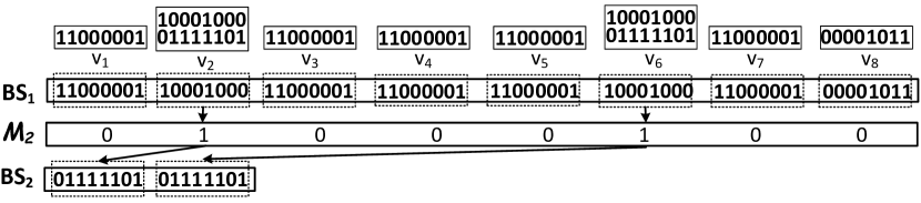
Figure 7: Variable Byte Slice (VBS)

In above, PPE encodes column values into variable-length integer codes logically. Next, Variable Byte Slice (VBS) describes how to store their bits in the main memory physically so that we can perform efficient scan and lookup operations.

Figure 7 gives a quick glimpse of the VBS storage format used in PP-VBS. VBS arranges the $j$-th byte of all codes together in a separate memory region $BS_{j}$. To disambiguate, a bit mask $M_{j}$ indicates whether a code has a materialized $j$-th byte in $BS_{j}$. VBS inherits all good properties of ByteSlice — being amenable to byte-level SIMD instructions and efficient lookup — while bringing in skew-awareness to further improve performance. VBS introduces irregularity that was previously challenging for SIMD processing. We will show how PP-VBS utilizes advanced bit manipulation instructions (e.g., Intel BMI2) in query processing to address those challenges.

Suppose a column of values are encoded with prefix preserving encoding (PPE), VBS vertically distributes the bytes of codes into several contiguous memory regions. Same as [5], we refer to these memory regions as byte slices. If the maximum code length is $K$ bytes, then $K$ byte slices are needed: $BS_{1},BS_{2},$…, $BS_{K}$. Starting from the second byte slice, each byte slice is accompanied with a bitmask indicating whether a code has a (materialized) byte in this slice: $\mathcal{M}_{2},...,\mathcal{M}_{K}$. In other words, VBS packs the $j$-th ($j\geq 2$) bytes of the codes which have the $j$-th byte into $BS_{j}$ tightly. Since all codes have at least one byte, $\mathcal{M}_{1}$ is omitted. Figure 7 illustrates the first $8$ codes of a column under VBS. The maximum code length is two bytes, so there are $2$ byte slices and $1$ bitmask. We use the notation $BS_{j}^{(i)}$ to denote the $i$-th byte in $BS_{j}$. For example, in Figure 7, $BS_{1}^{(2)}=(10001000)_{2}$, $BS_{2}^{(1)}=(01111101)_{2}$. Similarly, we use notation $\mathcal{M}_{j}^{(i)}$ to denote the $i$-th bit in $\mathcal{M}_{j}$: $\mathcal{M}_{2}^{(1)}={(0)}_{2}$, $\mathcal{M}_{2}^{(2)}=(1)_{2}$. In this example, $v_{2}$ and $v_{6}$ have the second byte. Their second bytes are packed together in byte slice $BS_{2}$ with $\mathcal{M}_{2}^{(2)}$ and $\mathcal{M}_{2}^{(6)}$ indicating that information.

Figure 8: A VBS Formatted Column

VBS further divides a column into many blocks. Each block contains data belonging to 32 consecutive codes, under the current implementation using 256-bit AVX2 instructions. Figure 8 illustrates a VBS column having three blocks (96 codes), with maximum code length of 3 bytes. Each horizontal line in the figure represents a contiguous memory region. The dashed line outlines all data belonging to Block 1. Not surprisingly, Block 1 takes up 32 bytes in $BS_{1}$. Among the 32 codes in Block 1, only 10 have the second byte. So Block 1 takes up only 10 bytes in $BS_{2}$. Ditto for $BS_{3}$. In general, $BS_{j}$ always has fewer bytes than $BS_{\{<j\}}$. When data is moderately and highly skewed, a large portion of codes are one byte, and $BS_{\{\geq 2\}}$ have very few bytes. A segment of 32 bits (4 bytes) from the bitmasks $\mathcal{M}_{2}$ and $\mathcal{M}_{3}$ are used to store this sparsity information of Block 1. In summary, Block 1 in VBS uses $4\times 2+32+10+6=56$ bytes, whereas it would have used $32\times 3=96$ bytes in the original ByteSlice.

As discussed in [5, 6, 15, 16], scan is a memory-bound operation. Thus, VBS offers at least two advantages: 1) It reduces memory bandwidth consumption between the memory and the CPU during scan, making it scale on many-core architectures more efficiently. 2) The CPU cache can contain data of more codes, which increases the cache hit rate.

3.3 Scan and Lookup

A PP-VBS scan takes in the VBS column, the predicate operation, and the literal code. It outputs a result bit vector, which indicates the matching rows. Our scan algorithm fully utilizes the data parallelism provided by SIMD instructions. Here, we assume AVX2 architecture is used and the SIMD register is 256-bit. A SIMD instruction carries out the same operation on the vector of banks simultaneously. For example, the _mm256_add_epi8() instruction performs a 32-way addition between two SIMD registers, which adds 32 pairs of 8-bit integers simultaneously. We further exploit advanced bit manipulation instructions such as pdep() and pext() in new generation CPUs to process the bit masks.

3.3.1 Scan

Without loss of generality, we explain with the GREATER-THAN predicate in the form of $v>c$. Other predicate types follow suit. We use the notation $v^{[j]}$ to denote the $j$-th byte of code $v$. For example, in Figure 7, $v_{1}^{[1]}=(11000001)_{2}$, $v_{2}^{[2]}=(01111101)_{2}$. Suppose we have four column codes and a predicate literal $c$ as below:

$\overline{v}_{1}=(10000001~{}\phantom{00000000})_{2}$

$\overline{v}_{2}=(11000000~{}\phantom{00000000})_{2}$

$\overline{v}_{3}=(01110111~{}10101001)_{2}$

$\overline{v}_{4}=(10000001~{}10001001)_{2}$

$c=(10000001~{}\phantom{00000000})_{2}$

The goal of the scan is to determine whether each $\overline{v}$ passes or fails the predicate $\overline{v}>c$. Recall that when comparing two codes of different length, we treat the short code as if it were padded zeros at the end. PP-VBS starts by comparing the first byte of $c$ with the first byte of all $\overline{v}_{i}$:

$\overline{v}_{1}^{[1]}=c^{[1]}$ and $\overline{v}_{2}^{[1]}>c^{[1]}$ and $\overline{v}_{3}^{[1]}<c^{[1]}$ and $\overline{v}_{4}^{[1]}=c^{[1]}$

At this point, we can safely conclude that $\overline{v}_{2}$ passes the predicate, while $\overline{v}_{3}$ fails. There is no need to examine $\overline{v}_{2}$’s and $\overline{v}_{3}$’s second byte. For $\overline{v}_{1}$, we proceed to check its auxiliary bit in $\mathcal{M}_{2}$ (not shown here) to learn that it has no second byte. Hence we know for a fact that $\overline{v}_{1}=c$, meaning $\overline{v}_{1}$ fails the predicate. For $\overline{v}_{4}$, we check its auxiliary bit in $\mathcal{M}_{2}$, and learn that it has a second byte. Without fetching and examining that second byte $\overline{v}_{4}^{[2]}$, we immediately know for a fact that $\overline{v}_{4}>c$, meaning it passes the predicate. That is because, as described in Section 3.1, the last byte (slot sub-code) of a code cannot be zero. Therefore,

$$\overline{v}_{4}=10000001~{}\underset{>0}{\underline{********}}>c=10000001~{}\underset{pad}{\underline{00000000}}$$

In summary, scans on all above codes stop early after the first byte, even though the maximum code length is two. More formally, scan cost on PP-VBS can be bounded by the following lemma:

Lemma 1

Let $l(v)$ be the byte-length of code $v$. For all predicate types $\texttt{op}\in\{<,>,\leq,\geq,=,\neq\}$, the evaluation of predicate $v_{1}~{}\texttt{op}~{}v_{2}$ conclusively stops after examining the $m$-th byte, where $m\leq\min\big{(}l(v_{1}),l(v_{2})\big{)}$.

Proof 1

Let $P_{l}(v)$ denote the $l$-byte prefix of a code $v$. By definition, $v=P_{l(v)}(v)$ for all $v$. Without loss of generality, we assume $l(v_{1})<l(v_{2})$. If we have $P_{l(v_{1})}(v_{1})\leq P_{l(v_{1})}(v_{2})$, then $v_{1}$ must be less than $v_{2}$, because $v_{2}$ must have at least one trailing byte that is larger than 0. If $P_{l(v_{1})}(v_{1})>P_{l(v_{1})}(v_{2})$, we have $v_{2}<P_{l(v_{1})}(v_{2})+1\leq P_{l(v_{1})}(v_{1})\leq v_{1}$. Another special situation is when $l(v_{1})=l(v_{2})$. Under such case, when we have $P_{l(v_{1})}(v_{1})<P_{l(v_{1})}(v_{2})$, then $v_{1}<v_{2}$; when $P_{l(v_{1})}(v_{1})=P_{l(v_{1})}(v_{2})$, then $v_{1}=v_{2}$; when $P_{l(v_{1})}(v_{1})>P_{l(v_{1})}(v_{2})$, then $v_{1}>v_{2}$. Thus, we can compare the prefixes of length $\min(l(v_{1}),l(v_{2}))$ leading bytes to obtain the comparison result between $v_{1}$ and $v_{2}$. This completes the proof.

In addition, PP-VBS inherits the early stop capability of ByteSlice, even when both $v$ and $c$ are long. To illustrate, consider a different predicate literal $c^{\prime}$ for the above example:

$c^{\prime}=(10000000$ $01010000)_{2}$

In this case, after comparing the first byte, we obtain:

$\overline{v}_{1}^{[1]}>c^{\prime[1]}$ and $\overline{v}_{2}^{[1]}>c^{\prime[1]}$ and $\overline{v}_{3}^{[1]}<c^{\prime[1]}$ and $\overline{v}_{4}^{[1]}>c^{\prime[1]}$

which suffices to conclude that $\overline{v}_{1}$, $\overline{v}_{2}$ and $\overline{v}_{4}$ pass the predicate, whereas $\overline{v_{3}}$ fails. There is no need to compare $c^{\prime[2]}$ with any code.

Input: predicate $v>c$; $c$ is $l$-byte;

Output: result bit vector $R$

1 for j = 1,…,l do

2       $W_{cj}=\texttt{simd\_broadcast}(c^{[j]})$

3      

4$I_{j}=0$, for $1\leq j\leq l$

5 for every $S/8$ codes $v_{(I_{1}+1)}...v_{(I_{1}+S/8)}$ do

6       $\mathcal{Z}_{ep}=1^{S/8}$

7       $\mathcal{Z}_{gt}=0^{S/8}$

8       for $j=2,...,\min(l+1,K)$ do

9             $B_{j}=\texttt{load}(\mathcal{M}_{j}^{(I_{1}+1)},...,\mathcal{M}_{j}^{(I_{1}+S/8)})$

10      

11      for $j=1,...,l$ do

12             if $\texttt{test\_zero}(\mathcal{Z}_{eq})$ then

13                   break

14            

15            $W_{j}$ = $\texttt{simd\_load}(BS_{j}^{(I_{j}+1)},...,BS_{j}^{(I_{j}+S/8)})$

16             $M_{gt}$ = $\texttt{simd\_movemask\_epi8}(\texttt{simd\_cmpgt\_epi8}(W_{j},W_{cj}))$

17             $M_{eq}$ = $\texttt{simd\_movemask\_epi8}(\texttt{simd\_cmpeq\_epi8}(W_{j},W_{cj}))$

18             if $j>1$ then

19                   $M_{gt}=\texttt{pdep}(M_{gt},B_{j})$

20                   $M_{eq}=\texttt{pdep}(M_{eq},B_{j})$

21                  

22            if $j<l$ then

23                   $\mathcal{Z}_{gt}=\mathcal{Z}_{gt}|(\mathcal{Z}_{eq}\&M_{gt})$

24                   $\mathcal{Z}_{eq}=\mathcal{Z}_{eq}\&M_{eq}\&B_{j+1}$

25            else if $l<K$ then

26                   $\mathcal{Z}_{gt}=\mathcal{Z}_{gt}|(\mathcal{Z}_{eq}\&M_{gt})|(\mathcal{Z}_{eq}\&M_{eq}\&B_{j+1})$

27            else

28                   $\mathcal{Z}_{gt}=\mathcal{Z}_{gt}|(\mathcal{Z}_{eq}\&M_{gt})$

29            

30      $I_{1}=I_{1}+S/8$

31       for $j=2,...,l$ do

32             $I_{j}=I_{j}+\texttt{POPCNT}(B_{j})$

33      Append $\mathcal{Z}_{gt}$ to $R$

34      

35

Algorithm 3 Vectorized Scan on PP-VBS

Algorithm 3 delineates the VBS’s implementation that “vectorizes” the above scan algorithm to evaluate $S/8=32$ codes in parallel in each iteration using SIMD AVX2 instructions, where the register length $S=256$ bits. The algorithm takes predicate $v>c$ as input and outputs a result bit vector $R$ whose $i$-th bit is $1$ if $v_{i}$ satisfies the predicate or $0$ otherwise. Suppose the constant code $c$ is $l$-byte ($1\leq l\leq K$), $K$ is the maximum code length and the column is numerical. Initially, the bytes of the constant code $c$ are broadcast to $l$ SIMD words (Lines 1-2). Then, the algorithm scans the column codes in a for loop, with one block (32 codes) each time (Lines 4-24). The $i$-th bit of the 32-bit mask $\mathcal{Z}_{gt}$ holds the temporary Boolean value of $v_{i}>c$. Ditto for $\mathcal{Z}_{eq}.$ These two masks are iteratively updated as we examine more bytes of the codes. In order to know which codes in the current block have the $j$-th byte, it loads corresponding auxiliary word $B_{j}$ from $\mathcal{M}_{j}$ (Lines 7-8). The algorithm then examines the codes byte-by-byte through $l$ iterations (Lines 9-24). In the $j$-th iteration, it first tests whether $\mathcal{Z}_{eq}=0$. If yes, the predicate is conclusive for all codes in the block, and thus we can stop early (Lines 10-11). Otherwise, it loads the next $S/8$ bytes from $BS_{j}$ into $W_{j}$, and executes two $S/8$-way SIMD instructions to determine the codes whose $j$-th bytes are either (1)$>$$c^{[j]}$ or (2)$=$$c^{[j]}$. The 256-bit results are condensed into 32-bit bit maps using the movemask instruction (Lines 13–14).

Note that $W_{j}$ may contain bytes belonging to the next block due to sparsity. Concretely, only $T_{j}$ = POPCNT($B_{j}$) $\leq 32$ codes have $j$-th ($j>1$) byte in current block. Thus, only the $T_{j}$ lower bits of $M_{eq},M_{gt}$ in Lines 13–14 are of interest. To put these bits in the right place, we utilize the instruction pdep to scatter the $T_{j}$ consecutive low order bits of $M_{gt}$ and $M_{eq}$ according to $B_{j}$ (Lines 15-17). Figure 9(a) shows an example of pdep instruction. After that, if the $i$-th bit of $B_{j}$ is zero, then the $i$-th bit of $M_{gt}$ and $M_{eq}$ will be $0$. Otherwise, the $i$-th bit in $M_{gt}$ or $M_{eq}$ will indicate whether $j$-th byte of $i$-th code in a block is (1)$>$$c^{[j]}$ or (2)$=$$c^{[j]}$. After processing the current $S/8$ codes, the algorithm must update the indices $I_{j}$ ($1<j\leq l$) to indicate where to load the $j$-th bytes of next block from $BS_{j}$ (Lines 25-27). Finally, the result of current block $\mathcal{Z}_{gt}$ is appended to $R$ (Line 28) before the processing of the next block begins. Algorithm 3 can be easily modified to handle other comparison operators (e.g., $\geq$, $=$), which are omitted in interest of space.

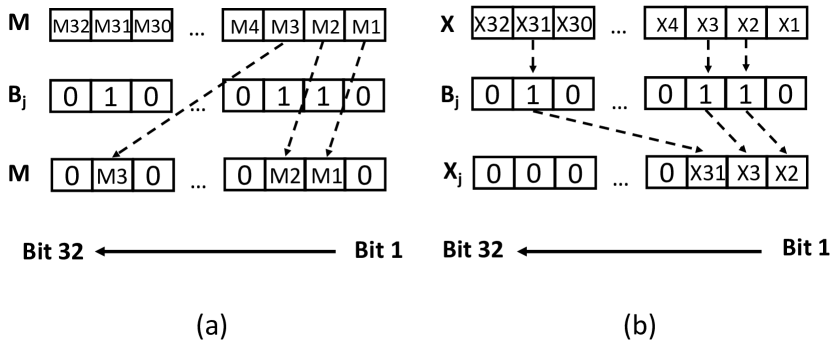
Figure 9: (a) pdep instruction (b) pext instruction

Lemma 1 offers insight why PP-VBS is efficient for skewed columns. Early stop in Algorithm 3 happens per block. Scan on a block can stop early when all $S/8$ codes in it stop early. When the column is more skewed, the probability is higher that all codes in one block are high-frequency values, which are in turn encoded with few bytes under PPE. That bounds the scan cost on every block at a small $m$, even if the literal code $c$ is long.

To handle complex predicates that involve multiple columns, we follow ByteSlice [5] to pipeline the result bit vector of one predicate evaluation to another so as to increase the early stop probability of the subsequent evaluation.

3.3.2 Lookup

Lookup refers to the operation of retrieving the codes from a column of interest given a result bit vector $R$, which is produced by the scan. In the scan-based OLAP framework mentioned in Section 2, the retrieved codes are inserted into an array of a fixed-length data type (e.g., int32[]). Subsequent operations like aggregations and sorts will consume this array. In order to easily embed PP-VBS into this framework, we pad zeros at the end of short codes in the lookup operation to generate fixed-length codes.

Input: $R$: result bit vector; $\mathbb{C}$: a VBS formatted column; $K$: the maximum code length in $\mathbb{C}$

Output: $L$: a list of $K$-byte codes

1 for $1\leq j\leq K$ do

2       $I_{j}=0$;

3for every $\frac{S}{8}$-bit word $x$ in $R$ do

4       for $j=2,...,K$ do

5             $B_{j}=\texttt{load}(\mathcal{M}_{j}^{I_{1}+1},...,\mathcal{M}_{j}^{I_{1}+S/8})$;

6      $\beta=1$;

7       for $j=2,...,K$ do

8             if $\texttt{test\_zero}(x\&B_{j})$ then

9                   break;

10            $\beta=\beta+1$;

11            

12      for $j=2,...,\beta$ do

13             $x_{j}=\texttt{pext}(x,B_{j})$;

14      while $!test\_zero(x)$ do

15            

16            $i=\texttt{POPCNT}(\textbf{P}(x))+1$;

17             $r_{1}=I_{1}+i$;

18             $C=BS_{1}^{(r_{1})}$;

19             $x=\textbf{E}(x)$;

20             for $j=2,...,\beta$ do

21                   if $\texttt{test\_zero}(B_{j}$ $\&$ $(1\ll S/8-i))$ then

22                         $C=C\ll(\beta-j+1)*8$;

23                         break;

24                  $r_{j}=I_{j}+\texttt{POPCNT}(\textbf{P}(x_{j}))+1$;

25                   $C=(C\ll 8)+BS_{j}^{(r_{j})}$;

26                   $x_{j}=\textbf{E}(x_{j});$

27            $C=C\ll(K-\beta)*8$;

28             Append $C$ to $L$;

29            

30      $I_{1}=I_{1}+S/8$;

31       for $j=2,...,K$ do

32             $I_{j}=I_{j}+\texttt{POPCNT}(B_{j})$;

33      

34

Algorithm 4 Lookup Under PP-VBS

Algorithm 4 delineates the pseudo-code of the lookup operation under PP-VBS. It can be seen as the “inverse operation” of VBS. Before formally describing Algorithm 4, we first introduce two bitwise manipulations that provide a fast way to find and manipulate the rightmost 1 bit in a word: (1) $\textbf{E}(x)=x\&(x-1)$, which erases the rightmost $1$ in a word $x$; (2) $\textbf{P}(x)=x\oplus-x$, $\oplus$ is XOR, which propagates the rightmost 1 to the left in the word $x$, making them all 1’s, and erases the rightmost $1$. Here are examples on an 8-bit word $x$.

$x=(010100\underline{1}0)_{2}$

$\textbf{E}(x)=x\&(x-1)=(010100\underline{0}0)_{2}$

$\textbf{P}(x)=x\oplus-x=(111111\underline{0}0)_{2}$

The basic idea behind Algorithm 4 is to extract each $1$ from the result bit vector $R$ and reconstruct the corresponding code from the VBS-formatted column $\mathbb{C}$. To construct a code, we retrieve the bytes from corresponding byte slices and then concatenate them in order. For example, in Figure 7, to obtain 2-byte $v_{2}$, bytes $BS_{1}^{(2)}$ and $BS_{2}^{(1)}$ will be retrieved. When the column is more skewed, the probability is higher that the length of a code retrieved is short so that fewer bytes will be retrieved from the memory.

The algorithm executes in a for loop (Lines 3–26) that handles the result bit vector $R$ in blocks of 32 bits. Let $K$ be the maximum code length in $\mathbb{C}$. $I_{j}$ ($1\leq j\leq K$) tracks the start position of the current block in $BS_{j}$. In each iteration, it loads a $\frac{S}{8}=32$-bit word $x$ from $R$ into CPU. In order to know which codes in the current block have the $j$-th ($j>1$) byte, the algorithm loads the associated auxiliary word $B_{j}$ from $\mathcal{M}_{j}$ (Lines 4–5) . It then determines the (local) maximum length of codes which are extracted in the current block (Lines 7–10) as $\beta$. So it knows which byte slices will be touched and skips processing the rest. Next, the algorithm uses pext instruction to pack bits from the word $x$ according to $B_{j}$ ($2\leq j\leq\beta$) into contiguous low bits of a destination word $x_{j}$ (Lines 11–12). Figure 9(b) shows an example of the pext instruction. A bit set in $x_{j}$ indicates one byte will be retrieved from $BS_{j}$ for constructing a code that is selected in $R$.

Then we iteratively find the rightmost ‘1’ in $x$, calculate its position using POPCNT$(\textbf{P}(\cdot))$, and erase it from $x$ (Lines 14–17). Each popped ‘1’ indicates a code to be reconstructed. The offset is added to tracking index $I_{1}$ to obtain $r_{1}$, which is the position of that code’s first byte in $BS_{1}$ (Line 15). For the $j_{\{>1\}}$-th byte, it first inspects whether the code has the $j$-th byte. If so, it retrieves the $j$-th byte from $BS_{j}$ (Lines 22–24) and concatenates it to $C$. After constructing $C$, we pad zeros at its end and append $C$ to the list $L$ (Lines 25–26). The above procedure repeats until $x=0$, meaning all wanted codes are reconstructed. After one $\frac{S}{8}$-bit word $x$ has been consumed, we update every tracking indices $I_{j}$ ($1\leq j\leq K$).

4 Column-Layout Advisor

(a) Column “Seconds” (Numeric)

(b) Column “Total” (Numeric)

(c) Column “Pickup Census Tract” (Categorical)

Figure 10: Scan Profiles for 3 Real Data Columns from the TAXI_TRIP [13]

As our experiments show in Section 5.1, Bit-Packed and PE-VBP storage layouts are dominated by ByteSlice or PP-VBS in terms of scan and lookup performance. Therefore, given a data column, ByteStore only has to make a decision to store it in ByteSlice or PP-VBS format. Since both ByteSlice and PP-VBS leverage byte as the storage unit, their lookup performances are equally good. Therefore, the decision mainly lies on which one yields better performance on scan.

There are a variety of factors that influence the scan performances of ByteSlice and PP-VBS. Data-related factors include the data distribution type (e.g., Zipf, Gaussian), the parameters (e.g., the Zipf factor), the domain size, and the value type (e.g., numeric or categorical). Query-related factors include the predicate type (e.g., $>$, $=$) and its selectivity (percentage of codes that satisfy the predicate).

Although modeling the relationship between the scan performance and the factors above is challenging, ByteStore does not need to do so because the data columns are actually given. Therefore, the column-layout advisor of ByteStore goes for an experiment-driven approach [24] that chooses the best storage layout for each column based on running (scan) experiments on them. Specifically, given a data column, we first encode it twice: one using ByteSlice and one using PP-VBS; and then we generate and execute scan queries with different selectivities on top to get a profile. Finally, we choose the storage layout of a column based on its profile.

Figure 10 depicts the profiles of three real columns from the TAXI_TRIP [13] real dataset obtained from Google BigQuery. For numeric columns, we use $<$ c as the profiling predicate because from Section 3.3 we know that the scan implementations of other operators (e.g,. $=$) are largely similar and thus their scan performance is also similar (our experiments also confirm this). For categorical columns, we use $=$ c as the profiling predicate. Each profile is obtained by generating and executing queries with 100 predicate literals from the column that span across the entire feasible selectivity spectrum. For example, Figure 10c shows that the most unselective value in the categorical column “Pickup Census Tract” would retrieve 9.9% of the column. All other values have lower selectivity than that.

After profiling, our column-layout advisor computes and picks the one with a smaller area under curve (AUC). For example, it is obvious that for the column “Seconds” in the TAXI_TRIP dataset (Figure 10(a)), the AUC of PP-VBS is smaller than ByteSlice (because that column is skewed). Therefore, the column layout advisor would retain that column encoded using PP-VBS and discard the one encoded using ByteSlice. For the column “Total” in the TAXI_TRIP dataset (Figure 10(b)), our column-layout advisor would also retain the one encoded using PP-VBS because it outperforms ByteSlice for a wide range of selectivities. Of course, if the (range of the) selectivity of a predicate is known, it is straightforward for our advisor to include that factor into account. Algorithm 5 summarizes our discussion above in the form of pseudo-code.

Input: $\mathcal{C}$: a $d$-column dataset, $\mathcal{C}=\{\mathcal{C}_{1},\mathcal{C}_{2},...,\mathcal{C}_{d}\}$.

Output: $\mathcal{L}$: layouts for each column, $\mathcal{L}=\{\mathcal{L}_{1},\mathcal{L}_{2},...,\mathcal{L}_{d}\}$.

1 for j = 1, …, d do

2       Encode $\mathcal{C}_{j}$ with dictionary encoding and inject the column codes into ByteSlice, get $\mathfrak{C}_{j}$.
Encode $\mathcal{C}_{j}$ with prefix preserving encoding and inject the column codes into VBS, get $\mathbb{C}_{j}$.

3      if $\mathcal{C}_{j}$ is numerical then

4             Set predicate $\mathcal{P}$ as $<$.

5      else

6             Set predicate $\mathcal{P}$ as $=$.

7      Select 100 values $\{v_{i}\}_{i=1}^{100}$ from the column $\mathcal{C}_{j}$ that span across the entire feasible selectivity spectrum and the corresponding selectivities are $\{s_{i}\}_{i=1}^{100}$.
Evaluate predicate $\mathcal{P}$ on $\mathfrak{C}_{j}$ with literals $\{v_{i}\}_{i=1}^{100}$ and get 100 (selectivity, time) points, $\{(s_{i},y_{i})\}_{i=1}^{100}$.
Evaluate predicate $\mathcal{P}$ on $\mathbb{C}_{j}$ with literals $\{v_{i}\}_{i=1}^{100}$ and get 100 (selectivity, time) points, $\{(s_{i},z_{i})\}_{i=1}^{100}$.
Fit the performance curve with $\{(s_{i},y_{i})\}_{i=1}^{100}$ and obtain the AUC (area under the curve) $\mathcal{Y}$.
Fit the performance curve with $\{s_{i},z_{i})\}_{i=1}^{100}$ and obtain the AUC (area under the curve) $\mathcal{Z}$. if $\mathcal{Y}$ $\leq$ $\mathcal{Z}$ then

8             $\mathcal{L}_{j}$ = ByteSlice.

9      else

10             $\mathcal{L}_{j}$ = PP - VBS.

11      

Algorithm 5 Column Layout Advisor

5 Experimental Evaluation

We run our experiments on a rack server with a 2.1GHz 8-core Intel Xeon CPU E5-2620 v4, and 64GB DDR4 memory. Each core has 32KB L1i cache, 32KB L1d cache and 256KB L2 unified cache. All cores share a 20MB L3 cache. The CPU is based on Broadwell microarchitecture and supports AVX2 instruction set. In the micro-benchmark evaluation, we compare PP-VBS with Bit-Packed, PE-VBP and ByteSlice to show that PP-VBS is dominating on skewed columns. In the real data evaluation, we show that queries on ByteStore outperform any homogeneous storage engines. Unless stated otherwise, all experiments are run using one core.

5.1 Micro-Benchmark Evaluation

For the first experiment, we create a column with one billion numeric values. The column values are integer numbers in the range of [$0,2^{d}$). Following PE-VBP [12], we generate the column values from the Zipf distribution.

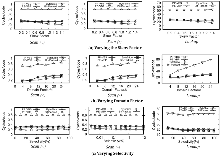
Figure 11: Sensitivity Analysis

Dataset	# of Rows	# of Columns (ByteSlice:PP-VBS)	Encoding Time	Profiling & Layout Selection Time	# of Public Queries
TAXI_TRIP [13]	185,666k	23 (6:17)	180.21 min	12.25 min	3
HEALTH [25]	002,784k	6 (4:2)	001.12 min	00.15 min	1
NYC [26]	146,113k	19 (13:6)	117.16 min	08.03 min	3
EDUCATION [27]	005,082k	6 (3:3)	001.98 min	00.21 min	1
FEC [28]	020,557k	35 (20:15)	030.59 min	02.58 min	2
NPPES [29]	005,943k	480 (353:127)	123.88 min	15.92 min	2

TABLE I: Real Datasets: Characteristics and Ingestion Time/Result

Figure 11(a) reports the scan and lookup performance of different layouts when varying skew factor. The results are averages from queries with 100 different selectivities. In this experiment, following [12], we set the domain size as $2^{12}$ (i.e., $d=12$). It is reasonable since in real-world datasets, the number of distinct values of columns (aka domain size) is mainly in the range of ($2^{7}$,$2^{16}$) [6, 10]. As shown in Figure 11(a), ByteSlice is dominant on scan operation when the skew factor is less than 0.5; PP-VBS starts to dominate when the skew factor increases. PP-VBS, ByteSlice and PE-VBP achieve way better scan performance than Bit-Packed layout because of early stop. In terms of lookup, PP-VBS and ByteSlice perform as well as Bit-Packed and outperform PE-VBP in all cases because they do not scatter the bits into so many different words as PE-VBP does. Lookup performance on PP-VBS improves mildly when the data is getting more skewed because averagely each block of a column contains more short-length codes under higher skew. It decreases the number of bytes read from the memory, which benefits the memory-bound lookup operation.

Figure 11(b) reports the scan and lookup performance of different layouts when varying the domain size (i.e., $2^{4}\sim 2^{24}$). We fix the skew factor as 1.0 in this experiment. On skewed data, PP-VBS outperforms Bit-Packed, PE-VBP and ByteSlice under a wide range of domain size in terms of scan operation. The cost of scan increases with the domain size because generally more bits of a code are retrieved from the memory for a predicate. Lookup time also increases with the domain size because the average code length increases with domain size.

Figure 11(c) reports the scan and lookup performance of different layouts when varying selectivities. We fix skew factor as 1.0 and domain size as $2^{12}$ (i.e., $d=12$) in this experiment. PP-VBS dominates all the other storage layouts on scan for all selectivities. Both PP-VBS and ByteSlice also have as excellent performance as Bit-Packed and outperform PE-VBP on lookup operation under all selectivites.

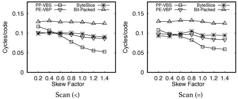
Figure 12: Multi-threaded Scan (#threads = 8)

In addition, we evaluated our experiments of multiple threads. Figure  12 reports the scan performance of different layouts when varying skew factor. In this experiment, we fixed the domain size as $2^{12}$ (i.e., $d$ = 12) and the number of threads as $8$, which means all CPU cores are used. It is clear to see that we can draw similar conclusion from the multi-threaded experiments to that from the single-threaded counterpart.

we also have carried out experiments of (i) varying the cardinalities of the columns, (ii) using data generated by Gaussian distribution of different variances instead of using Zipf distribution, (iii) using other operators (e.g., $\geq$). Since those experiments draw similar conclusions as the above, we do not present them here for space interest.

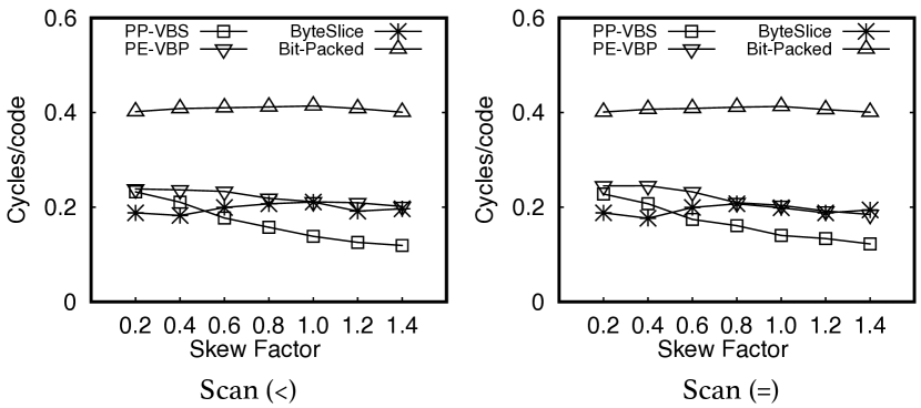
Figure 13: Scan Performance with AVX-512

AVX-512: Our techniques are not specific to AVX2, they can be straightforwardly extended to AVX-512 model. We re-implemented PP-VBS, Bit-Packed, PE-VBP and ByteSlice with AVX-512 instructions (e.g., _mm512_cmpgt_epu8_mask() ) and ran the experiments on a 2.2GHz 10-core Intel Xeon Silver 4114 processor. Figure 13 reports the scan performance of different layouts when varying skew factor using single core. Domain size is fixed as $2^{12}$ in this experiment. We can obtain the similar conclusion that ByteSlice is dominant on scan operation when the skew factor is less than 0.5; PP-VBS starts to dominate when the skew factor increases.

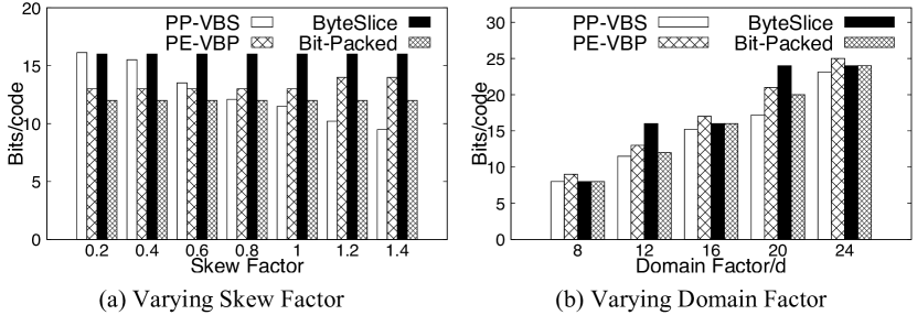
Figure 14: Memory Usage of Different Layouts

Memory Usage: Figure 14 reports the average number of bits used per code under different storage layouts. In Figure 14(a), we fixed the domain size as $2^{12}$ and varied the skew factor. Not surprisingly, the average number of bits per code under PP-VBS reduces as the skew factor increases and PP-VBS starts to dominate other storage layouts when the skew factor is larger than 0.8. Notably, we also counted the memory usage of the bitmasks $\mathcal{M}$. The memory usage of PE-VBP increases along with the skew factor since the maximum code length increases with the skew factor. For ByteSlice, even though the code length is 12-bit, one code must take up 16 bits under ByteSlice because of padding zeros, which will waste memory. However, we focus on scan and lookup performance in this paper and select ByteSlice as a candidate since it dominates scan and lookup performance on uniform to lightly skewed data columns. As opposite to Figure 14(a), we fixed the skew factor as $1$ and varied the domain factor in Figure 14(b). PP-VBS uses the least memory when columns are skewed under varying domain factor.

5.2 Real Data Evaluation

This set of experiments aims to evaluate ByteStore as a whole and compare it with homogenous storage engines that use only Bit-Packed, use only ByteSlice or only PE-VBP.

The experiments are done using 6 real datasets downloaded from Google BigQuery in 2019 May [30]. Table I shows their details as well as the results of dataset ingestion by ByteStore’s column layout advisor. It clearly shows that different columns in a dataset require different storage layouts. The column layout advisor does not use much time to do the profiling and layout selection. The offline data ingestion time is mainly spent on encoding the columns, but half of that time is indispensable as the column has to be encoded in one of the two storage layouts anyway. To focus only on scans and lookups, we follow [4] to materialize the joins and execute the selection-projection components of the queries. Same as [5], we discard the queries that have no selection clause and queries that involve string similarity comparison LIKE. In interest of space, the details of these queries are not presented, please refer to the main page of each dataset for more information.

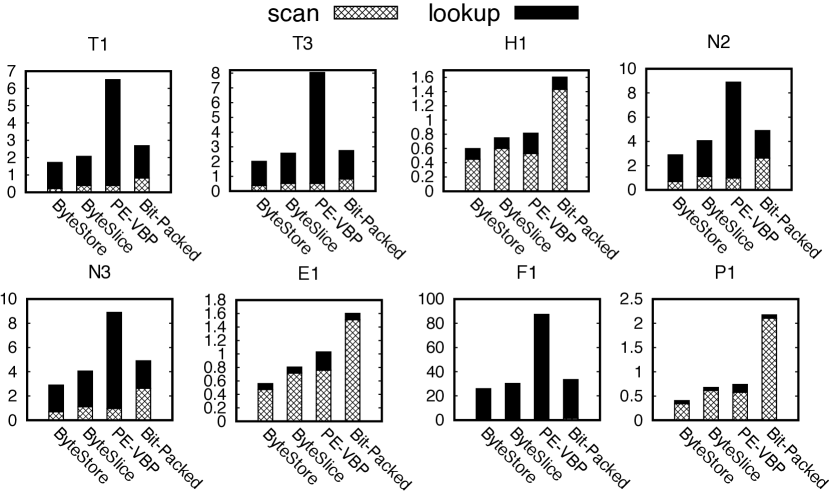
(a) Execution Time Breakdown for Queries. Y-axis reports cycles per tuple

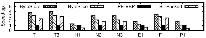
(b) Query Speed-up Over PE-VBP

Figure 15: Performance Comparison of Different Layouts on Six Real Datasets: TAXITRIP(Queries T*), HEALTH (Queries H*), NYC(Queries N*), EDUCATION (Queries E*), FEC (Queries F*), NPPES (Queries P*)

Figure 15 compares ByteStore with using ByteSlice only, using PE-VBP only, and using Bit-Packed only across different queries and different datasets. In Figure 15(a), we report the execution time breakdown of all queries. The run time of each query is dissected into scan cost and lookup cost. The reported numbers have been normalized on a per tuple basis. We could see there are both scan-dominant (e.g., E1 and P1) and lookup-dominant (e.g., F1) queries. We can see that ByteStore outperforms all homogeneous storage schemes. Figure 15(b) reports the query speed-up over PE-VBP only. Overall, ByteStore brings up to 4.0$\times$, 1.7$\times$ and 5.2$\times$ speedup to query performance when comparing with using PE-VBP only, ByteSlice only and Bit-Packed only respectively.

6 Related Work

Since the beginning of 21st century, there have been several hybrid data engines developed for HTAP workloads. Hybrid storage engines mainly focus on mixing the row and column representations [31, 32, 33, 34, 35, 36, 37]. Among them, fractured mirrors [33] advocates the maintenance of both NSM (row-oriented) and DSM (column-oriented) physical representations of the database simultaneously. HYRISE [31] automatically partitions the tables into variable-length vertical segments based on how the attributes of each table are co-accessed by the queries. Based on the work from HYRISE, SAP developed HANA that starts out with a NSM layout, and then migrate to a compressed DSM storage manager [34]. Another DBMS that supports dual NSM/DSM storage like HANA is MemSQL [38]. Like HANA, these storage layouts are managed by separate runtime components. Unlike HANA, MemSQL exposes different layout options to the application. None of the above focus on pure column store. In this work, we focus on that and study the use of different storage layouts for different columns.

The experiment-driven approach [24] has been used to tune database systems [39], batch systems [40], and machine learning systems [41]. In this paper, we also use the experiment-driven approach to design our column-layout-advisor. The advantage of experiment-driven approach is that its results are highly accurate at the cost of relatively longer tuning time. Nonetheless, tuning is an offline process and the tuning time is not a crucial factor.

Encoding techniques have been extensively used for main memory analytical databases in both the research community [42, 43, 44, 6], and in the industry, e.g., SAP HANA [1]. Works listed above all use the fixed length encoding and do not leverage column skew. IBM Blink [45] and its commercial successor IBM DB2 BLU [46] employ a proprietary encoding technique called frequency partitioning. Based on the frequency of data, a column is divided into multiple partitions, each of which uses an independent fixed-length encoding. The code lengths of different column partitions are different. Thus, that technique can be viewed as a hybrid between the fixed-length encoding and variable-length encoding. By contrast, PPE is a pure variable length encoding scheme and it should work with a distinct storage layout VBS in tandem.

Lightweight indexes are techniques that skip data processing by using summary statistics over the base column. Such techniques include Zone Maps [47], Column Imprints [15], Feature Based Data Skipping [48], Column Sketches [16] and BinDex [49]. For example, as a widely used technique, Zone Maps partition a column into zones and record the metadata of each zone, such as min and max. With data partitioning, the approaches skip zones where all values in the zone satisfy or not satisfy the predicate. These lightweight indexing techniques are complementary with storage layouts and can be used together.

7 Conclusion

Choosing the optimal layout for individual columns in scan-based OLAP systems is non-trivial because it must balance between scan and lookup performance and account for the column data characteristics. In this paper, we first presented a new layout, PP-VBS, that achieves both fast scan and fast lookup on skewed data. We then described ByteStore, a hybrid column store using an experiment-driven approach to select the best column layout for each individual column. Experiments on real and synthetic datasets and workloads show that our hybrid column store significantly outperforms previous works in terms of end-to-end query performance.

References

- [1] F. Färber, N. May, W. Lehner, P. Große, I. Müller, H. Rauhe, and J. Dees, “The SAP HANA Database–An Architecture Overview.” IEEE Data Eng. Bull., 2012.
- [2] P. A. Boncz, M. Zukowski, and N. Nes, “MonetDB/X100: Hyper-Pipelining Query Execution,” in CIDR, 2005.
- [3] D. J. Abadi, P. A. Boncz, and S. Harizopoulos, “Column-oriented database systems,” PVLDB, 2009.
- [4] Y. Li and J. M. Patel, “Widetable: An accelerator for analytical data processing,” PVLDB, 2014.
- [5] Z. Feng, E. Lo, B. Kao, and W. Xu, “Byteslice: Pushing the envelop of main memory data processing with a new storage layout,” in SIGMOD, 2015.
- [6] Y. Li and J. M. Patel, “Bitweaving: Fast scans for main memory data processing,” in SIGMOD, 2013.
- [7] C. Balkesen, G. Alonso, and M. Ozsu, “Multi-core, main-memory joins: Sort vs. hash revisited,” PVLDB, 2013.
- [8] W. Xu, Z. Feng, and E. Lo, “Fast multi-column sorting in main-memory column-stores,” in SIGMOD, 2016.
- [9] A. Shatdal and J. F. Naughton, “Adaptive parallel aggregation algorithms,” in SIGMOD, 1995.
- [10] T. Willhalm, N. Popovici, Y. Boshmaf, H. Plattner, A. Zeier, and J. Schaffner, “SIMD-scan: ultra fast in-memory table scan using on-chip vector processing units,” PVLDB, 2009.
- [11] T. Willhalm, I. Oukid, I. Müller, and F. Faerber, “Vectorizing database column scans with complex predicates,” in ADMS, R. Bordawekar, C. A. Lang, and B. Gedik, Eds., 2013.
- [12] J. M. P. Yinan Li, Craig Chasseur, “A padded encoding scheme to accelerate scans by leveraging skew,” in SIGMOD, 2015.
- [13] City of Chicago, “Chicago Taxi Trips,” https://console.cloud.google.com/marketplace/details/city-of-chicago-public-data/chicago-taxi-trips.
- [14] M. Grund, J. Krüger, H. Plattner, A. Zeier, P. Cudre-Mauroux, and S. Madden, “HYRISE: a main memory hybrid storage engine,” PVLDB, 2010.
- [15] L. Sidirourgos and M. Kersten, “Column imprints: a secondary index structure,” in SIGMOD, 2013.
- [16] B. Hentschel, M. S. Kester, and S. Idreos, “Column sketches: A scan accelerator for rapid and robust predicate evaluation,” in SIGMOD, 2018.
- [17] D. E. Knuth, The art of computer programming, Volume I: Fundamental Algorithms, 3rd Edition. Addison-Wesley, 1997.
- [18] S. Christodoulakis, “Estimating selectivities in data bases,” Ph.D. dissertation, Toronto, Ont., Canada, Canada, 1982, aAI0537828.
- [19] W. Zhang and K. A. Ross, “Permutation index: Exploiting data skew for improved query performance,” in ICDE, 2020.
- [20] D. A. Huffman, “A method for the construction of minimum-redundancy codes,” Proceedings of the Institute of Radio Engineers, vol. 40, no. 9, pp. 1098–1101, September 1952.
- [21] R. W. Yeung, Information theory and network coding. Springer Science & Business Media, 2008.
- [22] T. C. Hu and A. C. Tucker, “Optimal computer search trees and variable-length alphabetical codes,” SIAM Journal on Applied Mathematics, 1971.
- [23] A. M. Garsia and M. L. Wachs, “A new algorithm for minimum cost binary trees,” SIAM Journal on Computing, 1977.
- [24] N. Borisov and S. Babu, “Rapid experimentation for testing and tuning a production database deployment,” in EBDT, 2013.
- [25] The World Bank, “Global Health,” https://console.cloud.google.com/marketplace/details/the-world-bank/global-health.
- [26] City of New York, “NYC TLC Trips,” https://console.cloud.google.com/marketplace/details/city-of-new-york/nyc-tlc-trips.
- [27] The World Bank, “Global Health,” https://console.cloud.google.com/marketplace/details/the-world-bank/education.
- [28] Federal Election Commission, “FEC Campaign Finance,” https://console.cloud.google.com/marketplace/details/federal-election-commission/fec-campaign-finance.
- [29] U.S. Department of Health and Human Services, “NPPES,” https://console.cloud.google.com/marketplace/details/hhs/nppes.
- [30] Google, “Google BigQuery Public Datasets,” https://cloud.google.com/bigquery/public-data/.
- [31] M. Grund, J. Krüger, H. Plattner, A. Zeier, P. Cudre-Mauroux, and S. Madden, “Hyrise: A main memory hybrid storage engine,” PVLDB, 2010.
- [32] A. Kemper and T. Neumann, “HyPer: A hybrid OLTP&OLAP main memory database system based on virtual memory snapshots,” in ICDE, 2011.
- [33] R. Ramamurthy, D. J. DeWitt, and Q. Su, “A case for fractured mirrors,” VLDB J., 2003.
- [34] J. Lee, M. Muehle, N. May, F. Faerber, V. Sikka, H. Plattner, J. Krüger, and M. Grund, “High-performance transaction processing in SAP HANA,” IEEE Data Eng. Bull., 2013.
- [35] J. Arulraj, A. Pavlo, and P. Menon, “Bridging the archipelago between row-stores and column-stores for hybrid workloads,” in SIGMOD, 2016, pp. 583–598.
- [36] H. Lang, T. Mühlbauer, F. Funke, P. A. Boncz, T. Neumann, and A. Kemper, “Data blocks: Hybrid OLTP and OLAP on compressed storage using both vectorization and compilation,” in SIGMOD, F. Özcan, G. Koutrika, and S. Madden, Eds., 2016.
- [37] T. Lahiri, S. Chavan, M. Colgan, D. Das, A. Ganesh, M. Gleeson, S. Hase, A. Holloway, J. Kamp, T. Lee, J. Loaiza, N. Macnaughton, V. Marwah, N. Mukherjee, A. Mullick, S. Muthulingam, V. Raja, M. Roth, E. Soylemez, and M. Zait, “Oracle database in-memory: A dual format in-memory database,” in 2015 IEEE 31st International Conference on Data Engineering, 2015.
- [38] “MemSQL,” 2015, http://www.memsql.com.
- [39] S. Duan, V. Thummala, and S. Babu, “Tuning database configuration parameters with ituned,” PVLDB, 2009.
- [40] S. Babu, “Towards automatic optimization of mapreduce programs,” in SOCC, 2010.
- [41] C. Liu, P. Zhang, B. Tang, H. Shen, L. Zhu, Z. Lai, and E. Lo, “Towards self-tuning parameter servers,” CoRR, 2018.
- [42] D. Abadi, S. Madden, and M. Ferreira, “Integrating compression and execution in column-oriented database systems,” in SIGMOD, 2006.
- [43] W. Fang, B. He, and Q. Luo, “Database compression on graphics processors,” PVLDB, 2010.
- [44] J. Krueger, C. Kim, M. Grund, N. Satish, D. Schwalb, J. Chhugani, H. Plattner, P. Dubey, and A. Zeier, “Fast updates on read-optimized databases using multi-core cpus,” PVLDB, 2011.
- [45] R. Barber, P. Bendel, M. Czech, O. Draese, F. Ho, N. Hrle, S. Idreos, M.-S. Kim, O. Koeth, J.-G. Lee et al., “Business analytics in (a) blink.” IEEE Data Eng. Bull., 2012.
- [46] V. Raman, G. K. Attaluri, R. Barber, N. Chainani, D. Kalmuk, V. KulandaiSamy, J. Leenstra, S. Lightstone, S. Liu, G. M. Lohman, T. Malkemus, R. Müller, I. Pandis, B. Schiefer, D. Sharpe, R. Sidle, A. J. Storm, and L. Zhang, “DB2 with BLU acceleration: So much more than just a column store,” PVLDB, 2013.
- [47] G. Moerkotte, “Small materialized aggregates: A light weight index structure for data warehousing.” in VLDB, 1998.
- [48] L. Sun, M. J. Franklin, S. Krishnan, and R. S. Xin, “Fine-grained partitioning for aggressive data skipping,” in SIGMOD, C. E. Dyreson, F. Li, and M. T. Özsu, Eds., 2014.
- [49] L. Li, K. Zhang, J. Guo, W. He, Z. He, Y. Jing, W. Han, and X. S. Wang, “Bindex: A two-layered index for fast and robust scans,” in SIGMOD, 2020.