To Store or Not? Online Data Selection for Federated Learning with Limited Storage

Abstract.

Machine learning models have been deployed in mobile networks to deal with massive data from different layers to enable automated network management and intelligence on devices. To overcome high communication cost and severe privacy concerns of centralized machine learning, federated learning (FL) has been proposed to achieve distributed machine learning among networked devices. While the computation and communication limitation has been widely studied, the impact of on-device storage on the performance of FL is still not explored. Without an effective data selection policy to filter the massive streaming data on devices, classical FL can suffer from much longer model training time ($4\times$) and significant inference accuracy reduction ($7\%$), observed in our experiments. In this work, we take the first step to consider the online data selection for FL with limited on-device storage. We first define a new data valuation metric for data evaluation and selection in FL with theoretical guarantees for speeding up model convergence and enhancing final model accuracy, simultaneously. We further design ODE, a framework of Online Data sElection for FL, to coordinate networked devices to store valuable data samples. Experimental results on one industrial dataset and three public datasets show the remarkable advantages of ODE over the state-of-the-art approaches. Particularly, on the industrial dataset, ODE achieves as high as $2.5\times$ speedup of training time and $6\%$ increase in inference accuracy, and is robust to various factors in practical environments.

1. Introduction

The next-generation mobile computing systems require effective and efficient management of mobile networks and devices in various aspects, including resource provisioning  (Giordani et al., 2020; Bega et al., 2019), security and intrusion detection (Bhuyan et al., 2013), quality of service guarantee (Cruz, 1995), and performance monitoring (Kolahi et al., 2011). Analyzing and controlling such an increasingly complex mobile network with traditional human-in-the-loop approaches (Nunes et al., 2015) will not be possible, due to low-latency requirement (Siddiqi et al., 2019), massive real-time data and complicated correlation among data (Aggarwal et al., 2021). For example, in network traffic analysis, a fundamental task in mobile networks, routers can receive/send as many as $5000$ packets ($\approx 5$MB) per second. It is impractical to manually analyze such a huge quantity of high-dimensional data within milliseconds. Thus, machine learning models have been widely applied to discover pattern behind high-dimensional networked data, enable data-driven network control, and fully automate the mobile network operation (Banchs et al., 2021; Rafique and Velasco, 2018; Ayoubi et al., 2018).

Despite that ML model overcomes the limitations of human-in-the-loop approaches, its good performance highly relies on the huge amount of high quality data for model training (Deng, 2019), which is hard to obtain in mobile networks as the data is resided on heterogeneous devices in a distributed manner. On the one hand, an on-device ML model trained locally with limited data and computational resources is unlikely to achieve desirable inference accuracy and generalization ability (Zeng et al., 2021). On the other hand, directly transmitting data from distributed networked devices to a cloud server for centralized learning (CL) will bring prohibitively high communication cost and severe privacy concerns (Li et al., 2021c; Mireshghallah et al., 2021). Recently, federated learning (FL) (McMahan et al., 2017) emerges as a distributed privacy-preserving ML paradigm to resolve the above concerns, which allows networked devices to upload local model updates instead of raw data and a central server to aggregate these local models into a global model.

Motivation and New Problem. For applying FL to mobile networks, we identify two unique properties of networked devices: limited on-device storage and streaming networked data, which have not been fully considered in FL literature. (1) Limited on-device storage: due to the hardware constraints, mobile devices have restricted storage volume for each mobile application and service, and can reserve only a small space to store training data samples for ML without compromising the quality of other services. For example, most smart home routers have only $9$-$32$MB storage (UCSC, 2020) and thus only tens of training data samples can be stored. (2) Streaming networked data: data samples are continuously generated/received by mobile devices in a streaming manner, and we need to make online decisions on whether to store each generated data sample.

Without a carefully designed data selection policy to maintain the data samples in storage, the empirical distribution of stored data could deviate from the true data distribution and also contain low-quality data, which further complicates the notorious problem of not independent and identically distributed (Non-IID) data distribution in FL (Karimireddy et al., 2020; Li et al., 2020). Specifically, the naive random selection policy significantly degrades the performance of classic FL algorithms in both model training and inference, with more than $4\times$ longer training time and $7\%$ accuracy reduction, observed in our experiments with an industrial network traffic classification dataset shown in Figure 1 (detailed discussion is shown in Appendix C.4). This is unacceptable in modern mobile networks, because the longer training time reduces the timeliness and effectiveness of ML models in dynamic environments, and accuracy reduction results in failure to guarantee the quality of service (Cruz, 1995) and incurs extra operational expenses (Akbari et al., 2021) as well as security breaches (Tahaei et al., 2020; Arora et al., 2016). Therefore, a fundamental problem when applying FL to mobile network is how to filter valuable data samples from on-device streaming data to simultaneously accelerate training convergence and enhance inference accuracy of the final global model?

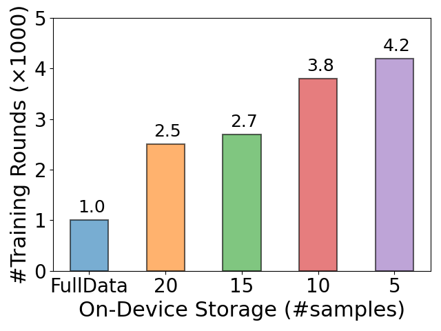
(a) Convergence Time

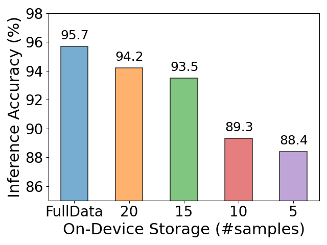
(b) Inference Accuracy

Figure 1. To investigate the impact of on-device storage on FL model training, we conduct experiments on an industrial traffic classification dataset with $30$ mobile devices and $35,000+$ data samples under different storage capacities.

Design Challenges. The design of such an online data selection framework for FL involves three key challenges:

(1) There is still no theoretical understanding about the impact of local on-device data on the training speedup and accuracy enhancement of global model in FL. Lacking information about raw data and local models of the other devices, it is challenging for one device to figure out the impact of its local data sample on the performance of the global model. Furthermore, the sample-level correlation between convergence rate and model accuracy is still not explored in FL, and it is non-trivial to simultaneously improve these two aspects through one unified data valuation metric.

(2) The lack of temporal and spatial information complicates the online data selection in FL. For streaming data, we could not access the data samples coming from the future or discarded in the past. Lacking such temporal information, one device is not able to leverage the complete statistical information (e.g., unbiased local data distribution) for accurate data quality evaluation, such as outliers and noise detection (Shin et al., 2022; Li et al., 2021d). Additionally, due to the distributed paradigm in FL, one device cannot conduct effective data selection without the knowledge of other devices’ stored data and local models, which can be called as spatial information. This is because the valuable data samples selected locally could be overlapped with each other and the local valuable data may not be the global valuable one.

(3) The on-device data selection needs to be low computation-and-memory-cost due to the conflict of limited hardware resources and requirement on quality of user experience. As the additional time delay and memory costs introduced by online data selection process would degrade the performance of mobile network and user experience, the real-time data samples must be evaluated in a computation and memory efficient way. However, increasingly complex ML models lead to high computation complexity as well as large memory footprint for storing intermediate model outputs during the data selection process.

Limitations of Related Works. The prior works on data evaluation and selection in ML failed to solve the above challenges.
(1) The data selection methods in CL, such as leave-one-out test (Cook, 1977), Data Shapley (Ghorbani and Zou, 2019) and Importance Sampling (Mireshghallah et al., 2021; Zhao and Zhang, 2015), are not appropriate for FL due to the first challenge: they could only measure the value of each data sample corresponding to the local model training process, instead of the global model in FL.
(2) The prior works on data selection in FL did not consider the two new properties of FL devices. Mercury (Zeng et al., 2021), FedBalancer (Shin et al., 2022) and the work from Li et al. (Li et al., 2021d) adopted importance sampling framework (Zhao and Zhang, 2015) to select the data samples with high loss or gradient norm but failed to solve the second challenge: these methods all need to inspect the whole dataset for normalized sampling weight computation as well as noise and outliers removal (Hu et al., 2021; Li et al., 2021d).

Our Solutions. To solve the above challenges, we design ODE, an online data selection framework that coordinates networked devices to select and store valuable data samples locally and collaboratively in FL, with theoretical guarantees for accelerating model convergence and enhancing inference accuracy, simultaneously.

In ODE, we first theoretically analyze the impact of an individual local data sample on the convergence rate and final accuracy of the global model in FL. We discover a common dominant term in these two analytical expressions, which can thus be regarded as a reasonable data selection metric in FL. Second, considering the lack of temporal and spatial information, we propose an efficient method for clients to approximate this data selection metric by maintaining a local gradient estimator on each device and a global one on the server. Third, to overcome the potential overlap of the stored data caused by distributed data selection, we further propose a strategy for the server to coordinate each device to store high valuable data from different data distribution regions. Finally, to achieve the computation and memory efficiency, we propose a simplified version of ODE, which replaces the full model gradient with partial model gradient to concurrently reduce the computation and memory costs of the data evaluation process.

System Implementation and Experimental Results. We evaluated ODE on three public tasks: synthetic task (ST) (Caldas et al., 2018), Image Classification (IC) (Xiao et al., 2017) and Human Activity Recognition (HAR) (Ouyang et al., 2021; Li et al., 2021b), as well as one industrial mobile traffic classification dataset (TC) collected from our $30$-days deployment on $30$ ONTs in practice, consisting of $560,000+$ packets from $250$ mobile applications. We compare ODE against three categories of data selection baselines: random sampling (Vitter, 1985), data selection for CL (Shin et al., 2022; Li et al., 2021d; Zeng et al., 2021) and data selection for FL (Shin et al., 2022; Li et al., 2021d). The experimental results show that ODE outperforms all these baselines, achieving as high as $9.52\times$ speedup of model training and $7.56\%$ increase in final model accuracy on ST, $1.35\times$ and $1.4\%$ on IC, $2.22\times$ and $6.38\%$ on HAR, $2.5\times$ and $6\%$ on TC, with low extra time delay and memory costs. We also conduct detailed experiments to analyze the robustness of ODE to various environment factors and its component-wise effect.

Summary of Contributions. (1) To the best of our knowledge, we are the first to identify two new properties of applying FL in mobile networks: limited on-device storage and streaming networked data, and demonstrate its enormity on the effectiveness and efficiency of model training in FL. (2) We provide analytical formulas on the impact of an individual local data sample on the convergence rate and the final inference accuracy of the global model, based on which we propose a new data valuation metric for data selection in FL with theoretical guarantees for accelerating model convergence and improving inference accuracy, simultaneously. Further, we propose ODE, an online data selection framework for FL, to realize the on-device data selection and cross-device collaborative data storage. (3) We conduct extensive experiments on three public datasets and one industrial traffic classification dataset to demonstrate the remarkable advantages of ODE against existing methods.

2. Preliminaries

In this section, we present the learning model and training process of FL. We consider the synchronous FL framework (McMahan et al., 2017; Li et al., 2018; Karimireddy et al., 2020), where a server coordinates a set of mobile devices/clients $C$ to conduct distributed model training. Each client $c\!\in\!C$ generates data samples in a streaming manner with a velocity $v_{c}$. We use $P_{c}$ to denote the client $c$’s underlying distribution of her local data, and $\tilde{P}_{c}$ to represent the empirical distribution of the data samples $B_{c}$ stored in her local storage. The goal of FL is to train a global model $w$ from the locally stored data $\tilde{P}\!=\!\bigcup_{c\in C}\tilde{P}_{c}$ with good performance with respect to the underlying unbiased data distribution ${P}\!=\!\bigcup_{c\in C}P_{c}$:

$$\small\min\limits_{w\in\mathbb{R}^{n}}F(w)=\sum\limits_{c\in C}\zeta_{c}\cdot F_{c}(w),$$

where $\zeta_{c}=\frac{v_{c}}{\sum_{c^{\prime}\!\in\!C}v_{c^{\prime}}}$ denotes the normalized weight of each client, $n$ is the dimension of model parameters, $F_{c}(w)=\mathbb{E}_{(x,y)\sim P_{c}}[l(w,x,y)]$ is the expected loss of the model $w$ over the true data distribution of client $c$. We also use $\tilde{F}_{c}(w)=\frac{1}{|B_{c}|}\sum_{x,y\in B_{c}}l(w,x,y)$ to denote the empirical loss of model over the data samples stored by client $c$.

In this work, we investigate the impacts of each client’s limited storage on FL, and consider the widely adopted algorithm Fed-Avg (McMahan et al., 2017) for easy illustration. Under the synchronous FL framework, the global model is trained by repeating the following two steps for each communication round $t$ from 1 to $T$:

(1) Local Training: In the round $t$, the server selects a client subset $C_{t}\!\subseteq\!C$ to participate in the training process. Each participating client $c\!\in\!C_{t}$ downloads the current global model $w_{\mathrm{fed}}^{t-1}$ (the ending global model in the last round), and performs model updates with the locally stored data for $m$ epochs:

(1) $$\small w_{c}^{t,i}\leftarrow w_{c}^{t,i-1}-\eta\nabla_{w}\tilde{F}_{c}(w_{c}^{t,i-1}),\ i=1,\cdots,m$$

where the starting local model $w_{c}^{t,0}$ is initialized as $w_{\mathrm{fed}}^{t-1}$, and $\eta$ denotes the learning rate.

(2) Model Aggregation: Each participant client $c\!\in\!C_{t}$ uploads the updated local model $w_{c}^{t,m}$, and the server aggregates them to generate a new global model $w_{\mathrm{fed}}^{t}$ by taking a weighted average:

(2) $$\small w_{\mathrm{fed}}^{t}\leftarrow\sum\limits_{c\in C_{t}}\zeta_{c}^{t}\cdot w_{c}^{t,m},$$

where $\zeta_{c}^{t}=\frac{v_{c}}{\sum_{c^{\prime}\in C_{t}}v_{c^{\prime}}}$ is the normalized weight of client $c$.

In the scenario of FL with limited on-device storage and streaming data, we have an additional data selection step for clients:

(3) Data Selection: In each round $t$, once receiving a new data sample, the client has to make an online decision on whether to store the new sample (in place of an old one if the storage area is fully occupied) or discard it. The goal of this data selection process is to select valuable data samples from streaming data for model training in the coming rounds.

3. Design of ODE

In this section, we first quantify the impact of a local data sample on the performance of global model in terms of convergence rate and inference accuracy. Based on the common dominant term in the two analytical expressions, we propose a new data valuation metric for data evaluation and selection in FL (§3.1), and develop a practical method to estimate this metric with low extra computation and communication overhead (§3.2). We further design a strategy for the server to coordinate cross-client data selection process, avoiding the potential overlapped data selected and stored by clients (§3.3). Finally, we summarize the detailed procedure of ODE (§3.4).

3.1. Data Valuation Metric

We evaluate the impact of a local data sample on FL from the perspectives of convergence rate and inference accuracy, which are two critical aspects for the success of FL. The convergence rate quantifies the reduction of loss function in each training round, and determines the communication cost of FL. The inference accuracy reflects the effectiveness of a FL model on guaranteeing the quality of service and user experience. For theoretical analysis, we follow one typical assumption on the FL models, which is widely adopted in the literature (Li et al., 2018; Nguyen et al., 2020; Zhao et al., 2018).

Assumption 1.

(Lipschitz Gradient) For each client $c\!\in\!C$, the loss function $F_{c}(w)$ is $L_{c}$-Lipschitz gradient, i.e., $\parallel\!\nabla_{w}F_{c}(w_{1})-\nabla_{w}F_{c}(w_{2})\!\parallel_{2}\leqslant\!L_{c}\!\parallel\!w_{1}-w_{2}\!\parallel_{2}$, which implies that the global loss function $F(w)$ is $L$-Lipschitz gradient with $L=\sum_{c\in C}\zeta_{c}L_{c}$.

Due to the limitation of space, we provide the proofs of all the theorems and lemmas in our technical report (Gong et al., 2023).

Convergence Rate. We provide a lower bound on the reduction of loss function of global model after model aggregation in each communication round.

Theorem 1.

(Global Loss Reduction) With Assumption 1, for an arbitrary set of clients $C_{t}\!\subseteq\!C$ selected by the server in round $t$, the reduction of global loss $F(w)$ is bounded by:

(3) $$\underbrace{F(w_{\mathrm{fed}}^{t-1})-F(w_{\mathrm{fed}}^{t})}_{\mathrm{global\ loss\ reduction}}\geqslant \sum\limits_{c\in C_{t}}\sum\limits_{i=0}^{m-1}\sum\limits_{(x,y)\in B_{c}}\big{[}-\alpha_{c}\underbrace{\parallel\nabla_{w}l(w_{c}^{t,i},x,y)\parallel_{2}^{2}}_{\mathrm{term}\ 1}$$

$$+\beta_{c}\underbrace{\langle\nabla_{w}l(w_{c}^{t,i},x,y),\nabla_{w}F(w_{\mathrm{fed}}^{t-1})\rangle}_{\mathrm{term}\ 2}\big{]},$$

where $\alpha_{c}=\frac{L}{2\zeta_{c}^{t}}\cdot\left(\frac{\eta}{|B_{c}|}\right)^{2}$ and $\beta_{c}=\zeta_{c}^{t}\cdot\left(\frac{\eta}{|B_{c}|}\right)$.

Due to the different magnitude orders of coefficients $\alpha_{c}$ and $\beta_{c}$ and also the values of terms 1 and 2, as is shown in Appendix B, we can focus on the term $2$ (projection of the local gradient of a data sample onto the global gradient) to evaluate a local data sample’s impact on the convergence rate.

We next briefly describe how to evaluate data samples based on the term 2. The local model parameter $w_{c}^{t,i}$ in term $2$ is computed from (1), where the gradient $\nabla_{w}\tilde{F}_{c}(w_{c}^{t,i-1})$ depends on the “cooperation” of all the stored data samples. Thus, we can formulate the computation of term 2 as a cooperative game (Branzei et al., 2008), where each data sample represents a player and the utility of the whole dataset is the value of term $2$. Within this cooperative game, we can regard the individual contribution of each data sample as its value, and quantify it through leave-one-out (Cook, 1977; Koh and Liang, 2017) or Shapley Value (Ghorbani and Zou, 2019; Shapley, 1953). As these methods require multiple model retraining to compute the marginal contribution of each data sample, we propose a one-step look-ahead strategy to approximately evaluate each sample’s value by only focusing on the first local training epoch ($m=1$).

Inference Accuracy. We can assume that the optimal FL model can be obtained by gathering all clients’ generated data and conducting CL. Moreover, as the accurate testing dataset and the corresponding testing accuracy are hard to obtain in FL, we use the weight divergence between the models trained through FL and CL to quantify the accuracy of the FL model in each round $t$. With $t\!\rightarrow\!\infty$, we can measure the final accuracy of FL model.

Theorem 2.

(Model Weight Divergence) With Assumption 1, for arbitrary set of participating clients $C_{t}$, we have the following inequality for the weight divergence after the $t^{th}$ training round between the models trained through FL and CL.

(4) $$\parallel w_{\mathrm{fed}}^{t}-w_{\mathrm{cen}}^{mt}\parallel_{2}\leqslant (1+\eta L)^{m}\parallel w_{\mathrm{fed}}^{t-1}-w_{\mathrm{cen}}^{m(t-1)}\parallel_{2}$$

$$+\sum\limits_{c\in C_{t}}\zeta_{c}^{t}\left[\eta\sum\limits_{i=0}^{m-1}(1+\eta L)^{m-1-i}G_{c}(w_{c}^{t,i})\right],$$

where $G_{c}(w)=\parallel\nabla_{w}\tilde{F}_{c}(w)-\nabla_{w}F(w)\parallel_{2}$.

The following lemma further shows the impact of a local data sample on $\parallel\!w_{\mathrm{fed}}^{t}-w_{\mathrm{cen}}^{mt}\!\parallel_{2}$ through $G_{c}(w_{c}^{t,i})$.

Lemma 0.

(Gradient Divergence) For an arbitrary client $c\!\in\!C$, $G_{c}(w)\!=\parallel\!\nabla\tilde{F}_{c}(w)-\nabla F(w)\!\parallel_{2}$ is bounded by:

(5) $$G_{c}(w)\!\leqslant\!\sqrt{\delta+\!\sum\limits_{(x,y)\in B_{c}}\frac{1}{|B_{c}|}(\underbrace{\parallel\nabla_{w}l(w,x,y)\parallel_{2}^{2}}_{\mathrm{term\ 1}}-2\underbrace{\langle\nabla_{w}l(w,x,y),\nabla_{w}F(w)\rangle}_{\mathrm{term\ 2}})},$$

where $\delta=\parallel\!\nabla_{w}F(w)\!\parallel_{2}^{2}$ is a constant term for all data samples.

Intuitively, due to different coefficients, the twofold projection (term $2$) has larger mean and variance than the gradient magnitude (term $1$) among different data samples, which is also verified in our experiments in Appendix B. Thus, we can quantify the impact of a local data sample on $G_{c}(w)$ and the inference accuracy mainly through term $2$ in (5), which happens to be the same as the term $2$ in the bound of global loss reduction in (3).

Data Valuation. Based on the above analysis, we define a new data valuation metric in FL, and provide the theoretical understanding as well as intuitive interpretation.

Definition 0.

(Data Valuation Metric) In the $t^{th}$ round, for a client $c\!\in\!C$, the value of a data sample $(x,y)$ is defined as the projection of its local gradient $\nabla l(w,x,y)$ onto the global gradient of the current global model over the unbiased global data distribution:

(6) $$\small v(x,y)\overset{\mathrm{def}}{=}\langle\nabla_{w}l(w_{\mathrm{fed}}^{t},x,y),\nabla_{w}F(w_{\mathrm{fed}}^{t})\rangle.$$

Based on this new data valuation metric, once a client receives a new data sample, she can make an online decision on whether to store this sample by comparing the data value of the new sample with those of old samples in storage, which can be easily implemented as a priority queue.

Theoretical Understanding. On the one hand, maximizing the above data valuation metric of the selected data samples is a one-step greedy strategy for minimizing the loss of the updated global model in each training round according to (3), accelerating model training. On the other hand, this metric also improves the inference accuracy of the final global model by narrowing the gap between the models trained through FL and CL, as it reduces the high-weight term of the dominant part in (4), i.e., $(1+\eta L)^{m-1}G_{c}(w_{k}^{t,0})$.

Intuitive Interpretation. The proposed data valuation metric guides the clients to select the data samples which not only follow their own local data distribution, but also have similar effect with the global data distribution. In this way, the personalized information of local data distribution is preserved and the data heterogeneity across clients is also reduced, which have been demonstrated to improve FL performance (Zawad et al., 2021; Chai et al., 2019; Wang et al., 2020; Yang et al., 2021).

3.2. On-Client Data Selection

In practice, it is non-trivial for one client to directly utilize the above data valuation metric for online data selection due to the following two problems: (1) lack of the latest global model: due to the partial participation of clients in FL (Jhunjhunwala et al., 2022), each client $c\!\in\!C$ does not receive the global FL model $w_{\mathrm{fed}}^{t-1}$ in the rounds that she is not selected, and only has the outdated global FL model from the previous participating round, i.e., $w_{\mathrm{fed}}^{t_{c,\mathrm{last}}-1}$; (2) lack of unbiased global gradient: the accurate global gradient over the unbiased global data distribution can only be obtained by aggregating all the clients’ local gradients over their unbiased local data distributions. This is hard to achieve because only partial clients participate in each communication round, and the locally stored data distribution could become biased during the on-client data selection process.

We can consider that problem (1) does not affect the online data selection process too much as the value of each data sample remains stable across a few training rounds, which is demonstrated with the experiment results in Appendix B, and thus clients can simply use the old global model for data valuation.

To solve the problem (2), we propose a gradient estimation method. First, to solve the issue of skew local gradient, we require each client $c\in C$ to maintain a local gradient estimator $\hat{g}_{c}$, which will be updated whenever the client receives the $n^{th}$ new data sample $(x,y)$ from the last participating round:

(7) $$\small\hat{g}_{c}\leftarrow\frac{n-1}{n}\hat{g_{c}}+\frac{1}{n}\nabla_{w}l(w_{\mathrm{fed}}^{t_{c,\mathrm{last}}-1},x,y).$$

When the client $c$ is selected to participate in FL at a certain round $t$, the client uploads the current local gradient estimator $\hat{g_{c}}$ to the server, and resets the local gradient estimator, i.e., $\hat{g_{c}}\leftarrow 0,n\leftarrow 0$, because a new global FL model $w_{\mathrm{fed}}^{t-1}$ is received. Second, to solve the problem of skew global gradient due to the partial client participation, the server also maintains a global gradient estimator $\hat{g}^{t}$, which is an aggregation of the local gradient estimators, $\hat{g}^{t}=\sum_{c\in C}\zeta_{c}\hat{g}_{c}$. As it would incur high communication cost to collect $\hat{g_{c}}$ from all the clients, the server only uses $\hat{g}_{c}$ of the participating clients to update global gradient estimator $\hat{g}^{t}$ in each round $t$:

(8) $$\small\hat{g}^{t}\leftarrow\hat{g}^{t-1}+\sum_{c\in C_{t}}\zeta_{c}(\hat{g}_{c}-\hat{g}_{c}^{t_{\mathrm{last}}}),$$

Thus, in each training round $t$, the server needs to distribute both the current global FL model $w^{t-1}_{\mathrm{fed}}$ and the latest global gradient estimator $\hat{g}^{t-1}$ to each selected client $c\!\in\!C_{t}$, who will conduct local model training, and upload both locally updated model $w_{c}^{t,m}$ and local gradient estimator $\hat{g_{c}}$ back to the server.

Simplified Version. In both of the local gradient estimation in (7) and data valuation in (6), for a new data sample, we need to backpropagate the entire model to compute its gradient, which will introduce high computation cost and memory footprint for storing intermediate model outputs. To reduce these costs, we only use the gradients of the last few network layers of ML models instead of the whole model, as partial model gradient is also able to reflect the trend of the full gradient, which is also verified in Appendix B.

Privacy Concern. The transmission of local gradient estimators may disclose the local gradient of each client to some extent, which can be avoided by adding Guassian noise to each local gradient estimator before uploading, as in differential privacy (Wei et al., 2020; Dwork, 2008).

3.3. Cross-Client Data Storage

Since the local data distributions of clients may overlap with each other, independently conducting data selection process for each client may lead to distorted global data distribution. One potential solution is to divide the global data distribution into several regions, and coordinate each client to store valuable data samples for one specific distribution region, while the union of all stored data can still follow the unbiased global data distribution. In this work, we consider the label of data samples as the dividing criterion. Thus, before the training process, the server needs to instruct each client the labels and the corresponding quantity of data samples to store. Considering the partial client participation and heterogeneous data distribution among clients, the cross-client coordination strategy need to satisfy the following four desirable properties:

(1) Efficient Data Selection: To improve the efficiency of data selection, the label $y\!\in\!Y$ should be assigned to the clients who generate more data samples with this label, following the intuition that there is a higher probability to select more valuable data samples from a larger pool of candidate data samples.

(2) Redundant Label Assignment: To ensure that all the labels are likely to be covered in each round even with partial client participation, we require each label $y\!\in\!Y$ to be assigned to more than $n^{\mathrm{label}}_{y}$ clients, which is a hyperparameter decided by the server.

(3) Limited Storage: Due to limited on-device storage, each client $c$ should be assigned to less than $n^{\mathrm{client}}_{c}$ labels to ensure a sufficient number of valuable data samples stored for each assigned label, and $n^{\mathrm{client}}_{c}$ is also a hyperparameter decided by the server;

(4) Unbiased Global Distribution: The weighted average of all clients’ stored data distribution is expected to be equal to the unbiased global data distribution, i.e., $\tilde{P}(y)=P(y),\forall y\!\in\!Y$.

We formulate the cross-client data storage with the above four properties by representing the coordination strategy as a matrix $D\!\in\!\mathbb{N}^{|C|\times|Y|}$, where $D_{c,y}$ denotes the number of data samples with label $y$ that client $c$ should store. We use matrix $V\!\in\!\mathbb{R}^{|C|\times|Y|}$ to denote the statistical information of each client’s generated data, where $V_{c,y}\!=\!v_{c}P_{c}(y)$ is the average speed of the data samples with label $y$ generated by client $c$. The cross-client coordination strategy can be obtained by solving the following optimization problem, where the condition (1) is formulated as the objective, and conditions (2), (3), and (4) are described by the constraints (9b), (9c), and (9d), respectively:

(9a) $$\max_{D}\quad \sum\limits_{c\in C}\sum\limits_{y\in Y}D_{c,y}\cdot V_{c,y}=\parallel DV\parallel_{1},$$

(9b) $$\mathrm{s.t.}\quad \parallel D^{\mathrm{T}}_{y}\parallel_{0}\geqslant n^{\mathrm{label}}_{y}, \forall y\!\in\!Y,$$

(9c) $$\parallel D_{c}\parallel_{0}\leqslant n_{c}^{\mathrm{client}}, \forall c\!\in\!C,$$

$$\parallel D_{c}\parallel_{1}=|B_{c}|, \forall c\!\in\!C,$$

(9d) $$\frac{\sum_{c\in C}D_{c,y}}{\parallel B\parallel_{1}}=\frac{\sum_{c\in C}V_{c,y}}{\parallel V\parallel_{1}}, \forall y\!\in\!Y.$$

Complexity Analysis. We can verify that the above optimization problem with $\mathrm{l_{0}}$ norm is a general convex-cardinality problem, which is NP-hard (Natarajan, 1995; Ge et al., 2011). To solve this problem, we divide it into two subproblems: (1) decide which elements of matrix $D$ are non-zero, i.e., $S=\{(c,y)|D_{c,y}\neq 0\}$, that is to assign labels to clients under the constraints of (9b) and (9c); (2) determine the specific values of the non-zero elements of matrix $D$ by solving a simplified convex optimization problem:

(10) $$\max_{D} \sum_{c\in C,y\in Y,(c,y)\in S}D_{c,y}\cdot V_{c,y}$$

$$\mathrm{s.t.} \sum_{y\in Y,(c,y)\in S}D_{c,y}=|B_{c}|, \forall c\!\in\!C,$$

$$\frac{\sum_{c\in C,(c,y)\in S}D_{c,y}}{\parallel D\parallel_{1}}=\frac{\sum_{c\in C}V_{c,y}}{\parallel V\parallel_{1}}, \forall y\!\in\!Y.$$

As the number of possible $S$ can be exponential to $|C|$ and $|Y|$, it is still prohibitively expensive to derive the globally optimal solution of $D$ with large $|C|$ (massive clients in FL). The classic approach is to replace the non-convex discontinuous $l_{0}$ norm constraints with the convex continuous $l_{1}$ norm regularization terms in the objective function (Ge et al., 2011), which fails to work in our scenario because simultaneously minimizing as many as $|C|+|Y|$ non-differentiable $l_{1}$ norm in the objective function will lead to high computation and memory costs as well as unstable solutions (Schmidt et al., 2007; Shi et al., 2010). Thus, we propose a greedy strategy to solve this complicated problem.

Greedy Cross-Client Coordination Strategy. We achieve the four desirable properties through the following three steps:

(1) Information Collection: Each client $c\!\in\!C$ sends the rough information about local data to the server, including the storage capacity $|B_{c}|$ and data velocity $V_{c,y}$ of each label $y$, which can be obtained from the statistics of previous time periods. Then, the server can construct the vector of storage size $B\!\in\!\mathbb{N}^{|C|}$ and the matrix of data velocity $V\!\in\!\mathbb{R}^{|C|\times|Y|}$ of all clients.

(2) Label Assignment: The server sorts labels according to a non-decreasing order of the total number of clients having this label. We prioritize the labels with top rank in label-client assignment, because these labels are more difficult to find enough clients to meet Redundant Label Assignment property. For each considered label $y\!\in\!Y$ in the rank, there could be multiple clients to be assigned, and the server allocates label $y$ to clients $c$ who generates data samples with label $y$ in a higher data velocity. By doing this, we attempt to satisfy the property of Efficient Data Selection. Once the number of labels assigned to client $c$ is larger than $n_{c}^{\mathrm{client}}$, this client will be removed from the rank due to the Limited Storage property.

(3) Quantity Assignment: With the above two steps, we have decided the non-zero elements of the client-label matrix $D$, i.e., the set $S$. To further reduce the computational complexity and avoid the imbalanced on-device data storage for each label, we do not directly solve the simplified optimization problem in (10). Instead, we require each client to divide the storage capacity evenly to the assigned labels, and compute a weight $\gamma_{y}$ for each label $y\!\in\!Y$ to guarantee that the weighted distribution of the stored data approximates the unbiased global data distribution, i.e., satisfying $\gamma_{y}\tilde{P}(y)\!=\!P(y)$. Accordingly, we can derive the weight $\gamma_{y}$ for each label $y$ by setting

(11) $$\small\gamma_{y}=\frac{P(y)}{\tilde{P}(y)}=\frac{\parallel V^{\mathrm{T}}_{y}\parallel_{1}/\parallel V\parallel_{1}}{\parallel D^{\mathrm{T}}_{y}\parallel_{1}/\parallel D\parallel_{1}}.$$

Thus, each client $c$ only needs to maintain one priority queue with a size $\frac{|B_{c}|}{\parallel D_{c}\parallel_{0}}$ for each assigned label. In the local model training, each participating client $c\!\in\!C_{t}$ updates the local model using the weighted stored data samples:

(12) $$\small w_{c}^{t,i}\leftarrow w_{c}^{t,i-1}-\frac{\eta}{\zeta_{c}}\sum_{(x,y)\in B_{c}}\gamma_{y}\nabla_{w}l(w_{c}^{t,i-1},x,y),$$

where $\zeta_{c}\!=\!\sum_{(x,y)\in B_{c}}\gamma_{y}$ denotes the new weight of each client, and the normalized weight of client $c\!\in\!C_{t}$ for model aggregation in round $t$ becomes $\zeta_{c}^{t}=\sum_{c\!\in\!C_{t}}\frac{\zeta_{c}}{\sum_{c^{\prime}\!\in\!C_{t}}\zeta_{c^{\prime}}}$.

We illustrate a simple example in Appendix A for better understanding of the above procedure.

Privacy Concern. The potential privacy leakage of uploading rough local information is tolerable in practice, and can be further avoided through Homomorphic Encryption (Acar et al., 2018), which enables to sort $k$ encrypted data samples with complexity $O(k\log k^{2})$ (Hong et al., 2021).

3.4. Overall Procedure of ODE

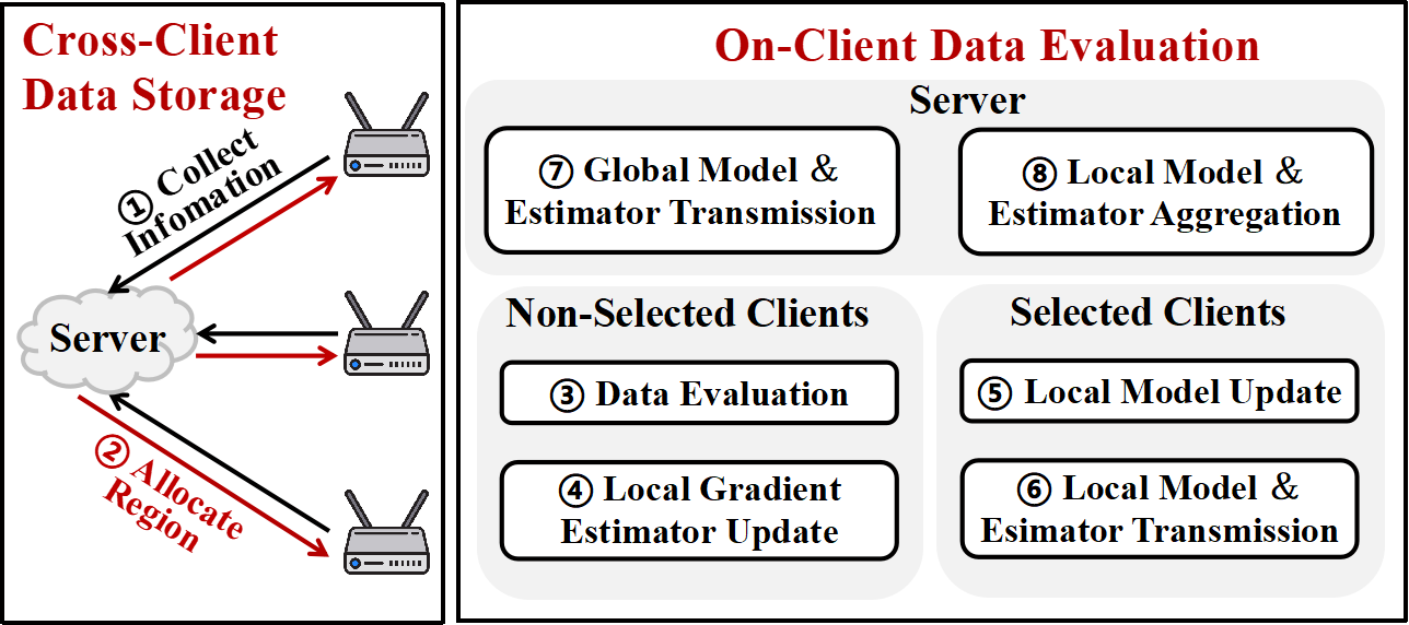
Figure 2. Overview of ODE framework.

Overview of ODE framework.

ODE incorporates cross-client data storage and on-client data evaluation to coordinate mobile devices to store valuable samples, speeding up model training process and improving inference accuracy of the final model. The overall procedure is shown in Figure 2.

Key Idea. Intuitively, the cross-client data storage component coordinates clients to store the high-quality data samples with different labels to avoid highly overlapped data stored by all clients. And the on-client data evaluation component instructs each client to select the data having similar gradient with the global data distribution, which reduces the data heterogeneity among clients while also preserves personalized information.

Cross-Client Data Storage. Before the FL process, the central server collects data distribution information and storage capacity from all clients (①), and solving the optimization problem in (9) through our greedy approach (②).

On-Client Data Evaluation. During the FL process, clients train the local model in participating rounds, and utilize idle computation and memory resources to conduct on-device data selection in non-participating rounds. In the $t^{th}$ training round, non-selected clients, selected clients and the server perform different operations:

$\bullet\$Non-selected clients: Data Evaluation (③): each non-selected client $c\!\in\!C\setminus C_{t}$ continuously evaluates and selects the data samples according to the data valuation metric in (6), within which the clients use the estimated global gradient received in last participation round instead of the accurate global one. Local Gradient Estimator Update (④): the client also continuously updates the local gradient estimator $\hat{g}_{c}$ using (7).

$\bullet\$Selected Clients: Local Model Update (⑤): after receiving the new global model $w_{\mathrm{fed}}^{t-1}$ and new global gradient estimator $\hat{g}^{t-1}$ from the server, each selected client $c\!\in\!C_{t}$ performs local model updates using the stored data samples by (12). Local Model and Estimator Transmission (⑥): each selected client sends the updated model $w_{c}^{t,m}$ and local gradient estimator $\hat{g}_{c}$ to the server. The local estimator $\hat{g}_{c}$ will be reset to $0$ for approximating local gradient of the newly received global model $w_{\mathrm{fed}}^{t-1}$.

$\bullet\$ Server: Global Model and Estimator Transmission (⑦): At the beginning of each training round, the server distributes the global model $w_{\mathrm{fed}}^{t-1}$ and the global gradient estimator $\hat{g}^{t-1}$ to the selected clients. Local Model and Estimator Aggregation (⑧): at the end of each training round, the server collects the updated local models $w_{c}^{t,m}$ and local gradient estimators $\hat{g}_{c}$ from participating clients $c\!\in\!C_{t}$, which will be aggregated to obtain a new global model by (2) and a new global gradient estimator by (8).

4. Evaluation

In this section, we first introduce experiment setting, baselines and evaluation metrics. Second, we present the overall performance of ODE and baselines on model training speedup and inference accuracy improvement, as well as the memory footprint and evaluation delay. Next, we show the robustness of ODE against various environment factors. We also show the individual and integrated impacts of limited storage and streaming data on FL to show our motivation, and analyze the individual effect of different components of ODE, which are shown in Appendix C.4 and C.5 due to the limited space.

4.1. Experiment Setting

Tasks, Datasets and ML Models. To demonstrate the ODE’s good performance and generalization across various tasks, datasets and ML models. we evaluate ODE on one synthetic dataset, two real-world datasets and one industrial dataset, all of which vary in data quantities, distributions and model outputs, and cover the tasks of Synthetic Task (ST), Image Classification (IC), Human Activity Recognition (HAR) and mobile Traffic Classification (TC). The statistics of the tasks are summarized in Table 6, and introduced in details in Appendix C.1.

Tasks	Datasets	Models	$\#$Samples	$\#$Labels	$\#$Devices	$n_{y}^{\mathrm{label}}$	$\frac{|C_{t}|}{|C|}$	$\eta$	$m$	$|B_{c}|$
ST	Synthetic Dataset (Caldas et al., 2018)	LogReg	$1,016,442$	$10$	$200$	$5$	$5\%$	$1e^{-4}$	$5$	$10$
IC	Fashion-MNIST (Xiao et al., 2017)	LeNet (LeCun et al., 1989)	$70,000$	$10$	$50$	$5$	$10\%$	$1e^{-3}$	$5$	$5$
HAR	HARBOX (Ouyang et al., 2021)	Customized DNN	$34,115$	$5$	$120$	$5$	$10\%$	$1e^{-3}$	$5$	$5$
TC	Industrial Dataset	Customized CNN	$37,853$	$20$	$30$	$5$	$20\%$	$5e^{-3}$	$5$	$10$

Table 1. Information of different tasks, datasets, models and default experiment settings.

Parameters Configurations. The main configurations are shown in Table 6 and other configurations like the training optimizer and velocity of on-device data stream are presented in Appendix C.2.

Baselines. In our experiments, we compare two versions of ODE, ODE-Exact (using exact global gradient) and ODE-Est (using estimated global gradient), with four categories of data selection methods, including random sampling methods (RS), importance-sampling based methods for CL (HL and GN), previous data selection methods for FL (FB and SLD) and the ideal case with unlimited on-device storage (FD). These methods are introduced in details in Appendix C.3.

Metrics for Training Performance. We use two metrics to evaluate the performance of each method: (1) Time-to-Accuracy Ratio: we measure the training speedup of global model by the ratio of training time of RS and the considered method to reach the same target accuracy, which is set to be the final inference accuracy of RS. As the time of one communication round is usually fixed in practical FL scenario, we can quantify the training time with the number of communicating rounds. (2) Final Inference Accuracy: we evaluate the inference accuracy of the final global model on each device’s testing data and report the average accuracy for evaluation.

4.2. Overall Performance

We compare the performance of ODE with four baselines on all the datasets, and show the results in Table 2.

Task	Model Training Speedup
	RS	HL	GN	FB	SLD	ODE-Exact	ODE-Est	FD
ST	$1.0\times$	$-$	$4.87\times$	$-$	$4.08\times$	$9.52\times$	$5.88\times$	$2.67\times$
IC	$1.0\times$	$-$	$-$	$-$	$-$	$1.35\times$	$1.20\times$	$1.01\times$
HAR	$1.0\times$	$-$	$-$	$-$	$-$	$2.22\times$	$1.55\times$	$4.76\times$
TC	$1.0\times$	$-$	$-$	$-$	$-$	$2.51\times$	$2.50\times$	$3.92\times$
Task	Inference Accuracy
ST	$79.56\%$	$78.44\%$	$83.28\%$	$78.56\%$	$82.38\%$	$87.12\%$	$82.80\%$	$88.14\%$
IC	$71.31\%$	$51.95\%$	$41.45\%$	$60.43\%$	$69.15\%$	$72.71\%$	$72.70\%$	$71.37\%$
HAR	$67.25\%$	$48.16\%$	$51.02\%$	$48.33\%$	$56.24\%$	$73.63\%$	$70.39\%$	$77.54\%$
TC	$89.3\%$	$69.00\%$	$69.3\%$	$72.19\%$	$72.30\%$	$95.3\%$	$95.30\%$	$96.00\%$

Table 2. ODE’s improvements on model training speedup and inference accuracy. The symbol ’$-$’ means that the method fails to reach the target accuracy.

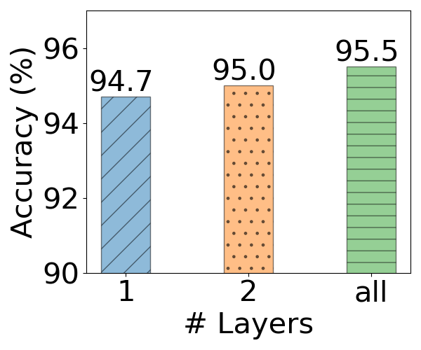
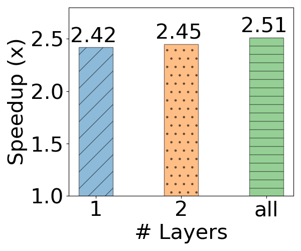
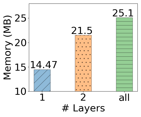
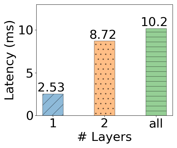
Figure 3. Performance and cost of simplified ODE with different $\#$model layers.

Performance and cost of simplified ODE with different $\#$model layers.

ODE significantly speeds up the model training process. We observed that ODE improves time-to-accuracy performance over the existing data selection methods on all the four datasets. Compared with baselines, ODE achieves the target accuracy $5.88\times\!\!\sim\!\!9.52\times$ faster on ST; $1.20\times\!\!\sim\!\!1.35\times$ faster on IC; $1.55\times\!\!\sim\!\!2.22\times$ faster on HAR; $2.5\times$ faster on TC. Also, we observe that the largest speedup is achieved on the datast ST, because the high non-i.i.d degree across clients and large data divergence within clients leave a great potential for ODE to reduce data heterogeneity and improve training process through data selection.

ODE largely improves the final inference accuracy. Table 2 shows that in comparison with baselines with the same storage, ODE enhances final accuracy on all the datasets, achieving $3.24\%\!\!\sim\!\!7.56\%$ higher on ST, $3.13\%\!\!\sim\!\!6.38\%$ increase on HAR, and around $6\%$ rise on TC. We also notice that ODE has a marginal accuracy improvement ($\approx\!1.4\%$) on IC, because the FashionMNIST has less data variance within each label, and a randomly selected subset is sufficient to represent the entire data distribution for model training.

Importance-based data selection methods perform poorly. Table 2 shows that these methods even cannot reach the target final accuracy on tasks IC, HAR and TC, as these datasets are collected from real world and contain noise data, making such importance sampling methods fail to work (Shin et al., 2022; Li et al., 2021d).

Previous data selection methods for FL outperform importance based methods but worse than ODE. As is shown in Table 2, FedBalancer and SLD perform better than HL and GN, but worse than RS in a large degree, which is different from the phenomenon in traditional settings (Katharopoulos and Fleuret, 2018; Li et al., 2021d; Shin et al., 2022). This is because (1) their noise reduction steps, such as removing samples with top loss or gradient norm, highly rely on the complete statistical information of full dataset, and (2) their on-client data valuation metrics fail to work for the global model training in FL, as discussed in §1.

Simplified ODE reduces computation and memory costs significantly with little performance degradation. We conduct another two experiments which consider only the last 1 and 2 layers (5 layers in total) for data valuation on the industrial TC dataset. Empirical results shown in Figure 3 demonstrate that the simplified version reduces as high as $44\%$ memory and $83\%$ time delay, with only $1\%$ and $0.1\times$ degradation on accuracy and speedup.

ODE introduces small extra memory footprint and data processing delay during data selection process.

Task	Memory Footprint (MB)
	RS	HL	GN	ODE-Est	ODE-Simplified
IC	1.70	11.91	16.89	18.27	16.92
HAR	1.92	7.27	12.23	13.46	12.38
TC	0.75	10.58	19.65	25.15	14.47
Task	Evaluation Time (ms)
IC	0.05	11.1	21.1	22.8	11.4
HAR	0.05	0.36	1.04	1.93	0.53
TC	0.05	1.03	9.06	9.69	1.23

Table 3. The memory footprint and evaluation delay per sample valuation of baselines on three real-world tasks.

Empirical results in Table 3 demonstrate that simplified ODE brings only tiny evaluation delay and memory burden to mobile devices ($1.23$ms and $14.47$MB for TC task), and thus can be applied to practical network scenario.

4.3. Robustness of ODE

In this subsection, we mainly compare the robustness of ODE and previous methods to various factors in industrial environments, such as the number of local training epoch $m$, client participation rate $\frac{|C_{t}|}{|C|}$, storage capacity $|B_{c}|$, mini-batch size and data heterogeneity across clients, on the industrial TC dataset.

Number of Local Training Epoch. Empirical results shown in Figure 4(b) demonstrate that ODE can work with various local training epoch numbers $m$. With $m$ increasing, both of ODE-Exact and ODE-Est achieve higher final inference accuracy than existing methods with same setting.

Participation Rate. The results in Figure 5(b) demonstrate that ODE can improve the FL process significantly even with small participation rate, accelerating the model training $2.57\times$ and increasing the inference accuracy by $6.6\%$. This demonstrates the practicality of ODE in the industrial environment, where only a small proportion of mobile devices could be ready to participate in each FL round.

Other Factors. We also demonstrate the remarkable robustness of ODE to device storage capacity, mini-batch size and data heterogeneity across clients compared with previous methods, which are fully presented in the technical report (Gong et al., 2023).

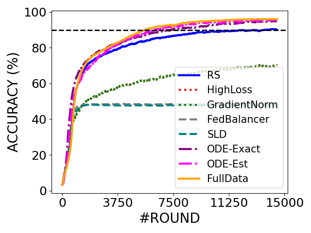
(a) Epoch=2

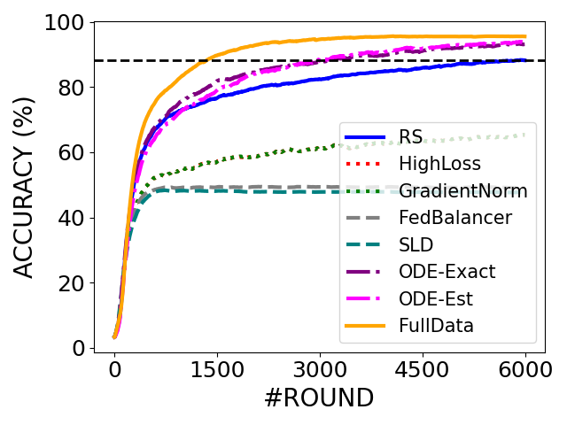
(b) Epoch=10

Figure 4. The training process of different sampling methods with various numbers of local epoch.

The training process of different sampling methods with various numbers of local epoch.

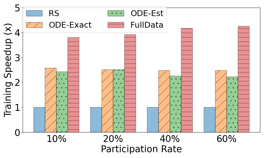
(a) Training Speedup

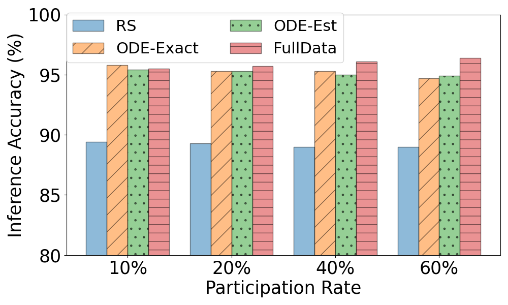
(b) Final Accuracy

Figure 5. The performance of different data selection methods with various participation rates.

The performance of different data selection methods with various participation rates.

5. Related Works

Federated Learning is a distributed learning framework that aims to collaboratively learn a global model over the networked devices’ data under the constraint that the data is stored and processed locally (Li et al., 2020; McMahan et al., 2017). Existing works mostly focus on how to overcome the data heterogeneity problem (Chai et al., 2019; Zawad et al., 2021; Cho et al., 2022a; Wolfrath et al., 2022), reduce the communication cost (Khodadadian et al., 2022, 2022; Hou et al., 2021; Yang et al., 2020), select important clients (Cho et al., 2022b; Nishio and Yonetani, 2019; Li et al., 2021c; Li et al., 2021a) or train a personalized model for each client (Wu et al., 2021; Fallah et al., 2020). Despite that a few works consider the problem of online and continuous FL (Wang et al., 2022; Chen et al., 2020; Yoon et al., 2021), they did not consider the device properties of limited on-device storage and streaming networked data.

Data Selection. In FL, selecting data from streaming data can be seen as sampling batches of data from its distribution, which is similar to mini-batch SGD. To improve the training process of SGD, existing methods quantify the importance of each data sample (such as loss (Shrivastava et al., 2016; Schaul et al., 2015), gradient norm (Johnson and Guestrin, 2018; Zhao and Zhang, 2015), uncertainty (Chang et al., 2017; Wu et al., 2017), data shapley (Ghorbani and Zou, 2019) and representativeness (Mirzasoleiman et al., 2020; Wang et al., 2021)) and leverage importance sampling or priority queue to select training samples. The previous literature (Shin et al., 2022; Li et al., 2021d) on data selection in FL simplify conducts the above data selection methods on each client individually for local model training without considering the global model. And all of them require either access to all the data or multiple inspections over the data stream, which are not satisfied in the mobile network scenarios.

6. Conclusion

In this work, we identify two key properties of networked FL: limited on-device storage and streaming networked data, which have not been fully explored in the literature. Then, we present the design, implementation and evaluation of ODE, which is an online data selection framework for FL with limited on-device storage, consisting of two components: on-device data evaluation and cross-device collaborative data storage. Our analysis show that ODE improves both convergence rate and inference accuracy of the global model, simultaneously. Empirical results on three public and one industrial datasets demonstrate that ODE significantly outperforms the state-of-the-art data selection methods in terms of training time, final accuracy and robustness to various factors in industrial environments.

Appendix A Simple Example

In Figure 6, We use a simple example to illustrate our proposed greedy solution for the cross-device collaborative data selection described in §3.3.

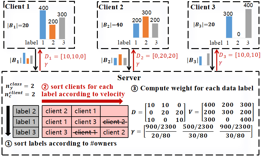
Figure 6. A simple example to illustrate the greedy coordination. ① Sort labels according to $\#$owners and obtain label order $\{2,1,3\}$; ② Sort and allocate clients for each label under the constraint of $n_{c}^{\mathrm{client}}$ and $n_{y}^{\mathrm{class}}$; ③ Obtain coordination matrix $D$ and compute class weight $\gamma$ according to (11).

A simple example to illustrate the greedy coordination. ① Sort labels according to $\#$owners and obtain label order $\{2,1,3\}$; ② Sort and allocate clients for each label under the constraint of $n_{c}^{\mathrm{client}}$ and $n_{y}^{\mathrm{class}}$; ③ Obtain coordination matrix $D$ and compute class weight $\gamma$ according to (11).

Appendix B Empirical results for claims.

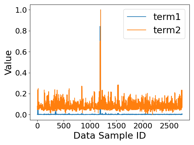
(a) Term 1 vs Term 2

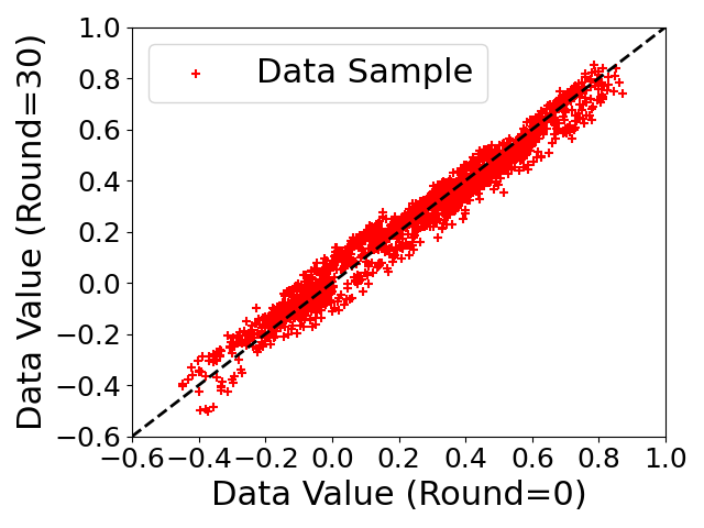
(b) Round 0 vs Round 30

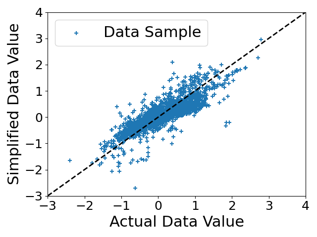
(c) Full model vs Last layer

Figure 7. Empirical results to support some claims, and the experiment setting could be found in §4.1. (a): comparison of the normalized values of two terms in (3) and (5). (b): comparison of the data values computed in round 0 and round 30. (c): comparison of the data values computed using gradients of full model layers and the last layer.

Empirical results to support some claims, and the experiment setting could be found in §4.1. (a): comparison of the normalized values of two terms in (3) and (5). (b): comparison of the data values computed in round 0 and round 30. (c): comparison of the data values computed using gradients of full model layers and the last layer.

Empirical results to support some claims mentioned before, and the experiment setting could be found in §4.1. Figure 7(a): comparison of the normalized values of two terms in (3) and (5). Figure 7(b): comparison of the data values computed in round 0 and round 30. Figure 7(c): comparison of the data values computed using gradients of full model layers and the last layer.

Appendix C Experiments

C.1. Tasks and Datasets

Synthetic Task. The synthetic dataset we used is proposed in LEAF benchmark (Caldas et al., 2018) and is also described in details in (Li et al., 2018). It contains $200$ clients and 1 million data samples, and a Logistic Regression model is trained for this 10-class task.

Image Classification. Fashion-MNIST (Xiao et al., 2017) contains $60,000$ training images and $10,000$ testing images, which are divided into 50 clients according to labels (McMahan et al., 2017). We train LeNet (LeCun et al., 1989) for the 10-class image classification.

Human Activity Recognition. HARBOX (Ouyang et al., 2021) is the 9-axis OMU dataset collected from 121 users’ smartphones in a crowdsourcing manner, including 34,115 data samples with $900$ dimension. Considering the simplicity of the dataset and task, a lightweight customized DNN with two dense layers followed by a SoftMax layer is deployed for this 5-class human activity recognition task (Li et al., 2022).

Traffic Classification. The industrial dataset about the task of mobile application classification is collected by our deployment of $30$ ONTs (optimal network terminal) in a simulated network environment from May 2019 to June 2019. Generally, the dataset contains more than $560,000$ data samples and has more than $250$ applications as labels, which cover the application categories of videos (such as YouTube and TikTok), games (such as LOL and WOW), files downloading (such as AppStore and Thunder) and communication (such as WhatsApp and WeChat). We manually label the application of each data sample. The model we applied is a CNN consisting of 4 convolutional layers with kernel size $1\times 3$ to extract features and 2 fully-connected layers for classification, which is able to achieve $95\%$ accuracy through CL and satisfy the on-device resource requirement due to the small number of model parameters. To reduce the training time caused by the large scale of dataset, we randomly select $20$ out of $250$ applications as labels with various numbers of data samples, whose distribution is shown in Figure 9.

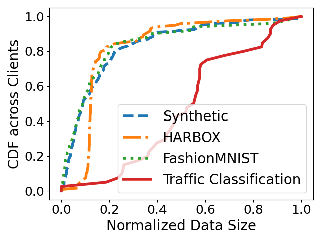
Figure 8. Unbalanced data quantity of clients.

Unbalanced data quantity of clients.

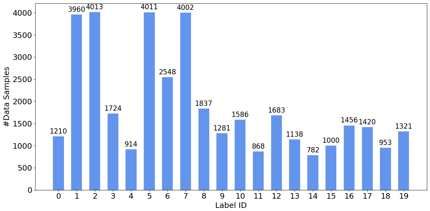
Figure 9. Data distribution in traffic classification dataset.

Data distribution in traffic classification dataset.

C.2. Configurations

For all the experiments, we use SGD as the optimizer and decay the learning rate per $100$ rounds by $\eta_{\mathrm{new}}=0.95\times\eta_{\mathrm{old}}$. To simulate the setting of streaming data, we set the on-device data velocity to be $v_{c}=\frac{\#\mathrm{training\ samples}}{500}$, which means that each device $c\!\in\!C$ will receive $v_{c}$ data samples one by one in each communication round, and the samples would be shuffled and appear again per $500$ rounds. Other default configurations are shown in Table 6. Note that the participating clients in each round are randomly selected, and for each experiment, we repeat $5$ times and show the average results.

C.3. Baselines

(1) Random sampling methods including RS (Reservoir Sampling (Vitter, 1985)) and FIFO (First-In-First-Out: storing the latest $|B_{c}|$ data samples).

(2) Importance sampling-based methods including HighLoss (HL), using the loss of each data sample as data value to reflect the informativeness of data (Loshchilov and Hutter, 2015; Shrivastava et al., 2016; Schaul et al., 2015), and GradientNorm (GN), quantifying the impact of each data sample on model update through its gradient norm (Johnson and Guestrin, 2018; Zhao and Zhang, 2015).

(3) Previous data selection methods for canonical FL including FedBalancer (FB) (Shin et al., 2022) and SLD (Sample-Level Data selection) (Li et al., 2021d) which are revised slightly to adapt to streaming data setting: (i) We store the loss/gradient norm of the latest $50$ samples for noise removal; (ii) For FedBalancer, we ignore the data samples with loss larger than top $10\%$ loss value, and for SLD, we remove the samples with gradient norm larger than the median norm value.

(4) Ideal case with unlimited on-device storage, denoted as FullData (FD), using the entire dataset of each client for training to simulate the unlimited storage scenario,.

C.4. Motivating Experiments

In this section, We provide the complete experimental evidences for our motivation. First, we prove that the properties of limited on-device storage and streaming data can deteriorate the classic FL model training process significantly in various settings, such as different numbers of local training epochs and different data heterogeneity among clients. Then, we analyze the separate impact of theses two properties on FL with different data selection methods. Due to limited space, we only provide the main conclusions here and the details of the experiment settings and results are provided in the technical report (Gong et al., 2023).

The main results are: (1) When the number of local epoch $m$ increases, the negative impact of limited on-device storage is becoming more serious due to larger steps towards the biased update direction, slowing down the convergence time $3.92\times$ and decreasing the final model accuracy by as high as $6.7\%$; (2) With the variance of local data increasing, the reduction of convergence rate and model accuracy is becoming larger. This is because the stored data samples are more likely to be biased due to wide data distribution; (3) The property of streaming data prevents previous methods from making accurate online decisions, as they select each sample according to a normalized probability depending on both discarded and upcoming samples, which are not available in streaming setting. But ODE selects each data sample through a deterministic valuation metric, not affected by the other samples; (4) The property of limited storage is the essential failure of existing data selection methods as it prevents previous methods from obtaining full local and global data information, guiding clients to select suboptimal data from an insufficient candidate dataset. In contrast, ODE allows clients to select valuable samples with global information from server.

C.5. Component-wise Analysis

In this subsection, we evaluate the effectiveness of each of the three components in ODE: on-device data selection, global gradient estimator and cross-client coordination strategy. The detailed experimental settings, results and analysis are presented in the technical report (Gong et al., 2023), and we only present the main conclusions here.

On-Client Data Selection. The result shows that without data valuation module, Valuation- performs slightly better than RS but much worse than ODE-Est, which demonstrates the significant role of our data valuation and selection metric.

Global Gradient Estimator. Experimental results show that using the naive estimation method instead of our proposed local and global gradient estimators will lead to really poor performance, as the partial client participation and biased local gradient will cause the inaccurate estimation for global gradient, which further misleads the clients to select samples using a wrong valuation metric.

Cross-Client Coordination. Empirical result shows that without the cross-client coordination component, the performance of ODE is largely weakened, as the clients tend to store similar and overlapped valuable data samples and the other data will be under-represented.

The results altogether show that each component is critical for the good performance of ODE.

Appendix D Proofs

The full proofs of theorems and lemmas are also provided in the technical report (Gong et al., 2023) due to limited space.

References

- (1)
- Acar et al. (2018) Abbas Acar, Hidayet Aksu, A Selcuk Uluagac, and Mauro Conti. 2018. A survey on homomorphic encryption schemes: Theory and implementation. Comput. Surveys 51, 4 (2018), 1–35.
- Aggarwal et al. (2021) Puneet Kumar Aggarwal, Parita Jain, Jaya Mehta, Riya Garg, Kshirja Makar, and Poorvi Chaudhary. 2021. Machine learning, data mining, and big data analytics for 5G-enabled IoT. In Blockchain for 5G-Enabled IoT. 351–375.
- Akbari et al. (2021) Iman Akbari, Mohammad A Salahuddin, Leni Ven, Noura Limam, Raouf Boutaba, Bertrand Mathieu, Stephanie Moteau, and Stephane Tuffin. 2021. A look behind the curtain: traffic classification in an increasingly encrypted web. Proceedings of the ACM on Measurement and Analysis of Computing Systems 5, 1 (2021), 1–26.
- Arora et al. (2016) Deepali Arora, Kin Fun Li, and Alex Loffler. 2016. Big data analytics for classification of network enabled devices. In International Conference on Advanced Information Networking and Applications Workshops (WAINA).
- Ayoubi et al. (2018) Sara Ayoubi, Noura Limam, Mohammad A Salahuddin, Nashid Shahriar, Raouf Boutaba, Felipe Estrada-Solano, and Oscar M Caicedo. 2018. Machine learning for cognitive network management. IEEE Communications Magazine 56, 1 (2018), 158–165.
- Banchs et al. (2021) Albert Banchs, Marco Fiore, Andres Garcia-Saavedra, and Marco Gramaglia. 2021. Network intelligence in 6G: challenges and opportunities. In ACM Workshop on Mobility in the Evolving Internet Architecture (MobiArch).
- Bega et al. (2019) Dario Bega, Marco Gramaglia, Marco Fiore, Albert Banchs, and Xavier Costa-Perez. 2019. DeepCog: Optimizing resource provisioning in network slicing with AI-based capacity forecasting. IEEE Journal on Selected Areas in Communications 38, 2 (2019), 361–376.
- Bhuyan et al. (2013) Monowar H Bhuyan, Dhruba Kumar Bhattacharyya, and Jugal K Kalita. 2013. Network anomaly detection: methods, systems and tools. IEEE Communications Surveys & Tutorials 16, 1 (2013), 303–336.
- Branzei et al. (2008) Rodica Branzei, Dinko Dimitrov, and Stef Tijs. 2008. Models in cooperative game theory. Vol. 556. Springer Science & Business Media.
- Caldas et al. (2018) Sebastian Caldas, Sai Meher Karthik Duddu, Peter Wu, Tian Li, Jakub Konečnỳ, H Brendan McMahan, Virginia Smith, and Ameet Talwalkar. 2018. Leaf: A benchmark for federated settings. arXiv preprint arXiv:1812.01097 (2018).
- Chai et al. (2019) Zheng Chai, Hannan Fayyaz, Zeshan Fayyaz, Ali Anwar, Yi Zhou, Nathalie Baracaldo, Heiko Ludwig, and Yue Cheng. 2019. Towards taming the resource and data heterogeneity in federated learning. In USENIX Conference on Operational Machine Learning (OpML).
- Chang et al. (2017) Haw-Shiuan Chang, Erik Learned-Miller, and Andrew McCallum. 2017. Active bias: Training more accurate neural networks by emphasizing high variance samples. In Conference on Neural Information Processing Systems (NeurIPS).
- Chen et al. (2020) Yujing Chen, Yue Ning, Martin Slawski, and Huzefa Rangwala. 2020. Asynchronous online federated learning for edge devices with non-iid data. In IEEE International Conference on Big Data (BigData).
- Cho et al. (2022a) Yae Jee Cho, Andre Manoel, Gauri Joshi, Robert Sim, and Dimitrios Dimitriadis. 2022a. Heterogeneous Ensemble Knowledge Transfer for Training Large Models in Federated Learning. In International Joint Conferences on Artificial Intelligence Organization (IJCAI).
- Cho et al. (2022b) Yae Jee Cho, Jianyu Wang, and Gauri Joshi. 2022b. Towards understanding biased client selection in federated learning. In International Conference on Artificial Intelligence and Statistics (AISTATS).
- Cook (1977) R Dennis Cook. 1977. Detection of influential observation in linear regression. Technometrics 19, 1 (1977), 15–18.
- Cruz (1995) Rene L. Cruz. 1995. Quality of service guarantees in virtual circuit switched networks. IEEE Journal on Selected areas in Communications 13, 6 (1995), 1048–1056.
- Deng (2019) Yunbin Deng. 2019. Deep learning on mobile devices: a review. In Mobile Multimedia/Image Processing, Security, and Applications.
- Dwork (2008) Cynthia Dwork. 2008. Differential privacy: A survey of results. In International Conference on Theory and Applications of Models of Computation (ICTAMC).
- Fallah et al. (2020) Alireza Fallah, Aryan Mokhtari, and Asuman Ozdaglar. 2020. Personalized federated learning with theoretical guarantees: A model-agnostic meta-learning approach. Conference on Neural Information Processing Systems (NeurIPS.
- Ge et al. (2011) Dongdong Ge, Xiaoye Jiang, and Yinyu Ye. 2011. A note on the complexity of L p minimization. Mathematical Programming 129, 2 (2011), 285–299.
- Ghorbani and Zou (2019) Amirata Ghorbani and James Zou. 2019. Data shapley: Equitable valuation of data for machine learning. In International Conference on Machine Learning (ICML).
- Giordani et al. (2020) Marco Giordani, Michele Polese, Marco Mezzavilla, Sundeep Rangan, and Michele Zorzi. 2020. Toward 6G networks: Use cases and technologies. IEEE Communications Magazine 58, 3 (2020), 55–61.
- Gong et al. (2023) Chen Gong, Zhenzhe Zheng, Fan Wu, Bingshuai Li, Yunfeng Shao, and Guihai Chen. 2023. To Store or Not? Online Data Selection for Federated Learning with Limited Storage. https://drive.google.com/file/d/10PpbxDgqnAaokDtHg_WeW4O7RS49FGOd/view?usp=share_link
- Hamer et al. (2020) Jenny Hamer, Mehryar Mohri, and Ananda Theertha Suresh. 2020. Fedboost: A communication-efficient algorithm for federated learning. In International Conference on Machine Learning (ICML).
- Hong et al. (2021) Seungwan Hong, Seunghong Kim, Jiheon Choi, Younho Lee, and Jung Hee Cheon. 2021. Efficient sorting of homomorphic encrypted data with k-way sorting network. IEEE Transactions on Information Forensics and Security 16 (2021), 4389–4404.
- Hou et al. (2021) Charlie Hou, Kiran Koshy Thekumparampil, Giulia Fanti, and Sewoong Oh. 2021. FedChain: Chained Algorithms for Near-optimal Communication Cost in Federated Learning. In International Conference on Learning Representations (ICLR).
- Hu et al. (2021) Niel Teng Hu, Xinyu Hu, Rosanne Liu, Sara Hooker, and Jason Yosinski. 2021. When does loss-based prioritization fail? ICML 2021 workshop on Subset Selection in ML (2021).
- Jhunjhunwala et al. (2022) Divyansh Jhunjhunwala, PRANAY SHARMA, Aushim Nagarkatti, and Gauri Joshi. 2022. FedVARP: Tackling the Variance Due to Partial Client Participation in Federated Learning. In Conference on Uncertainty in Artificial Intelligence (UAI).
- Johnson and Guestrin (2018) Tyler B Johnson and Carlos Guestrin. 2018. Training deep models faster with robust, approximate importance sampling. Conference on Neural Information Processing Systems (NeurIPS).
- Karimireddy et al. (2020) Sai Praneeth Karimireddy, Satyen Kale, Mehryar Mohri, Sashank Reddi, Sebastian Stich, and Ananda Theertha Suresh. 2020. Scaffold: Stochastic controlled averaging for federated learning. In International Conference on Machine Learning (ICML).
- Katharopoulos and Fleuret (2018) Angelos Katharopoulos and François Fleuret. 2018. Not all samples are created equal: Deep learning with importance sampling. In International conference on machine learning (ICML).
- Khodadadian et al. (2022) Sajad Khodadadian, Pranay Sharma, Gauri Joshi, and Siva Theja Maguluri. 2022. Federated Reinforcement Learning: Linear Speedup Under Markovian Sampling. In International Conference on Machine Learning (ICML).
- Koh and Liang (2017) Pang Wei Koh and Percy Liang. 2017. Understanding black-box predictions via influence functions. In International Conference on Machine Learning (ICML).
- Kolahi et al. (2011) Samad S Kolahi, Shaneel Narayan, Du DT Nguyen, and Yonathan Sunarto. 2011. Performance monitoring of various network traffic generators. In International Conference on Computer Modelling and Simulation (UkSim).
- Krishna and Murty (1999) K Krishna and M Narasimha Murty. 1999. Genetic K-means algorithm. IEEE Transactions on Systems, Man, and Cybernetics 29, 3 (1999), 433–439.
- LeCun et al. (1989) Yann LeCun, Bernhard Boser, John Denker, Donnie Henderson, Richard Howard, Wayne Hubbard, and Lawrence Jackel. 1989. Handwritten digit recognition with a back-propagation network. In Conference on Neural Information Processing Systems (NeurIPS), Vol. 2.
- Li et al. (2021c) Ang Li, Jingwei Sun, Pengcheng Li, Yu Pu, Hai Li, and Yiran Chen. 2021c. Hermes: an efficient federated learning framework for heterogeneous mobile clients. In International Conference On Mobile Computing And Networking (MobiCom).
- Li et al. (2021d) Anran Li, Lan Zhang, Juntao Tan, Yaxuan Qin, Junhao Wang, and Xiang-Yang Li. 2021d. Sample-level Data Selection for Federated Learning. In IEEE International Conference on Computer Communications (INFOCOM).
- Li et al. (2021b) Chenglin Li, Di Niu, Bei Jiang, Xiao Zuo, and Jianming Yang. 2021b. Meta-har: Federated representation learning for human activity recognition. In The ACM Web Conference (WWW).
- Li et al. (2022) Chenning Li, Xiao Zeng, Mi Zhang, and Zhichao Cao. 2022. PyramidFL: A Fine-grained Client Selection Framework for Efficient Federated Learning. In International Conference On Mobile Computing And Networking (MobiCom).
- Li et al. (2021a) Fengjiao Li, Jia Liu, and Bo Ji. 2021a. Federated learning with fair worker selection: A multi-round submodular maximization approach. In IEEE International Conference on Mobile Ad-Hoc and Smart Systems (MASS). 180–188.
- Li et al. (2020) Tian Li, Anit Kumar Sahu, Ameet Talwalkar, and Virginia Smith. 2020. Federated learning: Challenges, methods, and future directions. IEEE Signal Processing Magazine 37, 3 (2020), 50–60.
- Li et al. (2018) Tian Li, Anit Kumar Sahu, Manzil Zaheer, Maziar Sanjabi, Ameet Talwalkar, and Virginia Smith. 2018. Federated optimization in heterogeneous networks. In Proceedings of Machine Learning and Systems (MLSys).
- Loshchilov and Hutter (2015) Ilya Loshchilov and Frank Hutter. 2015. Online batch selection for faster training of neural networks. arXiv preprint arXiv:1511.06343 (2015).
- McMahan et al. (2017) Brendan McMahan, Eider Moore, Daniel Ramage, Seth Hampson, and Blaise Aguera y Arcas. 2017. Communication-efficient learning of deep networks from decentralized data. In International Conference on Artificial Intelligence and Statistics (AISTATS).
- Mireshghallah et al. (2021) Fatemehsadat Mireshghallah, Mohammadkazem Taram, Ali Jalali, Ahmed Taha Taha Elthakeb, Dean Tullsen, and Hadi Esmaeilzadeh. 2021. Not all features are equal: Discovering essential features for preserving prediction privacy. In The ACM Web Conference (WWW).
- Mirzasoleiman et al. (2020) Baharan Mirzasoleiman, Jeff Bilmes, and Jure Leskovec. 2020. Coresets for data-efficient training of machine learning models. In International Conference on Machine Learning (ICML).
- Murtagh and Contreras (2012) Fionn Murtagh and Pedro Contreras. 2012. Algorithms for hierarchical clustering: an overview. Wiley Interdisciplinary Reviews: Data Mining and Knowledge Discovery 2, 1 (2012), 86–97.
- Natarajan (1995) Balas Kausik Natarajan. 1995. Sparse approximate solutions to linear systems. SIAM J. Comput. 24, 2 (1995), 227–234.
- Nguyen et al. (2020) Hung T Nguyen, Vikash Sehwag, Seyyedali Hosseinalipour, Christopher G Brinton, Mung Chiang, and H Vincent Poor. 2020. Fast-convergent federated learning. IEEE Journal on Selected Areas in Communications 39, 1 (2020), 201–218.
- Nishio and Yonetani (2019) Takayuki Nishio and Ryo Yonetani. 2019. Client selection for federated learning with heterogeneous resources in mobile edge. In IEEE International Conference on Communications (ICC).
- Nunes et al. (2015) David Sousa Nunes, Pei Zhang, and Jorge Sá Silva. 2015. A survey on human-in-the-loop applications towards an internet of all. IEEE Communications Surveys & Tutorials 17, 2 (2015), 944–965.
- Ouyang et al. (2021) Xiaomin Ouyang, Zhiyuan Xie, Jiayu Zhou, Jianwei Huang, and Guoliang Xing. 2021. ClusterFL: a similarity-aware federated learning system for human activity recognition. In ACM International Conference on Mobile Systems, Applications, and Services (MobiSys).
- Rafique and Velasco (2018) Danish Rafique and Luis Velasco. 2018. Machine learning for network automation: overview, architecture, and applications. Journal of Optical Communications and Networking 10, 10 (2018), D126–D143.
- Schaul et al. (2015) Tom Schaul, John Quan, Ioannis Antonoglou, and David Silver. 2015. Prioritized experience replay. In International Conference on Learning Representations (ICLR).
- Schmidt et al. (2007) Mark Schmidt, Glenn Fung, and Rmer Rosales. 2007. Fast optimization methods for l1 regularization: A comparative study and two new approaches. In European Conference on Machine Learning (ECML).
- Shapley (1953) L Shapley. 1953. Quota solutions op n-person games1. Edited by Emil Artin and Marston Morse (1953), 343.
- Shi et al. (2010) Jianing Shi, Wotao Yin, Stanley Osher, and Paul Sajda. 2010. A fast hybrid algorithm for large-scale l1-regularized logistic regression. The Journal of Machine Learning Research 11 (2010), 713–741.
- Shin et al. (2022) Jaemin Shin, Yuanchun Li, Yunxin Liu, and Sung-Ju Lee. 2022. FedBalancer: data and pace control for efficient federated learning on heterogeneous clients. In ACM International Conference on Mobile Systems, Applications, and Services (MobiSys). 436–449.
- Shrivastava et al. (2016) Abhinav Shrivastava, Abhinav Gupta, and Ross Girshick. 2016. Training region-based object detectors with online hard example mining. In The IEEE / CVF Computer Vision and Pattern Recognition Conference (CVPR).
- Siddiqi et al. (2019) Murtaza Ahmed Siddiqi, Heejung Yu, and Jingon Joung. 2019. 5G ultra-reliable low-latency communication implementation challenges and operational issues with IoT devices. Electronics 8, 9 (2019), 981.
- Tahaei et al. (2020) Hamid Tahaei, Firdaus Afifi, Adeleh Asemi, Faiz Zaki, and Nor Badrul Anuar. 2020. The rise of traffic classification in IoT networks: A survey. Journal of Network and Computer Applications 154 (2020), 102538.
- UCSC (2020) UCSC. 2020. Packet Buffers. https://people.ucsc.edu/~warner/buffer.html
- Vitter (1985) Jeffrey S Vitter. 1985. Random sampling with a reservoir. ACM Trans. Math. Software 11, 1 (1985), 37–57.
- Wang et al. (2022) Junxiao Wang, Song Guo, Xin Xie, and Heng Qi. 2022. Federated unlearning via class-discriminative pruning. In The ACM Web Conference (WWW).
- Wang et al. (2020) Jianyu Wang, Qinghua Liu, Hao Liang, Gauri Joshi, and H Vincent Poor. 2020. Tackling the objective inconsistency problem in heterogeneous federated optimization. In Advances in neural information processing systems.
- Wang et al. (2021) Yanhao Wang, Francesco Fabbri, and Michael Mathioudakis. 2021. Fair and representative subset selection from data streams. In The ACM Web Conference (WWW).
- Wei et al. (2020) Kang Wei, Jun Li, Ming Ding, Chuan Ma, Howard H Yang, Farhad Farokhi, Shi Jin, Tony QS Quek, and H Vincent Poor. 2020. Federated learning with differential privacy: Algorithms and performance analysis. IEEE Transactions on Information Forensics and Security 15 (2020), 3454–3469.
- Wolfrath et al. (2022) Joel Wolfrath, Nikhil Sreekumar, Dhruv Kumar, Yuanli Wang, and Abhishek Chandra. 2022. HACCS: Heterogeneity-Aware Clustered Client Selection for Accelerated Federated Learning. In IEEE International Parallel & Distributed Processing Symposium (IPDPS).
- Wu et al. (2017) Chao-Yuan Wu, R Manmatha, Alexander J Smola, and Philipp Krahenbuhl. 2017. Sampling matters in deep embedding learning. In The IEEE / CVF Computer Vision and Pattern Recognition Conference (CVPR).
- Wu et al. (2021) Jinze Wu, Qi Liu, Zhenya Huang, Yuting Ning, Hao Wang, Enhong Chen, Jinfeng Yi, and Bowen Zhou. 2021. Hierarchical personalized federated learning for user modeling. In The ACM Web Conference (WWW).
- Xiao et al. (2017) Han Xiao, Kashif Rasul, and Roland Vollgraf. 2017. Fashion-MNIST: a Novel Image Dataset for Benchmarking Machine Learning Algorithms. arXiv:cs.LG/1708.07747 [cs.LG]
- Yang et al. (2021) Chengxu Yang, Qipeng Wang, Mengwei Xu, Zhenpeng Chen, Kaigui Bian, Yunxin Liu, and Xuanzhe Liu. 2021. Characterizing impacts of heterogeneity in federated learning upon large-scale smartphone data. In The ACM Web Conference (WWW).
- Yang et al. (2020) Kai Yang, Tao Jiang, Yuanming Shi, and Zhi Ding. 2020. Federated learning via over-the-air computation. IEEE Transactions on Wireless Communications 19, 3 (2020), 2022–2035.
- Yoon et al. (2021) Jaehong Yoon, Wonyong Jeong, Giwoong Lee, Eunho Yang, and Sung Ju Hwang. 2021. Federated continual learning with weighted inter-client transfer. In International Conference on Machine Learning (ICML).
- Zawad et al. (2021) Syed Zawad, Ahsan Ali, Pin-Yu Chen, Ali Anwar, Yi Zhou, Nathalie Baracaldo, Yuan Tian, and Feng Yan. 2021. Curse or redemption? how data heterogeneity affects the robustness of federated learning. In The AAAI Conference on Artificial Intelligence (AAAI).
- Zeng et al. (2021) Xiao Zeng, Ming Yan, and Mi Zhang. 2021. Mercury: Efficient On-Device Distributed DNN Training via Stochastic Importance Sampling. In ACM Conference on Embedded Networked Sensor Systems (Sensys).
- Zhao and Zhang (2015) Peilin Zhao and Tong Zhang. 2015. Stochastic optimization with importance sampling for regularized loss minimization. In International Conference on Machine Learning (ICML).
- Zhao et al. (2018) Yue Zhao, Meng Li, Liangzhen Lai, Naveen Suda, Damon Civin, and Vikas Chandra. 2018. Federated learning with non-iid data. arXiv preprint arXiv:1806.00582 (2018).