Periodic and solitary waves generating in optical fiber amplifiers and fiber lasers with distributed parameters

Abstract

We study self-similar dynamics of picosecond light pulses generating in optical fiber amplifiers and fiber lasers with distributed parameters. A rich variety of periodic and solitary wave solutions are derived for the governing generalized nonlinear Schrödinger equation with varying coefficients in the presence of gain effect. The constraint on distributed optical fiber parameters for the existence of these wave solutions is presented. The dynamical behaviour of those self-similar waves is discussed in a periodic distributed amplification system. The stability of periodic and solitary wave solutions is also studied numerically by adding white noise. It is proved by using the numerical split-step Fourier method that the profile of these nonlinear self-similar waves remains unchanged during evolution.

I Introduction

A self-similar wave (or a similariton) is a nonlinear wave or a pulse that maintains the same shape during propagation, even though its width and amplitude change according to the management of system parameters Serkin ; Zhang . Particularly, the self-similar structure of a soliton hints that a simple amplification is sufficient to reshape it to the original structure instead of regenerating it Kodama . Within this context, the first experimental observation of beam profile reshaping due to light-induced change of refractive index has been reported in Moll . Moreover, the self-similar evolution of ultrashort parabolic pulses in a laser resonator was also experimentally observed Ilday . In addition, self-similarity has been demonstrated in the evolution of self-written waveguides Kewitsch ; Monro , in the growth of Hill gratings An , and in optical fibers Anderson . These discoveries prove the richness of self-similar behaviours in field of nonlinear optics.

Nowadays, studying the formation and properties of self-similar structures has become an increasingly active field of research R1 -R6 , due to their importance to understand widely various physical phenomena Barenblatt . Notably, these chirped self-similar pulses provide a potential application to the design of fiber optic amplifiers, optical pulse compressors, and solitary wave-based communication links K1 ; D1 ; M1 .

A realistic description of self-similar pulse dynamics in an inhomogeneous Kerr medium is most often based on the generalized nonlinear Schrödinger (NLS) equation with distributed coefficients K1 ; K2 . The various parameters involved in this model which depict group velocity dispersion, cubic nonlinearity, and gain or loss are allowed to change with the propagation distance, thus reflecting the presence of inhomogeneity in the real system. With the inclusion of these varying coefficients, the underlying model becomes difficult to solve exactly. The development of powerful methods for obtaining analytical self-similar solutions and ongoing improvement in the analysis required to determine optical nonlinear waves possessing physically relevant properties are thus essential for studying the self-similar dynamics at both picosecond and femtosecond time scales. For the purpose of identifying different nonlinear waves that may propagate in optical fiber amplifiers and fiber lasers, the self-similarity technique proposed by Kruglov et al. K1 ; K2 ; K3 has been widely used as a powerful method to study the existence of self-similar solutions. We note that thanks to this method, the determination of self-similar wave solutions for the generalized NLS equation with distributed coefficients K1 ; K2 and its many relevant variants R1 ; R2 ; Dai1 ; Dai2 has become possible. For all these studies, the resulting solitary pulse solutions are shown to exhibit special properties such as enhanced linearity in pulse frequency chirp, self-similarity in pulse shape, and stability with respect to finite perturbations. These self-similar wave solutions may be profitably exploited in designing the optimal waveguiding system experiments and further understanding of their transmission properties.

It is of interest to construct other new analytical self-similar solutions to the generalized NLS equation with varied coefficients. No doubt, this can help one to understand the transmission process and hence designing new optical systems and devices. It is also very interesting to develop other self-similarity techniques which can be applicable efficiently to search for more nonlinear waves that can propagate self-similarly in an optical fiber amplifier. Finding new types of self-similar propagating pulses and constructing powerful methods able to solve the generalized NLS equation that describes ultrashort pulse propagation phenomena in a variety of physical situations is an interesting work. In this paper, we have developed a new direct self-similarity method to construct a diversity of new analytical self-similar solutions for the generalized NLS equation that takes distributed second order dispersion, cubic nonlinearity and gain into account. This method also allowed us to determine the self-similar variables and formation conditions of these structures.

The structure of this paper is as follows. In Sec. II, the generalized NLS equation modelling the evolution of picosecond optical pulses in the fiber amplifiers and fiber lasers with distributed parameters in presence of gain effects is presented. The set of nonlinear differential equations that governs the dynamics of wave amplitude in the system is also derived here. Then, in Sec. III, we present the general self-similar form of exact periodic wave solutions and discuss the propagation properties and formation conditions of their existence. In Sec. IV, we have obtained a set of periodical and solitary self-similar waves governed by this generalized NLS equation with distributed coefficients. In Sec. V, we investigate the dynamical behaviour of the self-similar waves in a periodic distributed amplification system for different choices of parameters. We also analyze in Sec. VI the stability of nonlinear wave solutions by numerical simulation. Finally, the results are summarized in Sec. VII.

II Scaling transformation of NLS equation

The picosecond pulses generating in an optical amplifier with distributed parameters are described by the following generalized NLS equation K1 ; K2 ; Serkin1 ; Wang ,

$$i\frac{\partial\psi}{\partial z}=\alpha(z)\frac{\partial^{2}\psi}{\partial\tau^{2}}-\gamma(z)\left|\psi\right|^{2}\psi+\frac{i}{2}g(z)\psi,$$ (1)

where $\psi(z,\tau)$ is the complex field envelope. The variable $z$ represents the distance along direction of propagation and $\tau=t-\int_{0}^{z}\beta_{1}(z^{\prime})dz^{\prime}$ is the time in a moving reference frame where $\beta_{1}(z)$ is the first order distributed dispersion. It means that we made the transformation of time $t$ to new variable $\tau$ (retarded time) which allow to subtract the first order partial time-derivative in the generalized NLS equation. The real distributed parameter $\alpha(z)$ is given as $\alpha(z)=\beta_{2}(z)/2$ where $\beta_{2}(z)$ is the second order dispersion, and the parameters $\gamma(z)$ and $g(z)$ define the nonlinearity and gain effects. Note that the fiber laser can be described by the same NLS equation with additional equations defining the pumping process, feedback effect and appropriate boundary conditions which depend on the model of laser.

It is valuable the following transformation of the wave function $\psi(z,\tau)$ as

$$\psi(z,\tau)=\chi(\zeta,\tau),~{}~{}~{}~{}\frac{d\zeta}{dz}=\alpha(z),$$ (2)

where $\zeta=f(z)$. Thus, the function $f(z)$ is given by

$$\zeta=f(z)=\int_{0}^{z}\alpha(z^{\prime})dz^{\prime},$$ (3)

where is used the boundary condition $f(0)=0$. The generalized NLS equation (1) for new wave function $\chi(\zeta,\tau)$ has the form,

$$i\frac{\partial\chi}{\partial\zeta}=\frac{\partial^{2}\chi}{\partial\tau^{2}}-\tilde{\gamma}(z)\left|\chi\right|^{2}\chi+\frac{i}{2}\tilde{g}(z)\chi.$$ (4)

In this NLS model equation the distributed parameters $\tilde{\gamma}(z)$ and $\tilde{g}(z)$ are given as

$$\tilde{\gamma}(z)=\frac{\gamma(z)}{\alpha(z)},~{}~{}~{}~{}\tilde{g}(z)=\frac{g(z)}{\alpha(z)}.$$ (5)

The traveling wave solutions of the generalized NLS equation (4) have the form,

$$\chi(\zeta,\tau)=A(\zeta)U(\xi)\exp[i(\kappa\zeta-\delta\tau+\theta)],$$ (6)

where $U(\xi)$ is a real amplitude function which depends on the variable $\xi=\tau-q\zeta$, and the parameter $q$ is connected with the inverse velocity of the pulses in retarded frame. The parameter $q$ and modified wave number $\kappa$ depending on the frequency shift $\delta$ are found below. We emphasis that this (modified) wave number is introduced under the variable $\zeta$ which is connected to the distance $z$ by Eq. (3). Thus, the variable $\zeta$ and modified wave number $\kappa$ have not the standard dimensions.

It follows from Eq. (6) that without loss of generality we can use here the boundary condition $A(0)=1$ for the real function $A(\zeta)$. The real parameters $\theta$ represents the phase of pulse at $\zeta=0$. The generalized NLS equation (4) with the wave function $\chi(\zeta,\tau)$ given in Eq. (6) yields the ordinary differential equations for the functions $A(\zeta)$ and $U(\xi)$ as

$$\frac{1}{A(\zeta)}\frac{dA(\zeta)}{d\zeta}=\frac{1}{2}\tilde{g}(z),$$ (7)

$$\frac{d^{2}U}{d\xi^{2}}-\sigma U-\tilde{\gamma}(z)A^{2}(\zeta)U^{3}=0,$$ (8)

where the parameters $\sigma$ and $q$ are given by

$$\sigma=\delta^{2}-\kappa,~{}~{}~{}~{}q=2\delta.$$ (9)

We note that Eq. (8) yields the following constraint $\tilde{\gamma}(z)A^{2}(\zeta)=\mathrm{const}$ because the function $U$ depends on the variable $\xi$. Thus, using the boundary condition $A(0)=1$ we can write this constraint as

$$\frac{\gamma(z)}{\alpha(z)}A^{2}(\zeta)=\frac{\gamma_{0}}{\alpha_{0}},$$ (10)

where $\gamma_{0}=\gamma(0)$, $\alpha_{0}=\alpha(0)$ and $\zeta=f(z)$. Hence, in this case Eq. (8) transforms to the following ordinary nonlinear differential equation,

$$\frac{d^{2}U}{d\xi^{2}}-\sigma U-\frac{\gamma_{0}}{\alpha_{0}}U^{3}=0.~{}~{}~{}~{}~{}~{}$$ (11)

We use also the following definition:

$$A(f(z))\equiv B(z)~{}~{}~{}~{}B(z)=\left(\frac{\gamma_{0}\alpha(z)}{\alpha_{0}\gamma(z)}\right)^{1/2}.$$ (12)

Thus, Eq. (7) can be written in the form,

$$\frac{d\ln B(z)}{dz}=\frac{1}{2}g(z).$$ (13)

III Self-similar form of wave solutions

The equations derived in previous section lead to self-similar wave solutions of general NLS equation (1) with distributed coefficients. Using Eqs. (2), (6) and (12) we can write the wave function of Eq. (1) as

$$\psi(z,\tau)=B(z)U(\xi)\exp[i(\kappa f(z)-\delta\tau+\theta)],$$ (14)

where the variables $\xi$ is

$$\xi=\tau-2\delta f(z),~{}~{}~{}~{}f(z)=\int_{0}^{z}\alpha(z^{\prime})dz^{\prime}.$$ (15)

The integration of Eq. (11) yields the first order nonlinear differential equations for the function $U(\xi)$ as

$$\left(\frac{dU}{d\xi}\right)^{2}=\nu+\sigma U^{2}+\lambda U^{4},$$ (16)

where $\nu$ is the integration constant, and the parameters $\sigma$ and $\lambda$ are given by

$$\sigma=\delta^{2}-\kappa,~{}~{}~{}~{}\lambda=\frac{\gamma_{0}}{2\alpha_{0}}.$$ (17)

We emphasis that $\sigma$ is an arbitrary parameter here because the modified wave number $\kappa$ is not fixed even for given frequency shift $\delta$.

We transform Eq. (16) to new function $F(\xi)$ using relation as

$$U^{2}(\xi)=-\frac{1}{4\lambda}F(\xi).~{}~{}~{}~{}~{}~{}~{}$$ (18)

Thus, we have the nonlinear differential equation for function $F$ as

$$\left(\frac{dF}{d\xi}\right)^{2}=\rho F+\mu F^{2}-F^{3},~{}~{}~{}~{}~{}~{}~{}$$ (19)

where the coefficients $\rho$ and $\mu$ are

$$\rho=-16\nu\lambda,~{}~{}~{}~{}\mu=4\sigma.$$ (20)

Note that in Sec. IV we find the solutions of Eqs. (16) and (19) for particular values of integration constant $\nu$. However, the parameter $\sigma$ is free under some intervals which depend on the particular solution of Eqs. (16) and (19). Hence, the parameter $\mu$ is free as well.

The integration of Eq. (13) with the boundary condition $B(0)=1$ (see Eq. (12)) yields

$$B(z)=\exp\left(\frac{1}{2}\int_{0}^{z}g(z^{\prime})dz^{\prime}\right).$$ (21)

Hence, the nonlinearity coefficient $\gamma(z)$ is given by Eq. (12) as

$$\gamma(z)=\frac{\gamma_{0}}{\alpha_{0}}\alpha(z)\exp\left(-\int_{0}^{z}g(z^{\prime})dz^{\prime}\right).$$ (22)

Let us for an example define the gain as $g(z)=g_{0}=\mathrm{const}$ then the amplitude $B(z)$ and nonlinearity parameter $\gamma(z)$ are

$$B(z)=\exp\left(\frac{1}{2}g_{0}z\right),~{}~{}~{}~{}\gamma(z)=\frac{\gamma_{0}}{\alpha_{0}}\alpha(z)\exp\left(-g_{0}z\right).$$ (23)

One can also consider the amplitude $B(z)$ as an arbitrary function in the class of real increasing functions. In this case the gain $g(z)$ is given by Eq. (13) and the nonlinearity coefficient $\gamma(z)$ follows by constraint in Eq. (10). Let us define the amplitude as $B(z)=1+az$ with $a>0$ then we have

$$g(z)=\frac{2a}{1+az},~{}~{}~{}~{}\gamma(z)=\frac{\gamma_{0}}{\alpha_{0}}\frac{\alpha(z)}{(1+az)^{2}}.$$ (24)

In the following section, we show the existence of a rich set of periodical and solitary waves governed by Eq. (1).

IV Periodic and solitary wave solutions

In this section we present a set of periodic and solitary self-similar wave solutions based on results obtained in Sec. III. The notations for variable $\xi$ and real amplitude $B(z)$ are presented in Eqs. (15) and (21) respectively. The modified wave number $\kappa$ and the variable $\zeta$ are given as

$$\kappa=-\sigma+\delta^{2},~{}~{}~{}~{}\zeta=f(z),$$ (25)

where $\sigma$ and $\delta$ are free parameters and the function $f(z)$ is defined in Eq. (15). However, the frequency shift $\delta$ in quasi-monochromatic approximation should satisfy the condition $\left|\delta\right|/\omega_{0}\ll 1$ where $\omega_{0}$ is the carrier frequency.

Thus, using the above results we have obtained a set of periodical and solitary self-similar waves governed by generalized NLS equation (1). We emphasis that presented periodical solutions depend on three free parameters as the modulus $k$ of Jacobi elliptic functions and free parameters $\sigma$ and $\delta$. The solitary wave solutions presented below depend on two free parameters as $\sigma$ and $\delta$. However, all these solutions depend also on two additional (trivial) free parameters as $\xi_{0}$ and the phase $\theta$. In these wave solutions the parameter $\lambda$ is given by Eq. (17) as $\lambda=\gamma(0)/\beta_{2}(0)$.

1. Periodic waves for $\lambda<0$ and $\sigma>0$

In the case when parameters of wave solution belong the intervals $\lambda<0$ and $\sigma>0$ we have found that Eqs. (16) and (19) yield the periodic solution as

$$U(\xi)=\pm[A+B\mathrm{cn^{2}}(w(\xi-\xi_{0}),k)]^{1/2},~{}~{}~{}~{}~{}~{}~{}$$ (26)

where the modulus $k$ of Jacobi elliptic function $\mathrm{cn}(w(\xi-\xi_{0}),k)$ is given in the interval $0<k<1$. The free parameter (integration constant) $\nu$ in Eqs. (16) and (19) is given by

$$\nu=\frac{\sigma^{2}(1-k^{2})}{\lambda(2-k^{2})^{2}}.$$ (27)

The parameters of periodic solution in Eq. (26) are

$$A=\frac{\sigma(k^{2}-1)}{\lambda(2-k^{2})},~{}~{}~{}~{}B=-\frac{\sigma k^{2}}{\lambda(2-k^{2})},~{}~{}~{}~{}~{}~{}~{}$$ (28)

$$w=\sqrt{\frac{\sigma}{2-k^{2}}}.~{}~{}~{}~{}~{}~{}~{}$$ (29)

It follows from this solution the conditions for parameters as $\sigma>0$ and $\lambda<0$. Substitution of solution (26) into the wave function (14) yields the family of periodic wave solutions for the NLS equation (1) as

$$\psi(z,\tau)=\pm B(z)[A+B\mathrm{cn^{2}}(w(\xi-\xi_{0}),k)]^{1/2}\exp[i(\kappa f(z)-\delta\tau+\theta)],$$ (30)

where $\kappa=-\sigma+\delta^{2}$ and the modulus $k$ is an arbitrary parameter in the interval $0<k<1$ and $\xi_{0}$ is an arbitrary real constant. We note that in the limiting cases with $k=1$ this periodic wave reduces to a bright-type soliton solution.

2. Periodic waves for $\lambda<0$, $\sigma<0$ and $\lambda<0$, $\sigma>0$

In the case when parameters of wave solution belong the intervals $\lambda<0$, $\sigma<0$ and $\lambda<0$, $\sigma>0$ we have found that Eqs. (16) and (19) yield the periodic solution as

$$U(\xi)=\pm\Lambda\mathrm{cn}(w(\xi-\xi_{0}),k),$$ (31)

where $k$ is the modulus of Jacobi elliptic function $\mathrm{cn}(w(\xi-\xi_{0}),k)$. In this case the free parameter (integration constant) $\nu$ in Eqs. (16) and (19) is given by

$$\nu=\frac{\sigma^{2}k^{2}(k^{2}-1)}{\lambda(2k^{2}-1)^{2}}.$$ (32)

The parameters $\Lambda$ and $w$ are given as

$$\Lambda=\sqrt{\frac{-\sigma k^{2}}{\lambda(2k^{2}-1)}},~{}~{}~{}~{}w=\sqrt{\frac{\sigma}{2k^{2}-1}}.$$ (33)

In this solution the modulus $k$ can belong two different intervals: $0<k<1/\sqrt{2}$ or $1/\sqrt{2}<k<1$. It follows from this solution the conditions for parameters as $\lambda<0$ and $\sigma<0$ when $0<k<1/\sqrt{2}$, and the conditions for parameters are $\lambda<0$ and $\sigma>0$ when $1/\sqrt{2}<k<1$. Substitution of the solution (31) into the wave function (14) yields the following family of periodic wave solutions for the generalized NLS equation (1):

$$\psi(z,\tau)=\pm\Lambda B(z)\mathrm{cn}(w(\xi-\xi_{0}),k)\exp[i(\kappa f(z)-\delta\tau+\theta)],$$ (34)

where $\kappa=-\sigma+\delta^{2}$ and the modulus $k$ is an arbitrary parameter in the interval $0<k<1/\sqrt{2}$ or $1/\sqrt{2}<k<1$. In the limiting case with $k=1$ this solution reduces to soliton solution.

3. Periodic waves for $\lambda>0$ and $\sigma<0$

In the case when parameters of wave solution belong the intervals $\lambda>0$ and $\sigma<0$ we have found that Eqs. (16) and (19) yield the periodic solution as

$$U(\xi)=\pm\Lambda\mathrm{sn}(w(\xi-\xi_{0}),k),$$ (35)

where $0<k<1$. Here $\mathrm{sn}(w(\xi-\xi_{0}),k)$ is the Jacobi elliptic function with modulus $k$. In this case the free parameter (integration constant) $\nu$ in Eqs. (16) and (19) is given by

$$\nu=\frac{\sigma^{2}k^{2}}{\lambda(1+k^{2})^{2}}.$$ (36)

The parameters $\Lambda$ and $w$ are given by

$$\Lambda=\sqrt{\frac{-\sigma k^{2}}{\lambda(1+k^{2})}},~{}~{}~{}~{}w=\sqrt{\frac{-\sigma}{1+k^{2}}}.$$ (37)

It follows from this solution the conditions for parameters as $\lambda>0$ and $\sigma<0$. Substitution of the solution (35) into the wave function (14) yields the following family of periodic wave solutions for the generalized NLS equation (1):

$$\psi(z,\tau)=\pm\Lambda B(z)\mathrm{sn}(w(\xi-\xi_{0}),k)\exp[i(\kappa f(z)-\delta\tau+\theta)],$$ (38)

where $\kappa=-\sigma+\delta^{2}$ and the modulus $k$ is an arbitrary parameter in the interval $0<k<1$. In the limiting case with $k=1$ this solution reduces to the kink wave solution.

4. Periodic rational-elliptic waves for $\lambda>0$ and $\sigma<0$

In the case when parameters of wave solution belong the intervals $\lambda>0$ and $\sigma<0$ we have found that Eqs. (16) and (19) yield also the periodic rational-elliptic solution as

$$U(\xi)=\pm\frac{A\mathrm{sn}\left(w(\xi-\xi_{0}),k\right)}{1+\mathrm{dn}\left(w(\xi-\xi_{0}),k\right)},$$ (39)

where $0<k<1$, and the parameter (integration constant) $\nu$ in this solution is

$$\nu=\frac{\sigma^{2}k^{4}}{4\lambda(2-k^{2})^{2}}.$$ (40)

The parameters $A$ and $w$ for this periodic solution are

$$A=\sqrt{\frac{-\sigma k^{4}}{2\lambda(2-k^{2})}},~{}~{}~{}~{}w=\sqrt{\frac{-2\sigma}{2-k^{2}}},$$ (41)

where $\sigma<0$ and $\lambda>0$. Thus, Eq. (39) yields the periodic bounded solution of Eq. (1) as

$$\psi(z,\tau)=\pm\frac{AB(z)\mathrm{sn}(w(\xi-\xi_{0}),k)}{1+\mathrm{dn}(w(\xi-\xi_{0}),k)}\exp[i(\kappa f(z)-\delta\tau+\theta)],$$ (42)

where $\kappa=-\sigma+\delta^{2}$ and the modulus $k$ is an arbitrary parameter in the interval $0<k<1$.

5. Bright solitary waves for $\lambda<0$ and $\sigma>0$

We consider here the limiting case of solution in Eq. (26) with $k=1$. Hence, we have the soliton solution of Eqs. (16) and (19) as

$$U(\xi)=\pm\left(-\frac{\sigma}{\lambda}\right)^{1/2}\mathrm{sech}(\sqrt{\sigma}(\xi-\xi_{0})),$$ (43)

Thus, Eq. (43) yields the bright solitary wave solution (with $\nu=0$) for generalized NLS equation (1) as

$$\psi(z,\tau)=\pm\left(-\frac{\sigma}{\lambda}\right)^{1/2}B(z)\mathrm{sech}(\sqrt{\sigma}(\xi-\xi_{0}))\exp[i(\kappa f(z)-\delta\tau+\theta)],$$ (44)

where $\kappa=-\sigma+\delta^{2}$. This solitary wave exists for $\sigma>0$ and $\lambda<0$. Note that the limiting case of solution in Eq. (34) with $k=1$ yields the wave function given in Eq. (44) as well.

6. Dark solitary waves for $\lambda>0$ and $\sigma<0$

The limiting case with $k=1$ leads solution in Eq. (35) to the kink wave solution as

$$U(\xi)=\pm\Lambda_{0}\mathrm{tanh}(w_{0}(\xi-\xi_{0})).$$ (45)

The parameters of this solution (with $\nu=\sigma^{2}/4\lambda$) are

$$\Lambda_{0}=\left(-\frac{\sigma}{2\lambda}\right)^{1/2},~{}~{}~{}~{}w_{0}=\sqrt{\frac{-\sigma}{2}},$$ (46)

where $\sigma<0$ and $\lambda>0$. Hence, the kink solitary solution for Eq. (1) is

$$\psi(z,\tau)=\pm\Lambda_{0}B(z)\mathrm{tanh}(w_{0}(\xi-\xi_{0}))\exp[i(\kappa f(z)-\delta\tau+\theta)],$$ (47)

where $\kappa=-\sigma+\delta^{2}$. Note that this kink solution has the form of dark soliton for intensity $I=|\psi(z,\tau)|^{2}=\Lambda_{0}^{2}B^{2}(z)\mathrm{tanh}^{2}(w_{0}(\xi-\xi_{0}))$.

7. Dark rational-solitary waves for $\lambda>0$ and $\sigma<0$

The limit $k\rightarrow 1$ in Eq. (39) leads to a rational-solitary wave of the form,

$$U(\xi)=\pm\frac{A_{0}\mathrm{tanh}\left(w_{0}(\xi-\xi_{0})\right)}{1+\mathrm{sech}\left(w_{0}(\xi-\xi_{0})\right)}.$$ (48)

The parameters for this solitary wave (with $\nu=\sigma^{2}/4\lambda$) are

$$A_{0}=\sqrt{-\frac{\sigma}{2\lambda}},\qquad w_{0}=\sqrt{-2\sigma},\qquad$$ (49)

where $\sigma<0$ and $\lambda>0$. Hence the rational-solitary wave solution for Eq. (1) is given by

$$\psi(z,\tau)=\pm\frac{A_{0}B(z)\mathrm{tanh}\left(w_{0}(\xi-\xi_{0})\right)}{1+\mathrm{sech}\left(w_{0}(\xi-\xi_{0})\right)}\exp[i(\kappa f(z)-\delta\tau+\theta)],$$ (50)

where $\kappa=-\sigma+\delta^{2}$. This solitary wave has the form of dark soliton for intensity $I=|\psi(z,\tau)|^{2}$. Remarkably, the functional form of the solitary wave (50) differs from the dark solitary tanh-wave.

V Dynamical behaviour of self-similar waves

In this section, we discuss the dynamical behaviour of the self-similar waves found above for a specific soliton control system. Here we take as examples the periodic wave (30), bright solitary wave (44) and dark rational-solitary wave (50) and study the dynamical behaviour of self-similar propagating waves through a periodically distributed nonlinear optical fiber system for different choices of parameters. We note that studying the pulse evolution under the influence of periodic dispersion is important from a practical standpoint as it has application in enhancing the signal to noise ratio and reducing Gordon-Hauss time jitter and is also helpful in suppressing the phase matched condition for four-wave mixing Konar ; Loomba .

First we study the self-similar wave propagation under the influence of distributed dispersion and constant gain. Here we consider a soliton control system similar to that of Ref. Dai3 , where the second-order dispersion and gain parameters are of the forms,

$$\alpha(z)=\alpha_{0}\cos(pz),$$ (51)

$$g(z)=g_{0},$$ (52)

where $\alpha_{0}$ and $p$ are parameters related to the dispersion while $g_{0}$ represents the constant net gain. In this situation, the distributed nonlinearity parameter can be determined exactly through Eq. (22) as

$$\gamma(z)=\gamma_{0}\cos(pz)\exp\left(-g_{0}z\right),$$ (53)

Moreover, the traveling wave variable and pulse amplitude can be obtained using Eqs. (15) and (21) as

$$\left.\xi=\tau-\frac{2\delta\alpha_{0}}{p}\sin(pz),\right.~{}~{}~{}\left.B(z)=\exp\left(\frac{1}{2}g_{0}z\right).\right.$$ (54)

As seen from here, the wave variable $\xi$ varies periodically with the propagation distance $z.$ The second relation in (54) also shows that the amplitude $B(z)$ of self-similar propagating waves remains a constant when the gain vanishes ($g_{0}=0$) and undergo increase when $g_{0}>0$.

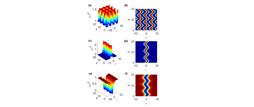
Figure 1: Evolution of (a)-(b) the periodic wave profile (30), (c)-(d) the bright self-similar intensity wave profile (44), and (e)-(f) the dark rational self-similar intensity wave profile (50). The parameters are defined in the text.

First, we concentrate on the most interesting situation when the fiber system does not subject to the influence of the gain effect (i.e., $g_{0}=0$). Figures 1(a) and 1(b) depict the evolution of the self-similar periodic wave (30) for the parameter values: $\alpha_{0}=-1.2,$ $\gamma_{0}=0.756,$ $\sigma=0.8036,$ $p=1,$ $k=0.6,$ $\delta=0.59$ and $\xi_{0}=0.$ The results for the self-similar bright solitary wave (44) are shown in Figs. 1(c) and 1(d) with the same parameter values as that in Fig. 1(a) except $\delta=-0.46$. Figures 1(e) and 1(f) show the evolution of the self-similar dark rational-solitary wave (50) for the parameter values: $\alpha_{0}=1.2,$ $\gamma_{0}=0.6,$ $\sigma=-0.5,$ $p=1,$ $\delta=0.416$. These figures show clearly that the self-similar structures display a snakelike behaviour along the propagation distance due to the presence of periodic distributed dispersion parameter $\alpha(z).$ For such oscillatory trajectory, the self-similar waves keep no change in propagating along optical medium although its position oscillate periodically (which is called “Snakelike” in Ref. ZY ).

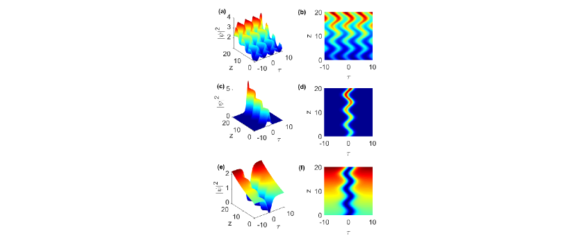
Figure 2: Evolution of (a)-(b) the periodic wave profile (30), (c)-(d) the bright self-similar intensity wave profile (44), and (e)-(f) the dark rational self-similar intensity wave profile (50) when $g_{0}=0.02$. The other parameters are the same as in Fig. 1(a), 1(c) and 1(e), respectively.

We now consider the situation $g_{0}\neq 0$, corresponding to the presence of gain effect in the periodic distributed system described by Eqs. (51) and (52). The evolution dynamics of the periodic wave solution (30), bright solitary wave solution (44) and dark rational-solitary wave solution (50) are presented in Figs. 2(a)-(b), 2(c)-(d) and 2(e)-(f), respectively for $g_{0}=0.02$. One can see that the intensity of propagating waves increase continuously and the time shift and the group velocity of the nonlinear waves are changing while the waves keep their shapes in propagation along the fiber. Hence the gain parameter has no effects on the width or shape of the nonlinear waves and affects only the evolution of their peak.

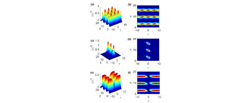
Figure 3: Evolution of (a)-(b) the periodic wave profile (30), (c)-(d) the bright self-similar intensity wave profile (44), and (e)-(f) the dark rational self-similar intensity wave profile (50) when $g(z)=\sin(z)$. The other parameters are the same as in Fig. 1(a), 1(c) and 1(e), respectively.

Second we investigate the self-similar periodic and solitary wave dynamics through a distributed gain amplifier with a periodically varying gain parameter of the form JF : $g(z)=\sin(z).$ The corresponding intensity profiles of periodic, bright and and dark rational-solitary waves are displayed in Figs. 3(a)-(b), 3(c)-(d) and 3(e)-(f), respectively for the same values of parameters as those in Figs.1 (a), 1(b) and 1(c) respectively. For this case, we get periodic emergence of periodic waves in the inhomogeneous fiber system due to the presence of periodic gain, as seen in figure 3(a)-(b). It is obvious that the feature of the bright and dark rational-solitary wave solutions is the same as shown in Fig. 3(c)-(d) and 3(e)-(f), respectively.

We also investigated the dynamical behaviour of the self-similar periodic and solitary waves in a distributed fiber system whose second-order dispersion and gain parameters are distributed according to JF :

$$\alpha(z)=\tanh(z),$$ (55)

$$g(z)=\sin(z).$$ (56)

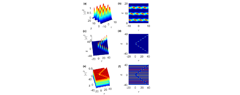
Figure 4: Evolution of (a)-(b) the periodic wave profile (30), (c)-(d) the bright self-similar intensity wave profile (44), and (e)-(f) the dark rational self-similar intensity wave profile (50) when $g(z)=\sin(z)$ and $\alpha(z)=\tanh(z)$. The other parameters are the same as in Fig.1(a), 1(c) and 1(e), respectively.

Figures 4(a)-(b), 4(c)-(d) and 4(e)-(f) present the nonlinear evolution of the self-similar periodic, bright- and dark-solitary-wave solutions (30), (44) and (50) for the same values of parameters as those in Figs.1 (a), 1(b) and 1(c) respectively. We observe that an interesting periodic emergence of periodic, bright and dark rational-solitary waves appear under the influence of this choice of dispersion and gain management.

It is interesting to note that we can also design some other profiles of dispersion and gain parameters to control the dynamical behaviour of propagating self-similar waves. We note that if the dispersion and gain profiles are suitability chosen which may be realistic to some control systems, we can obtain many kinds of self-similar structures with different shapes through modulation of these parameters.

VI Numerical stability analysis

For the sake of completeness, we now analyze the stability of the obtained periodic and solitary wave solutions with respect to finite perturbations. Here we still take the periodic wave (30), bright solitary wave (44) and dark rational-solitary wave (50) as examples to study the structural stability of these self-similar solutions under the perturbation of the additive white noise. Then, we perform a direct numerical simulation of Eq. (1) by employing the split-step Fourier method Agraw , to test the stability of solutions (30), (44) and (50) with initial white noise, as compared to Figs. 1(a), 1(c) and 1(e). As usual, we put the noise onto the initial profile, then the perturbed pulse reads JD : $\psi_{\text{pert}}=\psi(\tau,0)[1+0.1\,$ random$(\tau)].$

Figure 5: The numerical evolution of (a) the periodic wave solution (30), (b) the bright solitary wave solution (44), and (c) the dark rational solitary wave solution (50) under the perturbation of white noise whose maximal value is $0.1$. The parameters are the same as in Figs. 1(a), 1(c) and 1(e) respectively.

Figures 5(a), 5(b) and 5(c) present the evolution of nonlinear wave solutions (30), (44) and (50) under the perturbation of $10\%$ white noise respectively. The numerical results demonstrate that the periodic and solitary waves can propagate stably under the initial perturbation of white noise. Although we have shown here the results of stability study only for three examples of the model (1), similar conclusions hold for other solutions as well. Therefore, we can conclude that the solutions we obtained are stable and should be observable in optical fiber amplifiers.

VII Conclusion

We have studied the self-similar dynamics of picosecond light pulses generating in optical fiber amplifiers and fiber lasers within the framework of the generalized nonlinear Schrödinger equation that takes distributed first and second order dispersions, cubic nonlinearity and gain into account. We have developed a new self-similarity technique which enables us to derive a rich variety of periodic and solitary wave solutions for the model. The self-similar variables and formation conditions for the existence of these self-similar structures are presented. The dynamical behaviour of self-similar periodic and solitary waves has been discussed in a dispersion periodic changing fiber for different gain profiles. The stability of these structures is also investigated numerically by adding white noise. It is proven that these nonlinear self-similar waves can propagate without distortion and should therefore be observable in optical fiber amplifiers which have a Kerr nonlinear response. In view of the increasing relevance of the generalized NLS equation with distributed coefficients in describing the propagation phenomena in several physical media, we anticipate that the results presented here will open new research opportunities and may have practical implications in experiments.

References

- (1) V.N. Serkin, A. Hasegawa, T.L. Belyaeva, J. Modern Opt. 57, 1456–1472 (2010).
- (2) J.F. Zhang, Q. Tian, Y.Y. Wang, C.Q. Dai, and L. Wu, Phys. Rev A 81, 023832 (2010).
- (3) Y. Kodama and A. Hasegawa, Opt. Lett. 7, 339-341 (1982).
- (4) K. D. Moll, A. L. Gaeta, and G. Fibich, Phys. Rev. Lett. 90, 203902 (2003).
- (5) F. Ö. Ilday, J. R. Buckley, W. G. Clark, and F.W. Wise, Phys. Rev. Lett. 92, 213902 (2004).
- (6) A. S. Kewitsch and A. Yariv, Opt. Lett. 21, 24-26 (1996).
- (7) T. M. Monro, P. D. Miller, L. Poladian, and C. M. de Sterke, Opt. Lett. 23, 268–270 (1998).
- (8) S. An and J. E. Sipe, Opt. Lett. 16, 1478–1480 (1991).
- (9) D. Anderson, M. Desaix, M. Karlsson, M. Lisak, and M. L. Quiroga-Teixeiro, J. Opt. Soc. Am. B 10, 1185- 1190 (1993).
- (10) R. Pal, S. Loomba, C.N. Kumar, Annals of Physics 387, 213-221 (2017).
- (11) H. Triki, K. Porsezian, K. Senthilnathan, and K. Nithyanandan, Phys. Rev E 100, 042208 (2019).
- (12) V. I. Kruglov and H. Triki, Phys. Rev A 102, 043509 (2020).
- (13) H. Triki, Q. Zhou, A. Biswas, S.L. Xu, A. K. Alzahrani, M. R. Belic, Opt. Commun. 468, 125800 (2020).
- (14) V. I. Kruglov and H. Triki, Phys. Rev A 103, 013521 (2021)
- (15) H. Triki and V. I. Kruglov, Chaos, Solitons and Fractals 143, 110551 (2021).
- (16) G. I. Barenblatt, Scaling, Self-similarity, and Intermediate Asymptotics (Cambridge University Press, Cambridge, UK, 1996).
- (17) V. I. Kruglov, A. C. Peacock, and J. D. Harvey, Phys. Rev. Lett. 90, 113902 (2003).
- (18) M. Desaix, L. Helczynski, D. Anderson, M. Lisak, Phys. Rev. E 65, 056602 (2002).
- (19) J.D. Moores, Opt. Lett. 21, 555 (1996).
- (20) V. I. Kruglov, A. C. Peacock, and J. D. Harvey, Phys. Rev E 71, 056619 (2005).
- (21) V. I. Kruglov, A. C. Peacock, J. D. Harvey, and J. M. Dudley, J. Opt. Soc. Am. B 19, 461-469 (2002).
- (22) C.Q. Dai, S. Zhu, J. Zhang, Opt. Commun. 283, 3784-3791 (2010).
- (23) C.Q. Dai, Y.Y. Wang, X.G. Wang, J. Phys. A: Math. Theor. 44, 155203 (2011).
- (24) V. N. Serkin and A. Hasegawa, Phys. Rev. Lett. 85, 4502 (2000).
- (25) L. Wang, L. Li, Z. Li, G. Zhou, and D. Mihalache, Phys. Rev. E 72, 036614 (2005).
- (26) S. Konar, M. Mishra, and S. Jana, Fiber Integr. Opt.24, 537 (2005).
- (27) S. Loomba and H. Kaur, Phys. Rev. E 88, 062903 (2013).
- (28) C. Q. Dai, G. Q. Zhou, and J. F. Zhang, Phys. Rev. E 85, 016603 (2012).
- (29) Z.-Y. Yang, L.-C. Zhao, T. Zhang,Y.-H. Li, and R.-H. Yue, Phys. Rev. A. 81, 043826 (2010).
- (30) J. F. Zhang, C. Q. Dai, Q. Yang, J. M. Zhu, Opt. Commun. 252 (2005) 408-421.
- (31) A. Choudhuri, H. Triki, and K. Porsezian, Phys. Rev. A 94, 063814 (2016).
- (32) G. P. Agrawal, Nonlinear Fiber Optics, 4th ed. (Academic, Boston, 2006), Chap. 2.
- (33) J. R. He and H. M. Li, Phys. Rev. E 83, 066607 (2011).