redictably Serving Unpredictable DNNs

Abstract

Existing DNN serving solutions can provide tight latency SLOs while maintaining high throughput via careful scheduling of incoming requests, whose execution times are assumed to be highly predictable and data-independent. However, inference requests to emerging dynamic DNNs – e.g., popular natural language processing (NLP) models and computer vision (CV) models that skip layers – are data-dependent. They exhibit poor performance when served using existing solutions because they experience large variance in request execution times depending on the input – the longest request in a batch inflates the execution times of the smaller ones, causing SLO misses in the absence of careful batching.

In this paper, we present a dynamic DNN serving system, that captures this variance in dynamic DNNs using empirical distributions of expected request execution times, and then efficiently batches and schedules them without knowing a request’s precise execution time. ignificantly outperforms state-of-the-art serving solutions for high variance dynamic DNN workloads by 51–80% in finish rate under tight SLO constraints, and over 100% under more relaxed SLO settings. For well-studied static DNN workloads, eeps comparable performance with the state-of-the-art.

1 Introduction

Deep neural network (DNN) model inference requests constitute an increasingly larger portion of today’s web requests [21, 54]. For example, NVIDIA estimated that 80–90% of the cloud AI workload was inference processing [29]. It is only likely to increase for the foreseeable future with the proliferation of DNN-powered APIs [15, 14] that enable applications to build on top of pre-built foundation models [6].

The underlying serving systems [10, 34, 43, 49, 18] that handle these inference requests aim to maximize throughput while reducing service level objective (SLO) misses. Due to the high throughput and low latency requirements of DNN-dependent applications and the large computation needs of DNN inference requests, modern serving systems often rely on expensive GPUs to serve many requests in parallel by batching them together [18]. All the requests in the same batch experience the same request execution time. This works well because the state-of-the-art DNN serving systems [10, 49, 18] have so far assumed data-independence of incoming requests; i.e., the amount of computation required for each request is the same regardless of the input data. For example, for an image classification model, whether the input image contains a dog or a cat, the model performs exactly the same computation to derive the answer. Consequently, the request execution time of a model can be accurately profiled and used to precisely schedule inference requests [18].

We observe that the recent rise of a new class of dynamic DNNs [52, 19] challenges this assumption (Section 2.2). Unlike static DNNs, dynamic DNNs can adapt their structures or parameters to the input during inference and are thus inherently data-dependent. For example, SkipNet [53] dynamically skips layers depending on the input sample; RDI-Nets [24] allows for each input to adaptively choose one of the multiple output layers to output its prediction; and various NLP models exhibit recurrent structures or loops [58, 30, 33, 51, 41, 42]. The result is unpredictable execution times for individual requests. Because request execution times come from a distribution instead of being a single constant, existing systems that use a single mean or tail execution time from historical data to plan ahead perform poorly [18, 49]. They fail to capture the high variance in incoming requests’ execution times, and when they batch multiple requests together, one long request in the batch slows down many short ones, leading to large number of SLO misses (Section 2.3). Serving systems that do not assume data independence [10, 9, 43] and instead perform reactive adjustment to dynamically provision workers at runtime perform even worse, because they treat SLOs as long-term reactive targets and cannot effectively curtail tail latency, especially under stringent SLO constrains [18].

In this paper, we present distribution-aware dynamic DNN serving system, to provide high throughput and low SLO misses. lso takes a plan-ahead approach, but unlike recent solutions, it uses a random variable to capture the variance in request execution times of dynamic DNNs, rather than assuming a constant mean or tail latency for all requests. This gives ore flexibility to account for uncertainty in execution times when batching them together to achieve high throughput.

Going beyond prior distribution-based solutions for cluster scheduling and query processing [7, 37, 17], ddresses two challenges unique to model serving. First, batching is vital to achieve high throughput, but it also affects execution times, as all requests in the same batch start and finish at the same time, regardless of their individual execution times. roposes a batch-aware priority score that derives batch execution time distributions given those of individual requests, and uses the score to guide its batching decisions. Second, because a model can receive requests from different applications, the joint distribution can be multimodal with even higher variance. To this end, ags each request with its originating application and relies on probability theory to accurately estimate batch execution times even when execution times of requests in the same batch follow different distributions.

We have implemented and evaluated sing production traces and a large range of possible input execution time distributions (Section 5). In comparison to Clockwork [18], Nexus [49], and Clipper [10], an improve the finish rate when serving dynamic DNNs by 51–80% under tight SLO constraints, and over 100% under more relaxed SLO settings. For well-studied static DNN workloads, eeps comparable performance with the state-of-the-art.

Overall, we make the following contributions in this paper:

• To the best of our knowledge, s the first system to systematically analyze the inference performance of dynamic DNNs and associated challenges.

• We present a batch-aware distribution-based scheduling algorithm to handle batching and multimodal distributions in dynamic DNN serving systems.

• an handle both static and dynamic workloads with high throughput and tight SLO guarantees.

2 Background and Motivation

In this section, we overview model serving systems and the recent rise of dynamic DNNs, and then move on to the limitations of existing state-of-the-art solutions when serving such dynamic networks.

2.1 Model Serving

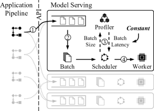
Figure 1: A model serving service multiplexes requests from multiple applications and schedules batches of requests on workers.

Increasingly more models are deployed on the critical paths of online interactive services [54]. They may even comprise dependent computations across multiple models, forming pipelines [9]. For example, video analytics pipelines first detect certain objects from each image and then recognize individual objects [56, 49]. A serving system in the backend handles inference requests for individual models by running a model replica on the input, usually providing APIs for specific tasks such as detection, translation, or prediction [15, 14]. Similar to other datacenter services [1], it multiplexes workloads of different applications and load balances requests across multiple workers [43, 10].

Lifecycle of Serving Inference Requests

Figure 1 illustrates the lifecycle of (a batch of) inference requests in a worker of such serving systems. Incoming requests first go through a priority queue, usually ordered by deadline, but it may vary depending on a system’s optimization goal. The dynamic batcher will extract requests from the queue to create batches, while respecting the deadline requirement of the requests at the top of the queue. The size of the formed batch will be queried against historical profiling data to decide an estimated batch latency. This single latency value will be used in the scheduler to derive an execution plan on the worker. Of course, there is not exactly one way to divide work between the stages shown here, and there may be additional interactions between various components. For example, Nexus [49] uses a pre-computed plan ahead of time, while Clockwork [18] employs multiple “Batch Queues” to select the best batch size at runtime. Nevertheless, the active state in these systems depends on a single, point estimation of the batch latency, oblivious to individual request-specific data at runtime.

Batching and the Throughput-Latency Tradeoff

To achieve high throughput, model serving systems [18, 49, 10, 9, 43] rely on batching multiple requests. Requests arriving within a specific time window are batched together to ensure that worker resources do not idle [10, 49]. There is, however, a tradeoff in picking a batch size. While a larger batch size may increase throughput, it also means longer time window; the latter can lead to higher (tail) latency and missed SLOs. In contrast, a smaller batch size can result in underutilized hardware. Existing solutions focus on finding the sweet spot to reduce SLO misses, typically for each model individually [18, 49, 10, 43], while pipeline-aware solutions break down the end-to-end SLO into smaller pieces [9]. The overall objective of a model serving system can, therefore, be described as maximize throughput while reducing SLO misses.

2.2 Dynamic DNNs

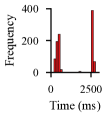
(a) RDI-Nets

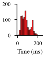
(b) GPT

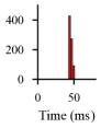
(c) Inception V3

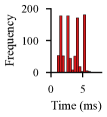
(d) SkipNet

(e) BART

(f) ResNet

Figure 2: Inference request execution time varies widely in dynamic CV and NLP models. (Inception V3 and ResNet are shown for comparison.)

Point estimations in existing solutions is sufficient only because they focus on static DNNs (e.g., CNNs), where each request roughly takes the same amount of time and is highly predictable [18]. However, we observe that dynamic DNNs are becoming increasingly more popular in recent years [6, 19]. Dynamic DNNs adapt their structures or parameters to different inputs, leading to notable advantages in terms of accuracy, computational efficiency, adaptiveness, etc., compared to static DNNs that have fixed computational graphs and parameters at the inference stage [19]. Examples of dynamic DNNs include various language models [12, 52] as well as early-exit techniques used in emerging CNN models [53].

Observation: Dynamic DNN Inference is Unpredictable

As the name suggests, the computation requirement of inference requests to a dynamic DNN model can be dynamic. It naturally follows that the request execution time is no longer constant for different inputs anymore. We report inference execution time histograms for four common dynamic networks (SkipNet [53], RDI-Nets [24] for image recognition, GPT [58], BART [30] for NLP) in Figure 2. For comparison, we also include the execution time for two common static CV models: Inception V3 [50] and ResNet [22]. Note that the absolute number of requests in these histograms is less important, as it merely represents the testing dataset we used. However, the existence of a large range of values in the x-axis reflects the possibility of different execution times.

For the image recognition models, there are a few distinct clustered ranges, which represent multiple code paths with different execution times, created by skipping/choosing parts of the model. Similar observations hold for NLP models too. However, instead of having distinct code paths, execution time for NLP models falls in a continuous range, reflecting the impact of the input sequence length on execution time. Nevertheless, it can be seen that the difference in inference latency can be as large as $10\times$, with some requests finishing in $10$ms while many others taking more than $100$ms.

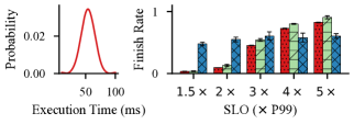
(a) Simple normal distribution

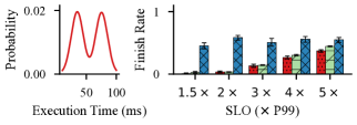
(b) Bimodal distribution

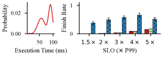
(c) Bimodal distribution w/ inequal peaks

Figure 3: Performance of existing model serving solutions for dynamic DNNs. Similar results hold for more diverse distributions as well (Section 5).

Challenges in Serving Dynamic DNNs

The presence of a large variance in execution times of dynamic DNNs as well as the shared nature of model-serving-as-a-service systems lead to two key challenges when serving dynamic DNNs.

1. Effective batching: Batching is a must for high throughput and worker utilization. However, all requests in the same batch start and finish at the same time, regardless of their individual execution times. When requests in the same batch vary widely in their execution times, the longest one becomes the straggler and slows down the entire batch.

2. Handling multimodal distribution: A model built for a specific task (e.g., classification, translation, etc.), is often used by multiple applications, especially when it is exposed as a service. As a result, input requests and their corresponding execution times often follow different application-specific distributions. The combined multimodal distribution has even higher variance, which can introduce even more stragglers during batching.

2.3 Limitations of Existing Solutions

Indeed, state-of-the-art model serving solutions [49, 10, 18], which have been optimized for static DNNs, suffer from high SLO violation rates when applied to dynamic DNNs. Figure 3 shows the finish rates of three recent model serving systems when the input execution time follows various distributions, under different SLO settings. For each case, the probability distribution function (PDF) of the input execution times is shown to the left. For all cases, the incoming rate trace is derived from the Microsoft Azure Functions workload trace [48] similar to Clockwork [18]. Section 5 provides more details on the methodology.

The high-level takeaway is that all these systems have undesirable performance. As most batches contain both long requests and short ones, the execution time for the whole batch is almost always longer than the average. This causes Clockwork [18] to often mispredict a batch’s latency, which in turn leads to frequent time-out error in its scheduler, causing the subsequent batch to fail. This explains its close-to-half finish rate. Nexus [49] pre-computes an execution plan ahead of time using the average execution time, but due to the variance in input execution, it cannot reach a stable state. Clipper [10] monitors request execution time reactively, but it cannot keep up under tight SLO settings. Fundamentally, we observe the effect of existing solutions failing to batch requests effectively.

Distribution-Based Schedulers

Existing distribution-based schedulers such as 3Sigma [37] or Shepherd score [7], proposed for cluster scheduling and query processing respectively, do not fare well either. They do not consider sub-second level latency constraints or inference serving-specific challenges like batching and lack of preemption.

3 verview

s an inference serving system that serves inference requests to a dynamic DNN model while maximizing the number of requests that can be served within the SLO. In this section, we provide an overview of how its in the inference life cycle of dynamic DNNs to help the reader follow the subsequent sections.

3.1 Problem Statement

Each inference request in s defined by its release time and deadline (release time plus SLO), and has a minimum execution time that is measured when the request is executed alone. Multiple applications with diverse use cases and corresponding input distributions send requests to the same dynamic DNN model served by Each GPU worker processes these requests one batch at a time. Note that, to scale out to a pool of workers in a cluster setting, different models and their replicas can use n parallel.

Given a set of pending inference requests, the cheduler must decide which subset of them should be included in the next batch submitted to the GPU to maximize throughput while reducing SLO misses, under the following constraints:

• Partial information: the execution time of a request, and thus a batch, is unknown to the scheduler. However, its probabilistic distribution can be learned from historical data.

• Non-preemption: inference execution of a batch cannot be preempted after it is submitted to the GPU.

3.2 rchitecture

Unlike existing model serving systems, epresents the request execution time of a dynamic DNN model as a random variable, which is described using an empirical distribution over a time window. Thereafter, instead of using simply the mean or the max of the population, it makes scheduling decisions using the knowledge of the entire distribution.

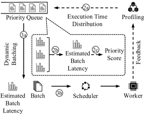
Figure 4: rchitecture.

ddresses the challenges arising from multimodal distribution and effective batching by proposing a time-varying priority score (detailed in Section 4) by considering a batch’s combined distribution. It determines this priority score for all requests that potentially can be put together to form a batch, and then it performs priority-based scheduling.

Inference Lifecycle

As shown in Section 3.2, ollows the same overall process as other model serving systems, but with updated scheduling steps and in Figure 1:

1. incoming requests are tagged per application, and the application-specific execution time distribution is associated with each request using the information collected by s online profiler;

2. execution time distributions from requests are combined to derive estimated batch execution time (latency);

3. next, the priority score for all requests are calculated using the estimated request latency, deadlines and the current time as input;

4. alculates estimated batch latency for all potential batch sizes;

5. the scheduler loop selects a feasible batch size to actually create the batch.

   After obtaining a batch, ubmits it to the worker for execution, following the same step as existing model serving systems.

   Next, we elaborate on s scheduling loop and its batch handling.

   Batch Size Selection

   It is not always possible to execute requests using the maximum possible batch size, because some requests may have tighter deadlines than others and waiting for the maximum batch size can take too long.

   racks the set of feasible batch sizes for each request. These sets of feasible batch sizes are updated over time. When the deadline is approaching, batch sizes that are too large to meet the deadline will be dropped, so the corresponding request will only be considered for small batches. In addition, for each batch size, eeps note of the earliest deadline for requests suitable for the batch size. The batch size with the overall earliest deadline will be chosen by the scheduler to lazily create a batch and send to the worker for execution.

   Algorithm 1 shows s scheduling loop, which implements the above batch size selection scheme (Algorithm 1 to Algorithm 1). It is worth noting that ses a separate priority queue $Q_{\mathit{bs}}$ for each batch size $\mathit{bs}$. The earliest deadline for requests in $Q_{\mathit{bs}}$ is tracked by an additional Fibonacci heap to allow online deletion.

   Batch Priority

   The highest priority batch is the one to be scheduled next, and it depends on the priorities of individual requests. ses a time-varying score for request priority, i.e., the priority of a request changes over time. Naively sorting the pending requests’ queue in $O(n\log n)$ time for each scheduling iteration in the hot path is inefficient. Instead, we use an $O(\log^{2}n)$ priority queue [8, 7]. We also address issues related to floating-point overflow when using such queue in practice (Section 4.4).

   1

   2

   3

   Input:

   $\mathcal{R}\leftarrow$ set of pending requests,

   $t\leftarrow$ current time,

   $\mathcal{S}\leftarrow$ set of batch sizes suported by the model,

   $Q_{\mathit{bs}}\leftarrow$ set of requests viable for batch size $\mathit{bs}$,

   $D_{r}\leftarrow$ deadline of request $r$,

   $D_{Q_{\mathit{bs}}}\leftarrow$ $\min\{D_{r}|r\in Q_{\mathit{bs}}\}$,

   Output: Batch $\mathcal{B}\subseteq\mathcal{R}$

   4

   $\triangleright$ Update priority scores (Section 4.4)

   5

   $U\leftarrow\emptyset$

     $\triangleright$ requests needs to be updated

   6

   7if need reset base time then

   8       reset base time

   9       $U\leftarrow\mathcal{R}$

   10      

   11for $r\in\mathcal{R}$ do

   12       if $t\geq\textnormal{{Milestone(}}\textnormal{\emph{r}}\textnormal{{)}}$ then

   13             $U\leftarrow U\cup\{r\}$

   14      

   15for $r\in U$, $\mathit{bs}\in\mathcal{S}$ do

   16       update priority score of $r$ in $Q_{\mathrm{bs}}$

   17

   $\triangleright$ Drop requests from queue if too late

   18

   19for  $\mathit{bs}\in\mathcal{S}$, $r\in Q_{\mathit{bs}}$ ordered by $D_{r}$  do

   20       if $t+\textnormal{{EstimateBatchLatency(}}\textnormal{\emph{r, bs}}\textnormal{{)}}>D_{r}$ then

   21             $Q_{\mathit{bs}}\leftarrow Q_{\mathit{bs}}\setminus\{r\}$

   22            

   23      

   24      if $\mathit{bs}$ is the last feasible batch size for $r$ then

   25             Mark $r$ as timed out

   26            

   27      

   28

   $\triangleright$ Determine candidate batch size

   29 $\mathit{candidate}\leftarrow\mathsf{nil}$

   30 for $\mathit{bs}$ ordered by ($D_{Q_{\mathit{bs}}}$, $\mathit{bs}$) in descending order do

   31       if $\lvert Q_{\mathit{bs}}\rvert\geq\mathit{bs}$ then

   32             $\mathit{candidate}\leftarrow\mathit{bs}$

   33             break

   34            

   35      

   36if $\mathit{candidate}$ is $\mathsf{nil}$ then

   37       return

   38      

   $\triangleright$ Select top ones ordered by core

   39 return $\mathcal{B}\leftarrow$ PopBatch($Q_{\mathit{candidate}}$)

   Algorithm 1 cheduler Iteration

   Before proceeding to the details of s algorithm in the next section, we highlight a few other components in

   Per-Application Tracking

   As shown in , ssociates each request an execution time distribution using application-specific historical data. First, it is possible to distinguish requests from application as there are usually certain application IDs involved when the model is exposed as a service. Second, such tracking is also necessary, because applications may solve problems in different domains despite using the model for the same task. As a result, input requests execution times often follow different distributions. While oes not assume any pre-defined distribution for its input and only tracks empirical distributions, the combined multimodal distribution has higher variance. This hurts scheduling abilities even if the scheduler has perfect information of its distribution, because the scheduler has to account for different possibilities when scheduling.

   Long-Term Feedback Loop

   Incoming requests can change their arrival pattern and volume over time, either due to the diurnal nature of the service or due to shifts in general interests. herefore needs to track per application execution time data for requests over time. However, our calculation needs the execution time for requests when they execute alone, which cannot be guaranteed if simply measuring the time online. Instead, the profiler in akes an asynchronous approach. Finished requests are sampled and send to the profiler to evaluate individually. The execution time data will then be asynchronously picked up and accumulated by the scheduler periodically, completely off the critical path. In order to adapt to drifts in the input, esets its profiling memory every once a while. The exact window is configurable and is determined by domain knowledge.

   4 Batch-Aware Distribution-Based Scheduling

   At its core, s a priority-based scheduler where the priorities of individual requests are determined using a cost function that captures the distribution of request execution times. Highest priority requests are then put in a batch to achieve the maximum level of parallelism, which is then submitted to the worker. To achieve this, elies on probability theory to accurately estimate request execution times even when requests in the same batch affect each other and their executions are no longer independent.

   In this section, after a brief introduction of cost function and the definition of priority on a single request (Section 4.1), we dive into the derivation of a vital term in the batch-aware priority score – batch execution time, given request execution time following the same distribution (Section 4.2.1) and different distributions (Section 4.2.2). Finally, we discuss how to break the cyclic dependency between batch formation and priority score computation (Section 4.3), as well as floating-point overflow handling when applying the algorithm in practice (Section 4.4).

   4.1 Preliminaries

   Cost Function

   Instead of directly optimizing for metrics such as average/tail latency and throughput, we model SLO deadlines using a cost function that captures the opportunity cost differences between two important scheduling decisions. On the one hand, executing a request involves costs for resource usage (e.g., server utilization) and opportunity cost (e.g., it may postpone other requests). On the other hand, missing deadline may have a monetary penalty according to the SLO. Throughout the rest of the paper, we use SLO cost functions similar to that in Figure 5. Meaning, for requests arriving at time $T$ with deadline $D$, there is a penalty $c$ for missing that deadline.

   Scheduler Objective

   The objective of our scheduler is to minimize the overall cost, or as we set out to do, maximize the number of requests that finish within corresponding deadlines. Selecting a request to put into the next batch reduces the expected cost that would have been incurred if it were delayed. Therefore, our goal is to find requests for which the ratio of expected cost reductions are the greatest.

   Background: Priority of a Single Request

   Consider a request whose execution time $L$ is a random variable and its cost function is $C(t)$. Cost reduction for this request boils down to the difference between the costs of two scheduler decisions: $C_{\mathit{now}}(t)$, including the request in the next batch and executing it right away, or $C_{\mathit{delay}}(t)$, selecting another one and thus delaying this request.

   Its priority $p(t)$ can thus be defined as:

   $$p(t)=\frac{1}{\operatorname*{\mathbb{E}}[L]}\left(\operatorname*{\mathbb{E}}[C_{\mathit{delay}}(t)]-\operatorname*{\mathbb{E}}[C_{\mathit{now}}(t)]\right)$$ ((1))

   Note that $C_{\mathit{now}}(t)=C(t+L)$ is a random variable, as well as $C_{\mathit{delay}}(t)=C(t+\tau+L)$ ($\tau$ is the anticipated delay).

   Given that $C(t)$ has the same shape as in Figure 5, and assuming $\tau$ follow an exponential distribution with parameter $b$, prior work [7] has shown that, when $L$ can be described using a histogram, $p(t)$ can be derived by computing on each histogram bin separately and combining the results:

   $$p(t) =\sum_{i}p_{i}(t)$$ ((2))

   $$p_{i}(t) =\begin{cases}\frac{hc}{\operatorname*{\mathbb{E}}[L]b}\left(e^{bl^{(i)}_{2}}-e^{bl^{(i)}_{1}}\right)e^{-bD}e^{bt}&t<D-l^{(i)}_{2}\\ \frac{hc}{\operatorname*{\mathbb{E}}[L]b}-\frac{hc}{\operatorname*{\mathbb{E}}[L]b}e^{bl_{1}}e^{-bD}e^{bt}&D-l^{(i)}_{2}\leq t<D-l^{(i)}_{1}\\ 0&D-l^{(i)}_{1}\leq t\end{cases}$$

   where $p_{i}(t)$ is the score for the $i$-th bin in the histogram with range $[l^{(i)}_{1},l^{(i)}_{2})$ and frequency $h$. We represent the deadline for the request in consideration using $D$, with $c$ being the cost when missing the deadline.

   

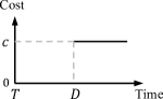
   Figure 5: An example of SLO cost function.

   4.2 Batch Latency Estimation

   We still need to find out the distribution of $L$, as well as $\operatorname*{\mathbb{E}}[L]$. As we discussed in Section 2.1, the scheduler must schedule batches of requests to ensure high throughput. This is an important detail, because up until now, we assumed the execution time $L$ as an intrinsic property of the request, depending solely on the request itself. However, under the batch execution model, it is no longer the case: requests do not execute alone, and they affect each other’s execution time in the same batch. The purpose of the term $\frac{1}{\operatorname*{\mathbb{E}}[L]}$ in Eq. (1) is to account for the worker time usage of the request. As such, to accurately represent a request’s potential worker time usage during batching, $L$ must now be the execution time of the whole batch the request is in.

   When the request execution time itself is a constant (i.e., in static DNN scenarios), this is trivial: requests are homogeneous; so is the batch. It is thus possible to profile the batch execution time for all possible batch sizes ahead of time [18]. In our case, however, not only are requests’ execution times random variables, but a batch may also contain requests from different duration distributions. Next, we describe how andles batches of requests following the same or different distribution separately.

   4.2.1 Requests in Batch Follow the Same Distribution

   For a batch $B$ of $k$ requests, if requests are of the same duration $l$, the batch execution time $l_{B}$ could be fairly assumed (within reasonable range) as

   $$l_{B}=c_{0}+c_{1}kl$$ ((3))

   where $c_{0}$ and $c_{1}$ are constant parameters specific to a model and hardware.

   In the case of dynamic models, requests in a batch are padded to the largest one and therefore, it can be viewed as if the whole batch’s requests have the same length:

   $$l=\max_{r\in B}l_{r}$$ ((4))

   Then the execution time of $B$ becomes a new random variable $L_{B}$. With $L_{r}$ as the random variable of request $r$’s execution time, we have

   $$\operatorname*{\mathbb{E}}[L_{B}] =c_{0}+c_{1}k\operatorname*{\mathbb{E}}[\max_{r\in B}l_{r}]$$ ((5))

   $$=c_{0}+c_{1}k\int_{0}^{\infty}L_{r(k)}f_{L_{r(k)}}(l)\mathop{}\!\mathrm{d}l$$

   where $L_{r(k)}$ is $L_{r}$’s max order statistics over $k$ samples, and $f_{L_{r(k)}}(l)$ is its PDF. While it is possible to directly find out $f_{L_{r(k)}}(l)$, it is easier to go through the cumulative distribution function (CDF) of $L_{r(k)}$ first, denoted as $F_{L_{r(k)}}(l)$, which is related to the CDF of $L_{r}$ via a simple equation:

   $$F_{L_{r(k)}}(l)=[F_{L_{r}}(l)]^{k}$$ ((6))

   And we can obtain $F_{L_{r}}(l)$ from $L_{r}$’s histogram. Note that while it is possible to directly use $F_{L_{r(k)}}(l)$ to calculate $\operatorname*{\mathbb{E}}[\max_{r\in B}l_{r}]$, the result would be far too inaccurate, as we only have a discrete histogram to start with.

   4.2.2 Requests in Batch Follow Different Distributions

   Taking one step further, if requests $r_{i}(i=1,2,\dots,k)$ in $B$ come from different distributions, the problem becomes finding the max order statistics $L_{r(k)}$ for $k$ random variables $L_{r_{i}}$ that are independent, but not necessarily identically distributed.

   Let $F_{i}$ and $f_{i}$ be the CDF and PDF for $L_{r_{i}}$, respectively, and define $F^{s},f^{s}$ as

   $$F^{s} =\frac{1}{n_{s}}\sum_{i\in s}F_{i}$$ ((7))

   $$f^{s} =\frac{1}{n_{s}}\sum_{i\in s}f_{i}$$

   where $s$ is a subset of requests ($s\subseteq B$) with $n_{s}\geq 1$ elements. The PDF of the maximum (i.e. $k$-th order statistics) of these $k$ variables $f_{(k)}$ is given by Özbey et al. [36]:

   $$f_{L_{r(k)}}=\sum^{k}_{\kappa=1}(-1)^{k-\kappa}\frac{\kappa^{k}}{k!}\sum_{n_{s}=\kappa}k[F^{s}]^{k-1}f^{s}$$ ((8))

   Here $\sum_{n_{s}=\kappa}$ means summation over all possible $s\subseteq B$ where $n_{s}=\kappa$.

   With $f_{L_{r(k)}}$, we can describe the PDF of $L_{B}$ using Eq. (3)

   $$f_{L_{B}}(l)=f_{L_{r(k)}}(\frac{l-c_{0}}{c_{1}k})$$ ((9))

   Similarly, by plugging Eq. (8) into Eq. (5), we can also find out $\operatorname*{\mathbb{E}}[L_{B}]$. We now have complete ingredients to compute the priority score $p(t)$.

   

   (a) Execution time of two types of requests.

   

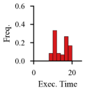
   (b) Execution time histogram for the batch.

   

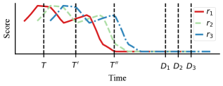
   (c) The priority score of $r_{1},r_{2},r_{3}$ entering the system one after another.

   Figure 6: Toy example of batch execution time estimation and priority score computation.

   A Toy Example

   Let us use an example to illustrate how $p(t)$ changes over time $t$, to put the above discussed equations into perspective.

   Consider two types of requests in total, whose execution time follow two different distributions, as shown in 5(a). While they all have the same mean execution time $l$, the first distribution has higher probability of finishing exactly at $l$, and the second one may either finish very early, or very late. Further, assuming that the batch size in consideration is 2 and there is no overhead for batching (i.e. $c_{0}=0,c_{1}k=1$).

   5(b) shows the histogram of $L_{B}$ that is derived using Eq. (9). As expected, the execution time for the whole batch is skewed to the right, because it is not possible for the shorter execution time in the first distribution to ever become the whole batch’s execution time.

   5(c) illustrates the priority score changing over time for three requests $r_{1},r_{2},r_{3}$ entering the system one after another. At time $T$, $r_{1}$ and $r_{2}$ are the most urgent and should be executed. As the deadline is approaching, $r_{1}$ and $r_{3}$ become the top ones at time $T^{\prime}$. Finally, $r_{2}$ and $r_{3}$ would have been selected as the score for $r_{1}$ drops to 0.

   4.3 Batch Formation

   The last step is forming the batch, which must address a key challenge: the circular dependency between priority calculation and batch formation. $\operatorname*{\mathbb{E}}[L]$ is used in the priority calculation, so the list of possible distributions must be known. However, the batch is determined after priority is computed, and thus it is impossible to know what other requests are in the batch. Assuming that the queue most likely contain requests from all types of applications the model is serving, we therefore always use all execution time distributions associated with the model to compute $\operatorname*{\mathbb{E}}[L]$. As this list of distributions is available ahead of time, and only depends on the batch size, this approach has the additional benefit that the relatively heavy computation can be moved away from the critical path.

   4.4 Efficient Computation

   As shown before, the priority score for a request varies depending on the remaining time before its deadline. It thus has to be re-computed continuously. Combined with the effort to re-sort all pending requests, the naive implementation is not scalable to large number of requests.

   It is possible to convert the problem to dynamic convex hull querying, which can achieve $O(\log^{2}n)$ complexity for each reschedule, where $n$ is the number of pending requests [8]. The dynamic convex hull problem is defined by rewrite each request’s priority Eq. (2) in the form of $p_{i}(t)=\alpha e^{bt}+\beta$, and consider each request to be on a 2D plane with the coordinate $(\alpha,\beta)$. Then, the first point on the convex hull hit by affine lines of slope $-e^{bt}$ corresponds to the request with the highest score at time $t$.

   This way, the problem is divided into one time-invariant part where the relative positions of requests only change a few times (when the relationship between $t,D,l^{(i)}_{1},l^{(i)}_{2}$ changes, corresponding to the Milestone function in Algorithm 1), and one time-varying part – querying the convex hull with a line. Therefore, the priority queue can be implemented by maintaining a convex hull containing all pending requests.

   However, while querying a static convex hull is trivial, our convex hull changes over time as requests come and go. In we use the convex hull algorithm proposed by Overmars and von Leeuwen [35], which supports dynamically adding/removing points on the convex hull in $O(\log^{2}n)$ complexity and can be queried with a line in $O(1)$ time.

   Overflow Handling of Exponential Values

   While the theory works out, there is still a non-trivial challenge that we faced when implementing the priority score in practice.

   In the original Eq. (2), the score only depends on $D-t$ which is the remaining time before the deadline, and is bounded assuming requests too far in the future should not enter the system. However, the clever 2D plane mapping breaks the component into $e^{-bD}$ and $e^{bt}$ individually. Because $D$ and $t$ can be large timestamps (usually represented as elapsed seconds/milliseconds since UNIX epoch), this leads to floating-point overflow when the system tries to compute and store these very large exponential values.

   We compensate this by using relative timestamps for $D$ and $t$, and then choose $b$ wisely. If the time resolution is in milliseconds, and $b=10^{-4}$, we can sustain about $1000~{}\text{s}$ of scheduling before overflows of 64-bit floating-point numbers and having to reset the relative timestamps’ reference point and thus re-calculate everything. Note that the exact value of $b$ does not matter because it does not change the relative ordering of requests as long as it is kept constant.

   5 Evaluation

   Table 1: List of workloads.

   Task	Model	Dataset	Mean Exec. (ms)	P99 Exec. (ms)
   Image classification	RDI-Nets [24]	CIFAR [28]	683.15	2667.54
   Image classification	SkipNet [53]	ImageNet [44]	3.24	5.56
   Chatbot	Blenderbot [42]	convAI [13]	200.39	242.27
   Chatbot	Blenderbot	Cornell [11]	203.22	247.04
   Chatbot	GPT [58]	convAI	79.47	143.40
   Chatbot	GPT	Cornell	94.84	161.69
   Summarization	BART [30]	CNN [47]	774.66	1101.99
   Summarization	T5 [41]	CNN	552.91	797.28
   Translation	FSMT [33]	WMT [5]	189.30	319.31
   Translation	mBART [51]	WMT	432.38	729.87

   

   

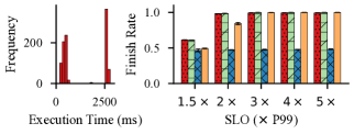
   (a) Image classification/RDI-Nets/CIFAR

   

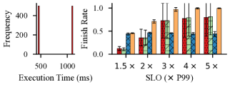
   (b) Summarization/BART/CNN

   

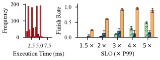
   (c) Image classification/SkipNet/ImageNet

   

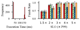
   (d) Chatbot/GPT/Cornell

   Figure 7: erformance on real world tasks. Error bars represent standard deviation across 5 runs.

   We evaluate gainst three existing serving systems (Clipper [10], Nexus [49], and Clockwork [18]). Our primary findings are as follows:

   • Compared to the state-of-the-art, an improve the finish rate when serving dynamic DNNs by 51–80% under extremely tight SLO constrains, or over 100% under more relaxed SLO settings (Section 5.3). At the same time, eeps comparable performance when serving traditional static models (Section 5.4).

   • an sustain thousands of pending requests in its priority queue with less than $0.5~{}\text{ms}$ per-request insertion time (Section 5.5).

   • Our choice of $b$, the anticipated delay distribution parameter (Section 4.1) in the priority score is safe, as s not sensitive to the value of $b$ (Section 5.6).

   • as minimal overheads and can manage requests with execution time varying in ranges as low as $2~{}\text{ms}$–$20~{}\text{ms}$ (Section 5.7).

   5.1 mplementation

   We implemented n top of Clockwork [18], a state-of-the-art serving system with fewer than 4000 lines of C++ code. One-fourth of the new code is for implementing the dynamic convex hull data structure, as there is no established library available for solving the dynamic convex hull problem. Specifically, we implemented the inner concatenate queue as a 2–3 tree extending from the left-leaning-red-black-tree [2, 46].

   5.2 Experimental Methodology

   Testbed

   We built our testbed on Chameleon Cloud [27]. The host has 2 Intel Xeon Gold 6230 CPUs with NVIDIA V100 GPU. In order to have stable results, we fix the GPU clock speed to its maximum $1380~{}\text{MHz}$ and memory clock speed to $877~{}\text{MHz}$.

   We use Ubuntu 20.04 as the base OS environment with the latest NVIDIA GPU driver. We use CUDA versions matching the published original source code, which means CUDA 11.1.1 with CuDNN 8 for Clockwork and CUDA 10.0 with CuDNN 7 for Nexus. For Clipper, its latest commit 9f25e3f is used.

   During experiments, each evaluated system’s server is deployed on the host. Clockwork and dditionally have their serving threads set to high-priority and pinned to physical cores as per Clockwork’s host setup instructions. In addition, the model is modified to allow us to explicitly control its execution time via input for the purpose of evaluation.

   An open loop (no wait for requests completion before issuing the next one) client is used to drive all experiments on the same host to minimize the impact of networking.

   Input Trace

   Similar to workload traces for static models, the request incoming rate trace determines how fast requests coming in and needs to match the system’s load. Same as Clockwork’s evaluation, we adapt the Azure trace [48], which is published by Microsoft for lambda functions. The trace was scaled down such that the incoming rate matches the system load. The incoming rate trace is kept the same across all experiments.

   Request Execution Time Distribution

   Unlike a single number for one model/dataset combination in evaluations in static serving systems, we need a full distribution. We group the model’s associated dataset into short-running and relatively long-running requests (or more groups in case of higher modality), then randomly choose from them to get a mixture of both. To get a fair comparison, the generation is done once among different runs, we then record the arrival time and the input, which will be replayed for subsequent runs.

   Real World Dataset

   We evaluate n a set of real world learning tasks covering both CV ones like image classification, and NLP ones including chatbot, summarization and translation (Table 1). For each workload, the input execution time distribution is determined according to the above-mentioned method, and the P99 of real execution time used to determine SLO is reported in the table.

   Metrics

   We focus on the finish rate, which is defined as the ratio of the number of requests finished in time to the total number of requests. We assume that the SLO is set to a reasonable value manually given historical data, similar to serving static models. Using the P99 tail of all input requests’ real execution time as a measurement, we vary the SLO to be multiples of P99 for most our experiments.

   5.3 Improvements for Dynamic Workloads

   Real World Dataset

   We report representative cases in Figure 7, while the complete results can be found in Appendix A. In most workloads, existing systems can barely make it due to the mixture of long and short requests which rarely match the mean execution time those systems use for scheduling. For RDI-Nets/CIFAR, BART/CNN and GPT/Cornell, an reach near 100% finish rate with sufficient SLO settings. When requests become extremely short (e.g., 6(c)), none of the system can finish many requests due to the too tight latency requirement. However, till manages to finish more requests than others.

   Different Distributions

   We then evaluate s performance under more diverse distributions using the same BART model and with a synthesized dataset to control execution times.

   In Section 5.3, we increase the number of modalities of the distribution to simulate the effect of multiple applications. With the number of modalities increases, the variation in execution time increases. eeps relatively good finish rate and see performance gain as high as $2\times$. The result is consistent with even higher modalities, and we report additional results for up to 8 modals in Appendix A.

   Finish rate under different modality distributions. []

   

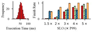
   (a) Simple normal distribution

   

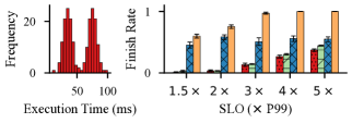
   (b) Bimodal distribution

   

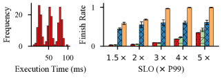
   (c) Three-modal distribution

   

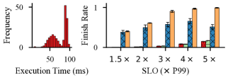
   (d) Bimodal distribution with inequal peaks (more short requests)

   

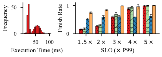
   (e) Bimodal distribution with inequal peaks (more long requests)

   s performance under inequal-peak distributions. []

   The distributions in 7(c) are the same except for mirrored inequal peak locations. However, Clipper and Nexus suffer more in 7(d) because exceptional longer than expected requests are definitely timed out while exceptional shorter than expected requests can still meet the deadline.

   Figure 8 extends on 7(b), whose input request execution time distribution is generated with $\sigma=1$, and explores the effect of smaller ($\sigma=0.5$) and larger ($\sigma=1$) values. Larger $\sigma$ means the peaks are less distinguishable and the degrees of longer requests blocking shorter ones is less severe. s performance remains stable while others see slightly higher finish rate when the separation between requests become less extreme and vice versa.

   Clockwork’s performance is not affected by changes in distributions. As long as the execution time is not constant, it suffers from the same fail-every-other-batch pattern as we discussed in Section 2.3.

   

   

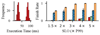
   (f) Bimodal distribution with $\sigma=0.5$

   

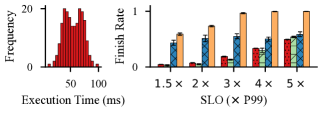
   (g) Bimodal distribution with $\sigma=2$

   Figure 8: Finish rate under different distribution parameters.

   5.4 Improvements for Traditional Workloads

   We next verify s performance under traditional workloads using static models where there is no variance in request execution time.

   Using the ImageNet [44] dataset, we measure the finish rate for four systems when serving the ResNet [22] model and Inception V3 [50] model (Figure 9). ees significant improvement over Nexus and Clipper under tight SLOs ($1.5\times$ and $2\times$), thanks to its plan-ahead scheduling. When compared to Clockwork, upon which s built, due to differences in request handling mechanisms, erforms slightly better when SLO is higher while Clockwork has higher finish rate under tight SLOs, albeit with higher variances.

   

   

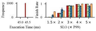
   (a) Inception model on ImageNet

   

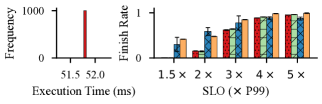
   (b) ResNet model on ImageNet

   Figure 9: eeps comparable performance under workloads where there is no variance in request execution time.

   5.5 Efficiency of the Priority Queue

   To study the efficiency of our priority queue implementation, we evaluate two of the most common operation of the priority queue in isolation: insertion and query. To measure the time it takes to insert a request into the queue, we run micro-benchmarks that fill the queue to certain number of requests, and compute the average insertion time per-request. For query, we first fill the queue and measure the time it takes to query the queue against a line of random slope – the equivalent of finding the request with the highest priority, as discussed in Section 4.4. We vary the number of requests in queue from 10 to 10000, and each data point is averaged over 100 samples. As reported in Figure 10, the insertion operation takes longer as the queue becomes larger, and the overall complexity trend fits the theory $O(\log^{2}n)$ line pretty well. Query time sees large variation when the number of requests is small, but stabilizes and remains constant as the queue size increases. Overall, we can see that thanks to the efficient implementation, thousands of requests can be handled in negligible time, and thus s able to schedule large number of pending requests.

   

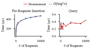
   Figure 10: The insertion time of riority queue under different numbers of requests in queue.

   5.6 Sensitivity to the Anticipated Delay Distribution

   In the priority score calculation in Section 4.1, we introduce a parameter $b$ when describing the distribution of the anticipated delay. And we discussed that in order to avoid floating-point overflow during calculation, we choose $b=10^{-4}$ in Eq. (2). To verify that our choice of $b$ is reasonable and s scheduling is not sensitive to the value of $b$, we do a parameter sweep with $b=10^{-6},10^{-5},\dots,10^{-1}$, and measure the performance of sing the three-modal distribution as shown in 7(c).

   

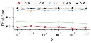
   Figure 11: Finish rate as we vary $b$. Note the x-axis is in log scale.

   Each line in Figure 11 represents the trend of finish rate under a given SLO setting (as a multiple of P99 execution time). And it can be seen that under all SLO settings, ndeed keeps stable finish rate regardless of the choice of $b$. It is therefore safe to choose $b$ to account for floating-point overflow, as we do in s implementation.

   5.7 Overheads

   To understand s scheduling overhead, we evaluate the lower limit on SLOs that an achieve by measuring the finish rate while varying incoming requests’ minimum execution time (time to execute one request alone). In this experiment, we use the same workload with three-modal distribution as shown in 7(c), and scale the whole execution time distribution down until s finish rate drops significantly.

   Figure 12 reports the trends of finish rates under different SLO settings. Similar to other experiments, we set SLOs according to the P99 of minimum execution time and report results under different SLO to P99 ratios from $1.5\times$ to $5\times$. eeps consistent and stable finish rate. Its performance only starts to degrade when the minimum P99 execution time is approaching $20~{}\text{ms}$. At that time, due to variance in request execution time, the mean approaches $10~{}\text{ms}$ and requests can go as low as less than $2~{}\text{ms}$.

   

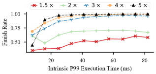
   Figure 12: Finish rate as we vary incoming requests’ minimum execution time.

   6 Related Work

   Model Serving

   We directly compare o Clockwork [18], Nexus [49] and Clipper [10]. While Clockwork’s assumption about static DNNs no longer holds for the dynamic DNNs, its idea of proactively planning ahead and consolidating choices across layers to reduce disturbance still applies in In addition, existing systems propose several orthogonal concepts that can be seen as complementary to Clipper’s idea of model selection and INFaaS’s [43] model variant concept could be applied in front of Nexus’ model prefix-sharing and InferLine’s [9] inference pipelines are also compatible with s idea of tracking request execution time as random variables.

   In cloud or serverless platforms there are projects focusing on serving models at scale [4, 26, 55]. TensorFlow Serving [34] provides one of the first production environments for models trained using the TensorFlow framework. SageMaker [3], Vertex AI [16] and Azure ML [32] are public cloud DNN serving systems that offer developers inference services that auto-scale based on load.

   Cost-Aware Scheduling

   One family of the well-studied scheduling algorithms are cost-aware or utility-based algorithms. The decisions in these algorithms are made to optimize certain costs, which could be defined in many ways: they could be fixed or time-varying values [20, 25], costs of rolling back transactions [23], or derived from SLOs [31, 40, 57]. It is however common in these algorithms to assume the exact execution time to be available during scheduling, which is not the case in serving dynamic DNNs.

   Unknown-Sized Job Scheduling in Cluster

   Scheduling jobs with unknown duration has been studied in cluster computing. 3Sigma [37] uses the job length distribution in the scheduling and enumerates all possible choices to find the optimal scheduling decision. Age-based mechanisms [17, 45] gradually update jobs’ priorities based on sustained service time. There are also various techniques used to mitigate mis-prediction in case the job’s length exceeds expectation [39].

   However, inference request serving differs from the above in its timescale and properties. Inference requests usually complete in less than a second, whereas cluster jobs can last hours or even days. So our scheduler has to make decision very quickly, unlike cluster schedulers that can use extensive searching before settling on a schedule. Furthermore, while cluster jobs are usually preemptable, inference requests are not, which rules out age-based algorithms.

   7 Conclusion

   Dynamic DNNs adapt their structures or parameters to the input, and thus experiencing rapid development thanks to notable advantages in terms of accuracy, computational efficiency, adaptiveness, etc. This challenges existing DNN serving solutions that assume data-independence of incoming requests, and they suffer from poor performance due to the large variance in request execution times. We propose a dynamic DNN serving system, to meet these challenges. aptures the variance in dynamic DNNs by modeling request execution time as random variables, and then efficiently batches and schedules them without knowing a request’s precise execution time. We demonstrated that ignificantly outperforms states-of-the-art serving solutions for high variance dynamic DNN workloads while maintaining nearly identical performance for static workloads.

   While we take a first step in this paper, we hope that ll inspire further research not only on dynamic DNN inference serving systems but other aspects of dynamic DNN lifecycle as well.

   Appendix A Additional Experiment Results

   We report more results in Table 2, Table 3, Table 4, and Table 5.

   Table 2: Evaluation results for cases where request execution time distribution is bimodal. Case ID shows the standard deviation of each modal’s normal distribution.

   Case ID	SLO	Finish Rate
   	($\times$ P99)	Clipper	Nexus	Clockwork
   std-0.5	1.5	0.01	0.01	0.44	0.57
   std-0.5	2	0.01	0.02	0.53	0.76
   std-0.5	3	0.04	0.05	0.62	0.96
   std-0.5	4	0.11	0.13	0.61	0.99
   std-0.5	5	0.20	0.25	0.57	1.00
   std-1	1.5	0.02	0.02	0.46	0.60
   std-1	2	0.03	0.03	0.53	0.76
   std-1	3	0.10	0.10	0.55	0.97
   std-1	4	0.21	0.19	0.53	0.99
   std-1	5	0.33	0.34	0.56	1.00
   std-2	1.5	0.04	0.03	0.43	0.59
   std-2	2	0.07	0.05	0.51	0.73
   std-2	3	0.19	0.13	0.55	0.97
   std-2	4	0.34	0.30	0.50	1.00
   std-2	5	0.49	0.54	0.59	1.00
   std-2/0.5	1.5	0.16	0.18	0.52	0.75
   std-2/0.5	2	0.28	0.32	0.59	0.83
   std-2/0.5	3	0.61	0.68	0.60	0.98
   std-2/0.5	4	0.89	0.93	0.59	0.96
   std-2/0.5	5	0.97	1.00	0.63	1.00
   std-0.5/2	1.5	0.01	0.01	0.38	0.40
   std-0.5/2	2	0.01	0.02	0.50	0.61
   std-0.5/2	3	0.04	0.04	0.57	0.90
   std-0.5/2	4	0.08	0.09	0.66	0.97
   std-0.5/2	5	0.15	0.17	0.52	0.99

   Table 3: Evaluation results for cases where we vary the modality of request execution time distribution.

   Case ID	SLO	Finish Rate
   	($\times$ P99)	Clipper	Nexus	Clockwork
   one-modal	1.5	0.03	0.04	0.48	0.46
   one-modal	2	0.10	0.13	0.55	0.74
   one-modal	3	0.45	0.54	0.61	0.98
   one-modal	4	0.73	0.80	0.58	1.00
   one-modal	5	0.82	0.91	0.60	1.00
   two-modal	1.5	0.01	0.03	0.45	0.60
   two-modal	2	0.04	0.03	0.58	0.75
   two-modal	3	0.13	0.14	0.51	0.97
   two-modal	4	0.27	0.30	0.56	1.00
   two-modal	5	0.37	0.44	0.55	1.00
   three-modal	1.5	0.03	0.04	0.45	0.59
   three-modal	2	0.05	0.05	0.55	0.68
   three-modal	3	0.10	0.09	0.61	0.97
   three-modal	4	0.18	0.23	0.60	0.99
   three-modal	5	0.35	0.42	0.61	0.99
   four-modal	1.5	0.03	0.05	0.46	0.59
   four-modal	2	0.05	0.07	0.56	0.73
   four-modal	3	0.08	0.12	0.59	0.94
   four-modal	4	0.10	0.16	0.60	0.98
   four-modal	5	0.14	0.19	0.60	1.00
   five-modal	1.5	0.02	0.03	0.47	0.60
   five-modal	2	0.02	0.03	0.55	0.73
   five-modal	3	0.03	0.07	0.59	0.94
   five-modal	4	0.04	0.08	0.57	0.97
   five-modal	5	0.07	0.08	0.56	0.99
   six-modal	1.5	0.04	0.04	0.46	0.58
   six-modal	2	0.03	0.05	0.53	0.71
   six-modal	3	0.06	0.08	0.53	0.92
   six-modal	4	0.07	0.09	0.51	0.97
   six-modal	5	0.08	0.11	0.54	0.99
   seven-modal	1.5	0.03	0.05	0.43	0.59
   seven-modal	2	0.04	0.05	0.51	0.73
   seven-modal	3	0.08	0.09	0.54	0.93
   seven-modal	4	0.10	0.12	0.52	0.98
   seven-modal	5	0.12	0.15	0.54	0.99
   eight-modal	1.5	0.03	0.04	0.33	0.60
   eight-modal	2	0.05	0.06	0.49	0.74
   eight-modal	3	0.08	0.09	0.43	0.93
   eight-modal	4	0.09	0.13	0.52	0.97
   eight-modal	5	0.11	0.14	0.50	0.99

   Table 4: Evaluation results for static models.

   Case ID	SLO	Finish Rate
   	($\times$ P99)	Clipper	Nexus	Clockwork
   inception-imagenet	1.5	0.01	0.01	0.16	0.41
   inception-imagenet	2	0.31	0.30	0.58	0.48
   inception-imagenet	3	0.86	0.88	0.84	0.84
   inception-imagenet	4	0.96	0.97	0.82	0.99
   inception-imagenet	5	0.98	0.98	0.83	0.99
   resnet-imagenet	1.5	0.01	0.00	0.30	0.42
   resnet-imagenet	2	0.15	0.15	0.59	0.48
   resnet-imagenet	3	0.62	0.64	0.77	0.85
   resnet-imagenet	4	0.89	0.91	0.88	0.98
   resnet-imagenet	5	0.95	0.96	0.87	0.99

   Table 5: Evaluation results for real tasks. The first part of the case ID is the model name and second part the dataset name.

   Case ID	SLO	Finish Rate
   	($\times$ P99)	Clipper	Nexus	Clockwork
   blenderbot-convAI	1.5	0.05	0.06	0.43	0.45
   blenderbot-convAI	2	0.18	0.21	0.61	0.65
   blenderbot-convAI	3	0.56	0.63	0.64	0.74
   blenderbot-convAI	4	0.71	0.81	0.65	0.81
   blenderbot-convAI	5	0.75	0.87	0.65	0.81
   blenderbot-cornell	1.5	0.06	0.06	0.43	0.44
   blenderbot-cornell	2	0.20	0.20	0.60	0.68
   blenderbot-cornell	3	0.54	0.57	0.62	0.75
   blenderbot-cornell	4	0.71	0.74	0.64	0.81
   blenderbot-cornell	5	0.74	0.77	0.64	0.82
   gpt-convAI	1.5	0.39	0.38	0.39	0.36
   gpt-convAI	2	0.79	0.83	0.57	0.64
   gpt-convAI	3	0.91	0.99	0.61	0.86
   gpt-convAI	4	0.92	1.00	0.63	0.97
   gpt-convAI	5	0.92	1.00	0.61	0.98
   gpt-cornell	1.5	0.45	0.44	0.46	0.44
   gpt-cornell	2	0.84	0.86	0.65	0.68
   gpt-cornell	3	0.94	1.00	0.73	0.97
   gpt-cornell	4	0.94	1.00	0.73	0.99
   gpt-cornell	5	0.95	1.00	0.74	1.00
   bart-cnn	1.5	0.12	0.11	0.44	0.46
   bart-cnn	2	0.36	0.36	0.46	0.71
   bart-cnn	3	0.73	0.73	0.46	0.97
   bart-cnn	4	0.78	0.79	0.44	0.99
   bart-cnn	5	0.80	0.81	0.44	1.00
   t5-cnn	1.5	0.48	0.46	0.47	0.49
   t5-cnn	2	0.86	0.84	0.50	0.74
   t5-cnn	3	0.99	1.00	0.50	1.00
   t5-cnn	4	0.99	1.00	0.52	1.00
   t5-cnn	5	0.99	1.00	0.51	1.00
   fsmt-wmt	1.5	0.04	0.04	0.45	0.45
   fsmt-wmt	2	0.21	0.23	0.50	0.59
   fsmt-wmt	3	0.63	0.65	0.51	0.88
   fsmt-wmt	4	0.73	0.76	0.53	0.93
   fsmt-wmt	5	0.75	0.79	0.54	0.95
   mbart-wmt	1.5	0.07	0.10	0.38	0.47
   mbart-wmt	2	0.28	0.30	0.36	0.59
   mbart-wmt	3	0.71	0.73	0.35	0.91
   mbart-wmt	4	0.76	0.78	0.36	0.96
   mbart-wmt	5	0.78	0.80	0.35	0.98
   rdinet-cifar	1.5	0.61	0.61	0.48	0.49
   rdinet-cifar	2	0.98	0.99	0.47	0.84
   rdinet-cifar	3	0.99	1.00	0.48	1.00
   rdinet-cifar	4	0.99	1.00	0.48	1.00
   rdinet-cifar	5	0.99	1.00	0.48	1.00
   skipnet-imagenet	1.5	0.00	0.00	0.05	0.24
   skipnet-imagenet	2	0.00	0.03	0.14	0.62
   skipnet-imagenet	3	0.00	0.12	0.21	0.92
   skipnet-imagenet	4	0.00	0.31	0.12	0.95
   skipnet-imagenet	5	0.00	0.48	0.16	0.89

   Appendix B Generalization to Piece-wise Step Cost Functions

   We can extend our calculation for Eq. (2) from single-step SLO cost function to multiple-step cost functions. For example, consider a multiple-step cost function with three deadlines $d_{1}$, $d_{2}$ and $d_{3}$, and corresponding costs $c_{1}$, $c_{2}$, $c_{3}$. Such a cost function is actually decomposable into the sum of three single-step cost functions: deadline $d_{1}$ with cost $c1$, deadline $d_{2}$ with cost $c_{2}-c_{1}$, and deadline $d_{3}$ with cost $c_{3}-c_{2}$. Therefore, we can compute the priority score for each of the single-step cost function and sum up the results to get the priority score for the multiple-step cost function.

References

[1]Atul Adya, Daniel Myers, Jon Howell, Jeremy Elson, Colin Meek, Vishesh Khemani, Stefan Fulger, Pan Gu, Lakshminath Bhuvanagiri, Jason Hunter, Roberto Peon, Larry Kai, Alexander Shraer, Arif Merchant and Kfir Lev-Ari
“Slicer: Auto-Sharding for Datacenter Applications”
In 12th USENIX Symposium on Operating Systems Design and Implementation, 2016, pp. 739–753
[2]Alfred V Aho and John E Hopcroft
“The design and analysis of computer algorithms”, 1974
[4]Anirban Bhattacharjee, Ajay Dev Chhokra, Zhuangwei Kang, Hongyang Sun, Aniruddha Gokhale and Gabor Karsai
“Barista: Efficient and scalable serverless serving system for deep learning prediction services”
In IEEE International Conference on Cloud Engineering, 2019, pp. 23–33
IEEE
[5]Ond Bojar, Christian Federmann, Mark Fishel, Yvette Graham, Barry Haddow, Matthias Huck, Philipp Koehn and Christof Monz
“Findings of the 2018 conference on machine translation (wmt18)”
In Proceedings of the Third Conference on Machine Translation2, 2018, pp. 272–307
[6]Rishi Bommasani et al.
“On the Opportunities and Risks of Foundation Models”, 2021
arXiv:2108.07258 [cs.LG]
[7]Yun Chi, Hakan Hacígümüş, Wang-Pin Hsiung and Jeffrey F. Naughton
“Distribution-Based Query Scheduling”
In Proceedings of the VLDB Endowment6.9, 2013, pp. 673–684
[8]Yun Chi, Hyun Jin Moon and Hakan Hacigümüş
“iCBS: incremental cost-based scheduling under piecewise linear SLAs”
In Proceedings of the VLDB Endowment4.9, 2011, pp. 563–574
[9]Daniel Crankshaw, Gur-Eyal Sela, Xiangxi Mo, Corey Zumar, Ion Stoica, Joseph Gonzalez and Alexey Tumanov
“InferLine: latency-aware provisioning and scaling for prediction serving pipelines”
In Proceedings of the 11th ACM Symposium on Cloud Computing, 2020, pp. 477–491
[10]Daniel Crankshaw, Xin Wang, Guilio Zhou, Michael J Franklin, Joseph E Gonzalez and Ion Stoica
“Clipper: A low-latency online prediction serving system”
In 14th USENIX Symposium on Networked Systems Design and Implementation, 2017, pp. 613–627
[11]Cristian Danescu-Niculescu-Mizil and Lillian Lee
“Chameleons in imagined conversations: A new approach to understanding coordination of linguistic style in dialogs”, 2011
arXiv:1106.3077 [cs.CL]
[12]Jacob Devlin, Ming-Wei Chang, Kenton Lee and Kristina Toutanova
“BERT: Pre-training of Deep Bidirectional Transformers for Language Understanding”
In Proceedings of the 2019 Conference of the North American Chapter of the Association for Computational Linguistics: Human Language Technologies, Volume 1 (Long and Short Papers), 2019, pp. 4171–4186
[13]Emily Dinan, Varvara Logacheva, Valentin Malykh, Alexander Miller, Kurt Shuster, Jack Urbanek, Douwe Kiela, Arthur Szlam, Iulian Serban, Ryan Lowe, Shrimai Prabhumoye, Alan W Black, Alexander Rudnicky, Jason Williams, Joelle Pineau, Mikhail Burtsev and Jason Weston
“The Second Conversational Intelligence Challenge (ConvAI2)”, 2019
arXiv:1902.00098 [cs.AI]
[17]Juncheng Gu, Mosharaf Chowdhury, Kang G. Shin, Yibo Zhu, Myeongjae Jeon, Junjie Qian, Hongqiang Harry Liu and Chuanxiong Guo
“Tiresias: A GPU Cluster Manager for Distributed Deep Learning”
In 16th USENIX Symposium on Networked Systems Design and Implementation, 2019, pp. 485–500
[18]Arpan Gujarati, Reza Karimi, Safya Alzayat, Wei Hao, Antoine Kaufmann, Ymir Vigfusson and Jonathan Mace
“Serving DNNs like clockwork: Performance predictability from the bottom up”
In 14th USENIX Symposium on Operating Systems Design and Implementation, 2020, pp. 443–462
[19]Yizeng Han, Gao Huang, Shiji Song, Le Yang, Honghui Wang and Yulin Wang
“Dynamic Neural Networks: A Survey”, 2021
arXiv:2102.04906 [cs.CV]
[20]Jayant R Haritsa, Michael J Canrey and Miron Livny
“Value-based scheduling in real-time database systems”
In The VLDB Journal2.2, 1993, pp. 117–152
[21]Kim Hazelwood, Sarah Bird, David Brooks, Soumith Chintala, Utku Diril, Dmytro Dzhulgakov, Mohamed Fawzy, Bill Jia, Yangqing Jia, Aditya Kalro, James Law, Kevin Lee, Jason Lu, Pieter Noordhuis, Misha Smelyanskiy, Liang Xiong and Xiaodong Wang
“Applied machine learning at Facebook: A datacenter infrastructure perspective”
In IEEE International Symposium on High Performance Computer Architecture, 2018, pp. 620–629
[22]Kaiming He, Xiangyu Zhang, Shaoqing Ren and Jian Sun
“Deep Residual Learning for Image Recognition”, 2015
arXiv:1512.03385 [cs.CV]
[23]D Hong, Theodore Johnson and Sharma Chakravarthy
“Real-time transaction scheduling: A cost conscious approach”
In ACM SIGMOD Record22.2, 1993, pp. 197–206
[24]Ting-Kuei Hu, Tianlong Chen, Haotao Wang and Zhangyang Wang
“Triple Wins: Boosting Accuracy, Robustness and Efficiency Together by Enabling Input-Adaptive Inference”, 2020
arXiv:2002.10025 [cs.CV]
[25]David E Irwin, Laura E Grit and Jeffrey S Chase
“Balancing risk and reward in a market-based task service”
In Proceedings. 13th IEEE International Symposium on High performance Distributed Computing, 2004., 2004, pp. 160–169
IEEE
[26]Ram Srivatsa Kannan, Lavanya Subramanian, Ashwin Raju, Jeongseob Ahn, Jason Mars and Lingjia Tang
“Grandslam: Guaranteeing slas for jobs in microservices execution frameworks”
In Proceedings of the 14th European Conference on Computer Systems, 2019, pp. 1–16
[27]Kate Keahey, Jason Anderson, Zhuo Zhen, Pierre Riteau, Paul Ruth, Dan Stanzione, Mert Cevik, Jacob Colleran, Haryadi S. Gunawi, Cody Hammock, Joe Mambretti, Alexander Barnes, François Halbach, Alex Rocha and Joe Stubbs
“Lessons Learned from the Chameleon Testbed”
In USENIX Annual Technical Conference, 2020
[28]Alex Krizhevsky and Geoffrey Hinton
“Learning multiple layers of features from tiny images”
Citeseer, 2009
[30]Mike Lewis, Yinhan Liu, Naman Goyal, Marjan Ghazvininejad, Abdelrahman Mohamed, Omer Levy, Ves Stoyanov and Luke Zettlemoyer
“BART: Denoising Sequence-to-Sequence Pre-training for Natural Language Generation, Translation, and Comprehension”, 2019
arXiv:1910.13461 [cs.CL]
[31]Zhen Liu, Mark S Squillante and Joel L Wolf
“On maximizing service-level-agreement profits”
In Proceedings of the 3rd ACM conference on Electronic Commerce, 2001, pp. 213–223
[33]Nathan Ng, Kyra Yee, Alexei Baevski, Myle Ott, Michael Auli and Sergey Edunov
“Facebook FAIR’s WMT19 News Translation Task Submission”, 2019
arXiv:1907.06616 [cs.CL]
[34]Christopher Olston, Noah Fiedel, Kiril Gorovoy, Jeremiah Harmsen, Li Lao, Fangwei Li, Vinu Rajashekhar, Sukriti Ramesh and Jordan Soyke
“Tensorflow-Serving: Flexible, high-performance ml serving”, 2017
arXiv:1712.06139 [cs.DC]
[35]Mark H Overmars and Jan Van Leeuwen
“Maintenance of configurations in the plane”
In Journal of computer and System Sciences23, 1981, pp. 166–204
[36]Fahrettin Özbey, Mehmet Güngör and Yunus Bulut
“On distributions of order statistics for nonidentically distributed variables”
In Appl. Math13.1, 2019, pp. 11–16
[37]Jun Woo Park, Alexey Tumanov, Angela Jiang, Michael A. Kozuch and Gregory R. Ganger
“3Sigma: Distribution-Based Cluster Scheduling for Runtime Uncertainty”
In Proceedings of the 13th European Conference on Computer Systems, 2018, pp. 1–17
[38]Jon Michael Peha
“Scheduling and Dropping Algorithms to Support Integrated Services in Packet-Switched Networks”
[39]Yanghua Peng, Yixin Bao, Yangrui Chen, Chuan Wu and Chuanxiong Guo
“Optimus: An Efficient Dynamic Resource Scheduler for Deep Learning Clusters”
In Proceedings of the 13th European Conference on Computer Systems, 2018, pp. 3:1–3:14
[40]Florentina I Popovici and John Wilkes
“Profitable services in an uncertain world”
In Proceedings of the 2005 ACM/IEEE conference on Supercomputing, 2005, pp. 36–36
[41]Colin Raffel, Noam Shazeer, Adam Roberts, Katherine Lee, Sharan Narang, Michael Matena, Yanqi Zhou, Wei Li and Peter J. Liu
“Exploring the Limits of Transfer Learning with a Unified Text-to-Text Transformer”, 2019
arXiv:1910.10683 [cs.LG]
[42]Stephen Roller, Emily Dinan, Naman Goyal, Da Ju, Mary Williamson, Yinhan Liu, Jing Xu, Myle Ott, Kurt Shuster, Eric M. Smith, Y-Lan Boureau and Jason Weston
“Recipes for building an open-domain chatbot”, 2020
arXiv:2004.13637 [cs.CL]
[43]Francisco Romero, Qian Li, Neeraja J. Yadwadkar and Christos Kozyrakis
“INFaaS: A Model-less and Managed Inference Serving System”, 2020
arXiv:1905.13348 [cs.DC]
[44]Olga Russakovsky, Jia Deng, Hao Su, Jonathan Krause, Sanjeev Satheesh, Sean Ma, Zhiheng Huang, Andrej Karpathy, Aditya Khosla, Michael Bernstein, Alexander C. Berg and Li Fei-Fei
“ImageNet Large Scale Visual Recognition Challenge”, 2014
arXiv:1409.0575 [cs.CV]
[45]Ziv Scully, Mor Harchol-Balter and Alan Scheller-Wolf
“SOAP: One Clean Analysis of All Age-Based Scheduling Policies”
In Proceedings of the ACM on Measurement and Analysis of Computing Systems2.1, 2018, pp. 16:1–16:30
[46]Robert Sedgewick
“Left-leaning red-black trees”
In Dagstuhl Workshop on Data Structures17, 2008
[47]Abigail See, Peter J. Liu and Christopher D. Manning
“Get To The Point: Summarization with Pointer-Generator Networks”, 2017
arXiv:1704.04368 [cs.CL]
[48]Mohammad Shahrad, Rodrigo Fonseca, Íñigo Goiri, Gohar Chaudhry, Paul Batum, Jason Cooke, Eduardo Laureano, Colby Tresness, Mark Russinovich and Ricardo Bianchini
“Serverless in the wild: Characterizing and optimizing the serverless workload at a large cloud provider”
In USENIX Annual Technical Conference, 2020, pp. 205–218
[49]Haichen Shen, Lequn Chen, Yuchen Jin, Liangyu Zhao, Bingyu Kong, Matthai Philipose, Arvind Krishnamurthy and Ravi Sundaram
“Nexus: a GPU cluster engine for accelerating DNN-based video analysis”
In Proceedings of the 27th ACM Symposium on Operating Systems Principles, 2019, pp. 322–337
[50]Christian Szegedy, Vincent Vanhoucke, Sergey Ioffe, Jonathon Shlens and Zbigniew Wojna
“Rethinking the Inception Architecture for Computer Vision”, 2015
arXiv:1512.00567 [cs.CV]
[51]Yuqing Tang, Chau Tran, Xian Li, Peng-Jen Chen, Naman Goyal, Vishrav Chaudhary, Jiatao Gu and Angela Fan
“Multilingual Translation with Extensible Multilingual Pretraining and Finetuning”, 2020
arXiv:2008.00401 [cs.CL]
[52]Ashish Vaswani, Noam Shazeer, Niki Parmar, Jakob Uszkoreit, Llion Jones, Aidan N Gomez, Łukasz Kaiser and Illia Polosukhin
“Attention is all you need”
In Advances in Neural Information Processing Systems 30, 2017, pp. 5998–6008
[53]Xin Wang, Fisher Yu, Zi-Yi Dou, Trevor Darrell and Joseph E. Gonzalez
“SkipNet: Learning Dynamic Routing in Convolutional Networks”
In Proceedings of the European Conference on Computer Vision, 2018, pp. 409–424
[54]Carole-Jean Wu, David Brooks, Kevin Chen, Douglas Chen, Sy Choudhury, Marat Dukhan, Kim Hazelwood, Eldad Isaac, Yangqing Jia, Bill Jia, Tommer Leyvand, Hao Lu, Yang Lu, Lin Qiao, Brandon Reagen, Joe Spisak, Fei Sun, Andrew Tulloch, Peter Vajda, Xiaodong Wang, Yanghan Wang, Bram Wasti, Yiming Wu, Ran Xian, Sungjoo Yoo and Peizhao Zhang
“Machine Learning at Facebook: Understanding Inference at the Edge”
In IEEE International Symposium on High Performance Computer Architecture, 2019, pp. 331–344
[55]Chengliang Zhang, Minchen Yu, Wei Wang and Feng Yan
“MArk: Exploiting Cloud Services for Cost-Effective,SLO-Aware Machine Learning Inference Serving”
In USENIX Annual Technical Conference, 2019, pp. 1049–1062
[56]Haoyu Zhang, Ganesh Ananthanarayanan, Peter Bodik, Matthai Philipose, Paramvir Bahl and Michael J. Freedman
“Live Video Analytics at Scale with Approximation and Delay-Tolerance”
In 14th USENIX Symposium on Networked Systems Design and Implementation, 2017, pp. 377–392
[57]Li Zhang and Danilo Ardagna
“SLA based profit optimization in autonomic computing systems”
In Proceedings of the 2nd international conference on Service oriented computing, 2004, pp. 173–182
[58]Yizhe Zhang, Siqi Sun, Michel Galley, Yen-Chun Chen, Chris Brockett, Xiang Gao, Jianfeng Gao, Jingjing Liu and Bill Dolan
“DialoGPT: Large-Scale Generative Pre-training for Conversational Response Generation”, 2019
arXiv:1911.00536 [cs.CL]