Addressing Class Imbalance in Semi-supervised Image Segmentation: A Study on Cardiac MRI

Abstract

Due to the imbalanced and limited data, semi-supervised medical image segmentation methods often fail to produce superior performance for some specific tailed classes. Inadequate training for those particular classes could introduce more noise to the generated pseudo labels, affecting overall learning. To alleviate this shortcoming and identify the under-performing classes, we propose maintaining a confidence array that records class-wise performance during training. A fuzzy fusion of these confidence scores is proposed to adaptively prioritize individual confidence metrics in every sample rather than traditional ensemble approaches, where a set of predefined fixed weights are assigned for all the test cases. Further, we introduce a robust class-wise sampling method and dynamic stabilization for a better training strategy. Our proposed method considers all the under-performing classes with dynamic weighting and tries to remove most of the noises during training. Upon evaluation on two cardiac MRI datasets, ACDC and MMWHS, our proposed method shows effectiveness and generalizability and outperforms several state-of-the-art methods found in the literature.

1 Introduction

Recent years have witnessed a significant improvement in medical image analysis using deep learning tools [5, 4, 8, 6]. In the context of medical imaging, access to large volumes of labelled data is difficult owing to the high cost, required domain-specific expertise, and protracted process involved in generating accurate annotations [7, 3]. Using a lesser amount of training data, on the other hand, significantly affects the model’s performance. To solve this bottleneck, researchers shifted towards the domain of Semi-Supervised Learning (SSL) which exploits unlabeled data information to compensate for the substantial requirement of data annotation [12]. Recently SSL-based medical image segmentation strategies have been widely adopted due to their competing performance and ability to learn from very few annotations. To this end, adversarial learning is a very promising direction where Peng et al. [23] proposed an adversarial co-training strategy to enforce diversity across multiple models. Li et al. [19] took a generative adversarial-based approach for cardiac magnetic resonance imaging (MRI) segmentation, where they proposed utilizing the predictive result as a latent variable to estimate the distribution of the latent. Nie et al. [22] proposed ASDNet, an adversarial attention-based SSL method utilizing a fully convolutional confidence map. Besides, Luo et al. [21] proposed a dual-task consistent network to utilize geometry-aware level-set as well as pixel-level predictions. Contrastive Learning (CL) based strategies [10, 30] have also been instrumental in this purpose by enforcing representations in latent space to be similar for similar representations. Chaitanya et al. [10] showed the effectiveness of global and local contexts to be of utmost importance in contrastive pretraining to mine important latent representations. Lately, Peng et al. [24] tried to address the limitations of these CL-based strategies by proposing a dynamic strategy in CL by adaptively prioritizing individual samples in an unsupervised loss. Other directions involve consistency regularization [29], domain adaptation [28], uncertainty estimation [27], etc.

However, a significant problem to train the existing SSL-based techniques is that they are based on the assumption that every class has an almost equal number of instances [25]. On the contrary, most real-life medical datasets have some classes with notably higher instances in training samples than others, which is technically termed as $class$ $imbalance$. For example, the class $myocardium$ in ACDC [9] is often missing or too small to be detected in apical slices, leading to substandard segmentation performance for this class [9]. This class-wise bias affects the performance of traditional deep learning networks in terms of convergence during the training phase, and generalization on the test set [16].

This paper addresses a relatively new research topic, called the class imbalance problem in SSL-based medical image segmentation. Though explicitly not focusing on class imbalance, our proposed method aims to improvise the segmentation performance of tail classes by keeping track of category-wise confidence scores during training. Furthermore, we incorporate fuzzy adaptive fusion using the Gompertz function where priority is given to individual confidence scores in every sample in this method rather than traditional ensemble approaches (average, weighted average, etc.), where a set of predefined fixed weights is assigned for all the test cases.

2 Proposed Method

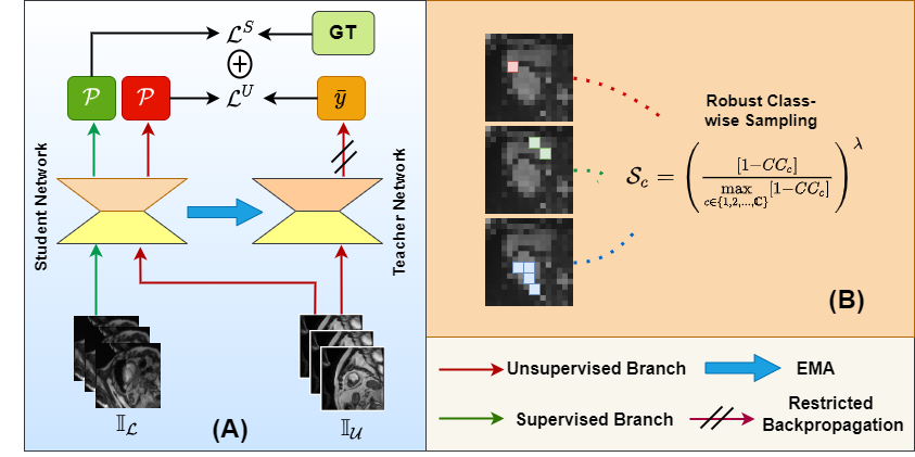
Figure 1: Overall training strategy of the proposed method: (A) the basic student-teacher network, used as a backbone in our work, and (B) the Robust Class-wise Sampling that adaptively samples more pixels from the under-performing classes

Let us assume that the dataset consists of $\mathbb{N}_{1}$ number of labelled images $\mathbb{I}_{\mathcal{L}}$ and $\mathbb{N}_{2}$ number of unlabelled images $\mathbb{I}_{\mathcal{U}}$ (where $\{\mathbb{I}_{\mathcal{L}},\mathbb{I}_{\mathcal{U}}\}\in\mathbb{I}$ and $\mathbb{N}_{1}<<\mathbb{N}_{2}$). First, we define the standard student-teacher architecture, and then formulate our dynamic training strategy by redefining the loss terms.

2.1 Basic Student-Teacher Framework

Similar to [26], our network consists of a student-teacher framework, where the network learns through the student branch only, and the weights of the teacher model are updated by using an Exponential Moving Average (EMA). The student model is used to generate pseudo labels $\bar{\mathcal{Y}}$ on both labelled data $\mathbb{I}_{\mathcal{L}}$ with weak augmentations and unlabelled data $\mathbb{I}_{\mathcal{U}}$ with strong augmentations. In contrast, the teacher model only generates pseudo labels on weakly augmented unlabelled data $\mathbb{I}_{\mathcal{U}}$. The base student-teacher model is shown in Figure 1(A). The standard supervised and unsupervised loss functions ($\mathcal{L}^{S}$ and $\mathcal{L}^{U}$) can, therefore, be defined as:

$$\mathcal{L}^{S}=\frac{1}{\mathbb{N}_{1}}\sum\limits_{n=1}^{\mathbb{N}_{1}}\frac{1}{h\times w}\sum\limits_{i=1}^{h\times w}\mathcal{L}_{CE}(\mathcal{P}_{n,i},GT_{n,i})$$ (1)

$$\mathcal{L}^{U}=\frac{1}{\mathbb{N}_{2}}\sum\limits_{n=1}^{\mathbb{N}_{2}}\frac{1}{h\times w}\sum\limits_{i=1}^{h\times w}\mathcal{L}_{CE}(\mathcal{P}_{n,i},\bar{{y}}_{n,i})$$ (2)

where, $h\times w$ is the image dimension, $\mathcal{L}_{CE}$ represents the standard pixelwise cross-entropy loss, $\mathcal{P}_{n,i}$ represents the prediction of $i^{th}$ pixel of $n^{th}$ image, $GT$ is the ground truth label, and $\bar{y}_{n,i}\in{\bar{\mathcal{Y}}}$ is the generated pseudo label for the corresponding pixel of the corresponding image.

2.2 Dynamic Class-aware Learning

2.2.1 Formulation of Confidence Array

Some of the methods in literature [20, 14] address the imbalanced training in natural scene images by relying on class-wise sample counts followed by ad-hoc weighting and sampling strategies. To this end, we propose maintaining three different performance indicators, namely $Entropy$, $Variance$, and $Confidence$, in a class-wise confidence array to assess the performance of every class. We define $Entropy$ indicator $\mathbb{E}_{c}$ for class $c$ as:

$$\mathbb{E}_{c}=\frac{1}{\mathbb{N}_{1}}\sum\limits_{n=1}^{\mathbb{N}_{1}}\frac{1}{\mathbb{N}_{c}^{n}}\sum\limits_{i=1}^{\mathbb{N}_{c}^{n}}\sum\limits_{j=1}^{\mathbb{C}}\mathcal{P}_{n,i}^{c}\log\mathcal{P}_{n,i}^{j}\>;\>\>\forall c\in\{1,2,3,...,\mathbb{C}\}$$ (3)

where $\mathcal{P}_{n,i}^{j}$ is the $j^{th}$ channel prediction for the $i^{th}$ pixel of $n^{th}$ image. Similarly, we define $Variance$ and $Confidence$ indicators $\mathbb{V}_{c}$ and $\mathbb{C}on_{c}$ respectively as:

$$\begin{split}\mathbb{V}_{c}=\frac{1}{\mathbb{N}_{1}}\sum\limits_{n=1}^{\mathbb{N}_{1}}\frac{1}{\mathbb{N}_{c}^{n}}\sum\limits_{i=1}^{\mathbb{N}_{c}^{n}}\left(\max\limits_{j\in\{1,2,..,\mathbb{C}\}}[\mathcal{P}_{n,i}^{j}]-\mathcal{P}_{n,i}^{c}\right);\>\>\forall c\in\{1,2,3,...,\mathbb{C}\}\end{split}$$ (4)

$$\mathbb{C}on_{c}=\frac{1}{\mathbb{N}_{1}}\sum\limits_{n=1}^{\mathbb{N}_{1}}\frac{1}{\mathbb{N}_{c}^{n}}\sum\limits_{i=1}^{\mathbb{N}_{c}^{n}}\mathcal{P}_{n,i}^{c}\>;\>\>\forall c\in\{1,2,3,...,\mathbb{C}\}$$ (5)

2.2.2 Fuzzy Confidence Fusion

We combine the three class-wise performance indicators $\mathbb{E}_{c}$, $\mathbb{V}_{c}$, and $\mathbb{C}on_{c}$ to generate the final $CC$ score using a fuzzy fusion scheme. Gompertz function was experimentally adopted for fuzzy fusion as explained in the supplementary material. First, we generate a class-wise fuzzy rank of different performance indicators using a re-parameterized Gompertz function [18] as:

$$\mathbb{R}_{c}^{k}=1-e^{-e^{-2\cdot norm(x_{c}^{k})}},\>\>\text{where }x_{c}^{k}\in\{\mathbb{E}_{c},\mathbb{V}_{c},\mathbb{C}on_{c}\},$$ (6)

where, $norm()$ signifies normalization function, $\mathbb{R}_{c}^{k}$ is in range $[0.127,0.632]$, where a higher confidence score gives better (lower) rank. The selection of the objective fuzzy function is based on model performance. For detailed analysis, please refer to the supplementary file. Now, if $M^{k}$ represents top $m$ ranks for class $c$, then we compute a complement of confidence factor sum ($CCF_{c}$) and fuzzy rank sum ($FR_{c}$) as follows:

$$CCF_{c}=\sum_{k}\begin{cases}norm(x_{c}^{k}),&\text{if }\mathbb{R}_{c}^{k}\in M^{k}\\ P_{c}^{CCF},&\text{otherwise }\end{cases}\>\text{and}\>\>FR_{c}=\sum_{k}\begin{cases}\mathbb{R}_{c}^{k},&\text{if }\mathbb{R}_{c}^{k}\in M^{k}\\ P_{c}^{FR},&\text{otherwise }\end{cases}$$ (7)

where, $P_{c}^{CCF}$ and $P_{c}^{FR}$ are the penalty values (set to 0 and 0.632 respectively) for class $c$ to suppress the unlikely winner. The final cumulative confidence ($CC$) score is thereafter computed as:

$$CC_{c}=CCF_{c}\times FR_{c}\>\>\forall c\in\{1,2,...\mathbb{C}\}$$ (8)

The obtained $CC$ score is updated after $t^{\text{th}}$ training iteration as:

$$CC_{c}^{t}\longleftarrow\alpha CC_{c}^{t-1}+(1-\alpha)CC_{c}^{t}\>;\\ \forall c\in\{1,2,3,...,\mathbb{C}\}$$ (9)

where, $\alpha$ is the momentum parameter, set to $0.999$ experimentally.

2.2.3 Robust Class-wise Sampling

We obtain the category-wise confidence score and identify the under-performing classes as described in subsubsection 2.2.1. To alleviate the problem of class-wise training bias, i.e., preventing well-performing classes from overwhelming model training and anchoring the training on a sparse set of under-performing classes, we propose a class-wise sampling rate $\mathcal{S}_{c}$ as:

$$\mathcal{S}_{c}=\left(\frac{[1-CC_{c}]}{\max\limits_{c\in\{1,2,...,\mathbb{C}\}}[1-CC_{c}]}\right)^{\lambda}$$ (10)

where $\lambda$ is a tunable parameter. Instead of sampling all the available pixels for the unsupervised loss formulation, we sample random pixels from class $c$ with sampling rate of $\mathcal{S}_{c}$. So $\mathcal{L}^{U}$ in Equation 2 can be reformulated as:

$$\mathcal{L}^{U}=\frac{1}{\mathbb{N}_{2}}\sum\limits_{n=1}^{\mathbb{N}_{2}}\frac{1}{\left(\sum\limits_{i=1}^{h\times w}\mathds{1}_{n,i}\right)}\sum\limits_{i=1}^{h\times w}\mathds{1}_{n,i}\mathcal{L}_{CE}(\mathcal{P}_{n,i},\bar{{y}}_{n,i})$$ (11)

where $\mathds{1}$ is the binary value operator. The value $\mathds{1}_{n,i}=0$ if the $i^{th}$ pixel from the $n^{th}$ image is not sampled according to sampling rate $\mathcal{S}_{c}$, otherwise set to $1$. Figure 1(B) represents the proposed class-wise sampling strategy.

2.2.4 Dynamic Training Stabilization

As the model performance strictly relies upon the quality of pseudo labels, the under-performing categories insert a significant amount of noise in the pseudo label, hindering the training process. Methods in literature [17] set a higher threshold value to remove the under-performing classes, although this firm criterion leads to lower recall value for those categories, affecting the overall training. We utilize a dynamic modulation of weights to alleviate this problem for better training stabilization. This aims to redistribute the loss contribution from convincing and under-performing samples, i.e., more weights to the convincing classes. The unsupervised loss in Equation 11 can be reformulated as:

$$\mathcal{L}^{U}=\frac{1}{\mathbb{N}_{2}}\sum\limits_{n=1}^{\mathbb{N}_{2}}\frac{1}{\left(\sum\limits_{i=1}^{h\times w}\mathcal{W}_{n,i}\right)}\sum\limits_{i=1}^{h\times w}\mathcal{W}_{n,i}\mathcal{L}_{CE}(\mathcal{P}_{n,i},\bar{{y}}_{n,i})$$ (12)

where $\mathcal{W}_{n,i}$ is the weight provided for the $i^{th}$ pixel in $n^{th}$ image in the final unsupervised loss formulation, and can be defined as:

$$\mathcal{W}_{n,i}=\mathds{1}_{n,i}\max\limits_{c\in\{1,2,...,\mathbb{C}\}}[\mathcal{P}_{n,i}]^{\beta}$$ (13)

where $\beta$ is a tunable parameter. The final loss function is computed as:

$$\mathcal{L}_{total}=\mathcal{L}^{U}+\zeta\mathcal{L}^{S},$$ (14)

where $\zeta$ is a tunable parameter. The value of $\zeta$ decreases with an increase in the number of iterations, limiting the contribution of supervised loss term $\mathcal{L}^{S}$ in the overall loss in the later stage of training.

3 Experiments and Results

3.1 Dataset and Implementation Details

The model is evaluated on two publicly available cardiac MRI datasets. (1) the ACDC dataset [9], hosted in MICCAI17, contains 100 patients’ cardiac MR volumes, where for every patient it has around 15 volumes covering the entire cardiac cycle, and expert annotations for left and right ventricles and myocardium. (2) The MMWHS dataset [31] consists of 20 cardiac MRI samples with expert annotations for seven structures: left and right ventricles, left and right atrium, pulmonary artery, myocardium, and aorta. The datasets are distributed into a $4:1$ ratio of training and validation sets for both cases. To validate the model performance on different label percentages, we use $1.25\%$, $2.5\%$, and $10\%$ labelled data from ACDC and $10\%$, $20\%$, and $40\%$ labelled data from MMWHS for training purposes (label percentage is taken in accordance to other methods in literature). The values of $\beta$ in Equation 13 and $\lambda$ in Equation 10 are taken as $1.5$ and $2.5$, respectively (experimental analysis in supplementary file). The experimentation is implemented using Tesla K80 GPU with 16GB RAM. An SGD optimizer with an initial learning rate $1e-4$, momentum of $0.9$, and weight decay of $0.0001$ was employed. Three widely used metrics are used for the evaluation purpose: Dice Similarity Score (DSC), Average Symmetric Distance (ASD), and Hausdorff Distance (HD) [2].

3.2 Quantitative Performance Evaluation

To empirically illustrate the effective segmentation ability of the proposed model in a semi-supervised environment, we evaluate our proposed method on the ACDC and MMWHS datasets by training the model using different percentages of labelled data (see Figure 2). For the ACDC dataset, the reported DSC, ASD and HD values are 0.746, 0.677, 2.409, respectively while using 1.25$\%$ training samples, 0.842, 0.614, 2.009 corresponding to 2.5$\%$ training labels, 0.889, 0.511, 1.804 for 10$\%$ and 0.902, 0.489, 1.799 while using 100$\%$ samples for training. We consider the 100$\%$ training labels utilization as a fully supervised functioning for comparative analysis. As can be inferred from Figure 2A, the segmentation performance of the proposed model utilizing only a handful of labels is comparable to the fully supervised counterpart. A similar trend is also observed in Figure 2B, where the DSC score while using 10$\%$, 20$\%$, 40$\%$ and 100$\%$ training samples are 0.626, 0.791, 0.815 and 0.826 respectively. The reported ASD scores for the respective cases are 2.397, 1.798, 1.355 and 1.317, respectively. The HD score for the 10$\%$ case is 5.001, which is slightly higher, but while using 40$\%$ of the labels for training, the HD score drops down to 2.221, comparable to the fully supervised case with an HD of 2.183.

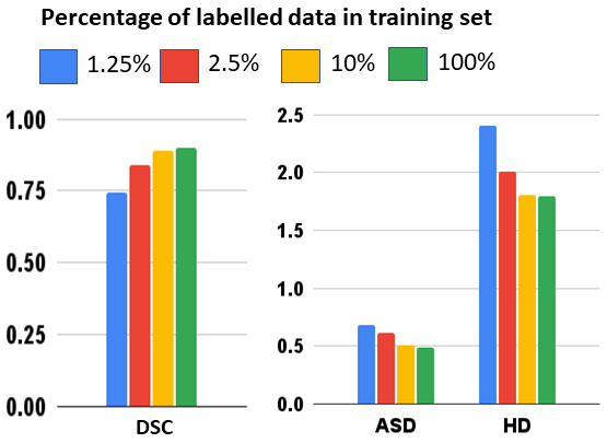
(a) ACDC

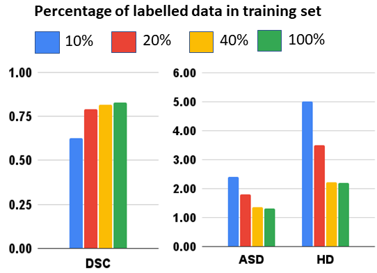
(b) MMWHS

Figure 2: Quantitative segmentation performance of our proposed method using different percentage of labelled data of ACDC and MMWHS.

3.3 Comparison with State-of-the-art

To prove the effectiveness of the proposed model, we have performed its comparative analysis with some state-of-the-art models [13, 15, 12, 11] which is shown in Table 1. As can be inferred, for the ACDC dataset, the average DSC score as reported by our model while using 1.25$\%$ and 2.5$\%$ training samples is the second best with the state-of-the-art performance given by Global + Local CL [10], and PCL [30] respectively. For 10$\%$ training samples, on the other hand, the state-of-the-art performance is reported by the proposed model (DSC=0.889). For the MMWHS dataset, the proposed model surpasses all the existing models in terms of the average DSC score while using 10$\%$, 20$\%$ or 40$\%$ of the training samples, with an average 5$\%$ margin over the second-best performing model. Another important observation is that methods like [30, 1, 15] fail to produce satisfactory results using very few annotations (1.25% and 10% labelled data for ACDC and MMWHS, respectively). In contrast, our proposed method performs quite consistently as compared to those. We record class-wise DSC and sensitivity to observe the improvements for under-performing classes. Observed DSC and sensitivity are (0.934, 0.883, 0.877) and (0.964, 0.925, 0.911) for classes LV, RV, and MYO respectively using 10% labelled data of ACDC. Our method achieves an improvement of $\approx 2-5\%$ for under-performing classes (RV, MYO) than the baseline and literature. Similar improvements are observed across the classes in other experimental settings, both for ACDC and MMWHS.

Table 1: Comparison of the proposed method with state-of-the-art frameworks on ACDC and MMWHS datasets.

Method	Average DSC (ACDC)			Average DSC (MMWHS)
	L=$1.25\%$	L=$2.5\%$	L=$10\%$	L=$10\%$	L=$20\%$	L=$40\%$
Global CL [13]	0.729	-	0.847	0.5	0.659	0.785
PCL [30]	0.671	0.85	0.885	-	-	-
Context Restoration [12]	0.625	0.714	0.851	0.482	0.654	0.783
Label Efficient [15]	-	-	-	0.382	0.553	0.764
Data Aug [11]	0.731	0.786	0.865	0.529	0.661	0.785
Self Train [1]	0.69	0.749	0.86	0.563	0.691	0.801
Global + Local CL [10]	0.757	0.826	0.886	0.617	0.710	0.794
Ours	0.746	0.842	0.889	0.626	0.791	0.815

3.4 Ablation Studies

To find out the potency of different components used in the formulation of our proposed scheme, we perform a detailed ablation study, as shown in Table 2. We use a student-teacher framework as the baseline for all the ablation experiments, which produces an average DSC of $0.819$ and $0.734$ upon evaluation on ACDC and MMWHS datasets, respectively, as a standalone model. Then, we perform two sets of experiments to identify the importance of Robust Class-wise Sampling (RCS) and fuzzy fusion. Instead of fuzzy fusion, as described in Equation 8, first we form the CC score by just simple averaging the three performance indicators: $CC_{c}=(\mathbb{E}_{c}+\mathbb{V}_{c}+\mathbb{C}on_{c})/3$. This, along with the RCS, improves the baseline performance by $4.65\%$ and $6.40\%$ in terms of DSC on ACDc and MMWHS, respectively. To fully utilize the potential of RCS, when we evaluate it along with fuzzy fusion, the model outperforms the baseline DSC by a margin of $6.73\%$ and $7.91\%$ respectively on the two datasets. The fuzzy fusion scheme adaptively prioritizes the confidence scores for individual samples rather than using any preset fixed weights to combine the confidence scores. On the other hand, Dynamic Training Stabilization (DTS) and RCS alleviate the problem of class-wise biased training by adaptively prioritizing the under-performing sample classes. This is also justified by the improvements of $\approx 2\%$ and $\approx 3\%$ on ACDC and MMWHS brought by DTS when used on top of RCS with a simple average rule. Furthermore, we present our proposed scheme using DTS and a fuzzy fusion scheme in RCS to achieve the best DSC of $0.889$ and $0.815$ on ACDC and MMWHS, respectively. Additionally, we also observe the variation of model performance by using three confidence indicators individually (refer to supplementary file).

Table 2: Ablation study to identify the effectiveness of Robust Class-wise Sampling (RCS), Dynamic Training Stabilization (DTS), Fuzzy Fusion on ACDC and MMWHS datasets using 10% and 40% labelled data respectively.

Student-Teacher (Base Model)	RCS		DTS	ACDC			MMWHS
	Simple Avg. Rule	Fuzzy fusion		DSC	ASD	HD	DSC	ASD	HD
✓				0.817	2.697	0.653	0.734	2.898	2.119
✓	✓			0.855	2.118	0.580	0.781	2.419	1.662
✓		✓		0.861	1.978	0.541	0.792	2.328	1.461
✓	✓		✓	0.872	1.893	0.522	0.809	2.291	1.377
✓		✓	✓	0.889	1.804	0.511	0.815	2.221	1.355

4 Conclusion

The scarcity of pixel-level annotations has always been a significant hurdle for medical image segmentation. Besides, a limitation of the deep-learning-based strategies is that they get biased toward the majority class, thereby affecting the overall model performance. To this end, our work addresses both issues by forming a class-wise performance-aware dynamic learning strategy. Experimentation on two publicly available cardiac MRI datasets exhibits the superiority of the proposed method over the state-of-the-art methods. In future, we plan to extend the work by designing it as a fine-tuning strategy on top of a contrastive pre-training for more effective utilization of the global context.

References

- [1] Bai, W., Oktay, O., Sinclair, M., Suzuki, H., Rajchl, M., Tarroni, G., Glocker, B., King, A., Matthews, P.M., Rueckert, D.: Semi-supervised learning for network-based cardiac mr image segmentation. In: International Conference on Medical Image Computing and Computer-Assisted Intervention. pp. 253–260. Springer (2017)
- [2] Basak, H., Bhattacharya, R., Hussain, R., Chatterjee, A.: An embarrassingly simple consistency regularization method for semi-supervised medical image segmentation. arXiv preprint arXiv:2202.00677 (2022)
- [3] Basak, H., Bhattacharya, R., Hussain, R., Chatterjee, A.: An exceedingly simple consistency regularization method for semi-supervised medical image segmentation. In: 2022 IEEE 19th International Symposium on Biomedical Imaging (ISBI). pp. 1–4. IEEE (2022)
- [4] Basak, H., Hussain, R., Rana, A.: Dfenet: A novel dimension fusion edge guided network for brain mri segmentation. SN Computer Science 2(6), 1–11 (2021)
- [5] Basak, H., Kundu, R.: Comparative study of maturation profiles of neural cells in different species with the help of computer vision and deep learning. In: International Symposium on Signal Processing and Intelligent Recognition Systems. pp. 352–366. Springer (2020)
- [6] Basak, H., Kundu, R., Chakraborty, S., Das, N.: Cervical cytology classification using pca and gwo enhanced deep features selection. SN Computer Science 2(5), 1–17 (2021)
- [7] Basak, H., Kundu, R., Sarkar, R.: Mfsnet: A multi focus segmentation network for skin lesion segmentation. Pattern Recognition 128, 108673 (2022)
- [8] Basak, H., Rana, A.: F-unet: A modified u-net architecture for segmentation of stroke lesion. In: International Conference on Computer Vision and Image Processing. pp. 32–43. Springer (2020)
- [9] Bernard, O., Lalande, A., Zotti, C., Cervenansky, F., Yang, X., Heng, P.A., Cetin, I., Lekadir, K., Camara, O., Ballester, M.A.G., et al.: Deep learning techniques for automatic mri cardiac multi-structures segmentation and diagnosis: is the problem solved? IEEE transactions on medical imaging 37(11), 2514–2525 (2018)
- [10] Chaitanya, K., Erdil, E., Karani, N., Konukoglu, E.: Contrastive learning of global and local features for medical image segmentation with limited annotations. arXiv preprint arXiv:2006.10511 (2020)
- [11] Chaitanya, K., Karani, N., Baumgartner, C.F., Becker, A., Donati, O., Konukoglu, E.: Semi-supervised and task-driven data augmentation. In: International conference on information processing in medical imaging. pp. 29–41. Springer (2019)
- [12] Chen, L., Bentley, P., Mori, K., Misawa, K., Fujiwara, M., Rueckert, D.: Self-supervised learning for medical image analysis using image context restoration. Medical image analysis 58, 101539 (2019)
- [13] Chen, T., Kornblith, S., Norouzi, M., Hinton, G.: A simple framework for contrastive learning of visual representations. In: International conference on machine learning. pp. 1597–1607. PMLR (2020)
- [14] Hu, H., Wei, F., Hu, H., Ye, Q., Cui, J., Wang, L.: Semi-supervised semantic segmentation via adaptive equalization learning. Advances in Neural Information Processing Systems 34 (2021)
- [15] Hu, X., Zeng, D., Xu, X., Shi, Y.: Semi-supervised contrastive learning for label-efficient medical image segmentation. In: International Conference on Medical Image Computing and Computer-Assisted Intervention. pp. 481–490. Springer (2021)
- [16] Japkowicz, N., Stephen, S.: The class imbalance problem: A systematic study. Intelligent data analysis 6(5), 429–449 (2002)
- [17] Ke, Z., Qiu, D., Li, K., Yan, Q., Lau, R.W.: Guided collaborative training for pixel-wise semi-supervised learning. In: Computer Vision–ECCV 2020: 16th European Conference, Glasgow, UK, August 23–28, 2020, Proceedings, Part XIII 16. pp. 429–445. Springer (2020)
- [18] Kundu, R., Basak, H., Singh, P.K., Ahmadian, A., Ferrara, M., Sarkar, R.: Fuzzy rank-based fusion of cnn models using gompertz function for screening covid-19 ct-scans. Scientific reports 11(1), 1–12 (2021)
- [19] Li, S., Zhang, Y., Yang, X.: Semi-supervised cardiac mri segmentation based on generative adversarial network and variational auto-encoder. In: 2021 IEEE International Conference on Bioinformatics and Biomedicine (BIBM). pp. 1402–1405. IEEE (2021)
- [20] Li, Y., Wang, T., Kang, B., Tang, S., Wang, C., Li, J., Feng, J.: Overcoming classifier imbalance for long-tail object detection with balanced group softmax. In: Proceedings of the IEEE/CVF conference on computer vision and pattern recognition. pp. 10991–11000 (2020)
- [21] Luo, X., Chen, J., Song, T., Wang, G.: Semi-supervised medical image segmentation through dual-task consistency. In: Proceedings of the AAAI Conference on Artificial Intelligence. vol. 35, pp. 8801–8809 (2021)
- [22] Nie, D., Gao, Y., Wang, L., Shen, D.: Asdnet: Attention based semi-supervised deep networks for medical image segmentation. In: International conference on medical image computing and computer-assisted intervention. pp. 370–378. Springer (2018)
- [23] Peng, J., Estrada, G., Pedersoli, M., Desrosiers, C.: Deep co-training for semi-supervised image segmentation. Pattern Recognition 107, 107269 (2020)
- [24] Peng, J., Wang, P., Desrosiers, C., Pedersoli, M.: Self-paced contrastive learning for semi-supervised medical image segmentation with meta-labels. Advances in Neural Information Processing Systems 34 (2021)
- [25] Stanescu, A., Caragea, D.: Semi-supervised self-training approaches for imbalanced splice site datasets. In: Proceedings of The Sixth International Conference on Bioinformatics and Computational Biology, BICoB 2014. pp. 131–136 (2014)
- [26] Tarvainen, A., Valpola, H.: Mean teachers are better role models: Weight-averaged consistency targets improve semi-supervised deep learning results. arXiv preprint arXiv:1703.01780 (2017)
- [27] Wang, K., Zhan, B., Zu, C., Wu, X., Zhou, J., Zhou, L., Wang, Y.: Tripled-uncertainty guided mean teacher model for semi-supervised medical image segmentation. In: International Conference on Medical Image Computing and Computer-Assisted Intervention. pp. 450–460. Springer (2021)
- [28] Xia, Y., Yang, D., Yu, Z., Liu, F., Cai, J., Yu, L., Zhu, Z., Xu, D., Yuille, A., Roth, H.: Uncertainty-aware multi-view co-training for semi-supervised medical image segmentation and domain adaptation. Medical Image Analysis 65, 101766 (2020)
- [29] Xie, Y., Zhang, J., Liao, Z., Verjans, J., Shen, C., Xia, Y.: Intra-and inter-pair consistency for semi-supervised gland segmentation. IEEE Transactions on Image Processing 31, 894–905 (2021)
- [30] Zeng, D., Wu, Y., Hu, X., Xu, X., Yuan, H., Huang, M., Zhuang, J., Hu, J., Shi, Y.: Positional contrastive learning for volumetric medical image segmentation. In: International Conference on Medical Image Computing and Computer-Assisted Intervention. pp. 221–230. Springer (2021)
- [31] Zhuang, X., Shen, J.: Multi-scale patch and multi-modality atlases for whole heart segmentation of mri. Medical image analysis 31, 77–87 (2016)