Supervised Contrastive Learning with Hard Negative Samples

Abstract

Unsupervised contrastive learning (UCL) is a self-supervised learning technique that aims to learn a useful representation function by pulling positive samples close to each other while pushing negative samples far apart in the embedding space. To improve the performance of UCL, several works introduced hard-negative unsupervised contrastive learning (H-UCL) that aims to select the “hard" negative samples in contrast to a random sampling strategy used in UCL. In another approach, under the assumption that the label information is available, supervised contrastive learning (SCL) has developed recently by extending the UCL to a fully-supervised setting. In this paper, motivated by the effectiveness of hard-negative sampling strategies in H-UCL and the usefulness of label information in SCL, we propose a contrastive learning framework called hard-negative supervised contrastive learning (H-SCL). Our numerical results demonstrate the effectiveness of H-SCL over both SCL and H-UCL on several image datasets. In addition, we theoretically prove that, under certain conditions, the objective function of H-SCL can be bounded by the objective function of H-UCL but not by the objective function of UCL. Thus, minimizing the H-UCL loss can act as a proxy to minimize the H-SCL loss while minimizing UCL loss cannot. As we numerically showed that H-SCL outperforms other contrastive learning methods, our theoretical result (bounding H-SCL loss by H-UCL loss) helps to explain why H-UCL outperforms UCL in practice.

1 Introduction

Unsupervised (or self-supervised) contrastive learning (UCL) has received more attention over recent years due to its applications ranging from image classification Tian et al. (2020a); Chen et al. (2020), text classification Pan et al. (2022); Chen et al. (2022), natural language processing Zhang et al. (2022b); Rethmeier and Augenstein (2021) to learning from time-series data Mohsenvand et al. (2020); Nonnenmacher et al. (2022). UCL is a machine learning technique that aims to learn useful representation features from unlabeled datasets by teaching the model which data points are similar or different from each other. For a given sample called “anchor", the similar sample is called the “positive" sample while the different sample is called the “negative" sample. Since no labels are available in UCL settings, positive samples are usually constructed via data augmentations of the given anchor while negative samples are formed by randomly selecting other samples from the same mini-batch. By pulling the anchor and the positive sample close to each other while pushing apart the anchor and the negative sample in embedding space, UCL can learn a low-dimensional representation of data that can be subsequently used in the downstream tasks.

In UCL the negative sampling distribution can have significant impact on the learned representation and performance in downstream tasks. Recent works Robinson et al. (2020); Tabassum et al. (2022) have focused on using “hard" negative samples, i.e., the negative samples that are difficult to distinguish from the anchor, to improve performance. It is well-known that hard-negative unsupervised contrastive learning (H-UCL) outperforms the traditional UCL in practice Robinson et al. (2020); Tabassum et al. (2022), but there is no rigorous theoretical explanation available that satisfactorily explains the empirical findings.

In contrast to UCL and H-UCL which are both unsupervised learning techniques, supervised contrastive learning (SCL) Khosla et al. (2020) has developed recently which extends UCL to a fully-supervised setting where label information us used to select the positive and negative samples. Due to the additional label information, SCL can achieve higher performance than UCL Khosla et al. (2020).

Figure 1: Top-1 accuracy (in %) of UCL, H-UCL, SCL, and H-SCL on CIFAR100 dataset.

In this paper, our contribution is three-fold:

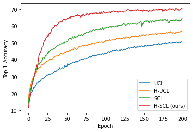
1. Motivated by the hard-negative sampling strategies in H-UCL and the use of label information in SCL, we propose a new framework called hard-negative supervised contrastive learning (H-SCL) which utilizes both hard sampling strategies and label information to improve the performance of learning models. The objective function of H-SCL is simple to implement and available at this link. We numerically show that H-SCL outperforms both SCL and H-UCL on three image datasets. Figure 1 illustrates the performance of H-SCL compared to other methods on the CIFAR100 dataset. More numerical results are provided later in Sec. 6.

2. We theoretically show that, under certain conditions, the H-SCL loss can be bounded by H-UCL loss but not by the UCL loss. Therefore, optimizing the H-UCL loss can be interpreted as proxy for optimizing the H-SCL loss. Since H-SCL practically outperforms other contrastive learning methods, our theoretical results provide an appealing explanation for the good empirical performance of H-UCL over UCL.

3. The UCL, H-UCL, SCL, and H-SCL methods were all separately proposed at different times with different conventions and notation. Our last contribution is a unified presentation that quickly and clearly summarizes these different methods. This not only provides a comprehensive view of the state-of-the-art contrastive learning frameworks but also helps to clearly identify the connections between them, especially their similarities and differences.

The remainder of this paper is structured as follows. In Sec. 2, we summarize the recent works on contrastive learning under UCL, H-UCL, and SCL settings. Sec. 3 formally defines the problem and clarifies the notations. Section 4 describes in detail the settings of H-SCL which is the first contribution of this paper. Section 5 characterizes the relationship between the loss functions of H-UCL and H-SCL which is the second contribution of this paper. Finally, we provide numerical results in Sec. 6 and conclude in Sec. 7.

2 Related work

Unsupervised contrastive learning Chopra et al. (2005); Hadsell et al. (2006) is one of the most popular unsupervised methods for learning representations Oord et al. (2018); Tian et al. (2020a); Chen et al. (2020). UCL aims to find a representation map such that the anchor and its positive sample are pulled closer while the anchor and its negative samples are pushed far away in the latent space. Various frameworks for contrastive learning have been proposed over the past decade, for example, SimCLR Chen et al. (2020) which uses augmented of other images in the same mini-batch as the negative samples, and MoCo He et al. (2020) which uses extra memory to recall the previous negative samples to enable the use of a very large batch of negative samples. Beyond computer vision applications such as image or video representation learning Tian et al. (2020a); Chen et al. (2020); Liu et al. (2021); Wang et al. (2021); Sun et al. (2022); Pang et al. (2022); Yang et al. (2022); Zhang et al. (2022b); Liang et al. (2022); Kim and Song (2021); Yao et al. (2022), UCL has applied for text classification Pan et al. (2022); Chen et al. (2022); Zhang et al. (2022a); Liu et al. (2022), natural language processing Zhang et al. (2022b); Rethmeier and Augenstein (2021); Ye et al. (2021), document summarization Shi et al. (2019), graph You et al. (2020); Wan et al. (2021); Fang et al. (2022); Mo et al. (2022); Yu et al. (2022); Yin et al. (2022), remote sensing Bjorck et al. (2021), aspect detection Shi et al. (2021), online clustering Li et al. (2021), and time-series signals Mohsenvand et al. (2020); Nonnenmacher et al. (2022).

Supervised contrastive learning (SCL) Khosla et al. (2020) has developed recently which extended the unsupervised contrastive learning (UCL) approach to the fully-supervised setting, i.e., using the label information to select the positive and negative samples. There is also an approach called semi-supervised contrastive learning which partially uses label information to enhance the learning capability Zhai et al. (2019); Wu et al. (2018); Henaff (2020). Due to the additional information from the label, it has observed that SCL achieves higher performance than UCL in practice Khosla et al. (2020).

Because the strategy of selecting positive and negative samples is important in UCL Wu et al. (2017); Yuan et al. (2017), several works aim to design better strategies for selecting positive and negative samples. Chen et al. Chen et al. (2020) are based on the perturbations of images to generate positive samples. Tian et al. Tian et al. (2020b) want to select the positive samples such that the mutual information between the anchor and the positive samples is minimized. For negative samples selection, recent works focus on designing “hard" negative samples, i.e., the negative samples coming from different classes with the anchor but close to the anchor. Robinson et al. Robinson et al. (2020) derive a simple but practical hard-negative sampling strategy that improves the downstream task performance on image, graph, and text data. Tabassum et al. Tabassum et al. (2022) introduce an algorithm called UnReMix which takes into account both the anchor similarity and the model uncertainty to select hard negative samples. Kalantidis et al. Kalantidis et al. (2020) propose a method called “hard negative mixing" which synthesizes hard negative samples directly in the embedding space to improve the downstream-task performances. Although many studies observed that H-UCL outperforms UCL, there is no theoretical justification for this observation. Specifically, Wu et al. Wu et al. (2020) pointed out that compared to UCL loss, H-UCL loss is, indeed, a looser lower bound of mutual information between two random variables derived from the dataset and raises the question “why is a looser bound ever more useful" in practice?

In this paper, to utilize the advantages of hard-negative sampling strategies and label information, we propose a framework called hard-negative supervised contrastive learning (H-SCL). To the best of our knowledge, this paper is the first one that jointly combines the label information and the hard-negative sampling strategies to improve learning performance. Our numerical results show that H-SCL outperforms other contrastive learning methods such as SCL, UCL, and H-UCL. In addition, our theoretical result can be used to answer the question raised by Wu et al. Wu et al. (2020) by theoretically proving the usefulness of H-UCL over UCL.

3 Problem formulation

Figure 2: Schematic illustration of negative sampling strategies under H-UCL, SCL, and H-SCL settings in classifying species of cat. Top row (SCL): the negative samples (red rings) are randomly sampled from the set of circle samples which belongs to different classes of the anchor (yellow triangle). Middle row (H-UCL): the negative samples (red rings) are only selected from the neighbors of the anchor (yellow triangle). Since H-UCL prefers samples that are close to the anchor, it may select false negative samples (green triangles) which come from the same class as the anchor. Bottom row (H-SCL): the negative samples (red rings) are selected such that they are not only the true negative samples (circle samples) but also are close to the anchor (yellow triangle).

3.1 Notations

Contrastive learning assumes access to similar data pairs $(v,v^{+})$ of anchor $v$ and positive sample $v^{+}$ that come from a (positive) distribution $p$, i.e., $(v,v^{+})\sim p(v,v^{+})$ as well as $k$ i.i.d. negative samples $v_{1}^{-},v_{2}^{-},\dots,v_{k}^{-}$ from a (negative) distribution $q$ that are presumably unrelated to $v$, $v_{j}^{-}\sim q$, $j=1,2,\dots,k$. Let $\mathcal{C}$ denote the set of all latent classes. Associated with each class $c\in\mathcal{C}$ is a probability distribution $\mathcal{D}_{c}$ over input space $\mathcal{X}$. We use $\rho$ to denote the distribution of classes in dataset.

Let $y:\mathcal{X}\rightarrow\mathcal{Y}$ is a labeling function from the input space to the label space. For an input $w\in\mathcal{X}$, $y(w)$ represents the label of $w$ which is known under supervised settings (SCL, H-SCL), but is unknown under unsupervised settings (UCL, H-UCL).

Learning process is done over $\mathcal{F}$, a class of representation functions $f$ that map from the input space to the latent space $f:\mathcal{X}\rightarrow\mathcal{R}^{d}$.

For a sample $w\sim\mathcal{D}_{c}$ and a set $\mathcal{A}$, let:

$$\mathcal{D}_{c}(\mathcal{A})=\mathbb{E}_{w\sim\mathcal{D}_{c}}[\mathbb{1}(w\in\mathcal{A})]$$ (1)

where $\mathbb{E}$ denotes the expectation and $\mathbb{1}(w\in\mathcal{A})=1$ if $w\in\mathcal{A}$ and $\mathbb{1}(w\in\mathcal{A})=0$, otherwise.

Finally, we define:

$$\mathcal{D}_{c}(w|\mathcal{A})=\begin{cases}\dfrac{\mathcal{D}_{c}(w)}{\mathcal{D}_{c}(\mathcal{A})},&\textup{ if }w\in\mathcal{A},\\ 0&\textup{ otherwise.}\end{cases}$$ (2)

3.2 UCL, H-UCL and SCL settings

We assume that the positive pair $(v,v^{+})$ is i.i.d. selected from the same class distribution $\mathcal{D}_{c}$ for some class $c$ picked randomly according to measure $\rho$:

$$p(v,v^{+})=\mathbb{E}_{c\sim\rho}\leavevmode\nobreak\ \mathcal{D}_{c}(v)\leavevmode\nobreak\ \mathcal{D}_{c}(v^{+}).$$ (3)

For a given $(v,v^{+})$, the main difference between UCL, SCL, and H-UCL comes from the negative distribution $q$ which depends on sampling strategies.

1. Under UCL settings, the negative distribution $q=q_{\textup{\tiny UCL}}$ is:

   $$q_{\textup{\tiny UCL}}(v_{j}^{-})=\mathbb{E}_{c\sim\rho}\leavevmode\nobreak\ \mathcal{D}_{c}(v_{j}^{-}).$$ (4)

   In other words, under UCL settings, the negative samples can be selected from the entire input space $\mathcal{X}$. We use $\mathcal{H}_{\textup{\tiny UCL}}(v)$ to denote set of negative samples for a given $v$ under UCL settings.

2. Under H-UCL settings, for given $v$ and representation function $f\in\mathcal{F}$, let $\mathcal{H}_{\textup{\tiny H-UCL}}(v,f,\tau)$ denote the set of hard-negative samples under unsupervised setting:

   $$\mathcal{H}_{\textup{\tiny H-UCL}}(v,f,\tau)=\big{\{}w\in\mathcal{X}|e^{g(v,w)}\geq\tau\big{\}}$$ (5)

   where $g(a,b)=(f^{T}(a)\cdot f(b))/\gamma$, $\cdot$ denotes the inner (dot) product, $\gamma$ is a positive scalar temperature parameter, and $\tau$ is a positive threshold that controls the hardness of sampling strategies. A larger value of $\tau$, a harder of distinguishing between $v$ and $w$. Note that different values of $\tau$ can be used for different choices of $v$ and $f$.

   Under H-UCL settings, the negative distribution $q=q_{\textup{\tiny H-UCL}}$ is:

   $$q_{\textup{\tiny H-UCL}}(v_{j}^{-})=\mathbb{E}_{c\sim\rho}\leavevmode\nobreak\ \mathcal{D}_{c}(v_{j}^{-}|\mathcal{H}_{\textup{\tiny H-UCL}}(v,f,\tau))$$ (6)

   where $\mathcal{D}_{c}(\cdot|\cdot)$ is defined in (2). In other words, under H-UCL settings, we only pick the negative sample $v_{j}^{-}$ from $\mathcal{H}_{\textup{\tiny H-UCL}}(v,f,\tau)$ where $e^{g(v,v_{j}^{-})}\geq\tau$.

3. Under SCL settings, for a given $v$ with its corresponding label $y(v)$, let $\mathcal{H}_{\textup{\tiny SCL}}$ denote the set of samples having different labels (classes) with $v$. Formally:

   $$\mathcal{H}_{\textup{\tiny SCL}}(v)=\big{\{}w\in\mathcal{X}\,|\,y(w)\neq y(v)\big{\}}.$$ (7)

   Then the negative distribution $q=q_{\textup{\tiny SCL}}$ is:

   $$q_{\textup{\tiny SCL}}(v_{j}^{-})=\mathbb{E}_{c\sim\rho}\leavevmode\nobreak\ \mathcal{D}_{c}(v_{j}^{-}|\mathcal{H}_{\textup{\tiny SCL}}(v)).$$ (8)

   In other words, under SCL settings, we only select the negative samples $v_{j}^{-}$ from $\mathcal{H}_{\textup{\tiny SCL}}(v)$ which is the set of samples having different labels with $v$.

Finally, to shorten the notations, we denote $k$ negative samples $v_{1}^{-},v_{2}^{-},\dots,v_{k}^{-}$ by $v_{1:k}^{-}$, and define:

$$\Psi(v,v^{+},v_{1:k}^{-},f)\!=\!-\log\!\Bigg{[}\dfrac{e^{g(v,v^{+})}}{e^{g(v,v^{+})}+\dfrac{1}{k}\sum_{j=1}^{k}e^{g(v,v_{j}^{-})}}\Bigg{]}.$$ (9)

Given the above settings, let:

1. $\mathcal{L}_{\textup{\tiny UCL}}$ denote the contrastive loss under UCL settings:

   $$\mathcal{L}_{\textup{\tiny UCL}}=\mathbb{E}_{v,v^{+}\sim p}\,\mathbb{E}_{v_{1:k}^{-}\sim q_{\textup{\tiny UCL}}}\Big{[}\Psi(v,v^{+},v_{1:k}^{-},f)\Big{]}.$$ (10)

2. $\mathcal{L}_{\textup{\tiny H-UCL}}$ denote the contrastive loss under H-UCL settings:

   $$\mathcal{L}_{\textup{\tiny H-UCL}}=\mathbb{E}_{v,v^{+}\sim p}\,\mathbb{E}_{v_{1:k}^{-}\sim q_{\textup{\tiny H-UCL}}}\Big{[}\Psi(v,v^{+},v_{1:k}^{-},f)\Big{]}.$$ (11)

3. $\mathcal{L}_{\textup{\tiny SCL}}$ denote the contrastive loss under SCL settings:

   $$\mathcal{L}_{\textup{\tiny SCL}}=\mathbb{E}_{v,v^{+}\sim p}\,\mathbb{E}_{v_{1:k}^{-}\sim q_{\textup{\tiny SCL}}}\Big{[}\Psi(v,v^{+},v_{1:k}^{-},f)\Big{]}.$$ (12)

It is worth noting that the definitions of $\mathcal{L}_{\textup{\tiny UCL}}$, $\mathcal{L}_{\textup{\tiny H-UCL}}$, and $\mathcal{L}_{\textup{\tiny SCL}}$ are already introduced in previous works Robinson et al. (2020); Khosla et al. (2020). Next, hard-negative supervised contrastive learning (H-SCL) will be introduced in Sec. 4 which is the first contribution of this paper.

4 Hard-negative supervised contrastive learning (H-SCL)

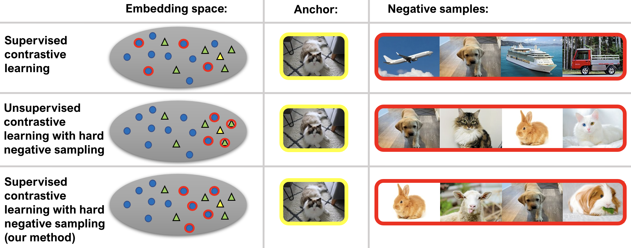
Motivated by the effectiveness of hard-negative sampling strategies in H-UCL and the usefulness of label information in SCL, we propose a learning framework called hard-negative supervised contrastive learning (H-SCL) which utilizes both the hard-negative sampling schemes and the label information to improve the learning performance. The main difference between H-SCL and other contrastive learning methods (UCL, H-UCL, and SCL) comes from the way the negative samples are selected.

Formally, in H-SCL, the positive pair $(v,v^{+})$ is first sampled using Eq. (3), i.e., using the same sampling strategy as UCL, H-UCL, and SCL. Next, for given positive pair $(v,v^{+})$, label $y(v)$, representation function $f$, and threshold $\tau$, the negative distribution $q=q_{\textup{\tiny H-SCL}}$ is:

$$q_{\textup{\tiny H-SCL}}(v_{j}^{-})=\mathbb{E}_{c\sim\rho}\leavevmode\nobreak\ \mathcal{D}_{c}(v_{j}^{-}|\mathcal{H}_{\textup{\tiny H-SCL}}(v,f,\tau)),$$ (13)

where

$$\mathcal{H}_{\textup{\tiny H-SCL}}(v,f,\tau)=\mathcal{H}_{\textup{\tiny SCL}}(v)\cap\mathcal{H}_{\textup{\tiny H-UCL}}(v,f,\tau).$$ (14)

In other words, under H-SCL settings, we only select the negative sample $v_{j}^{-}$ which simultaneously satisfies:

1. $v_{j}^{-}$ has a different label with $v$, i.e., $v_{j}^{-}\in\mathcal{H}_{\textup{\tiny SCL}}$, and

2. $v_{j}^{-}$ is hard to discern from $v$, i.e., $v_{j}^{-}\in\mathcal{H}_{\textup{\tiny H-UCL}}$, $e^{g(v,v_{j}^{-})}\geq\tau$.

Finally, recall that $p$ denotes the distribution of positive pairs $(v,v^{+})$, $v_{1:k}^{-}$ denotes $k$ negative samples, $f$ denotes the representation function, $q_{\textup{\tiny H-SCL}}$ denotes the negative distribution of samples sampled from $\mathcal{H}_{\textup{\tiny H-SCL}}$, and $\Psi(v,v^{+},v_{1:k}^{-},f)$ is defined in Eq. (9), then the loss function under hard-negative supervised contrastive learning (H-SCL) settings is:

$$\mathcal{L}_{\textup{\tiny H-SCL}}=\mathbb{E}_{v,v^{+}\sim p}\,\mathbb{E}_{v_{1:k}^{-}\sim q_{\textup{\tiny H-SCL}}}\Big{[}\Psi(v,v^{+},v_{1:k}^{-},f)\Big{]}.$$ (15)

The top row, middle row, and bottom row in Fig. 2 illustrate the negative sampling strategies in SCL, H-UCL, and H-SCL, respectively. In Sec. 6, we numerically demonstrate the advantages of H-SCL against SCL, UCL, and H-UCL.

5 Connection between H-SCL loss and H-UCL loss

In this section, we will show that the loss function under hard-negative supervised contrastive learning settings ($\mathcal{L}_{\textup{\tiny H-SCL}}$) is upper bounded by the loss function under hard-negative unsupervised contrastive learning settings ($\mathcal{L}_{\textup{\tiny H-UCL}}$) under some certain conditions, i.e., showing that $\mathcal{L}_{\textup{\tiny H-SCL}}\leq\mathcal{L}_{\textup{\tiny H-UCL}}$. This together with, in general, there is no relationship between the loss function under hard-negative supervised contrastive learning settings ($\mathcal{L}_{\textup{\tiny H-SCL}}$) and the loss function under unsupervised contrastive learning settings ($\mathcal{L}_{\textup{\tiny UCL}}$) leads to our conclusion that minimizing $\mathcal{L}_{\textup{\tiny H-UCL}}$ can act as a proxy to minimize $\mathcal{L}_{\textup{\tiny H-SCL}}$ while minimizing $\mathcal{L}_{\textup{\tiny UCL}}$ cannot. Because H-SCL empirically outperforms other contrastive learning methods (see Sec. 6), our theoretical results suggest a way to explain why H-UCL outperforms UCL in practice which answers the question of Wu et al. Wu et al. (2020).

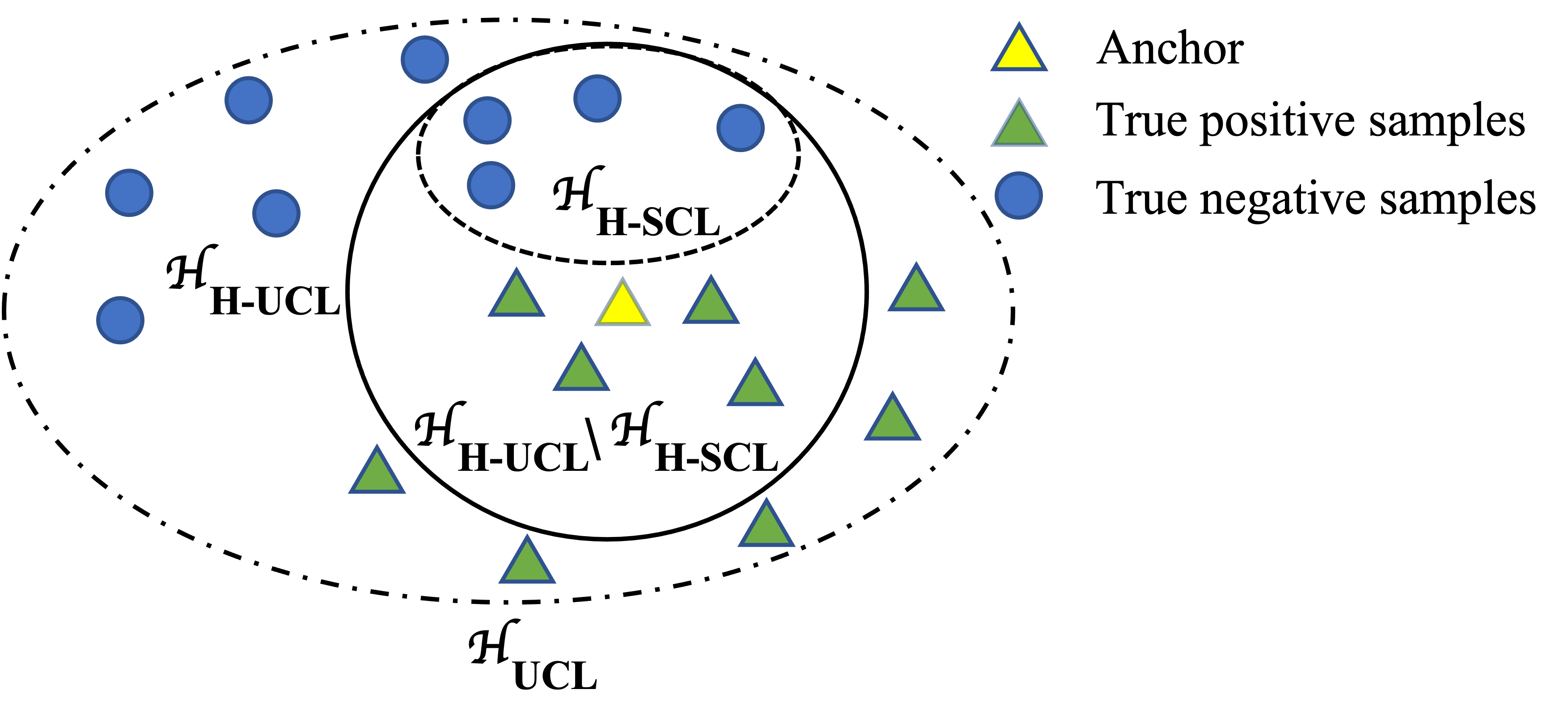
First, recall that $\mathcal{H}_{\textup{\tiny H-SCL}}$ denotes the set of hard negative samples under H-SCL settings, and $\mathcal{H}_{\textup{\tiny H-UCL}}$ denotes the set of hard negative samples under H-UCL settings. For given $(v,v^{+})$ and $f$, $\mathcal{H}_{\textup{\tiny H-SCL}}$ and $\mathcal{H}_{\textup{\tiny H-UCL}}$ both depend on threshold $\tau$. To enable the comparison, for given $(v,v^{+})$ and $f$, the same threshold $\tau$ is used under both H-SCL and H-UCL settings. Next, we begin with an assumption.

Assumption 1.

For any given $(v,v^{+})$, $f$, and a threshold $\tau$ which is used to construct both $\mathcal{H}_{\textup{\tiny H-SCL}}$ and $\mathcal{H}_{\textup{\tiny H-UCL}}$, let:

$$q_{\textup{\tiny H-UCL $\setminus$ H-SCL}}(v_{j}^{-})=\mathbb{E}_{c\sim\rho}\leavevmode\nobreak\ \mathcal{D}_{c}(v_{j}^{-}|\mathcal{H}_{\textup{\tiny H-UCL}}\setminus\mathcal{H}_{\textup{\tiny H-SCL}}),$$ (16)

where $\mathcal{D}_{c}(\cdot|\cdot)$ is defined in Eq. (2) and “$\setminus$" denotes the set subtraction operation, assume that:

$$\mathbb{E}_{\begin{subarray}{c}v_{j}^{-}\sim q_{\textup{\tiny H-UCL $\setminus$ H-SCL}}\end{subarray}}\big{[}e^{g(v,v_{j}^{-})}\big{|}v_{j}^{-}\in\mathcal{H}_{\textup{\tiny H-UCL}}\setminus\mathcal{H}_{\textup{\tiny H-SCL}}\big{]}$$ (17)

$$\geq \mathbb{E}_{\begin{subarray}{c}v_{j}^{-}\sim q_{\textup{\tiny H-SCL}}\end{subarray}}\big{[}e^{g(v,v_{j}^{-})}\big{|}v_{j}^{-}\in\mathcal{H}_{\textup{\tiny H-SCL}}\big{]}.$$

Note that from Eq. (14), $\mathcal{H}_{\textup{\tiny H-SCL}}\subset\mathcal{H}_{\textup{\tiny H-UCL}}$. Next, by definition, $\mathcal{H}_{\textup{\tiny H-SCL}}$ only contains the samples that have different labels with $v$. Because for given $v$ and $f$, we use the same threshold $\tau$ to construct both $\mathcal{H}_{\textup{\tiny H-UCL}}$ and $\mathcal{H}_{\textup{\tiny H-SCL}}$, thus, $\mathcal{H}_{\textup{\tiny H-UCL}}\setminus\mathcal{H}_{\textup{\tiny H-SCL}}$ must contain the samples having the same label with $v$. Fig. 3 illustrates the relationship between $\mathcal{H}_{\textup{\tiny H-UCL}}$, $\mathcal{H}_{\textup{\tiny H-SCL}}$, and $\mathcal{H}_{\textup{\tiny H-UCL}}\setminus\mathcal{H}_{\textup{\tiny H-SCL}}$. In other words, Assumption 1 assumes that the expected distance between the anchor $v$ to the samples having the same label (samples in $\mathcal{H}_{\textup{\tiny H-UCL}}\setminus\mathcal{H}_{\textup{\tiny H-SCL}}$) is smaller or at most equal to the expected distance between $v$ to the samples having different labels (samples in $\mathcal{H}_{\textup{\tiny H-SCL}}$). As previously discussed in Sec. 3, because normalization is used in contrastive learning, a smaller distance between two points corresponds to a larger value produced by the dot product, leading to the inequality in Assumption 1. In practice, the Assumption 1 is reasonable if the representation function $f$ is a good mapping, i.e., under mapping $f$, points having the same label are pulled close to each other while points having different labels are pushed far apart. In Sec. 6, we will numerically verify Assumption 1.

Figure 3: For a given $v$ (anchor, yellow triangle) and a threshold $\tau$, $\mathcal{H}_{\textup{\tiny H-UCL}}$ contains all the negative samples $v_{j}^{-}$ in the solid-line circle that satisfy the constraint $e^{g(v,v_{j}^{-})}\geq\tau$. $\mathcal{H}_{\textup{\tiny H-SCL}}$ is a subset of $\mathcal{H}_{\textup{\tiny H-UCL}}$ and only contains the true negative samples (blue circles) while $\mathcal{H}_{\textup{\tiny H-UCL}}\setminus\mathcal{H}_{\textup{\tiny H-SCL}}$ only contains the true positive samples (green triangles). Here, true positive samples mean the samples having the same label with the anchor while true negative samples mean the samples having different labels with the anchor.

Lemma 5.1.

Under Assumption 1, if $k\rightarrow+\infty$, then:

$$\mathcal{L}_{\textup{ \tiny H-SCL}}\,\leq\,\mathcal{L}_{\textup{ \tiny H-UCL}}.$$ (18)

Proof.

From the definitions of $\mathcal{L}_{\textup{ \tiny H-UCL}}$ and $\mathcal{L}_{\textup{ \tiny H-SCL}}$ in (11) and (15), for given $f$, $(v,v^{+})$ and its corresponding $\tau$, if $k\rightarrow+\infty$, we need to show that:

$$\mathbb{E}_{v,v^{+}\sim p}\,\mathbb{E}_{v_{1:k}^{-}\sim q_{\textup{\tiny H-SCL}}}\Big{[}\log\Big{(}e^{g(v,v^{+})}+\dfrac{1}{k}\sum_{j=1}^{k}e^{g(v,v_{j}^{-})}\Big{)}\Big{]}$$

$$\leq\mathbb{E}_{v,v^{+}\sim p}\,\mathbb{E}_{v_{1:k}^{-}\sim q_{\textup{\tiny H-UCL}}}\Big{[}\!\log\!\Big{(}e^{g(v,v^{+})}\!+\!\dfrac{1}{k}\!\sum_{j=1}^{k}e^{g(v,v_{j}^{-})}\!\Big{)}\!\Big{]}.$$

(19)

When $k\rightarrow+\infty$, Eq. (19) is equivalent to:

$$\mathbb{E}_{v,v^{+}\sim p}\Big{[}\log\Big{(}e^{g(v,v^{+})}+\mathbb{E}_{v_{j}^{-}\sim q_{\textup{\tiny H-SCL}}}[e^{g(v,v_{j}^{-})}]\Big{)}\Big{]}$$

$$\leq\mathbb{E}_{v,v^{+}\sim p}\Big{[}\log\Big{(}e^{g(v,v^{+})}+\mathbb{E}_{v_{j}^{-}\sim q_{\textup{\tiny H-UCL}}}[e^{g(v,v_{j}^{-})}]\Big{)}\Big{]}.$$

(20)

Since $\log(\cdot)$ is a monotonically increasing function and $e^{g(v,v^{+})}$ is shared between two sides of Eq. (20), we need to show that:

$$\mathbb{E}_{v_{j}^{-}\sim q_{\textup{\tiny H-UCL}}}\big{[}e^{g(v,v_{j}^{-})}\big{|}v_{j}^{-}\in\mathcal{H}_{\textup{\tiny H-UCL}}\big{]}$$

$$\geq\mathbb{E}_{v_{j}^{-}\sim q_{\textup{\tiny H-SCL}}}\big{[}e^{g(v,v_{j}^{-})}\big{|}v_{j}^{-}\in\mathcal{H}_{\textup{\tiny H-SCL}}\big{]}.$$ (21)

Indeed, from Assumption 1 and note that $\mathcal{H}_{\textup{\tiny H-SCL}}\subset\mathcal{H}_{\textup{\tiny H-UCL}}$, we have:

$$\mathbb{E}_{\begin{subarray}{c}v_{j}^{-}\sim q_{\textup{\tiny H-UCL}}\end{subarray}}\big{[}e^{g(v,v_{j}^{-})}\big{|}v_{j}^{-}\in\mathcal{H}_{\textup{\tiny H-UCL}}\big{]}$$ (22)

$$= \dfrac{P({\mathcal{H}_{\textup{\tiny H-SCL}}})}{P({\mathcal{H}_{\textup{\tiny H-UCL}}})}\mathbb{E}_{\begin{subarray}{c}v_{j}^{-}\sim q_{\textup{\tiny H-SCL}}\end{subarray}}\big{[}e^{g(v,v_{j}^{-})}\big{|}v_{j}^{-}\in\mathcal{H}_{\textup{\tiny H-SCL}}\big{]}$$

$$+ \dfrac{P(\mathcal{H}_{\textup{\tiny H-UCL}}\setminus\mathcal{H}_{\textup{\tiny H-SCL}})}{P({\mathcal{H}_{\textup{\tiny H-UCL}}})}$$

$$\times \mathbb{E}_{\begin{subarray}{c}v_{j}^{-}\sim q_{\textup{\tiny H-UCL $\setminus$ H-SCL}}\end{subarray}}\big{[}e^{g(v,v_{j}^{-})}\big{|}v_{j}^{-}\in\mathcal{H}_{\textup{\tiny H-UCL}}\setminus\mathcal{H}_{\textup{\tiny H-SCL}}\big{]}$$

$$\geq \dfrac{P({\mathcal{H}_{\textup{\tiny H-SCL}}})}{P({\mathcal{H}_{\textup{\tiny H-UCL}}})}\mathbb{E}_{\begin{subarray}{c}v_{j}^{-}\sim q_{\textup{\tiny H-SCL}}\end{subarray}}\big{[}e^{g(v,v_{j}^{-})}\big{|}v_{j}^{-}\in\mathcal{H}_{\textup{\tiny H-SCL}}\big{]}$$

$$+ \Big{(}1-\dfrac{P({\mathcal{H}_{\textup{\tiny H-SCL}}})}{P({\mathcal{H}_{\textup{\tiny H-UCL}}})}\Big{)}$$

$$\times \mathbb{E}_{\begin{subarray}{c}v_{j}^{-}\sim q_{\textup{\tiny H-SCL}}\end{subarray}}\big{[}e^{g(v,v_{j}^{-})}\big{|}v_{j}^{-}\in\mathcal{H}_{\textup{\tiny H-SCL}}\big{]}$$

$$= \mathbb{E}_{\begin{subarray}{c}v_{j}^{-}\sim q_{\textup{\tiny H-SCL}}\end{subarray}}\big{[}e^{g(v,v_{j}^{-})}\big{|}v_{j}^{-}\in\mathcal{H}_{\textup{\tiny H-SCL}}\big{]}$$ (23)

where $P(\mathcal{A})$ denotes the probability of set $\mathcal{A}$ and Eq. (22) due to Assumption 1.

Finally, Eq. (19) holds by combining Eq. (20), Eq. (5), and Eq. (23). The proof is complete. ∎

Lemma 5.1 showed that the loss function of H-UCL can be used as a proxy to optimize the loss function of H-SCL under some certain conditions. Because Lemma 5.1 requires $k\rightarrow+\infty$, a large value of $k$ is preferred in practice. This agrees with the numerical results in He et al. (2020); Wu et al. (2020); Zhuang et al. (2019); Iscen et al. (2019); Srinivas et al. (2020) where large values of $k$ lead to higher accuracies in downstream tasks.

Next, we show that the loss function of UCL ($\mathcal{L}_{\textup{ \tiny UCL}}$) is not an upper bound for the loss function of H-SCL ($\mathcal{L}_{\textup{ \tiny H-SCL}}$).

Lemma 5.2.

For any given $(v,v^{+})$ and $f$, if $k\rightarrow+\infty$, by selecting

$$\tau\geq\mathbb{E}_{v_{j}^{-}\sim q_{\textup{\tiny UCL}}}\big{[}e^{g(v,v_{j}^{-})}\big{|}v_{j}^{-}\in\mathcal{H}_{\textup{\tiny UCL}}\big{]}$$ (24)

then:

$$\mathcal{L}_{\textup{ \tiny UCL}}\,\leq\,\mathcal{L}_{\textup{ \tiny H-SCL}}.$$ (25)

Proof.

From the definitions of $\mathcal{L}_{\textup{ \tiny UCL}}$ and $\mathcal{L}_{\textup{ \tiny H-SCL}}$ in (10) and (15), for given $f$, $(v,v^{+})$ and its corresponding $\tau$, if $k\rightarrow+\infty$, we need to show that:

$$\mathbb{E}_{v,v^{+}\sim p}\,\mathbb{E}_{v_{1:k}^{-}\sim q_{\textup{\tiny UCL}}}\Big{[}\log\Big{(}e^{g(v,v^{+})}+\dfrac{1}{k}\sum_{j=1}^{k}e^{g(v,v_{j}^{-})}\Big{)}\Big{]}$$

$$\leq\mathbb{E}_{v,v^{+}\sim p}\,\mathbb{E}_{v_{1:k}^{-}\sim q_{\textup{\tiny H-SCL}}}\Big{[}\!\log\!\Big{(}e^{g(v,v^{+})}\!+\!\dfrac{1}{k}\!\sum_{j=1}^{k}e^{g(v,v_{j}^{-})}\!\Big{)}\!\Big{]}.$$

Similar to the proof of Lemma 5.1, by taking the limitations when $k\rightarrow+\infty$ as in Eq. (20), we need to show that:

$$\mathbb{E}_{v_{j}^{-}\sim q_{\textup{\tiny H-SCL}}}\big{[}e^{g(v,v_{j}^{-})}\big{|}v_{j}^{-}\in\mathcal{H}_{\textup{\tiny H-SCL}}\big{]}$$

$$\geq\mathbb{E}_{v_{j}^{-}\sim q_{\textup{\tiny UCL}}}\big{[}e^{g(v,v_{j}^{-})}\big{|}v_{j}^{-}\in\mathcal{H}_{\textup{\tiny UCL}}\big{]}.$$ (26)

Note that $\mathcal{H}_{\textup{\tiny H-SCL}}$ only contains the samples $v_{j}^{-}$ such that $e^{g(v,v_{j}^{-})}\geq\tau$, the left-hand-side of Eq. (5) is greater than $\tau$. Thus, by selecting $\tau$ that satisfies Eq. (24), the right-hand-side of Eq. (5) is less than $\tau$, thus, Eq. (5) holds. The proof is complete. ∎

Note that Lemma 5.2 is only a simple counter-example and, in general, there is no clear relationship between $\mathcal{L}_{\textup{ \tiny UCL}}$ and $\mathcal{L}_{\textup{ \tiny H-SCL}}$ as we pointed out in Sec. 6.4.

6 Numerical results

In this section, we demonstrate the efficiency of H-SCL over other competing methods on three image datasets. In addition, we also empirically verify Assumption 1 which supports our claim that $\mathcal{L}_{\textup{\tiny H-SCL}}\leq\mathcal{L}_{\textup{\tiny H-UCL}}$.

6.1 Datasets

We evaluated UCL, H-UCL, SCL, and H-SCL on three datasets: STL10 Coates et al. (2011), CIFAR10, and CIFAR100 Krizhevsky et al. (2009) for visual representation learning which contain images with 10, 10, and 100 classes, respectively.

6.2 Experiment setup

We adopt the simulation set-up and practical implementation from Khosla et al. (2020).

In practice, for selecting the hard negative samples, we utilize the method proposed in Robinson et al. (2021). Specifically, Robinson et al. use a hyper-parameter $\beta>0$ to practically control the hardness of sampling strategies by assigning a higher probability to the sample that is closer to the anchor:

$$q_{\textup{\tiny H-SCL}}(v_{j}^{-})\,\propto\,e^{\beta\,g(v,v_{j}^{-})}q_{\textup{\tiny SCL}}(v_{j}^{-}),$$ (27)

$$q_{\textup{\tiny H-UCL}}(v_{j}^{-})\,\propto\,e^{\beta\,g(v,v_{j}^{-})}q_{\textup{\tiny UCL}}(v_{j}^{-}),$$ (28)

where $\propto$ means that the distributions will be normalized after multiplying with its corresponding weight $e^{\beta\,g(v,v_{j}^{-})}$ that depends on the distance between the negative sample and its anchor. Note that for most theoretical papers, for the simplicity of analysis, a “hard" threshold $\tau$ is used to control the hardness of sampling. However, in practice, $\beta$ is used as a “soft" threshold to control the hardness by assigning a high selection probability to the sample that is close to the anchor.

The practical loss function we used to learn the representation function $f$ is:

$$\mathbb{E}_{v,v^{+}\sim p}\left[\log\left(1+\frac{o}{e^{g(v,v^{+})}}\,\mathbb{E}_{v_{j}^{-}\sim q}\big{[}e^{g(v,v_{j}^{-})}\big{]}\right)\right]$$ (29)

where $o$ is scalar that balances the contributions between positive and negative samples in the loss function, the negative distribution $q$ is selected from $\{q_{\textup{\tiny UCL}},q_{\textup{\tiny SCL}},q_{\textup{\tiny H-UCL}},q_{\textup{\tiny H-SCL}}\}$ corresponding to UCL, SCL, H-UCL, and H-SCL settings, respectively. For a given negative distribution, the expectation $\mathbb{E}_{v_{j}^{-}\sim q}\big{[}e^{g(v,v_{j}^{-})}\big{]}$ in Eq. (29) is empirically approximated over a batch of training samples.

We use ResNet-50 (He et al., 2015) with a representation dimension of 2048 and a projection head with a dimension of 128 to learn the representation function. After fixing the representation function generated by the trained ResNet-50, we train a linear classifier to output the final classification accuracies. Our code is released at this link.

6.3 Training procedure

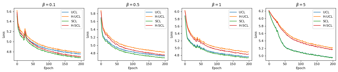
All models are trained for 200 epochs with a batch size of 512. We use the Adam optimizer with the learning rate of 0.001 and weight decay of 10^-6. There is only one hyper-parameter need to be tuned which is $\beta$. Here, we perform a grid search of $\beta$ over the set of $\{0.1,0.5,1,2,5\}$ and set $o$ (in Eq. (29)) equal to the batch size. NVIDIA A100 32 GB GPU is used for computations and it takes about 10 hours to train one model (200 epochs) for each dataset. Since labeled STL10 is a small dataset, we repeat our experiment five times on this dataset and report the average accuracy together with its standard deviation.

Dataset	UCL	H-UCL	SCL	H-SCL (our)
STL10	64.36 $\pm$ 0.92	67.82 $\pm$ 1.41	68.28 $\pm$ 0.92	72.52 $\pm$ 1.94
CIFAR10	89.16	90.35	93.46	93.98
CIFAR100	64.02	67.77	71.68	75.11

Table 1: The best accuracies of tested methods on three datasets (in %).

Figure 4: Values of different loss functions $\mathcal{L}_{\textup{\tiny UCL}}$, $\mathcal{L}_{\textup{\tiny H-UCL}}$, $\mathcal{L}_{\textup{\tiny SCL}}$, and $\mathcal{L}_{\textup{\tiny H-SCL}}$ with different degree of hardness $\beta=0.1,0.5,1,5$ on STL10 dataset. We train the representation function $f$ with $\mathcal{L}_{\textup{\tiny H-UCL}}$, then fix $f$ to calculate $\mathcal{L}_{\textup{\tiny H-UCL}}$, $\mathcal{L}_{\textup{\tiny SCL}}$, and $\mathcal{L}_{\textup{\tiny H-SCL}}$ separately.

6.4 Results

Tables 1 compares the best accuracies of UCL, H-UCL, SCL, and H-SCL attained on three image datasets. As seen, H-SCL consistently outperforms other methods with the margins of at least 3% on CIFAR100 and 4% on STL10, respectively. However, H-SCL is just slightly better than SCL on CIFAR10. Due to the limited space, we only provide the accuracies of tested methods corresponding to the number of epochs on CIFAR100 as shown in Fig. 1. As seen, H-SCL only requires less than 50 epochs to achieve the same accuracy as SCL at 200 epochs.

Next, to verify Assumption 1, we compute the average values of the left-hand-side and the right-hand-side in Eq. (17) on STL10 dataset as an example. Our results indicate that the average value of the left-hand-side of (17) is 1.44 which is quite larger than the average value of the right-hand-side of (17) which is 0.99.

Finally, Fig. 4 practically verifies the correctness of the results in Lemma 5.1 and Lemma 5.2. Specifically, depending on the values of $\beta$, $\mathcal{L}_{\textup{\tiny H-SCL}}$ (red curves) can be upper bounded (see $\beta=0.1$) or lower bounded (see $\beta=0.5$ and $\beta=1$) by $\mathcal{L}_{\textup{\tiny UCL}}$ (blue curves) while $\mathcal{L}_{\textup{\tiny H-SCL}}$ (red curves) is always upper bounded by $\mathcal{L}_{\textup{\tiny H-UCL}}$ (orange curves).

7 Conclusion and discussion

In this paper, we introduced a new framework called hard-negative supervised contrastive learning which utilizes both the label information and the hard-negative sampling strategies to improve the learning performance. We demonstrated the efficiency of hard-negative supervised contrastive learning against other contrastive learning approaches over several real datasets. Interestingly, we pointed out that the loss function of hard-negative supervised contrastive learning can be bounded by the loss function of hard-negative unsupervised contrastive learning which suggests a way to justify why the hard-negative unsupervised contrastive learning outperforms the unsupervised contrastive learning in practice.

Our future work will focus on extending the current setting which uses only one positive sample to a general setting that can handle multiple positive samples. In addition, motivated by the success of hard-negative sampling strategies, investigating the usefulness of hard-positive sampling strategies, i.e., selecting the positive samples which are hard to discern with negative samples will be considered as another direction of our future work.

References

- Bjorck et al. (2021) J. Bjorck, B. H. Rappazzo, Q. Shi, C. Brown-Lima, J. Dean, A. Fuller, and C. Gomes. Accelerating ecological sciences from above: Spatial contrastive learning for remote sensing. In Proceedings of the AAAI Conference on Artificial Intelligence, volume 35, pages 14711–14720, 2021.
- Chen et al. (2022) J. Chen, R. Zhang, Y. Mao, and J. Xu. Contrastnet: A contrastive learning framework for few-shot text classification. In Proceedings of the AAAI Conference on Artificial Intelligence, volume 36, pages 10492–10500, 2022.
- Chen et al. (2020) T. Chen, S. Kornblith, M. Norouzi, and G. Hinton. A simple framework for contrastive learning of visual representations. In International conference on machine learning, pages 1597–1607. PMLR, 2020.
- Chopra et al. (2005) S. Chopra, R. Hadsell, and Y. LeCun. Learning a similarity metric discriminatively, with application to face verification. In 2005 IEEE Computer Society Conference on Computer Vision and Pattern Recognition (CVPR’05), volume 1, pages 539–546. IEEE, 2005.
- Coates et al. (2011) A. Coates, A. Ng, and H. Lee. An analysis of single-layer networks in unsupervised feature learning. In Proceedings of the fourteenth international conference on artificial intelligence and statistics, pages 215–223. JMLR Workshop and Conference Proceedings, 2011.
- Fang et al. (2022) Y. Fang, Q. Zhang, H. Yang, X. Zhuang, S. Deng, W. Zhang, M. Qin, Z. Chen, X. Fan, and H. Chen. Molecular contrastive learning with chemical element knowledge graph. In Proceedings of the AAAI Conference on Artificial Intelligence, volume 36, pages 3968–3976, 2022.
- Hadsell et al. (2006) R. Hadsell, S. Chopra, and Y. LeCun. Dimensionality reduction by learning an invariant mapping. In 2006 IEEE Computer Society Conference on Computer Vision and Pattern Recognition (CVPR’06), volume 2, pages 1735–1742. IEEE, 2006.
- He et al. (2015) K. He, X. Zhang, S. Ren, and J. Sun. Deep residual learning for image recognition. arXiv preprint arXiv:1512.03385, 2015.
- He et al. (2020) K. He, H. Fan, Y. Wu, S. Xie, and R. Girshick. Momentum contrast for unsupervised visual representation learning. In Proceedings of the IEEE/CVF conference on computer vision and pattern recognition, pages 9729–9738, 2020.
- Henaff (2020) O. Henaff. Data-efficient image recognition with contrastive predictive coding. In International conference on machine learning, pages 4182–4192. PMLR, 2020.
- Iscen et al. (2019) A. Iscen, G. Tolias, Y. Avrithis, and O. Chum. Label propagation for deep semi-supervised learning. In Proceedings of the IEEE/CVF Conference on Computer Vision and Pattern Recognition, pages 5070–5079, 2019.
- Kalantidis et al. (2020) Y. Kalantidis, M. B. Sariyildiz, N. Pion, P. Weinzaepfel, and D. Larlus. Hard negative mixing for contrastive learning. Advances in Neural Information Processing Systems, 33:21798–21809, 2020.
- Khosla et al. (2020) P. Khosla, P. Teterwak, C. Wang, A. Sarna, Y. Tian, P. Isola, A. Maschinot, C. Liu, and D. Krishnan. Supervised contrastive learning. Advances in Neural Information Processing Systems, 33:18661–18673, 2020.
- Kim and Song (2021) D. H. Kim and B. C. Song. Contrastive adversarial learning for person independent facial emotion recognition. In AAAI, pages 5948–5956, 2021.
- Krizhevsky et al. (2009) A. Krizhevsky, G. Hinton, et al. Learning multiple layers of features from tiny images. 2009.
- Li et al. (2021) Y. Li, P. Hu, Z. Liu, D. Peng, J. T. Zhou, and X. Peng. Contrastive clustering. In Proceedings of the AAAI Conference on Artificial Intelligence, volume 35, pages 8547–8555, 2021.
- Liang et al. (2022) D. Liang, L. Li, M. Wei, S. Yang, L. Zhang, W. Yang, Y. Du, and H. Zhou. Semantically contrastive learning for low-light image enhancement. In Proceedings of the AAAI Conference on Artificial Intelligence, volume 36, pages 1555–1563, 2022.
- Liu et al. (2021) C. Liu, Y. Fu, C. Xu, S. Yang, J. Li, C. Wang, and L. Zhang. Learning a few-shot embedding model with contrastive learning. In Proceedings of the AAAI Conference on Artificial Intelligence, volume 35, pages 8635–8643, 2021.
- Liu et al. (2022) H. Liu, B. Wang, Z. Bao, M. Xue, S. Kang, D. Jiang, Y. Liu, and B. Ren. Perceiving stroke-semantic context: Hierarchical contrastive learning for robust scene text recognition. AAAI, 2022.
- Mo et al. (2022) Y. Mo, L. Peng, J. Xu, X. Shi, and X. Zhu. Simple unsupervised graph representation learning. AAAI, 2022.
- Mohsenvand et al. (2020) M. N. Mohsenvand, M. R. Izadi, and P. Maes. Contrastive representation learning for electroencephalogram classification. In Machine Learning for Health, pages 238–253. PMLR, 2020.
- Nonnenmacher et al. (2022) M. T. Nonnenmacher, L. Oldenburg, I. Steinwart, and D. Reeb. Utilizing expert features for contrastive learning of time-series representations. In International Conference on Machine Learning, pages 16969–16989. PMLR, 2022.
- Oord et al. (2018) A. v. d. Oord, Y. Li, and O. Vinyals. Representation learning with contrastive predictive coding. arXiv preprint arXiv:1807.03748, 2018.
- Pan et al. (2022) L. Pan, C.-W. Hang, A. Sil, and S. Potdar. Improved text classification via contrastive adversarial training. In Proceedings of the AAAI Conference on Artificial Intelligence, volume 36, pages 11130–11138, 2022.
- Pang et al. (2022) B. Pang, Y. Li, Y. Zhang, G. Peng, J. Tang, K. Zha, J. Li, and C. Lu. Unsupervised representation for semantic segmentation by implicit cycle-attention contrastive learning. AAAI, 2022.
- Rethmeier and Augenstein (2021) N. Rethmeier and I. Augenstein. A primer on contrastive pretraining in language processing: Methods, lessons learned and perspectives. arXiv preprint arXiv:2102.12982, 2021.
- Robinson et al. (2020) J. Robinson, C.-Y. Chuang, S. Sra, and S. Jegelka. Contrastive learning with hard negative samples. arXiv preprint arXiv:2010.04592, 2020.
- Robinson et al. (2021) J. D. Robinson, C.-Y. Chuang, S. Sra, and S. Jegelka. Contrastive learning with hard negative samples. In International Conference on Learning Representations, 2021. URL https://openreview.net/forum?id=CR1XOQ0UTh-.
- Shi et al. (2019) J. Shi, C. Liang, L. Hou, J. Li, Z. Liu, and H. Zhang. Deepchannel: Salience estimation by contrastive learning for extractive document summarization. In Proceedings of the AAAI Conference on Artificial Intelligence, volume 33, pages 6999–7006, 2019.
- Shi et al. (2021) T. Shi, L. Li, P. Wang, and C. K. Reddy. A simple and effective self-supervised contrastive learning framework for aspect detection. In Proceedings of the AAAI Conference on Artificial Intelligence, volume 35, pages 13815–13824, 2021.
- Srinivas et al. (2020) A. Srinivas, M. Laskin, and P. Abbeel. Curl: Contrastive unsupervised representations for reinforcement learning. arXiv preprint arXiv:2004.04136, 2020.
- Sun et al. (2022) K. Sun, T. Yao, S. Chen, S. Ding, J. Li, and R. Ji. Dual contrastive learning for general face forgery detection. In Proceedings of the AAAI Conference on Artificial Intelligence, volume 36, pages 2316–2324, 2022.
- Tabassum et al. (2022) A. Tabassum, M. Wahed, H. Eldardiry, and I. Lourentzou. Hard negative sampling strategies for contrastive representation learning. arXiv preprint arXiv:2206.01197, 2022.
- Tian et al. (2020a) Y. Tian, D. Krishnan, and P. Isola. Contrastive multiview coding. In European conference on computer vision, pages 776–794. Springer, 2020a.
- Tian et al. (2020b) Y. Tian, C. Sun, B. Poole, D. Krishnan, C. Schmid, and P. Isola. What makes for good views for contrastive learning? Advances in Neural Information Processing Systems, 33:6827–6839, 2020b.
- Wan et al. (2021) S. Wan, S. Pan, J. Yang, and C. Gong. Contrastive and generative graph convolutional networks for graph-based semi-supervised learning. In Proceedings of the AAAI Conference on Artificial Intelligence, volume 35, pages 10049–10057, 2021.
- Wang et al. (2021) J. Wang, Y. Gao, K. Li, J. Hu, X. Jiang, X. Guo, R. Ji, and X. Sun. Enhancing unsupervised video representation learning by decoupling the scene and the motion. In Proceedings of the AAAI Conference on Artificial Intelligence, volume 35, pages 10129–10137, 2021.
- Wu et al. (2017) C.-Y. Wu, R. Manmatha, A. J. Smola, and P. Krahenbuhl. Sampling matters in deep embedding learning. In Proceedings of the IEEE International Conference on Computer Vision, pages 2840–2848, 2017.
- Wu et al. (2020) M. Wu, M. Mosse, C. Zhuang, D. Yamins, and N. Goodman. Conditional negative sampling for contrastive learning of visual representations. arXiv preprint arXiv:2010.02037, 2020.
- Wu et al. (2018) Z. Wu, A. A. Efros, and S. X. Yu. Improving generalization via scalable neighborhood component analysis. In Proceedings of the European Conference on Computer Vision (ECCV), pages 685–701, 2018.
- Yang et al. (2022) C. Yang, Z. An, L. Cai, and Y. Xu. Mutual contrastive learning for visual representation learning. In Proceedings of the AAAI Conference on Artificial Intelligence, volume 36, pages 3045–3053, 2022.
- Yao et al. (2022) L. Yao, W. Wang, and Q. Jin. Image difference captioning with pre-training and contrastive learning. arXiv preprint arXiv:2202.04298, 1(4), 2022.
- Ye et al. (2021) H. Ye, N. Zhang, S. Deng, M. Chen, C. Tan, F. Huang, and H. Chen. Contrastive triple extraction with generative transformer. In Proceedings of the AAAI conference on artificial intelligence, volume 35, pages 14257–14265, 2021.
- Yin et al. (2022) Y. Yin, Q. Wang, S. Huang, H. Xiong, and X. Zhang. Autogcl: Automated graph contrastive learning via learnable view generators. In Proceedings of the AAAI Conference on Artificial Intelligence, volume 36, pages 8892–8900, 2022.
- You et al. (2020) Y. You, T. Chen, Y. Sui, T. Chen, Z. Wang, and Y. Shen. Graph contrastive learning with augmentations. Advances in Neural Information Processing Systems, 33:5812–5823, 2020.
- Yu et al. (2022) L. Yu, S. Pei, L. Ding, J. Zhou, L. Li, C. Zhang, and X. Zhang. Sail: Self-augmented graph contrastive learning. In Proceedings of the AAAI Conference on Artificial Intelligence, volume 36, pages 8927–8935, 2022.
- Yuan et al. (2017) Y. Yuan, K. Yang, and C. Zhang. Hard-aware deeply cascaded embedding. In Proceedings of the IEEE international conference on computer vision, pages 814–823, 2017.
- Zhai et al. (2019) X. Zhai, A. Oliver, A. Kolesnikov, and L. Beyer. S4l: Self-supervised semi-supervised learning. In Proceedings of the IEEE/CVF International Conference on Computer Vision, pages 1476–1485, 2019.
- Zhang et al. (2022a) X. Zhang, B. Zhu, X. Yao, Q. Sun, R. Li, and B. Yu. Context-based contrastive learning for scene text recognition. In Proceedings of the AAAI Conference on Artificial Intelligence. AAAI, 2022a.
- Zhang et al. (2022b) Y. Zhang, L.-M. Po, X. Xu, M. Liu, Y. Wang, W. Ou, Y. Zhao, and W.-Y. Yu. Contrastive spatio-temporal pretext learning for self-supervised video representation. In Proceedings of the AAAI Conference on Artificial Intelligence, volume 36, pages 3380–3389, 2022b.
- Zhuang et al. (2019) C. Zhuang, A. L. Zhai, and D. Yamins. Local aggregation for unsupervised learning of visual embeddings. In Proceedings of the IEEE/CVF International Conference on Computer Vision, pages 6002–6012, 2019.