Automatic Dynamic Relevance Determination
for Gaussian process regression
with high-dimensional functional inputs

Abstract

In the context of Gaussian process regression with functional inputs, it is common to treat the input as a vector. The parameter space becomes prohibitively complex as the number of functional points increases, effectively becoming a hindrance for automatic relevance determination in high-dimensional problems. Generalizing a framework for time-varying inputs, we introduce the asymmetric Laplace functional weight (ALF): a flexible, parametric function that drives predictive relevance over the index space. Automatic dynamic relevance determination (ADRD) is achieved with three unknowns per input variable and enforces smoothness over the index space. Additionally, we discuss a screening technique to assess under complete absence of prior and model information whether ADRD is reasonably consistent with the data. Such tool may serve for exploratory analyses and model diagnostics. ADRD is applied to remote sensing data and predictions are generated in response to atmospheric functional inputs. Fully Bayesian estimation is carried out to identify relevant regions of the functional input space. Validation is performed to benchmark against traditional vector-input model specifications. We find that ADRD outperforms models with input dimension reduction via functional principal component analysis. Furthermore, the predictive power is comparable to high-dimensional models, in terms of both mean prediction and uncertainty, with 10 times fewer tuning parameters. Enforcing smoothness on the predictive relevance profile rules out erratic patterns associated with vector-input models.

Keywords: Functional Input, Gaussian process, surrogate, metamodeling, computer experiments

1 Introduction

The study of uncertainty in complex physical systems commonly relies on the evaluation of computationally expensive computer models. Many science and engineering computer models approximate systems that include functional inputs, i.e., input quantities varying over a continuum typically modeled as function of some index. Dynamical systems are a widely popular sub-group of this family whose main characteristic is that the input, and possibly the output, is a function of time. In other settings, the index space could represent space or wavelengths.

Gaussian processes are a common choice among the many available statistical and machine learning models for computer model emulation, with early work such as sacks1989; sacks1989a; currin1991; ohagan1992; koehler1996; jones1998; kennedy2001. A modern, general treatment can be found in santner2018; gramacy2020. However, the literature mainly emphasizes the emulation of dynamical systems via Gaussian processes with scalar, vector scalar-summary, or possibly pre-processed vector inputs in relation to either a scalar output or a pre-processed structured output modeled as separable vector (campbell2006; bayarri2007a; higdon2008).

A simple modeling strategy is to consider the functional input not as functional, but an ensemble of possibly many scalar values and a specific correlation structure (iooss2009). Although straightforward, discretization leads to a potentially unlimited number of feature variables used to predict a finite number of scalar outputs, thus increasing model training difficulty and the risk of overfitting. Functional input pre-processing often involves the application of techniques for scaling, registration, warping, decorrelation, dimensionality reduction, and regularization. Frequently used ones are a-priori basis expansion, e.g., splines (betancourt2020; betancourt2020a), principal component analysis (nanty2016), functional principal component analysis (wang2017; wang2019), among other basis functions (tan2019; li2021). Such decompositions introduce undesirable side effects such as the laborious interpretation of non-physical variables, and the lack of direct use of the information contained in the input structure, e.g., the notions of order and closeness incorporated in the index space. These also struggle with the modeling and computational challenges associated with high-dimensional input vectors, principally a large number of unknowns and the risk of overfitting.

Whatever the approach, the complexity of present applications routinely warrants the use of regularization. Automatic relevance determination priors (neal1996) are prevalent in the world of Gaussian processes. Each input dimension, be a measurement from a functional profile or a basis coefficient, is given a different length-scale parameter that allows the latent function to vary at different speeds with respect to different inputs. This introduces multiple regularization as the marginal likelihood would favor solutions with large length-scales for those inputs along which the latent function is flat, a mechanism for Bayesian Occam’s razor put in place to prevent significant overfitting by pruning high-dimensional inputs toward sparse representations (mackay1996; wipf2007). In this context, relevance is defined as the inverse of the length-scale even though this quantity is also affected by other intrinsic characteristics of the data such as the output responding linearly or non-linearly to changes in the input variable (piironen2016). These length-scale parameters are sometimes known as correlation lengths (santner2018) or ranges (cressie1993), and their inverse as roughness (kennedy2001).

Relatively less work has been done to incorporate the input functional form into Gaussian process regression models, and the capabilities for automatic relevance determination in the developed methods are rather limited. Time-indexed input-output pairs for dynamical systems were discussed by morris2012, who proposed a half-normal weight function for time-indexed inputs where physical knowledge suggests a reversion to a neutral state or a reaction slowdown relative to some fixed time point. In this work, a point Bayesian estimate was produced for a computer experiment with five runs and a profile with 13 time steps. Later on, muehlenstaedt2017 presented two approaches for the $L^{2}$ norm for functional inputs via projection-based methodologies coupled with weights assigned to the basis functions. Such weights remain constant over the index space and originate in the discretization of the linear and beta distributions. kuttubekova2019 built a parametric weight via trigonometric basis functions of the functional index and predicted soil loss from daily precipitation and hill slope profiles with a one-harmonic Fourier expansion. Alternatively, chen2021 introduced kriging for functional inputs with functional weights in the spectral domain associating relevance quantities to each functional input frequency component rather than to the input measurements themselves.

With the ultimate goal of pushing the emulation of computer models with functional inputs closer to a hands-off process, we expand on these ideas and introduce a new functional weight parametric form for automatic dynamic relevance determination (ADRD). The asymmetric Laplace functional weight (ALF) learns from the data how the input predictive relevance varies across the input index space. Building off the notion that a predictive model may assign different weights across this index space, we set up a parametric weight function to enforce smoothness on relevance over the index space and allow the model to learn that some index subspaces are more relevant than others.

We describe the ALF methodology in Section 2, including procedures for fully-Bayesian estimation of the model parameters, model validation, and dynamic relevance screening in Sections 2.1, 2.2 and 2.3. In Section 3, we introduce a case study concerning the emulation of a computer model with functional inputs. We compare the posterior estimates for the automatic relevance determination parameters and out-of-sample predictive power across several plausible models and sets of input variables. Finally, we present in LABEL:sec:discussion potential improvements on our current work and delineate our future line of work.

2 Methods

Consider an experiment with a functional input $X(t)\in\mathcal{X}$ indexed by a continuous index $t\in\mathcal{T}$ and a scalar output $y\in\mathcal{Y}$. We model the unknown input-output relationship $f:\mathcal{X}\to\mathcal{Y}$ via a Gaussian process with mean function $m_{y}:\mathcal{X}\to\mathcal{Y}$ and a positive definite covariance function $s_{f}:\mathcal{X}^{2}\to{\mathbb{R}}^{+}$. Consider the squared exponential covariance function with homogeneous independent noise $s_{f}(X_{i},X_{j})=\sigma_{f}^{2}\ \exp\left\{-0.5\ d(X_{i},X_{j})\right\}$, $s_{y}(X_{i},X_{j})=s_{f}(X_{i},X_{j})+I_{i,j}\ \sigma_{\varepsilon}^{2},$ where $\sigma_{f}^{2}\in{\mathbb{R}}^{+}$ is the output signal variance, $\sigma_{\varepsilon}^{2}\in{\mathbb{R}}^{+}$ is the output noise variance, $I_{i,j}$ is an indicator function for $i=j$, and $i,j=1,\dots,N\in\mathbb{N}$ index the functional profiles. The function $d:\mathcal{X}^{2}\to{\mathbb{R}}^{+}$ quantifies the distance in any functional input pair. If the notion of a functional input is completely simplified to a $K-$dimensional vector input coupled with an automatic relevance determination (ARD) hierarchical prior for separable length-scale parameters, we have $d_{\textsc{ARD}}(X_{i},X_{j})=\sum_{k=1}^{K}{(x_{i,k}-x_{j,k})}^{2}/\sigma_{x_{k}}^{2}$ for $\sigma_{x_{k}}^{2}>0\ \forall\ k=1,\dots,K\in\mathbb{N}$. Alternatively, when the functional input is pre-processed via functional principal component analysis (ramsay2005), then $d_{\textsc{PC}}(X_{i},X_{j})=\sum_{{\tilde{k}}=1}^{{\tilde{K}}}{{({\tilde{x}}_{i,{\tilde{k}}}-{\tilde{x}}_{j,{\tilde{k}}})}^{2}}/\sigma^{2}_{{\tilde{x}}_{{\tilde{k}}}}$ for $\sigma_{{\tilde{x}}_{\tilde{k}}}^{2}>0\ \forall\ {\tilde{k}}=1,\dots,{\tilde{K}}\leq K$, where ${\tilde{x}}_{i,{\tilde{k}}}$ is the ${\tilde{k}}$-th score for the $i$-th profile and ${\tilde{K}}$ is the total number of principal components retained in the model.

Recognizing that the profile measurements $\mathbf{x}_{i}={\left\{x_{i,k}\right\}}_{k}$ are a finite representation of an infinite-dimensional function, we can quantify the distance between any two profile inputs via the weighted functional norm, i.e.,

$$d_{\omega}(X_{i},X_{j})=\phi^{-2}\int_{\mathcal{T}}\omega(t){\left(X_{i}(t)-X_{j}(t)\right)}^{2}\,\mathrm{d}t$$ (1)

where $\phi>0$ and $\omega:\mathcal{T}\to{\mathbb{R}}^{+}$ is a weight function driving the predictive relevance of the input on the output over the index space. A constraint is needed for $\omega(t)$ and $\phi$ to be identifiable, e.g., $\omega(t)=1$ for some $t\in\mathcal{T}$ or $\int_{\mathcal{T}}\,\omega(t)\,\mathrm{d}t=1$. The functional form of $\omega(t)$ is a modeling decision that opens up the possibility for domain-specific knowledge about the physical system; in truly complex settings, its specification might require a fully data-driven approach.

In practice, even if subsystems are well understood and documented, computer models consolidate a large number of interrelationships that may hinder prior relevance elicitation. In an effort to provide the weight function with enough flexibility for a more data-driven approach, we introduce the asymmetric Laplace functional weight (ALF),

$$\omega(t) =\text{exp}\left(-(t-\tau)\lambda\kappa^{s}s\right)=\begin{cases}\text{exp}\left(-\lambda_{1}\ \lvert t-\tau\rvert\right)&\text{for }t\leq\tau\\ \text{exp}\left(-\lambda_{2}\ \lvert t-\tau\rvert\right)&\text{for }t>\tau\\ \end{cases}$$ (2)

where we assume $\mathcal{T}=[0,1]$ without loss of generality, $s=\text{sign}(t-\tau)\in\{-1,1\}$, $\lambda>0$ is the rate, $\tau\in\mathcal{T}$ is the location, and $\kappa>0$ is the asymmetry coefficient. An alternative parametrization has $\lambda_{1}=\lambda\kappa^{-1}$ and $\lambda_{2}=\lambda\kappa$ for the left and right exponential decay rates around $\tau$. Figure 1 shows that ALF encompasses a wide family of functions such as the exponential decay ($\kappa=1,\tau=0$), exponential growth ($\kappa=1,\tau=1$), symmetric exponential with predictive relevance peak at $\tau$ ($\kappa=1$), near-zero weight before or after the location $\tau$ ($\lambda_{1}\to\infty$ or $\lambda_{2}\to\infty$), and constant weight before and after the location $\tau$ ($\lambda_{1}\to 0$ or $\lambda_{2}\to 0$).

This parametric function provides enough degrees of freedom for a rather wide range of unimodal patterns in predictive relevance with at most three parameters, attempting to find a balance in learnability and parameter space complexity compared to an ARD model with a typically large number of tuning unknowns. ALF offers a method to grow the resolution of the input profiles without compromising the parameter space complexity, effectively circumventing pre-processing decisions for input dimension reduction. Equally appealing, it enforces smoothness on predictive relevance over the index space ruling out erratic patterns for relevance in the fully-free ARD learnable space, e.g., $X(t_{k_{1}})$, $X(t_{k_{2}})$ and $X(t_{k_{3}})$ having disparate weights despite $t_{k_{1}}<t_{k_{2}}<t_{k_{3}}$ being close on the index space for the scale of the physical problem at hand. Besides making high-dimensional inputs more manageable, in situations where there is at least subsidiary interest in interpretable predictive modeling, ALF offers some insight in the input-output relationship by establishing an explicit link between the functional input index space and the output correlation. Such insight enters the predictive modeling feedback loop and may also foster the understanding of the underlying physical model. Overall, ALF attempts to produce a simplified representation that addresses interpretation, smoothness differentiation, and parsimony in relevance determination.

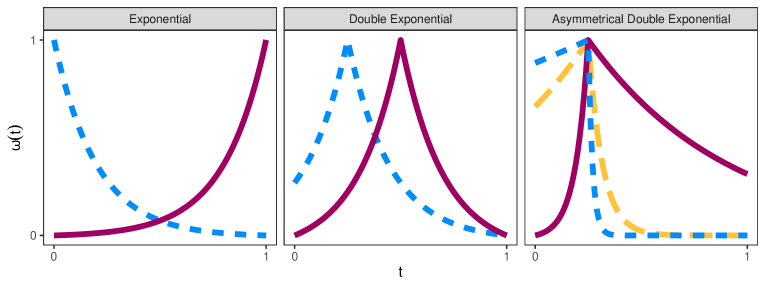
Figure 1: Some selected ALF configurations. Colors do not indicate grouping across facets.

2.1 Estimation

Consider the functional-input Gaussian process models (fiGP) with $d_{\omega}(\cdot)$ and the following configurations: $\kappa=1$ and $\tau=0$ decreasing exponential (fiGP-Edn), $\kappa=1$ symmetric double exponential (fiGP-SDE), and asymmetric double exponential with all three parameters free (fiGP-ADE). We use the umbrella term ALF to refer to these three models altogether since these are all parametrizations of Equation 2. We denote the parameter vector by $\bm{\theta}=(\bm{\theta}_{d},\sigma_{f}^{2},\sigma_{\varepsilon}^{2})$, where $\bm{\theta}_{d}$ encompasses the unknowns for a specific choice of $d(X_{i},X_{j})$, e.g., $\bm{\theta}_{d}=(\phi,\lambda,\kappa,\tau)$ for Equations 1 and 2, while the signal and noise variances are present in all the considered models. We generally recommend the following independent weakly informative priors for cases where there is no domain-specific information about the relevance profile: $\phi\sim\textsc{InvGamma}(\cdot,\cdot)$, $\tau\sim\textsc{Beta}(\cdot,\cdot)$, $\lambda\sim\textsc{N}^{+}(\cdot,\cdot)$, $\log(\kappa)\sim\textsc{N}(\cdot,\cdot)$ for the fiGP parameters, and $\sigma_{f},\sigma_{\varepsilon}\smash{\overset{\text{\tiny iid}}{\sim}}\textsc{N}^{+}(\cdot,\cdot)$ for the standard deviation parameters. The choice of prior for $\phi$ is motivated by the fact that values extremely close to zero or large may lead to numerical issues due to posterior density flattening. The integral in Equation 1 is computed via the trapezoidal approximation, i.e., $\smash{d_{\omega}(X_{i},X_{j})\approx\ \phi^{-2}\sum_{k=2}^{K}{\left(t_{k}-t_{k-1}\right)(\Delta_{i,j,k}+\Delta_{i,j,k-1})/2}}$ where $\Delta_{i,j,k}=\omega(t_{k}){\left(x_{i,k}-x_{j,k}\right)}^{2}$.

We place a Gaussian process prior on the unknown function, i.e., $\mathbf{f}(\mathbf{X})\sim\mathcal{N}(\mathbf{m}_{y},\mathbf{S}_{y})$, where $\mathbf{f}(\mathbf{X})$ is a vector of function values, $\mathbf{X}$ is the training input matrix, $\mathbf{m}_{y}=m_{y}(\mathbf{X})$ is the mean vector with elements ${(\mathbf{m}_{y})}_{i}=m_{y}(\mathbf{x}_{i})$, and $\mathbf{S}_{y}=s_{y}(\mathbf{X})$ is the covariance matrix with elements ${(\mathbf{S}_{y})}_{i,j}=s_{y}(X_{i},X_{j}|{\bm{\theta}})$. Denoting the training output vector $\mathbf{y}$ and the covariance function parameter joint prior $p(\bm{\theta})$, the output marginal log likelihood and the parameter posterior density are given in Equations 3 and 4 respectively,

$$\log p(\mathbf{y}|\mathbf{X},\bm{\theta})= -\frac{1}{2}{(\mathbf{y}-\mathbf{m}_{y})}^{\top}{\mathbf{S}_{y}}^{-1}{(\mathbf{y}-\mathbf{m}_{y})}-\frac{1}{2}\log|\mathbf{S}_{y}|-\frac{n}{2}\log 2\pi$$ (3)

$$\log p(\bm{\theta}|\mathbf{y},\mathbf{X})\propto \log p(\mathbf{y}|\mathbf{X},\bm{\theta})+\log p(\bm{\theta}).$$ (4)

We perform fully Bayesian inference on the unknown quantities. The log posterior (4) is evaluated at random locations of the parameter space. A number of candidate parameter vectors with highest posterior density are selected and an optimization is initialized at each candidate. The optimal values with highest posterior density are used to initialize one MCMC chain (raftery1992) with $M\in\mathbb{N}$ post warm-up samples generated via the NUTS algorithm (hoffman2014). Lack of non-convergence is diagnosed by the absence of divergent transitions and Geweke’s convergence diagnostic (geweke1991) on $\omega(t_{k})$, $\sigma_{x_{k}}^{-2}$, and $\sigma_{{\tilde{x}}_{\tilde{k}}}^{-2}$. Sampling efficiency is assessed with a target acceptance rate higher than .8, and the tree depth and number of leapfrog jumps not hitting the maximum value. The posterior expectation Monte Carlo standard error for the various weight parameters $\omega(t_{k})$, $\sigma_{x_{k}}^{-2}$, and $\sigma_{{\tilde{x}}_{\tilde{k}}}^{-2}$ is monitored with a target value of less than 10% of the estimated posterior standard deviation.

2.2 Validation

Consider a complementary collection with $H$ pairs of training and test sets, i.e. $\{(\mathcal{D}_{h},\mathcal{D}_{h+H}):h=1,\dots,H\}$. For each subset pair $h$ and plausible model $p$, we train a model on the training output vector $\mathbf{y}$ corresponding to the training input matrix $\mathbf{X}$ and compute the predictive mean vector and covariance matrix for the test output vector $\mathbf{y}_{*}$ corresponding to the test input matrix $\mathbf{X}_{*}$. Define the signal covariance matrix $\mathbf{S}_{f}$ with entries ${(\mathbf{S}_{f})}_{i,j}=s_{f}(X_{i},X_{j}|{\bm{\theta}})$. Let $\hat{\mathbf{m}}^{y}_{*}=\operatorname{E}\left[\mathbf{y}_{*}|\mathbf{y},\mathbf{X},\mathbf{X}_{*}\right]$, $\hat{\mathbf{S}}^{y}_{*}=\operatorname{V}\left[\mathbf{y}_{*}|\mathbf{y},\mathbf{X},\mathbf{X}_{*}\right]$ be the posterior predictive mean vector and covariance matrix computed as in Equations 5 and 6 for a fixed vector of tuned parameters $\hat{\bm{\theta}}$, where the superscripts $h,p$ were dropped for readability,

$$\hat{\mathbf{m}}^{y}_{*} =\hat{S}^{f}(\mathbf{X}_{*},\mathbf{X}){\hat{S}^{y}(\mathbf{X},\mathbf{X})}^{-1}\mathbf{y}$$ (5)

$$\hat{\mathbf{S}}^{y}_{*} =\hat{S}^{f}(\mathbf{X}_{*},\mathbf{X}_{*})-\hat{S}^{f}(\mathbf{X}_{*},\mathbf{X}){\hat{S}^{y}(\mathbf{X},\mathbf{X})}^{-1}\hat{S}^{f}(\mathbf{X},\mathbf{X}_{*})+\hat{\sigma}^{2}_{\varepsilon}I$$ (6)

The study focuses on two validation statistics: the root mean square error (RMSE) for the predictive mean versus the test set actual values $(v_{1})$, and the negative posterior predictive log density (negPPLD) evaluated at the test set output values $(v_{2})$. The choice of validation statistics was motivated by the typical use of an emulator: while some applications would only make use of the point prediction, others combine both point prediction and predictive uncertainty. The larger the mean square error and the predictive variance, the more the negPPLD penalizes a model. We report the negative log density to obtain a loss, instead of an utility function, so that lower values of $v_{1}$ and $v_{2}$ are associated with better prediction. The validation statistic posterior expectation $\hat{v}$ is approximated as in Equations 7 and 8 using a thinned posterior parameter sample $\left\{\bm{\theta}_{\tilde{m}}\right\}_{\tilde{m}=1}^{\tilde{M}}$ of size $\tilde{M}<<M$. In these equations, the $h,p$ superscripts are omitted for clarity. We compute the mean across the subset means and its corresponding standard error, i.e., $\bar{v}^{(p)}=H^{-1}\sum_{h=1}^{H}\hat{v}^{(h,p)}$, $\textsc{SE}\left(\bar{v}^{(p)}\right)={H}^{-\frac{1}{2}}\sqrt{{(H-1)}^{-1}\sum_{h=1}^{H}{\left(\hat{v}^{(h,p)}-\bar{v}^{(p)}\right)}^{2}}$ for every $p$.

$$v_{1} =\operatorname{E}_{\theta}\left[N^{-\frac{1}{2}}\left\lVert\operatorname{E}\left[\bm{y}_{*}|\bm{X},\bm{X}_{*},\bm{y},\bm{\theta}\right]-\bm{y}_{*}\right\rVert\right]=\int_{\bm{\Theta}}N^{-\frac{1}{2}}\left\lVert\operatorname{E}\left[\bm{y}_{*}|\bm{X},\bm{X}_{*},\bm{y},\bm{\theta}\right]-\bm{y}_{*}\right\rVert p(\bm{\theta}|\bm{y})\,\mathrm{d}\bm{\theta}$$

$$\hat{v}_{1} ={\tilde{M}}^{-1}\sum_{{\tilde{m}}=1}^{{\tilde{M}}}N^{-\frac{1}{2}}\left\lVert\operatorname{E}\left[\bm{y}_{*}|\bm{X},\bm{X}_{*},\bm{y},{\bm{\theta}}_{{\tilde{m}}}\right]-\bm{y}_{*}\right\rVert$$ (7)

$$v_{2} =p(\bm{y}_{*}|\bm{X},\bm{X}_{*},\bm{y})=\int_{\bm{\Theta}}p(\bm{y}_{*}|\bm{X},\bm{X}_{*},\bm{y},\bm{\theta})\ p(\bm{\theta}|\bm{y})\,\mathrm{d}\bm{\theta}$$

$$\hat{v}_{2} ={\tilde{M}}^{-1}\sum_{{\tilde{m}}=1}^{{\tilde{M}}}p(\bm{y}_{*}|\bm{X},\bm{X}_{*},\bm{y},{\bm{\theta}}_{{\tilde{m}}})$$ (8)

A set of secondary validation statistics are reported in the supplementary material LABEL:app:validation, namely the negative continuous ranked probability score (negCRPS) (gneiting2007), the proportion of actual values within the point-wise predictive interval, and the coefficient of determination between actual values and the predictive mean. The coefficient of determination is approximately equal to $1-v_{1}^{2}$ given that the test output variance is approximately 1. The CRPS is within an additive constant of the PPLD under the multivariate normality assumption. We find the CRPS more appropriate than the Mahalanobis distance whenever the statistical model does not include all the inputs considered by the physical model even if we expect a relatively high signal-to-noise (bastos2009). Although scientists might find interest in the point-wise predictive interval nominal coverage, the statistic misses the correlation among output values, a feature that typically proves highly relevant for uncertainty quantification.

2.3 Dynamic relevance screening

Smooth dynamic relevance, i.e., a structure where input relevance varies smoothly over the index space, is a key assumption underlying the ALF models. Naturally, it is valuable to complement the methodology with a screening analysis to assess whether this is reasonably consistent with the data under complete absence of prior and model information. Additionally, a screening technique may aid in discovering from data the characteristics needed for a suitable choice of $\omega(t)$. Starting off with permutation feature importance (PFI), a procedure originally proposed for tree and ensemble models (breiman2001) and later extended to a wider family (fisher2019), we explore how the validation statistics react to corruptions in the input profile over blocks of the index space. Although PFI is biased for correlated input variables (hooker2021), a likely situation given the dependence between measurements within a functional profile, studies addressing this have so far considered non-functional features  (strobl2007; strobl2008; nicodemus2010; hooker2021).

To study the sensitivity of predictive accuracy to the information contained in different index subspaces, we quantify the change in the validation statistics as we permute pieces of the input profile. This renders uninformative one index subspace at a time while keeping the marginal distribution of the input unchanged. We mitigate the bias by blocking the input values by the index, i.e., by treating all profile measurements within an index interval as a block. Since PFI was originally conceived to compare across features, we call this formulation permutation feature dynamic importance (PFDI) as we zoom within a profile to gauge feature importance of a single input variable over the index space. Let $\left\{\mathrm{T}_{u}\right\}_{u=1}^{U},U\in\mathbb{N}$ form a partition of the index space $\mathcal{T}$. Let $\mathbf{x}_{i,u}=\{x_{i,t_{k}}:t_{k}\in\mathrm{T}_{u}\}$ be the input vector projected on $\mathrm{T}_{u}$ for the $i$-th observation, $\underline{\mathbf{x}}_{i,u}=[\mathbf{x}_{i,1}\cdots\mathbf{x}_{i^{\prime},u}\cdots\mathbf{x}_{i,U}]$ the corrupted input vector where $i^{\prime}\neq i$ is chosen by random permutation, and $\underline{\mathbf{X}}_{u}$ the corrupted input matrix. A model with $d_{\textsc{ARD}}(\cdot)$ and $\sigma_{x_{k}}^{2}>0\ \forall\ k=1,\dots K$ trained on $\mathbf{X}$ is now validated on $\underline{\mathbf{X}}_{*u}$ instead of $\mathbf{X}_{*}$, i.e., $\underline{v}_{1,u}=N^{-\frac{1}{2}}\left\lVert\operatorname{E}\left[\bm{y}_{*}|\bm{X},\underline{\mathbf{X}}_{*u},\bm{y}\right]-\bm{y}_{*}\right\rVert$ and $\underline{v}_{2,u}=p(\bm{y}_{*}|\bm{X},\underline{\bm{X}}_{*u},\bm{y})$. The total number of possible permutations is equal to $n!$ minus the unique combinations of the rows observed in the original sample. The validation statistic could be estimated as a mean over all or some possibilities (fisher2019), including the specific case of a single random permutation (breiman2001). The validation statistic produced with the corrupted test input matrix is compared to the reference point via the deterioration statistic $\Delta_{u}=\underline{v}_{u}-v$.

The higher the increase in the loss statistic due to the permutation in the input block associated with the $u$-th index interval, the more reliant prediction accuracy is on the corresponding index subspace. While larger $\sigma_{x_{k}}^{-2}$ values indicate higher in-sample relevance at $t_{k}$, larger $\Delta_{u}$ empirically signals a higher contribution of $\mathrm{T}_{u}$ on prediction accuracy. When computing the functional norm in Equation 1, a weight function $\omega(t)$ matching the PFDI profile ${\left\{\Delta_{u}\right\}}_{1}^{U}$ will assign higher relevance to input differences in those index subspaces to which model accuracy is more sensitive. PFDI may thus be used as an exploratory tool to gain insight in the characteristics of a suitable weight function parametric form as well as a diagnostic tool to gauge how well the trained model reproduces the out-of-sample pattern as will be illustrated in Section 3.

The construction of the index partition might be motivated by the problem or the data. In some applications, guidance can be obtained from the physical elements involved. For example, soil nutrition profiles can be deconstructed in layers, spectral frequencies in bands, and time in cycles or intervals. Otherwise, data-driven techniques may be used to identify, either manually or via algorithms such as a hierarchical clustering, a blocking structure so that the input correlation matrix approximates a block matrix with high absolute correlations in the main-diagonal blocks and small absolute correlations in the off-diagonal blocks.

2.4 Implementation

The sampler is written in the Stan probabilistic programming language (Stan221). The inference and analysis procedures were implemented in the R programming language (Rcore2021) leveraging the rstan interface (Rrstan2212) and other statistical (Rmcmcse2021; Rmvtnorm2021; Rfda2021), infrastructure (Rdatatable2021; Rdocopt2020; Rtinytest2020; Rcore2021; Rlogging2019; Rpbapply2021), and reporting (Rggplot2; RgridExtra2017; RGGally2021; Rggh4x2021; Rxtable2019) community packages.

3 Case study

In this section, we illustrate how ALF weights can be used with atmospheric profiles as functional inputs for atmospheric radiative transfer forward models. The forward model for a clear-sky atmosphere emitting unpolarized radiation (read2006; schwartz2006), a two-dimensional extension of a previous model (waters1999), consists of an atmospheric radiative transfer model that calculates the radiative transfer of electromagnetic radiation through the atmosphere. At its core lies the unpolarized radiative transfer equation for a nonscattering atmosphere in local thermodynamic equilibrium, a first order partial differential equation handling the dynamics of monochromatic, single-ray limb radiance over the spectral frequency accounting for atmospheric absorption, and a radiance source. It has been implemented mainly in two computer codes, written in FORTRAN-90 and Interactive Data Language, plus a third simplified code used for quality assurance and verification.

Forward models are used in satellite remote sensing applications to estimate, or retrieve, geophysical variables from satellite observations of electromagnetic radiation. While methods vary across missions and applications (e.g., least squares, regularized maximum likelihood estimation, Bayesian inference), solving this inverse problem typically relies on iterative evaluations of the computationally expensive code. Similarly, studies of uncertainty through fully Bayesian retrievals and large-scale Monte Carlo simulation experiments quickly become computationally burdensome due to reliance on expensive forward model evaluations (brynjarsdottir2018; lamminpaa2019; turmon2019; braverman2021). Naturally, attempts have been made to create an approximate, relatively faster representation of the computer model either through surrogate models that simplify physical assumptions while preserving some key physical laws (hobbs2017) or via Gaussian process models treating the atmospheric states as vector-valued inputs (johnson2020; ma2021).

For this case study, we consider the NASA’s Microwave Limb Sounder (MLS) mission (waters2006). Since its launch aboard EOS-Aura in July 2004, MLS has been producing thousands of measurements daily at fine spatial resolution on the chemistry and dynamics of the upper troposphere, stratosphere, and mesosphere (livesey2006; liversey2020). As the satellite orbits Earth, the instrument performs continual vertical scans in the forward limb measuring thermal microwave emission in several spectral regions containing characteristic information about temperature, atmospheric pressure, and numerous chemicals of interest (e.g., O₂, O₃, H₂O, ClO, HNO₃, N₂O, CO, OH, SO₂, BrO, HOCl, HO₂, HCN, and CH₃CN). The MLS radiative transfer forward model takes as inputs vectors containing the aforementioned species composition at discretized vertical levels of the atmosphere (Figure 2) and produces simulated radiances with both spectral and vertical dimension in one or several vertical scans. Although the computer code inputs and outputs are both functional, as a proof of concept of our methodology we reduce the scope of this problem to a scalar output and focus instead on the functional treatment of the atmospheric input profiles.

The computer model input corresponds to a sub-space of the complete retrieved state space ${X_{\textsc{OG}}(t)}^{(q)}\in\mathbb{R}$, where $t$ is defined below, for $q=1,\dots,Q=5$ characterizing the vertical profiles for H₂O, O₃, N₂O, HNO₃, and temperature respectively. Out of all the retrieved species, these five are believed to be most relevant to radiances in the electromagnetic spectrum region covered by Band 2, namely near 190 GHz (waters2006). For each input $q$, the state vector $\smash{\mathbf{x}_{\textsc{OG}}^{(q)}\in\mathbb{R}^{K^{(q)}}}$ is defined on a fixed atmospheric pressure grid $\smash{\mathbf{t}_{\textsc{OG}}^{(q)}\in{{\mathbb{R}}^{+}}^{K^{(q)}}}$ measured in hectopascals (hPa). We restrict the analysis to pressure regions for each species that are expected to be well-informed by the measurements as suggested in liversey2020, and we thus obtain $K^{(q)}=42,39,18,16$, and $43$ respectively. The index and the input values are normalized to the unit interval via $g(z):\mathbb{R}\to[0,1]=(z-l)/(u-l)$ using the boundary values $l<u\in\mathbb{R}$ indicated in the supplementary material LABEL:tab:input-scales, i.e., $\smash{{{X}(t)}^{(q)}=g({X_{\textsc{OG}}(t)}^{(q)})}$, $\smash{\mathbf{x}^{(q)}=g(\mathbf{x}_{\textsc{OG}}^{(q)})}$, and $\smash{\mathbf{t}^{(q)}=g(-\log_{10}\mathbf{t}_{\textsc{OG}}^{(q)})}$. Note that $t\to 0^{+}$ and $t\to 1^{-}$ as measurements near the tropopause and mesopause, respectively, with smaller values indicating measurements closer to ground. For a given species, all the observations are evaluated at the same index, i.e., $\mathbf{t}^{(q)}$ varies per $q$ but not over the soundings $n=1,\dots,N$. Four sounding input profiles are illustrated in Figure 2.

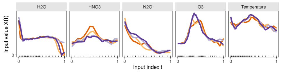
Figure 2: Four sounding input profiles $t_{k}\in[0,1],x_{t_{k}}\in[0,1]$ for $k=1,\dots,K^{(q)}\leq 43,q=1,\dots,Q=5$. Although plotted as lines for ease of access, we observe a finite number of measurements at the locations indicated in the rug.

We define the computer model output $y=6.82^{-1}\left(y^{\textsc{PC1}}-.55\right)\in\mathbb{R}$ with $\operatorname{E}\left[y\right]\approx 0$ and $\operatorname{V}\left[y\right]\approx 1$, where $y^{\textsc{PC1}}\in\mathbb{R}$ denote the MLS Band 2 radiances first multivariate functional principal component score (happ2018), ordered by largest eigenvalue, as produced in related work by johnson2020. All the scaling constants were obtained empirically. The data set is given by the collection $\mathcal{D}={\left\{y_{n},t_{k^{(q)}}^{(q)},x_{n,k^{(q)}}^{(q)}\right\}}_{n,q,k^{(q)}}$.

A total of $16,000$ samples are randomly partitioned into $H=8$ training and $H$ test complementary subsets with $N=1,000$ soundings each. We evaluate the performance of all three ALF models described in Section 2.1. For comparison, we also consider the vector-input Gaussian process (viGP) models viGP-SE with $d_{\textsc{ARD}}(\cdot)$ and $\sigma_{x_{k}}^{2}=\sigma_{x}^{2}>0\ \forall\ k=1,\dots K$; viGP-ARD with $d_{\textsc{ARD}}(\cdot)$ and $\sigma_{x_{k}}^{2}>0\ \forall\ k=1,\dots K$; viGP-FPCA with $d_{\textsc{PC}}(\cdot)$ and $\sigma_{{\tilde{x}}_{\tilde{k}}}^{2}>0\ \forall\ \tilde{k}=1,\dots\tilde{K}_{\textsc{99\%}}$; viGP-FFPCA with $d_{\textsc{PC}}(\cdot)$ and $\sigma_{{\tilde{x}}_{\tilde{k}}}^{2}>0\ \forall\ \tilde{k}=1,\dots,\tilde{K}_{\textsc{full}}$. Models viGP-SE and viGP-ARD have a shared and a separable correlation structure on the vector space respectively. Models viGP-FPCA and viGP-FFPCA have a separable correlation structure on the reduced and full principal component space respectively, the former being restricted to the components accounting for 99% of the input variability. FPCA is set up with a cubic spline smoother, 10 equally-spaced knots in [0, 1], and 12 basis functions, thus $\tilde{K}_{\textsc{full}}=12$. One model is fit separately for each atmospheric input.

Specifying the prior families in Section 2.1, we set the following independent priors: $\phi\sim\textsc{InvGamma}(5,5)$, $\tau\sim\textsc{Beta}(1,1)$, $\smash{{10}^{-\frac{1}{2}}\lambda\sim\textsc{N}^{+}(0,1)}$, $\log(\kappa)\sim\textsc{N}(0,1)$ for the fiGP parameters, $\sigma_{x},\sigma_{x_{k}},\sigma_{{\tilde{x}}_{\tilde{k}}}\smash{\overset{\text{\tiny iid}}{\sim}}\textsc{InvGamma}(5,5)$ for the viGP parameters, and $\sigma_{f},\sigma_{\varepsilon}\smash{\overset{\text{\tiny iid}}{\sim}}\textsc{N}^{+}(0,1)$ for the signal and noise standard deviation parameters. The log posterior is evaluated at 3,000 random locations of the parameter space drawn from $\sigma_{x},\sigma_{x_{k}},\sigma_{{\tilde{x}}_{\tilde{k}}},\phi,5^{-1}\sigma_{f},2\sigma_{\varepsilon}\smash{\overset{\text{\tiny iid}}{\sim}}\textsc{N}^{+}(0,1)$, $\lambda_{1},\lambda_{2}\smash{\overset{\text{\tiny iid}}{\sim}}\textsc{C}^{+}(0,1)$, and $\tau\sim\textsc{Beta}(2/3,1)$. A beta distribution with mean equal to $0.4$ reflects the intuition that input values near ground are expected to have relatively higher predictive relevance. The standard deviations are compatible with the output scale. The multiplicative factors for the standard deviations are motivated by the signal-to-noise ratio $\textsc{STN}=\sigma_{f}/\sigma_{\varepsilon}$ observed in previous exploratory studies. A total of 30 optimizations are initialized at the highest posterior density parameter vectors selected from the 3,000 random candidates. Finally, the optimal values with highest posterior density are used to initialize one MCMC chain with 500 warm-up iterations and $M=1,500$ post warm-up samples. Validation statistics are computed using a sample of $\tilde{M}=100$ thinned observations sampled with a batch size of 150 iterations.

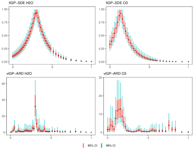
Figure 3: Weight posterior intervals for two models and inputs.

We now discuss the general patterns in the posterior density of the parameter vector $\bm{\theta}$ and the weight function evaluations $\{\omega(t_{k})\}_{k}$, and we then compare the prediction performance across the plausible models. Looking at the ADE parameter posterior expectation across all data subsets in Section 3, a global pattern emerges where the peak relevance $\tau$ is situated in the first half of the index interval. The models posit slowly decaying rates at the left of the peak and an order-of-magnitude faster speed toward the right, i.e., $\lambda_{1}<<\lambda_{2}$. In other words, relevance is higher and relatively more constant near ground while it decreases fast as altitude increases above $\tau$. Consider, for example, Figure 4. With roughly $\operatorname{E}\left[\omega(t)|\mathbf{y}\right]<.05\ \forall\ t>0.5$, the posterior density suggests that differences in H₂O and O₃ near the mesopause have negligible predictive relevance. The parameter posterior density for these are reported in the supplementary material LABEL:app:param-posterior. It might be tempting to interpret the relevance profiles in terms of predictive power (neal1996) and conclude that the chemical composition near the atmospheric edge does not contribute to radiance prediction. However, it is worth cautioning that non-linear terms are also associated with shorter length-scales (piironen2016), and thus the tuned parameters could be partly capturing the fact that the relationship between the radiance and the input is non-linear (“more wiggly”) at lower altitudes and becomes more linear as we ascend over the vertical profile. The standard deviation posterior intervals confirm high signal-to-noise ratios even when the models have only one input variable, with noise contributing less than .05 of the total variance for these two inputs.

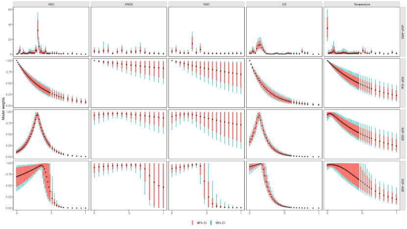
Figure 4: Weight posterior intervals estimated from one data subset. Each model (facet row) is trained to predict radiance as a function of each input variable (facet column)

Model $\tau$ $\lambda_{1}$ $\lambda_{2}$ $\theta$ $\sigma_{\varepsilon}$ $\sigma_{f}$ $\sigma_{f}/\sigma_{\varepsilon}$ $p(\mathbf{\theta}|\mathbf{y})$ $R^{2}$ RMSE Neg. CRPS Neg. PPLD Cov. 95% H2O viGP-SE - - - - .30 (.003) 4.55 (.176) 15.3 (.76) 462 ( 2.3) .89 (.003) .34 (.003) .19 (.001) 273 ( 7.0) .96 (.002) viGP-ARD - - - - .28 (.003) 5.07 (.103) 17.8 (.52) 320 ( 5.4) .91 (.003) .31 (.003) .17 (.001) 196 ( 6.9) .96 (.003) viGP-FPCA - - - - .66 (.009) .63 (.013) 1.0 (.02) -122 ( 9.7) .55 (.010) .67 (.010) .37 (.006) 1024 (14.1) .93 (.003) viGP-FFPCA - - - - .36 (.004) .82 (.010) 2.3 (.03) 256 ( 6.6) .79 (.014) .46 (.015) .25 (.007) 535 ( 6.8) .93 (.006) fiGP-Edn - - 2.40 (.071) .09 (.002) .31 (.003) 6.46 (.152) 21.1 (.73) 419 ( 2.1) .89 (.003) .33 (.004) .18 (.001) 261 ( 7.5) .96 (.002) fiGP-SDE .30 (.001) 7.59 (.193) 7.59 (.193) .06 (.001) .29 (.003) 6.70 (.096) 23.0 (.51) 470 ( 4.9) .91 (.003) .31 (.004) .17 (.001) 202 ( 7.1) .96 (.002) fiGP-ADE .38 (.015) 1.69 (.359) 15.70 (.793) .07 (.002) .29 (.003) 6.60 (.120) 22.7 (.66) 479 ( 5.0) .90 (.003) .31 (.004) .17 (.001) 202 ( 6.5) .96 (.003) HNO3 viGP-SE - - - - .41 (.011) 1.30 (.051) 3.2 (.11) 231 (16.7) .77 (.004) .48 (.005) .26 (.003) 614 (10.4) .95 (.002) viGP-ARD - - - - .43 (.007) 2.77 (.068) 6.5 (.15) 140 (14.3) .78 (.004) .47 (.005) .25 (.003) 619 (11.6) .94 (.003) viGP-FPCA - - - - .90 (.002) .87 (.034) 1.0 (.04) -416 ( 2.3) .19 (.006) .91 (.007) .51 (.004) 1320 ( 7.7) .95 (.004) viGP-FFPCA - - - - .35 (.009) .94 (.014) 2.7 (.08) 150 (14.2) .71 (.007) .54 (.007) .28 (.003) 646 ( 7.7) .95 (.003) fiGP-Edn - - .42 (.080) .12 (.005) .43 (.009) 2.35 (.095) 5.4 (.14) 199 (15.1) .78 (.004) .47 (.005) .25 (.003) 623 (10.9) .95 (.003) fiGP-SDE .29 (.025) .69 (.175) .69 (.175) .12 (.005) .43 (.009) 2.39 (.105) 5.5 (.17) 198 (15.0) .78 (.004) .47 (.005) .25 (.003) 623 (10.9) .95 (.003) fiGP-ADE .62 (.013) .22 (.017) 24.13 ( 3.011) .12 (.006) .43 (.007) 2.58 (.116) 6.0 (.21) 204 (14.2) .78 (.003) .47 (.005) .25 (.003) 610 (11.2) .95 (.003) N2O viGP-SE - - - - .42 (.004) 1.04 (.043) 2.5 (.10) 291 ( 9.8) .81 (.004) .44 (.005) .24 (.002) 585 (10.3) .94 (.002) viGP-ARD - - - - .42 (.004) 1.93 (.074) 4.6 (.17) 194 ( 9.8) .81 (.004) .43 (.005) .24 (.002) 581 (11.0) .94 (.001) viGP-FPCA - - - - .97 (.005) .53 (.020) .5 (.02) -484 ( 5.1) .04 (.006) .99 (.008) .56 (.004) 1406 ( 7.9) .94 (.003) viGP-FFPCA - - - - .41 (.004) .64 (.008) 1.6 (.02) 160 ( 9.1) .79 (.008) .46 (.009) .25 (.004) 630 (12.9) .94 (.003) fiGP-Edn - - .66 (.066) .14 (.002) .43 (.004) 2.30 (.074) 5.4 (.18) 261 ( 9.6) .81 (.004) .44 (.005) .24 (.002) 585 (10.6) .94 (.001) fiGP-SDE .24 (.018) .75 (.063) .75 (.063) .14 (.003) .43 (.004) 2.26 (.073) 5.3 (.19) 259 ( 9.6) .81 (.004) .44 (.005) .24 (.002) 585 (10.6) .94 (.001) fiGP-ADE .43 (.005) .35 (.043) 28.19 ( 2.163) .13 (.003) .43 (.004) 2.53 (.061) 5.9 (.16) 266 ( 9.7) .81 (.004) .43 (.005) .24 (.002) 581 (11.0) .94 (.001) O3 viGP-SE - - - - .24 (.004) 6.02 (.244) 25.4 ( 1.11) 540 ( 7.4) .90 (.004) .32 (.007) .17 (.003) 138 (10.1) .97 (.002) viGP-ARD - - - - .24 (.003) 6.85 (.140) 28.8 (.73) 387 ( 9.9) .91 (.002) .30 (.003) .16 (.001) 92 ( 8.7) .96 (.001) viGP-FPCA - - - - .45 (.004) 1.19 (.052) 2.7 (.12) 260 (10.9) .79 (.003) .46 (.006) .25 (.002) 637 (13.0) .93 (.002) viGP-FFPCA - - - - .24 (.004) .83 (.014) 3.5 (.09) 489 ( 9.9) .86 (.004) .38 (.006) .20 (.003) 295 (11.2) .96 (.001) fiGP-Edn - - 4.02 (.143) .07 (.001) .25 (.004) 8.22 (.137) 33.6 (.83) 528 ( 8.9) .92 (.003) .29 (.004) .16 (.002) 90 ( 9.0) .96 (.002) fiGP-SDE .14 (.002) 7.17 (.390) 7.17 (.390) .07 (.001) .25 (.004) 8.21 (.154) 33.2 (.82) 543 (10.3) .92 (.002) .29 (.004) .15 (.002) 85 ( 8.9) .96 (.002) fiGP-ADE .24 (.031) .48 (.062) 10.59 (.621) .07 (.003) .25 (.004) 8.16 (.158) 33.0 (.94) 553 (10.5) .92 (.002) .29 (.004) .16 (.001) 87 ( 8.7) .96 (.003) Temperature viGP-SE - - - - .21 (.003) 1.27 (.034) 5.9 (.15) 798 ( 9.3) .94 (.001) .25 (.002) .14 (.001) -7 ( 1.6) .97 (.003) viGP-ARD - - - - .23 (.003) 2.82 (.030) 12.5 (.20) 559 ( 8.4) .94 (.001) .25 (.002) .14 (.001) -13 ( 3.7) .96 (.002) viGP-FPCA - - - - .53 (.009) 1.07 (.031) 2.0 (.09) 85 (16.6) .71 (.008) .54 (.008) .29 (.003) 802 (14.5) .94 (.004) viGP-FFPCA - - - - .28 (.005) .76 (.013) 2.7 (.09) 467 (10.2) .89 (.001) .33 (.002) .18 (.001) 268 ( 7.2) .96 (.003) fiGP-Edn - - 1.31 (.129) .08 (.003) .23 (.003) 2.94 (.094) 12.8 (.39) 729 ( 8.9) .94 (.001) .25 (.003) .14 (.001) 4 ( 5.3) .96 (.002) fiGP-SDE .08 (.015) 1.39 (.151) 1.39 (.151) .08 (.003) .23 (.003) 2.92 (.106) 12.8 (.43) 726 ( 8.9) .94 (.001) .25 (.003) .14 (.001) 4 ( 5.4) .96 (.003) fiGP-ADE .34 (.030) .35 (.096) 3.09 (.429) .08 (.003) .23 (.003) 2.86 (.096) 12.6 (.37) 729 ( 9.1) .94 (.002) .25 (.003) .14 (.002) 2 ( 5.2) .96 (.003)

Table 1: Tuned model parameters and validation statistics across five input variables (line-separated table sections) and plausible models (rows). Each cell reports the mean across the subset means $\bar{v}^{(p,q)}$ and the corresponding standard error $\textsc{SE}\left(\bar{v}^{(p,q)}\right)$ in parenthesis. Bold values are the best in class.

It is also of interest to compare the posterior intervals for the SDE and ARD weights, i.e., $\omega(t_{k})$ versus $\sigma_{x_{k}}^{-2}$ over $k$. The latter offers full flexibility at the price of $K^{(q)}/3<14$ times more tuning parameters. In Figure 3, we observe that both the parametric and the fully separable weights estimate the highest relevance index region in the same neighborhood. For H₂O, $\operatorname*{arg\,max}_{k}\operatorname{E}\left[\sigma_{x_{k}}^{-2}|\mathbf{y}\right]=20$ with $t_{20}=.31$, and $\operatorname{E}\left[\tau|\mathbf{y}\right]=.30$ with $P(.27\leq\tau\leq.32|\mathbf{y})=.95$. Similarly for O₃, $\operatorname*{arg\,max}_{k}\operatorname{E}\left[\sigma_{x_{k}}^{-2}|\mathbf{y}\right]=9$ with $t_{9}=.16$, and $\operatorname{E}\left[\tau|\mathbf{y}\right]=.13$ with $P(.11\leq\tau\leq.16|\mathbf{y})=.95$. The ARD weights are locally higher near the maximum and vary rather smoothly across $k$, just as assumed by ALF. However, posterior uncertainty in the relevance profiles manifest rather homogeneously over the index space for SDE whereas ARD exhibits increased uncertainty around the relevance peak with a coefficient of variation 5 times larger than in SDE (.06 and .32 respectively).

The validation statistics $\mathcal{V}=\left\{\bar{v}^{(p,q)}\right\}$ are summarized in LABEL:tab:validation-statistics-mini. See Sections 3 and LABEL:fig:validation-foldmeans-brief in the supplementary material for a detailed report of in and out-of-sample statistic means and standard errors. The across-input means $\bar{v}^{(p)}=5^{-1}\sum_{q=1}^{5}\bar{v}^{(p,q)}$ suggest that the ALF models perform similarly to the viGP models with no input pre-processing. For most purposes, there is a negligible edge for SDE and ADE over Edn, and ARD over SE. With the aid of Section 3, we observe that this difference is slightly more favorable for H₂O and Temperature. Overall, the ADE and ARD models are arguably a sensible choice across this study combinations. In most situations, it is also reasonable to argue for the SDE variant given the similar predictive quality and parsimony. The coefficient of determination and the negative CRPS produce similar findings to the RMSE and the negative PPLD, as expected given that these quantities are intrinsically related. Coupling ADE or ARD with temperature produces the highest coefficient of determination .94, the smallest RMSE .25, and CRPS .14 and the best PPLD. As a general note, the actual mean coverage of the point-wise predictive interval is close to its nominal value in most cases. For all inputs, FFPCA performs worse than ARD and fiGP. Additionally, FFPCA’s RMSE is 17-54% smaller than FPCA’s, which retains 99% of the explained variation. This is yet another illustration that variability in the input space need not relate with predictive power.