Minimum Flow Decomposition in Graphs with Cycles
using Integer Linear Programming

Abstract

Minimum flow decomposition (MFD) — the problem of finding a minimum set of weighted source-to-sink paths that perfectly decomposes a flow — is a classical problem in Computer Science, and variants of it are powerful models in a different fields such as Bioinformatics and Transportation. Even on acyclic graphs, the problem is NP-hard, and most practical solutions have been via heuristics or approximations. While there is an extensive body of research on acyclic graphs, currently there is no exact solution on graphs with cycles. In this paper we present the first ILP formulation for three natural variants of the MFD problem in graphs with cycles, asking for a decomposition consisting only of weighted source-to-sink paths or cycles, trails, and walks, respectively. On three datasets of increasing levels of complexity from both Bioinformatics and Transportation, our approaches solve any instance in under 10 minutes. Our implementations are freely available at github.com/algbio/MFD-ILP.

1 Introduction

1.1 Background

Flow decomposition (FD) is a classical and well-researched network problem in which a source-to-sink flow needs to be decomposed into a set of weighted source-to-sink paths (and possibly cycles) such that their respective weights perfectly fit each edge’s flow. An essential textbook property (see, e.g.  (Ahuja et al.,, 1988)) is that any flow in a graph with $m$ edges can be decomposed into at most $m$ paths or cycles (each with some associated weight). However, some flow paths or cycles could be suitably combined to form a smaller decomposition. Therefore, a popular and practically-motivated variant of the flow decomposition problem is to find the decomposition into the minimum amount of paths or cycles (Minimum Flow Decomposition problem, MFD). This variant, however, is NP-hard, even if the input network is restricted to a directed acyclic graph (DAG), as first observed by Vatinlen et al., (2008).

Despite their NP-hardness, MFD and its variants are used in many applications, such as computer networking (Mumey et al.,, 2015; Hartman et al.,, 2012; Cohen et al.,, 2014; Hong et al.,, 2013), Transportation science (Olsen et al.,, 2020; Ohst,, 2015), and bioinformatics (Dias et al.,, 2022; Kovaka et al.,, 2019; Kloster et al.,, 2018; Zhang et al.,, 2021; Sashittal et al.,, 2021). The input graph may naturally be a DAG in some applications, such as reference-based RNA transcript assembly in bioinformatics. However, in many applications, the input network graph naturally contains cycles, as in computer and transportation networks, or sequence assembly problems from bioinformatics (Grabherr et al.,, 2011; Schulz et al.,, 2012).

Despite the need to decompose flows with cycles in applications, much of the recent progress on MFD has focused on DAGs, due to properties associated with acyclicity that can be exploited into algorithms, as in the fixed-parameter tractable (FPT) algorithms of Kloster et al., (2018) and Williams et al., (2021), the integer linear programming (ILP) formulation of Dias et al., (2022), and the heuristic algorithm called Catfish (Shao and Kingsford, 2017b, ).

In fact, no exact (that is, returning a truly minimum solution) solver exists for MFD on graphs with cycles. Because different applications may require different types of decompositions, in this paper, we study three natural versions of the problem on cyclic inputs: decomposing into source-to-sink paths or cycles (in this paper, paths and cycles do not repeat nodes, except for cycles where the first and last nodes are the same), into source-to-sink trails (which may repeat nodes but not edges), and into source-to-sink walks (which may repeat both nodes and edges).

1.2 Related Work

The MFD problem was first formally studied in (Vatinlen et al.,, 2008), where it was shown to be NP-hard, even on DAGs. This result was later strengthened by Hartman et al., (2012), who proved several additional results for the problem. They showed that the problem is also NP-hard when the flow values come from only the set $\{1,2,4\}$, that MFD is hard to approximate (i.e., there is some $\epsilon>0$ such that MFD cannot be approximated within a $(1+\epsilon)$ factor, unless P=NP), even on DAGs. On the positive side, on DAGs, it is possible to decompose all but a $\varepsilon$-fraction of the flow within a $O(1/\varepsilon)$ factor of the optimal number of paths. Mumey et al., (2015) gave an approximation algorithm for DAGs with an exponential approximation factor based on decomposing the flow into paths with weights that are powers of two. Recently, Cáceres et al., (2022) showed that if the weights of the flow decomposition paths can also take negative integer values, then a polynomial-time approximation algorithm exists for DAGs, with an approximation factor of $\lceil\log||f||\rceil+1$, where $||f||$ is the largest flow value of any edge. Additionally, Kloster et al., (2018) showed that the problem on DAGs is FPT in the size of the minimum decomposition.

In practice, though, applications tend to use heuristics, such as the greedy methods based on choosing the widest or longest paths (Vatinlen et al.,, 2008), and these heuristics can be applied to both DAGs and general graphs, possibly with cycles. Some of these greedy methods could be improved on DAGs by making iterative modifications to the flow graph before finding a greedy decomposition, as shown by Shao and Kingsford, 2017b . However, Cáceres et al., (2022) also showed that there exist some instances (even DAGs) where the MFD has size $O(\log m)$ ($m$ is the number of edges of the graph), where such greedy methods return flow decompositions as large as $\Omega(m/\log m)$, meaning that they can be exponentially worse than the optimum.

Many application-oriented algorithms on DAGs for MFD and related problems use ILP, taking advantage of existing software such as Gurobi (Gurobi Optimization, LLC,, 2021) and CPLEX (Studio,, 2017). However, most of these solutions encode every possible source-to-sink path as a variable, yielding exponential-size ILP formulations that are impractical to solve for larger instances, which occur in applications such as computer networking (Cohen et al.,, 2014). A common strategy amongst bioinformatics applications to deal with this issue is to pre-select some subset of the possible paths in the graph, either for all instances (as in vg-flow (Baaijens et al.,, 2020) and CLIIQ (Lin et al.,, 2012)), or only when the input is extensive (as in MultiTrans (Zhao et al.,, 2021) and SSP (Safikhani et al.,, 2013)). However, by pre-selecting only some paths that can be part of a solution, these algorithms may return a non-optimal decomposition.

Recently, two polynomial-size ILP formulations have been proposed that can be used to solve MFD on DAGs without pre-selecting paths. Namely, the program JUMPER (Sashittal et al.,, 2021) requires an additional condition on the input DAG, namely that it has a unique Hamiltonian path. This allows all paths to be uniquely determined by subsets of edges that do not pairwise overlap along the Hamiltonian path, yielding a formulation for decomposing into $k$ paths using only a quadratic number of variables and constraints. In Dias et al., (2022), the authors give a general solution working on any DAG to find a size $k$ decomposition, even without a Hamiltonian path, again using only a quadratic number of variables and a linear number of constraints. There, the insight is that source-to-sink paths can be encoded using conservation of flow constraints, as in Taccari, (2016). However, neither of these approaches can be straightforwardly extended to handle non-DAG inputs.

As outlined above, most of the contributions to the flow decomposition problem have been restricted to DAGs, the only attempts for the general cyclic case that we know of being limited to heuristics. Since these heuristics can be exponentially worse than the optimum (as discussed above), the quest for efficient and exact MFD approaches to the cyclic case is wide open.

1.3 Our contributions

In this paper, we give the first exact solutions for MFD on graphs with cycles, based on ILP, for all three natural variants mentioned in Section 1.1. In addition, we show that our solutions are also efficient through experiments on three datasets from two application domains, Bioinformatics and Transportation Science.

While our solutions follow the same high-level approach from (Dias et al.,, 2022) when solving MFD on DAGs (i.e., first model each of the $k$ paths by an auxiliary unit flow and then requires that these paths admit weights so that they form a flow decomposition), the cyclic case poses several difficulties, which we overcome as follows.

As a major novelty, in this paper, we show how to formulate different types of walks in graphs with cycles (i.e., paths or cycles, trails, walks) using ILP. The simple path-modelling techniques from (Dias et al.,, 2022) heavily rely on the acyclicity of the graph; thus, here, we need to develop new techniques. Another difficulty we overcome is that trails can visit nodes multiple times, and walk can visit both nodes and edges multiple times. Apart from complicating the modelling, these facts also render some constraints more challenging to linearize than in (Dias et al.,, 2022). Our solutions can be summarized as follows:

• For the paths or cycles variant, we extend the so-called “sequential formulation” of Miller et al., (1960) (see also (Taccari,, 2016)) to uniformly model either a path or a cycle (i.e., by a single set of variables with associated constraints). We still model them by an auxiliary unit flow but add new constraints to require that this auxiliary flow induces either a path or a cycle.

• For the trails and walks variants, we give a novel reachability-based formulation characterizing when the auxiliary unit flow corresponds to a trail or to a walk, as follows. In order to model a source-to-sink walk, more than simply modelling a unit flow is required because in graphs with cycles, and it may induce isolated strongly connected components. Thus, we add constraints to require that any node incident to the unit flow modelling the walk is reachable from the source via a spanning tree rooted at the source and using edges of the unit flow.

• For the trails variant, we also propose an alternative approach that forbids such isolated strongly connected components via an iterative constraint generation procedure. This approach is inspired by previous constraint generation approaches from (Dantzig et al.,, 1954; Taccari,, 2016). However, these previous approaches model paths by forbidding only cycles (since a unit flow induces a path if and only if it contains no cycles). Trails and walks can contain cycles, so we need to forbid entire strongly connected components.

All the formulations are of quadratic size in the number of constraints and variables, except for the constraint generation approach, which introduces several linear constraints in the graph’s number of edges per iteration.

Our ILPs constitute the first exact solutions for the NP-hard MFD problem on graphs with cycles for its three natural variants on such inputs. At the same time, we also show that they are efficient with biological and transportation data from different sources, solving simple instances in under 60 seconds and more complex ones in under 12 minutes. Lastly, mathematical programming can provide significant flexibility that is not easy to incorporate in purely algorithmic formulations. In fact, our ILP formulations can be easily extended to practical aspects of applications. This can be done either by suitably adapting the formulation of what constitutes an element of a decomposition (here, we extended paths to paths or cycles, trails, and walks) or by adapting the condition of when the weighted paths fit the flow edges (for example, by considering inexact, or imperfect flow decomposition as in (Williams et al.,, 2019) and (Dias et al.,, 2022)).

The paper is organized as follows. We review the basic concepts of flow networks and flow decomposition and define the problems addressed in Section 2. We next present the ILP models for each problem variant, starting with paths or cycles in Section 3.1, trails in Section 3.2, and walks in Section 3.3. Numerical experiments are provided in Section 4, and concluding remarks are discussed in Section 5.

2 Preliminaries

2.1 Basic notions

In this paper, by a graph $G=(V,E)$, we mean a directed graph with $E\subseteq V\times V$. We also assume that all graphs are weakly connected in the sense that there is an undirected path between any pair of nodes. A source of $G$ is a node without incoming edges, and a sink is a node without outgoing edges. We will use $n$ and $m$ to denote the cardinality of the sets of nodes V and edges E, respectively, of the graph.

A walk in $G$ in a sequence of edges in $E$ where consecutive edges share an end and a start. Given a walk $W$ in $G$, and an edge $(u,v)$ of $G$, we denote by $W(u,v)$ the number of times $W$ passes through $(u,v)$ (and thus 0 if $W$ does not pass through $(u,v)$). We say that $W$ is a trail if $W(u,v)=1$ for all edges $(u,v)$ in $W$. We say that $W$ is a path if $W$ repeats no node, and that $W$ is a cycle if $W$ repeats no node, with the exception that the first and the last node are the same. If $W$ has first node $s$ and last node $t$, we say that $W$ is an $s$-$t$ walk (or $s$-$t$ trail, or $s$-$t$ path, accordingly). A strongly connected component of $G$ is an inclusion-maximal set $C$ of nodes of $G$ such that for any $x,y\in C$, there is an $x$-$y$ path, and an $y$-$x$ path.

2.2 Network flows and flow decompositions

Definition 1 (Flow network)

A tuple $G=(V,E,f)$ is said to be a flow network if $(V,E)$ is a graph with unique source $s$ and unique sink $t$, where for every edge $(u,v)\in E$ we have an associated positive integer flow value $f_{uv}$, satisfying conservation of flow for every $v\in V\setminus\{s,t\}$, namely:

$$\sum_{(u,v)\in E}f_{uv}=\sum_{(v,w)\in E}f_{vw}.$$ (1)

Next, we define when a set of generic walks in a flow network form a flow decomposition. By considering different types of walks, we will obtain the specific problem variants of this paper.

Definition 2 ($k$-Flow Decomposition)

A $k$-flow decomposition $(\mathcal{W},w)$ for a flow network $G=(V,E,f)$ is a set of $k$ walks $\mathcal{W}=(W_{1},\ldots,W_{k})$ in $G$ and associated weights $w=(w_{1},\ldots,w_{k})$, with each $w_{i}\in\mathbb{Z}^{+}$, such that for each edge $(u,v)\in E$ it holds that:

$$\sum_{i\in\{1,\dots,k\}}w_{i}W_{i}(u,v)=f_{uv}.$$ (2)

The number $k$ of walks is also called the size of the flow decomposition.

We will consider several types of walks, and obtain corresponding variants of the flow decomposition problem (see also Figure 1). We will also refer to the walks of a decomposition as its elements. Next, we define the flow decomposition problems by asking for decompositions into at most $k$ elements.

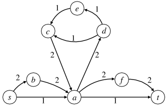
(a)

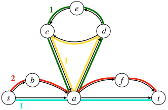
(b)

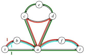
(c)

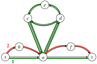
(d)

Figure 1: Example of a flow network (1(a)) and of three different types of minimum flow decomposition into paths or cycles (1(b)), trails (1(c)) and walks (1(d)).

t

Definition 3 ($k$-Flow Decomposition Problems)

Given a flow network $G=(V,E,f)$, consider the problem of finding a flow decomposition into at most $k$ walks and associated weights. If these walks are required to be:

• $s$-$t$ paths or cycles, then we call the resulting problem $k$-Flow Decomposition into Paths or Cycles ($k$-FDPC);

• $s$-$t$ trails, then we call the resulting problem $k$-Flow Decomposition into Trails ($k$-FDT);

• $s$-$t$ walks, then we call the resulting problem $k$-Flow Decomposition into Walks ($k$-FDW).

It is a standard result (see e.g. Ahuja et al., (1988)) that any flow network can be decomposed into paths or cycles because one can consider any edge $(u,v)$, and by conservation of flow, extend this edge in both directions either into an $s$-$t$ path, or into a cycle, associate weight $1$ to it, and remove it from the flow network, obtaining another flow network. We can analogously deduce that any flow network can also be decomposed into a collection of $s$-$t$ walks. The simplest proof of this fact can be obtained by creating another graph by replacing every edge $(u,v)$ with $f(u,v)$ parallel edges and adding as many parallel edges from $t$ to $s$ as there is flow out-going from $s$. Since in this graph, every node has as many in-neighbours as out-neighbours (by construction and by conservation of flow), the resulting graph has an Eulerian walk with the first and last node equal to $s$. Every time this walk passes through one of the parallel edges from $t$ to $s$ we cut it by removing such edges. The resulting pieces are $s$-$t$ walks covering all edges, thus forming a flow decomposition of the original graph, where each walk is associated with weight 1.

However, not all flow networks admit flow decomposition into $s$-$t$ trails. For example, this is the case for the flow network made up of edges $(s,a),(a,d),(d,c),(c,a),(a,t)$, with flow values $f(s,a)=1$, $f(a,d)=2$, $f(d,c)=2$, $f(c,a)=2$ and $f(u,t)=1$ (see also Figure 2).

Figure 2: Example of a network that does not admit a decomposition into $s$-$t$ trails.

In practice, we are interested in decompositions of minimum size (i.e., with the minimum number of elements, that is, walks, recall Definition 2). As such, we can introduce the minimization version of each problem, as follows.

Definition 4 (Minimum Flow Decomposition (MFD))

For each of the problems $k$-FDPC, $k$-FDT, $k$-FDW, its minimization version asks finding a flow decomposition of minimum size (i.e., minimizing $k$).

All our ILP formulations will assume at most $k$ paths/cycles, trails, or walks. As such, the minimization versions of the problems can be solved via an iterative process, trying all possible $k$ in increasing order until reaching the minimum size $k^{\ast}$ of a decomposition (or $m$, which is an upper bound on the size of an MFD in all problem variants, as discussed above). When $k>m$, it means that there is no feasible solution. This iterative approach leads to $k^{\ast}$ runs of our ILPs.

However, a more efficient approach, leading to only $O(\log k^{\ast})$ runs of our ILPs, is based on the fact that if a decomposition of size at most $k$ exists, then trivially also one of size at most $k^{\prime}>k$ exists as well. As such, we can first do a doubling (or exponential) approach (Bentley and Yao,, 1976) by running our ILPs with $k=1,2,4,\dots$, until finding the smallest $k$ such that a decomposition of size at most $2k$ exists, but one of size $k$ does not exists. Then, it holds that $k^{\ast}\in(k,2k]$, and we can find $k^{\ast}$ with a binary search in this interval.

2.3 ILP formulation of $s$-$t$ paths in DAGs and of flow decompositions

In this section we review the formulation from Taccari, (2016) of an $s$-$t$ path in a graph $G=(V,E)$, with $s,t\in V$, and then recall the use of this formulation in the ILP solution for MFD in DAGs (Dias et al.,, 2022).

For every edge $(u,v)\in E$, we can introduce a binary variable $x_{uv}$. The idea is to represent the $s$-$t$ path by the edges $(u,v)$ having $x_{uv}=1$. If $G$ is a DAG, it suffices to impose the following constraint, stating that the $s$-$t$ path starts with a single edge out-going from $s$, ends with a single edge in-coming to $t$, and at every other node $v$, either it does not pass through the node, or if it reaches $v$, it also exits $v$. Note that since $G$ is a DAG, no walk can use a node $v$ multiple times.

$$\sum_{(u,v)\in E}x_{uv}-\sum_{(v,u)\in E}x_{vu}=\begin{cases}0,&\text{if $v\in V\setminus\{s,t\}$},\\ 1,&\text{if $v=t$},\\ -1,&\text{if $v=s$}.\end{cases}$$ (3)

We will refer to the above constraint as the “flow conservation” constraint (not to be mistaken with the conservation of the input flow). In Dias et al., (2022), a flow decomposition in DAGs into exactly $k$ $s$-$t$ paths is expressed by adding $k$ copies of the above variables, namely $x_{uvi}$, for $i\in\{1,\dots,k\}$, and imposing the flow conservation constraint (3) for all of them. The flow decomposition constraint (2) can be stated as

$$\sum_{i\in\{1,\dots,k\}}x_{uvi}w_{i}=f_{uv}, \forall(u,v)\in E.$$ (4)

We refer to this ILP formulation for MFD in DAGs as the standard formulation; our formulations will build on this, mainly by possibly changing Eq. 3 and adding further constraints to the $x_{uvi}$ variables to model all types of walks considered in this paper.

Remark 1

The constraint in Eq. (4) can be linearized by introducing an integer variable $\pi_{uvi}$ representing the product $x_{uvi}w_{i}$, together with the following constraints, where $M$ is any constant strictly greater than the right-hand side of the first inequality (Soltysik and Yarnold, (2010)) in Eq. (5b):

$$f_{uv}=\sum_{i\in\{1,\dots,k\}}\pi_{uvi}, \forall(u,v)\in E,$$ (5a)

$$\pi_{uvi}\leq Mx_{uvi}, \forall(u,v)\in E,\forall i\in\{1,\dots,k\},$$ (5b)

$$\pi_{uvi}\leq w_{i}, \forall(u,v)\in E,\forall i\in\{1,\dots,k\},$$ (5c)

$$\pi_{uvi}\geq w_{i}-(1-x_{uvi})M, \forall(u,v)\in E,\forall i\in\{1,\dots,k\}.$$ (5d)

Indeed, in inequality (5b), for $x_{uvi}=1$, the constraint should be bounded by the flow value $f_{uv}$. If $x_{uvi}=0$, then the constraint is not binding, therefore the left side can be any value that is smaller or equal to zero. For constraint (5d), when $x_{uvi}=1$, the value of $M$ is irrelevant; when $x_{uvi}=0$, the constraint is not binding as long as $M$ is a positive number. Therefore, the best value of $M$ is $M=f_{uv}$.

3 ILP Formulations for MFD in Graphs with Cycles

3.1 $k$-Flow Decomposition into Paths or Cycles

In this section we tackle the $k$-FDPC problem. We start as in the standard formulation, by using the same binary variables $x_{uvi}$ for every edge $(u,v)\in E$ and every $i\in\{1,\dots,k\}$. Since paths and cycles can visit any node at most once, we adapt the flow conservation constraint (3) into the following constraints:

$$\sum_{(u,v)\in E}x_{uvi}\leq 1 \forall u\in V,\forall i\in\{1,\ldots,k\},$$ (6a)

$$\sum_{(u,v)\in E}x_{uvi}-\sum_{(v,w)\in E}x_{vwi}=0 \forall i\in\{1,\ldots,k\},\forall v\in V\setminus\{s,t\}.$$ (6b)

However, if $G$ is not a DAG, the binary variables $x_{uvi}$ could for example induce an $s$-$t$ path and one or more cycles (not even reachable from the $s$-$t$ path).

To overcome this, we start from a formulation of an $s$-$t$ path in general graphs, presented in Taccari, (2016) as the sequential formulation, and attributed to Miller et al., (1960). This formulation introduces a positive integer variable $d_{v}$ for every node $v\in V$, which will stand for the position of $v$ in the path. The following constraint is introduced for every edge:

$$d_{v}\geq d_{u}+1+(n-1)(x_{uv}-1) \forall(u,v)\in E.$$ (7)

This assigns a partial order to the nodes, such that for any edge $(u,v)$ with $x_{uv}=1$, we have $d_{u}<d_{v}$. We can also think of the $d_{v}$ variables as a pseudo-distance function, where the true distance from $s$ to $t$ is obtained by minimizing $d_{t}$. However, constraint (7) as is forbids cycles altogether, which is not the goal in the $k$-FDPC problem.

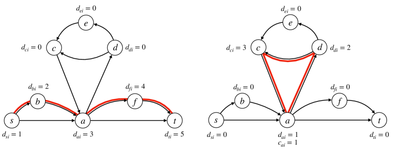
Figure 3: Example of the edge variables $x_{uvi}$ (where we draw edge $(u,v)$ in red if $x_{uvi}=1$, and in black otherwise), satisfying Eqs. 6b and 6a. On the left, the assignments of the variables $d_{vi}$ shown in the figure (and $c_{vi}=0$ for all $v\in V$) satisfy constraint (8). On the right, the assignments of the variables $d_{vi}$ shown in the figure (and $c_{vi}=1$ for all $v\in V\setminus\{a\}$, and $c_{ai}=1$) satisfy constraint (8). Note that the only edge $(u,v)$ such that $d_{vi}<d_{ui}$ is $(c,a)$. However, constraint (8) holds for $(c,a)$ because $c_{ai}=1$.

In order to handle both paths and cycles, we modify the sequential formulation constraint (7) as follows. For every $v\in V\setminus\{s,t\}$, we introduce a binary variable $c_{vi}$ to denote whether node $v$ is a “start of cycle” node in the $i$-th element of the flow decomposition. We also introduce positive integer variables $d_{vi}$, and change (7) into the following constraint:

$$d_{vi}\geq d_{ui}+1+(n-1)(x_{uvi}-1-c_{vi}) \forall(u,v)\in E,\forall i\in\{1,\ldots,k\}.$$ (8)

Namely, this constraint imposes that either a node is the starting point of a cycle or its order in the path is always increasing. Finally, we impose:

$$\sum_{v\in V}x_{svi}+\sum_{v\in V}c_{vi}\leq 1 \forall i\in\{1,\dots,k\}.$$ (9)

That is, for every element $i$ of the decomposition, either there is some edge $(s,v)$ with $x_{svi}=1$ (in which case we have just an $s$-$t$ path, and no cycle), or $c_{vi}=1$ for some $v$ (or none of these hold) (see Figure 3). Because of constraint (6b), if $\sum_{v\in V}x_{svi}=1$, then the binary $x_{uvi}$ variables induce just an $s$-$t$ path and no other cycles. If $c_{vi}=1$, this means that we have no $s$-$t$ path and just one cycle (or none at all, if all $x_{uvi}$ variables are zero). Finally, observe that adding constraint (9) we obtain that constraint (6a) is always satisfied, since otherwise, we have either at least two $s$-$t$ paths passing through $u$ in some element $i$ of the decomposition (and thus $\sum_{v\in V}x_{svi}\geq 2$), or two cycles passing through $u$ in some element $i$ of the decomposition (and thus $\sum_{v\in V}c_{vi}\geq 2$).

The complete ILP formulation for this problem variant, which we give as Model 26 in A, has $O((|V|+|E|)k)$ variables and constraints.

Remark 2

The formulation for $k$-FDPC presented here is capable of decomposing the flow into up to $k$ paths or cycles. However, one can easily obtain a formulation where there are exactly $k$ elements in the decomposition, as follows. The constraint in (9) allows the number of total cycles and paths to be up to $k$, by allowing either terms of the left-hand side to be at most 1. Therefore, this constraint needs to be changed to:

$$\sum_{v\in V}x_{svi}+\sum_{v\in V}c_{vi}=1 \forall i\in\{1,\dots,k\}.$$ (10)

3.2 $k$-Flow Decomposition into Trails via Constraint Generation

In this section we tackle the next problem, $k$-FDT, namely finding a $k$-flow decomposition into at most $k$ $s$-$t$ trails. Recall from the previous sections that the binary $x$ variables induce a flow. The only case when such flow does not correspond to an $s$-$t$ trail is when it has a strongly connected component that is not reachable from $s$, or equivalently, that does not reach $t$.

We start with a simple lemma stating that, due to flow conservation, this global reachability property can be reduced to checking whether any strongly connected component $C$ induced by the edges of the trail has an edge out-going from $C$ (i.e., an edge $(u,v)$ with $x_{uvi}=1$, such that $u$ appears in $C$, but $(u,v)$ does not belong to $C$). For a strongly connected component $C$ of $G$, we denote by $E(C)$ the set of edges of $C$ and by $\delta^{+}(C)$ the set of edges $(u,v)$ such that $u$ belongs to $C$.

Lemma 1

Let $G=(V,E)$ be an arbitrary graph with source and sink nodes $s$ and $t$. Let $W$ be a set of edges of $G$, where for every edge $(u,v)\in E$ we define $W(u,v):=1$, if $(u,v)\in W$, and $W(u,v):=0$ otherwise. It holds that the edges of $W$ can be ordered to obtain a $s$-$t$ trail passing through each edge of $W$ if and only if the following conditions hold:

1. For every $v\in V$, $\displaystyle\sum_{(u,v)\in E}W(u,v)-\sum_{(v,u)\in E}W(v,u)=\begin{cases}0,&\text{if $v\in V\setminus\{s,t\}$},\\ 1,&\text{if $v=t$},\\ -1,&\text{if $v=s$}.\end{cases}$

2. For any strongly connected component $C$ of the subgraph of $G$ induced by the edges in $W$ and different from $\{t\}$, $\delta^{+}(C)\setminus E(C)\cap W$ is non-empty.

Proof 1

For the forward implication, suppose the edges of $W$ can be ordered to obtain an $s$-$t$ trail $T$ that satisfies condition 1. To see that $W$ satisfies also condition 2., let $C$ be a strongly connected component of the subgraph of $G$ induced by the edges of $W$, different from $\{t\}$. First, note that node $t$, being a sink, does not belong to $C$.

If $C$ contains a single node, say $v\neq t$, then the edge of the trail out-going from $v$ belong to $\delta^{+}(C)\setminus E(C)\cap W$. Otherwise, let $(u,v)$ be the edge of $C$ that is last in the order given by the trail $T$. Say that $(v,w)$ is the edge following $(u,v)$ in $T$ (which exists because $v\neq t$). We have that $(v,w)\in\delta^{+}(C)$ (since $v$ belong to $C$), $(v,w)\notin E(C)$ (since $(u,v)$ is the last edge of $C$ in the order given by $T$, and $(u,v)\in W$, since $(u,v)$ is an edge of the trail. Thus, the set $\delta^{+}(C)\setminus E(C)\cap W$ is non-empty, and $W$ satisfies Condition 2.

For the reverse implication, suppose $W$ satisfies the two conditions. Since the values $W(u,v)$ induce a flow in $G$, it remains to prove that this flow is decomposable into a single $s$-$t$ trail. Since $\sum_{(u,t)\in E}W(u,t)-\sum_{(t,u)\in E}W(s,u)=1$, the only way this does not hold is when $W$ also contains a set of edges forming a strongly connected component, and no node in this component reaches $t$. This means that all edges out-going from the nodes of $C$ are to other nodes of $C$ (by flow conservation, and by the fact that $t$ is not reachable from $C$). However, this contradicts the second condition. See the example in Figure 4.

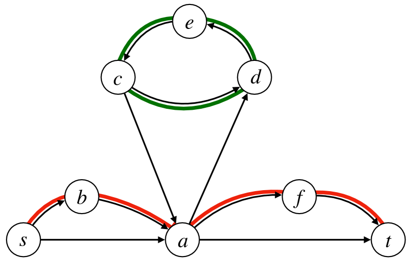
(a) $W_{1}$

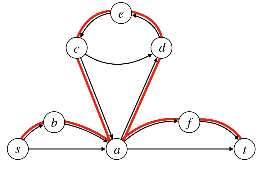
(b) $W_{2}$

Figure 4: The graph from Figure 1, with the edge $(d,c)$ reversed. This creates the cycle $(c,d,e,c)$ in the graph, which can lead to a set $W_{1}$ of edges (on the left, with edges in both red and green), satisfying condition 1. of Lemma 1, but with a strongly connected component (in green) violating condition 2. of Lemma 1. Instead, the set $W_{2}$ (on the right, with edges in red) satisfies both conditions of Lemma 1.

As in the standard formulation, for every edge $(u,v)\in E$ and for every $i\in\{1,\dots,k\}$, we introduce a binary variable $x_{uvi}$ that will equal 1 if and only if the $s$-$t$ trail $W_{i}$ passes through $(u,v)$ (since trails can also visit edges at most once). The first condition of Lemma 1 is the same as the flow conservation condition in Equation 3. However, as in the previous formulation, since we are modeling up to $k$ trails, we impose it in its weaker form below. (At the end of this section (Remark 5) we explain how to model exactly $k$ trails.)

$$\sum_{(s,v)\in E}x_{svi}\leq 1 \forall i\in\{1,\ldots,k\},$$ (11)

$$\sum_{(u,v)\in E}x_{uvi}-\sum_{(v,w)\in E}x_{vwi}=0 \forall i\in\{1,\ldots,k\},\forall v\in V\setminus\{s,t\}.$$ (12)

To model the second condition of Lemma 2, a first inefficient method would be to first exhaustively enumerate possible strongly connected subgraphs of $G$; their number is finite, since $G$ has a finite number of nodes. For each such strongly connected subgraph $C$, add constraints to prevent it from not reaching $t$, via the second condition of Lemma 1. The following constraint models the second condition of Lemma 2 for a given strongly connected component $C$, where $|C|$ denotes the number of edges of $C$ (see Remark 3 on how to linearize this constraint):

$$\sum_{(u,v)\in E(C)}x_{uvi}=|C|\rightarrow\sum_{(u,v)\in\delta^{+}(C)\setminus E(C)}x_{uvi}\geq 1 \forall i\in\{1,\dots,k\}.$$ (13)

In order to avoid exhaustively enumerating all possible strongly connected subgraphs $C$ of $G$, and imposing constraint (13) for each such $C$, we can consider the following iterative procedure, in which constraint (13) is not imposed at the beginning, but it is iteratively imposed for any strongly connected component induced by the variables $x_{uvi}$ not satisfying the constraint.

More precisely, we can consider a parameterized version of our ILP denoted as $k$-FDC($\mathcal{C}$) made up of the constraints in Eq. (4),(11),(12),(13), where $\mathcal{C}$ is a set of strongly connected components for which constraint (13) is imposed. Initially, $\mathcal{C}$ is empty. For any strongly connected component $C$ induced by the variables $x_{uvi}$ not satisfying (13), we add $C$ to $\mathcal{C}$, and run the ILP again. This procedure eventually stops, because the number of strongly connected subgraphs of $G$ is finite, as mentioned above. We summarize this procedure also as Algorithm 1 (see also Figure 5). This iterative addition of constraints to an initial formulation is known in the literature as a constraint generation (or cut generation), and it is based on the cycle elimination technique first proposed by Dantzig et al., (1954) for the Traveling Salesman Problem.

The full ILP formulation for $k$-FDT($\mathcal{C}$), which we give as Model 27 in B, has $O((|E|+|\mathcal{C}|)k)$ variables and $O((|V|+|V|+|\mathcal{C}|)k)$ constraints.

Remark 3

In order to linearize (13), we first rewrite it as the following disjunction:

$$\sum_{(u,v)\in E(C)}x_{uvi}\leq|C|-1\vee\sum_{(u,v)\in\delta^{+}(C)\setminus E(C)}x_{uvi}\geq 1 \forall C\in\mathcal{C},\forall i\in\{1,\dots,k\}.$$ (14)

To linearize this disjunction, we introduce the binary variables $\beta_{Ci}$, for the strongly connected component $C$, and each $i\in\{1,\dots,k\}$. Following standard techniques (as applied in Remark 1), let $M$ be any constant strictly greater than the right-hand side of the first inequality in (14). We can rewrite (14) as the following three constraints:

$$\sum_{(u,v)\in E(C)}x_{uvi}\geq|C|-M(1-\beta_{Ci}) \forall C\in\mathcal{C},\forall i\in\{1,\dots,k\},$$ (15a)

$$\sum_{(u,v)\in E(C)}x_{uvi}-|C|+1-M\beta_{Ci}\leq 0 \forall C\in\mathcal{C},\forall i\in\{1,\dots,k\},$$ (15b)

$$\sum_{(u,v)\in\delta^{+}(C)\setminus E(C)}x_{uvi}\geq\beta_{Ci} \forall C\in\mathcal{C},\forall i\in\{1,\dots,k\},$$ (15c)

$$\beta_{Ci}\in\{0,1\} \forall C\in\mathcal{C},\forall i\in\{1,\dots,k\}.$$ (15d)

For $M$, a suitable value would be $M=|C|$. In Eq. 15a and Eq. 15b, the left side of each constraint should be not bounded when $\beta_{Ci}=1$ and $\beta_{Ci}=0$, respectively. Hence, the smallest number that guarantee this condition is $M=|C|$.

Remark 4

The check in Algorithm 1 for strongly connected components not satisfying constraint (13) can be implemented efficiently (in linear time), as follows. Consider the graph $G^{\prime}$ where we add all the edges $(u,v)$ of $G$ where the $x_{uvi}$ variables are set to 1, plus the additional edge $(t,s)$. Compute the strongly connected components of $G^{\prime}$, doable in linear time Tarjan, (1972). Using arguments as in the proof of Lemma 1, one can easily see that $G^{\prime}$ has only one strongly connected component if and only if the check in Algorithm 1 is false (i.e., the $x_{uvi}$ variables do not induce any strongly connected component $C$ violating (13)).

Input: Flow network $G=(V,E,f)$, and integer $k$

Output: A decomposition into at most $k$ trails with associated weights

1 $\mathcal{C}\leftarrow\emptyset$

2 repeat

3       Solve $k$-FDT($\mathcal{C}$)

4       if infeasible then

5             return infeasible

6      if variables $x_{uvi}$ induce a strongly connected component $C$ not satisfying constraint (13) then

7             $\mathcal{C}\leftarrow\mathcal{C}\cup\{C\}$

8      else

9             return the trails and their associated weights induced from the $x$ and $w$ variables

10until True;

Algorithm 1 Algorithm for $k$-Flow Decomposition into Trails via Constraint Generation

(a) First iteration

(b) Second iteration

(c) Third iteration

Figure 5: Illustration of the iterative process described in Algorithm 1. The edges in red form an $s$-$t$ trail while the edges in green from a strongly connected component that does not reach $t$ via edges of the trail (i.e. not satisfying constraint (13)). We assume that in all three iterations, the flow conservation and flow decomposition constraints are valid. In iteration one (Figure 5(a)), there is a strongly connected component (in green). Based on the constraints imposed in Eq. (13), at least one the outgoing edges from the strong connected component (dashed edges) needs to be selected. In Figure 5(b), after imposing those constraints, the original strongly connected component does not exist anymore. However, a new one is present in the solution and the same set of constraints need to imposed also for it. In Figure 5(c), the solution corresponds to an $s$-$t$ trail, where no isolated strongly connected component is present.

Remark 5

In order to allow the formulation presented in this section to obtain a $k$-flow decomposition into exactly $k$ $s$-$t$ trails, we need to change the flow conservation constraints in Equation 12 and Equation 11 into its basic form as in Equation 3:

$$\sum_{(u,v)\in E}x_{uvi}-\sum_{(v,u)\in E}x_{vui}=\begin{cases}0,&\text{if $v\in V\setminus\{s,t\}$},\forall i\in\{1,\dots,k\}\\ 1,&\text{if $v=t$},\forall i\in\{1,\dots,k\}\\ -1,&\text{if $v=s$},\forall i\in\{1,\dots,k\}.\end{cases}$$ (16)

3.3 $k$-Flow Decomposition into Trails and Walks

In this section we give a formulation that works for both problems $k$-FDT and $k$-FDW. Our formulations will be based on the following characterization of an $s$-$t$ walk, stating that all its nodes must be reachable from $s$, using only edges of the $s$-$t$ walk.

Lemma 2

Let $G=(V,E)$ be an arbitrary graph with source and sink nodes $s$ and $t$. Let $W$ be a multiset of edges of $G$, where for every edge $(u,v)\in E$ we denote by $W(u,v)$ the number of times $(u,v)$ appears in the multiset $W$. It holds that the edges of $W$ can be ordered to obtain a $s$-$t$ walk passing $W(u,v)$ times through each edge $(u,v)$ if and only if the following conditions hold:

1. For every $v\in V$, $\displaystyle\sum_{(u,v)\in E}W(u,v)-\sum_{(v,u)\in E}W(v,u)=\begin{cases}0,&\text{if $v\in V\setminus\{s,t\}$},\\ 1,&\text{if $v=t$},\\ -1,&\text{if $v=s$}.\end{cases}$

2. For every node $v\in V$ appearing in some edge of $W$, there is an $s$-$v$ path using only edges in $W$ (i.e. $v$ is reachable from $s$ using edges in $W$).

Proof 2

The forward implication is immediate: any $s$-$t$ walk satisfies the first condition of the lemma, and every node $v$ appearing in some edge of $W$ is reachable from $s$ via an $s$-$v$ path obtained by removing all cycles of the walk between $s$ and $v$.

For the reverse implication, we argue as in the proof of Lemma 1. Suppose $W$ satisfies the two conditions. Since the values $W(u,v)$ induce a flow in $G$, it remains to prove that this flow is decomposable into a single $s$-$t$ walk. Since $\sum_{(u,s)\in E}W(u,s)-\sum_{(s,u)\in E}W(s,u)=-1$, the only way this does not hold is when $W$ also contains a set of edges forming a strongly connected component, and no node in this component is reachable from $s$. However, this contradicts the second condition. See Figure 6.

For every edge $(u,v)\in E$ and for every $i\in\{1,\dots,k\}$, we introduce a non-negative integer variable $x_{uvi}$ now representing the number of times the $s$-$t$ walk $W_{i}$ passes through $(u,v)$. Since walks can use edges arbitrarily many times, we impose $x_{uvi}\in\mathbb{Z}^{+}\cup 0$ To obtain the formulation for trails, it will suffice to impose $x_{uvi}\in\{0,1\}$, because a trail can visit every edge at most once.

As in the trails case from the previous section, we impose the flow conservation condition of Lemma 2 in its weaker form (as in Equation 11 and Equation 12):

$$\sum_{(s,v)\in E}x_{svi}\leq 1 \forall i\in\{1,\ldots,k\},$$ (17a)

$$\sum_{(u,v)\in E}x_{uvi}-\sum_{(v,w)\in E}x_{vwi}=0 \forall i\in\{1,\ldots,k\},\forall v\in V\setminus\{s,t\}.$$ (17b)

The second condition of Lemma 2 can be encoded as follows. We say that an edge $(u,v)\in E$ is selected by $W_{i}$ if $x_{uvi}\geq 1$, and that a node $v$ is selected by $W_{i}$ if $v$ has a selected edge in-coming to it (i.e. $x_{uvi}\geq 1$, for some $(u,v)\in E$).

For every $v\in V$ and every $i\in\{1,\dots,k\}$, we introduce a non-negative integer variable $d_{vi}$. These variables generalize the corresponding variables from the $k$-FDPC problem. The idea is to impose that $d_{vi}=0$ if and only if node $v$ is not selected in walk $W_{i}$. Thanks to the conservation-of-flow condition (17), we can model this as:

$$d_{si}=1 \forall i\in\{1,\dots,k\},$$ (18a)

$$\sum_{(u,v)\in E}x_{uvi}=0\rightarrow d_{vi}=0 \forall v\in V\setminus\{s\},\forall i\in\{1,\dots,k\}.$$ (18b)

Moreover, for every selected node $v$ we want to guarantee that $v$ is reachable from $s$ using selected edges. This holds if and only if there is some selected edge $(u,v)$ such that $u$ is reachable from $s$. We will thus impose that every selected node $v$ has a least one in-coming selected edge $(u,v)$ such that $d_{vi}\geq d_{ui}+1$ (these will correspond to a spanning tree of the selected nodes rooted at the source). We encode such selected in-coming edges giving the strict increase with a binary variable $y_{uvi}$ for every edge. Variable $y_{uvi}$ equals 1 for exactly one selected in-coming edge to each selected node $v\in V\setminus\{s\}$. We thus state the following constraints (see Figure 6 for an example):

$$y_{uvi}=1\rightarrow x_{uvi}\geq 1 \forall(u,v)\in E,\forall i\in\{1,\dots,k\},$$ (19a)

$$\left(\sum_{(u,v)\in E}x_{uvi}\geq 1\right)\rightarrow\left(\sum_{(u,v)\in E}y_{uvi}=1\right) \forall v\in V\setminus\{s\},\forall i\in\{1,\dots,k\},$$ (19b)

$$\left(\sum_{(u,v)\in E}x_{uvi}\geq 1\right)\rightarrow\left(\sum_{(u,v)\in E}y_{uvi}(d_{vi}-d_{ui})\geq 1\right) \forall v\in V\setminus\{s\},\forall i\in\{1,\dots,k\}.$$ (19c)

The following lemma states that Eqs. 17, 18 and 19 correctly model $s$-$t$ walks.

Figure 6: Illustration of Lemma 3. Thick edges $(u,v)$ are those for which $x_{uvi}=1$. An edge $(u,v)$ is drawn in blue if $y_{uvi}=1$ (these form a spanning tree of the selected nodes rooted at $s$), and in red otherwise. Next to each node $v$, we draw the value of $d_{vi}$. Note that any blue edge is also thick (condition (19a)), any selected node $v$ has exactly one incoming blue edge (condition (19b)), and for any selected node $v$ its in-coming blue edge $(u,v)$ satisfies $d_{ui}<d_{vi}$ (condition (19c)).

Lemma 3

The ILP made up of equations (17), (18) and (19), is feasible if and only if conditions 1 and 2 from Lemma 2 hold.

Proof 3

For the forward direction, for every selected $v$, the condition in Eq. (19c) guarantees that we have a selected edge $(u,v)$, such that $d_{vi}\geq d_{ui}+1$. Thus, following all such edges back until $s$ we obtain an $s$-$v$ path.

For the reverse direction, for every $v\in V$, set $d_{vi}$ to be the number of nodes of a shortest $s$-$v$ path using only edges $(u,v)$ for which $x_{uvi}\geq 1$, or 0 if there is no such path.

Next, we explain how to transform the conditional structures in constraints (18) and (19). The second condition in (18) can be expressed as:

$$\sum_{(u,v)\in E}x_{uvi}\geq d_{vi} \forall v\in V\setminus\{s\},\forall i\in\{1,\dots,k\}.$$ (20)

Similarly, the first and third conditions in (19) can be expressed as

$$x_{uvi}\geq y_{uvi} \forall(u,v)\in E,\forall i\in\{1,\dots,k\},$$ (21)

$$\sum_{(u,v)\in E}x_{uvi}\leq\sum_{(u,v)\in E}y_{uvi}(d_{vi}-d_{ui}) \forall v\in V\setminus\{s\},\forall i\in\{1,\dots,k\}.$$ (22)

For the second condition in (19) we can apply a similar, but slightly modified, approach using the fact that $\sum_{(u,v)\in E}x_{uvi}\leq|E|$:

$$\sum_{(u,v)\in E}x_{uvi}\leq|E|\sum_{(u,v)\in E}y_{uvi} \forall v\in V\setminus\{s\},\forall i\in\{1,\dots,k\},$$ (23a)

$$\sum_{(u,v)\in E}y_{uvi}\leq 1 \forall v\in V\setminus\{s\},\forall i\in\{1,\dots,k\}.$$ (23b)

Remark 6

In order to linearize Equation 22, note first that $y_{uvi}$ is a binary variable. Next, we can introduce a new integer variable $d_{uvi}=d_{vi}-d_{ui}$. Note that $n$ is an upper bound for any $d_{vi}$ (since the interval $[0,n]$ for each $d_{vi}$ variable is sufficiently large to allow for a feasible solution, if there is any), and thus we have that each $d_{uvi}\in[-n,n]$. As such, the product $y_{uvi}d_{uvi}$ can be linearized as in Remark 3 (except that now we have a negative lower bound).

$$\phi_{uvi}\leq My_{uvi} \forall(u,v)\in E,\forall i\in\{1,\dots,k\},$$ (24a)

$$\phi_{uvi}\geq-My_{uvi} \forall(u,v)\in E,\forall i\in\{1,\dots,k\},$$ (24b)

$$\phi_{uvi}\leq(d_{vi}-d_{ui})+(1-y_{uvi})M \forall(u,v)\in E,\forall i\in\{1,\dots,k\},$$ (24c)

$$\phi_{uvi}\geq(d_{vi}-d_{ui})-(1-y_{uvi})M \forall(u,v)\in E,\forall i\in\{1,\dots,k\}.$$ (24d)

Remark 7

For walks, the flow superposition constraint in Equation 4 involves the product of two integer variables (since, for walks, $x_{uvi}$ is not assumed to be binary). Thus, we cannot simply linearize this product using Remark 1, since that requires one of the variables to be binary. However, we can reduce this more general case to several applications of Remark 1, using a power-of-two technique (see e.g. (Koren,, 2018)). In this technique, one of the integer variables is replaced by its expression as a sum of powers of two, by introducing an auxiliary binary variable for each power of two (smaller than the maximum value it can achieve). More specifically, suppose we want to linearize the product $xy$ between two integer variables $x$ and $y$. Suppose also that $x\in[\underline{x},\overline{x}]$, with $0\leq\underline{x}$. For each $j\in\{0,\dots,\lfloor\log_{2}(\overline{x})\rfloor\}$, we introduce a binary variable $x_{j}$ and add the constraint

$$x=\sum_{j\in\{0,\dots,\lfloor\log_{2}(\overline{x})\rfloor\}}2^{j}x_{j}.$$

The product $xy$ then becomes

$$\sum_{j\in\{0,\dots,\lfloor\log_{2}(\overline{x})\rfloor\}}2^{j}x_{j}y.$$

Each product $x_{j}y$ is now between the binary variable $x_{j}$ and the integer variable $y$, which can now be linearized as in Remark 1.

The complete ILP formulation for this problem variant, which we give as Model 28 in C, has $O((|V|+|E|)k)$ variables and constraints.

Remark 8

In order to obtain a $k$-flow decomposition into exactly $k$ $s$-$t$ walk, we can make the same change as in Remark 5, by imposing the basic flow conservation constraint:

$$\sum_{(u,v)\in E}x_{uvi}-\sum_{(v,u)\in E}x_{vui}=\begin{cases}0,&\text{if $v\in V\setminus\{s,t\}$},\forall i\in\{1,\dots,k\}\\ 1,&\text{if $v=t$},\forall i\in\{1,\dots,k\}\\ -1,&\text{if $v=s$},\forall i\in\{1,\dots,k\}.\end{cases}$$ (25)

The value of the constant $M$ should be large enough to guarantee that the left side of the constraints in (24) are satisfied adequately. Hence, in constraint (24a), when $y_{uvi}=1$, the maximum value for $\phi_{uvi}$ should be equal to the maximum value for $d_{uvi}$ (i.e. $\overline{d}_{uvi}$). In constraint (24d), when $y_{uvi}=1$, $\phi_{uvi}$ should be at most lower bounded by zero and that can be achieve by using $M=\overline{d}_{uvi}$.

For walks, where $y_{uvi}$ and $x_{uvi}$ behaves as integer variables, this product can be linearized as in Remark 7.

4 Experiments

4.1 Experiment Design

4.1.1 Solvers

We designed our experiments to test the minimization versions of the three problem variants from Definition 3. For min $k$-FDPC we implemented the model from Section (3.1) (in full as Model 26 in A). For min $k$-FDT, we implemented both the iterative constraint generation approach described in Section 3.2 (in full as Model 27 in B) and the model from Section 3.3 (in full as Model 28 in C) with binary $x_{uvi}$ variables. For min $k$-FDW we implemented the model from Section 3.3 (in full as Model 28 in C) with $x_{uvi}$ as integer variables. To find the minimum $k$, we implemented the iterative search over all values of $k$ in increasing order, described at the end of Section 2.2. All four were implemented using the Python API for CPLEX 20.1 under default settings. We ran our experiments on a personal computer with 16 GB of RAM and an Apple M1 processor at 2.9 GHz.

4.1.2 Datasets

We test the performance of the solvers under a range of biological and transportation graph topologies and flow weights, which we also make available at github.com/algbio/MFD-ILP. As our first dataset, we took one of the larger datasets produced by Shao and Kingsford, 2017a (rnaseq/sparse_quant_SRR020730.graph) and used in a number of flow decomposition benchmarking studies (Kloster et al.,, 2018; Williams et al.,, 2021). This contains transcriptomic data as a flow in a DAG for each gene of the human genome. A slight alteration was applied to this dataset in order to create cycles in each instance. We call this dataset SRR020730-Salmon-Adapted.

For the second dataset, we used a collection of different instances from flow network transportation data curated by Bar-Gera et al., (2021). We refer to this as Transportation Data. The dataset comprises network flows from different cities worldwide collected through various scenarios.

To obtain a more complex dataset, we created a dataset consisting of genome graphs from up to 50 variants of E. coli genomes, with flow values coming from the abundances of these genomes. The complete dataset is composed of more than a thousand instances with a different number of genomes. For the sake of this experiment, we sampled up to 10 graphs from each number of genomes, starting from 2. The graphs in this dataset are the largest.

In our opinion, these three datasets cover a range of real-world applications, indicative of our models’ efficiency and scalability in such scenarios. Since the precise details of these datasets are outside this paper’s scope, we provide a more detailed description of how the datasets were created at github.com/algbio/MFD-ILP.

4.2 Results and Discussion

Figure 7 summarizes the performance of the models in terms of runtime, by showing the proportion of all instances that can be (individually) solved within a certain time. Overall, we observe that all four formulations are efficient, finishing in under 45 seconds on the first dataset, 75 seconds on the second dataset, and 1.5 minutes on the third dataset. Note that the datasets are of increasing complexity in terms of number of nodes and edges. Moreover, the runtime of min $k$-FDPC is relatively smaller than the runtime for min $k$-FDT and min $k$-FDW. This is expected given that the number of constraints and variables is smaller when handling paths and cycles.

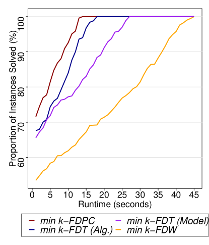
(a)

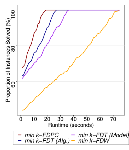
(b)

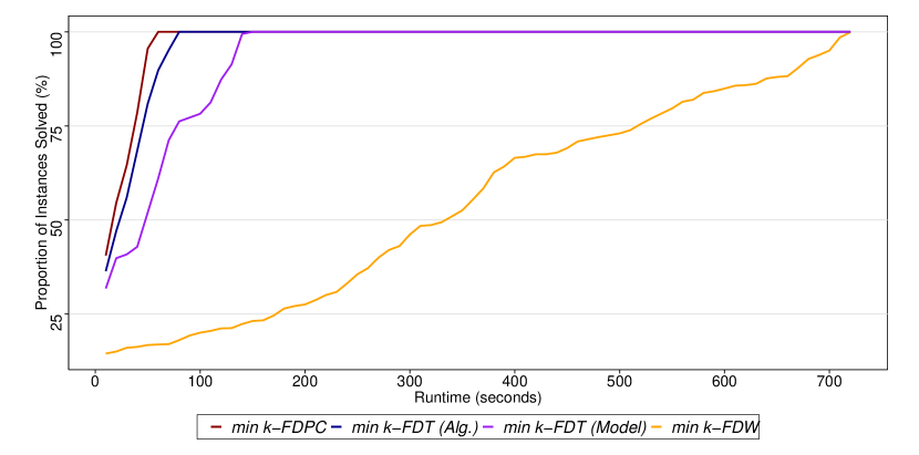
(c)

Figure 7: The percentage of all instances (y-axis) individually solvable within a certain number of seconds (x-axis).

We also evaluate how the models scale in terms of complexity of the instances of each dataset. We focus on the size $k$ of the flow decomposition since the models have size linear in $k$. In Table 1 we group the graphs into ranges based on the minimum size of a flow decomposition into paths or cycles since this is the most basic problem variant (column $min~{}k$). Since $|V|$ and $|E|$ also increase as $min~{}k$ increases, this table also indicates how the models scale in terms of graph sizes. The runtimes of all models do scale up adequately, reiterating that they are a viable candidate for real applications. The reachability model for trails (where its main decision variables $x_{uvi}$ are binary) scales better than for walks (where these variables are integer).

Table 1: Averages and standard deviations (in parentheses) for graph size, running times of the four variants of problem, and the number of iterations of Algorithm 1 until a feasible solution is found. For Algorithm 1 the runtime is the total over all iterations. If an instance did not admit a decomposition into trails, we do not include it in the runtime average for min $k$-FDT.

					min $k$-FDPC (sec)	min $k$-FDT (sec)			min $k$-FDW (sec)
	min $k$	$\#$instances	$|V|$	$|E|$		Algorithm 1	$\#$iter	Model 28
SRR020730 Salmon Adapted
	4-10	5131	23.42 (4.21)	45.12 (8.22)	3.22 (0.36)	5.13 (0.52)	2.32	10.2 (1.41)	13.42 (1.12)
	11-15	595	32.34 (3.42)	60.21 (5.41)	4.43 (0.93)	9.13 (1.23)	2.94	14.5 (1.54)	19.88 (3.41)
	16-20	236	43.81 (4.67)	71.14 (9.57)	8.68 (1.72)	14.03 (2.12)	3.20	17.2 (2.72)	28.61 (5.74)
	21-max	60	51.42 (5.23)	102.14 (11.31)	12.42 (2.41)	18.12 (3.34)	4.51	27.2 (4.41)	39.79 (5.81)
Transportation Data
	4-10	200	43.22 (6.21)	78.21 (10.13)	4.51 (0.56)	8.32 (1.13)	2.41	16.54 (2.12)	28.22 (3.31)
	11-15	150	50.74 (7.51)	83.21 (7.65)	7.13 (1.32)	15.21 (2.41)	3.52	21.33 (3.23)	53.15 (6.13)
	16-20	50	64.33 (4.78)	93.21 (5.11)	10.42 (2.13)	17.89 (3.29)	5.93	28.92 (4.09)	78.61 (7.21)
	21-max	20	80.32 (5.21)	130.1 (3.13)	14.54 (1.21)	24.72 (2.12)	6.32	36.94 (3.21)	112.71 (6.88)
E. coli Strains	4-10	80	48.21 (5.41)	82.13 (7.24)	8.51 (2.41)	14.13 (3.13)	4.33	22.41 (5.31)	56.12 (18.25)
	11-15	50	63.73 (11.42)	90.22 (12.31)	9.24 (3.13)	17.31 (4.41)	5.92	35.38 (10.24)	147.21 (27.13)
	16-20	50	78.34 (22.14)	108.01 (15.44)	17.23 (4.62)	25.89 (7.13)	6.24	53.33 (14.41)	297.35 (42.34)
	21-25	50	91.41 (28.13)	140.13 (17.62)	24.46 (8.42)	30.43 (9.31)	7.51	61.42 (22.14)	412.32 (58.42)
	26-30	50	100.81 (33.32)	156.32 (24.54)	36.93 (10.13)	45.13 (13.41)	8.43	78.43 (29.43)	523.52 (58.21)
	31-max	75	120.42 (30.34)	176.42 (30.32)	60.61 (12.42)	79.41 (18.31)	10.21	144.31 (34.62)	657.64 (63.55)

Notice that the scalability in terms of $min~{}k$ was an issue for MFD algorithms on DAGs before the ILP of Dias et al., (2022) because the previous exact FPT algorithm of Kloster et al., (2018) had an exponential dependency on $min~{}k$. Our results imply that also for cyclic graphs, ILP-based solutions have no issues in scaling to larger values of $min~{}k$. Thus, even if an FPT algorithm for MFD in graphs with cycles (parameterized by the minimum size of a solution) is open, our results suggest that such an FPT algorithm might not be necessary for practice.

To compare the three problem variants, in Table 2 we study each decomposition type’s minimum size. Since a decomposition with trails does not always exist, we also show the percentage of instances admitting such a decomposition. While all instances for all three datasets always admit a decomposition into trails for $min~{}k\leq 15$, for larger $min~{}k$ values, up to 10%, 5%, and 24% of the instances in the first, second and third datasets, respectively, do not admit such a decomposition. On average, we observe that the minimum solution size for min $k$-FDPC is more significant than for min $k$-FDT, which is more prominent for min $k$-FDW. This is explained by the fact that a trail may use a node multiple times, and a walk may also use an edge numerous times. As such, a trail or a walk may combine a source-to-sink path with one or more cycles if their weights can be appropriately adjusted to form a flow decomposition. All these insights show that there is a clear difference between the problem (as also discussed in Section 1), and that all the different variants may be explored in applications.

Table 2: Average minimum solution sizes for the flow decomposition problem into path or cycles (also split into the average number of paths and cycles), into trails (and the percentage of instances admitting a flow decomposition into trails), and into walks.

. min $k$-FDPC min $k$-FDT min $k$-FDW min $k$ $\#$paths $\#$cycles $\#$path or cycles $\#$trails $\%$feasible $\#$walks SRR020730 Salmon Adapted 4-10 5.1 4.4 9.5 3.5 100 2.8 11-15 7.1 6.2 13.3 5.1 100 4.3 16-20 9.7 8.1 17.7 5.8 93 5.4 21-max 13.1 10.3 23.3 10.1 90 9.8 Transportation Data 4-10 5.4 3.2 8.6 4.4 100 3.4 11-15 6.1 4.4 10.5 5.9 100 4.8 16-20 8.2 7.3 15.5 7.3 98 5.4 21-max 10.1 8.3 18.4 8.8 95 4.8 E. coli Strains 4-10 5.3 4.9 10.2 4.5 100 3.1 11-15 8.9 4.4 13.2 8.2 100 6.8 16-20 10.5 6.3 16.8 9.1 100 7.8 21-25 15.2 8.5 23.7 12.6 90 9.9 26-30 19.3 7.1 26.4 15.1 84 12.4 31-max 23.1 11.4 34.5 20.1 76 19.6

Finally, we analyze the two solutions for min $k$-FDT, constraint generation (Model 27) and Model 28 with variables $x_{uvi}$ binary. While both are efficient, the former is generally faster than the latter because it has a smaller number of constraints, and on our data, it also requires a small number of iterations (at most 11). However, there is no guarantee that it will be concluded after a small number of iterations in general (but as mentioned in Section 3.2, it does find a feasible decomposition after a finite number of iterations). Another advantage provided by the constraint generation formulation is that algorithmic verification procedures can assist it (in the same way as we delegated the strong connectivity check to an algorithm) and use this to craft more straightforward constraints in the original model (in our case, simple constraints based on out-going edges).

5 Conclusions and Future Work

Flow decomposition is a common problem present in different fields of science, including Computer Science, Bioinformatics and Transportation. Throughout the literature, there has been considerable effort into solving this problem, especially on acyclic inputs. This is mainly because acyclicity guarantees strong properties that can be used to develop algorithms (fixed-parameter tractable, approximation). However, for graphs that contain cycles, there has yet to be an exact solution proposed so far, the few current approaches being heuristics based on greedy algorithms.

This paper considers three natural variants of the flow decomposition problem in graphs with cycles: decompositions into paths or cycles, trails, and walks, respectively. Our ILP formulations generally adopt the same strategy as in the acyclic case from Dias et al., (2022), namely formulating what constitutes an element of decomposition and then requiring that these weighted elements fit the input flow values. However, the novelty of our formulations resides in modelling the different types of walks in a cyclic graph, which is notably more involved than formulating a path in a DAG. These formulations can also be of independent interest outside the flow decomposition problem since they model basic graph-theoretic notions.

Our formulations are also extensively tested on biological and transportation datasets. Despite the problems being NP-hard, they solve any instance of the three datasets under 45 seconds, 75 seconds, and 12 minutes, respectively. Nevertheless, since these are the first exact solutions to the problem on cyclic graphs, the quest for more efficient solutions remains open.

As future work, it would be interesting to extend the models presented here to include other aspects of empirical data, such as all the flow decomposition problem variants discussed in Dias et al., (2022) for Bioinformatics applications. More specifically, in one problem variant, we are also given a set of paths (called subpath constraints) that must appear in at least one walk of the flow decomposition. The solution from Dias et al., (2022) for this variant can be easily adapted to the min $k$-FDPC problem (because edges are not repeated), but it remains open how to adapt it to trails or walks because they can repeat edges. In the inexact and imperfect flow decomposition variants from Dias et al., (2022), the weighted walks do not need to fit the input flow perfectly. However, the constraints modelling such solutions from Dias et al., (2022) immediately carry over to all our problem variants. Lastly, our reachability formulation can also handle problem variants in which the solution walks can pass through an edge at most a given number of times by just setting a bound to each $x_{uvi}$ variable.

Appendix A Full ILP formulation for $k$-Flow Decomposition into Paths or Cycles ($k$-FDPC)

$$\sum_{(u,v)\in E}x_{uvi}-\sum_{(v,w)\in E}x_{vwi}=0 \forall i\in\{1,\ldots,k\},\forall v\in V\setminus\{s,t\},$$ (26a)

$$f_{uv}=\sum_{i\in\{1,\dots,k\}}\pi_{uvi} \forall(u,v)\in E,$$ (26b)

$$\pi_{uvi}\leq f_{uv}x_{uvi} \forall(u,v)\in E,\forall i\in\{1,\dots,k\},$$ (26c)

$$\pi_{uvi}\leq w_{i} \forall(u,v)\in E,\forall i\in\{1,\dots,k\},$$ (26d)

$$\pi_{uvi}\geq w_{i}-(1-x_{uvi})f_{uv} \forall(u,v)\in E,\forall i\in\{1,\dots,k\},$$ (26e)

$$d_{vi}\geq d_{ui}+1+(n-1)(x_{uvi}-1) \forall(u,v)\in E,\forall i\in\{1,\dots,k\},$$ (26f)

$$\sum_{v\in V}x_{svi}+\sum_{v\in V}c_{vi}\leq 1 \forall i\in\{1,\dots,k\},$$ (26g)

$$w_{i}\in\mathbb{Z}^{+} \forall i\in\{1,\dots,k\},$$ (26h)

$$x_{uvi}\in\{0,1\} \forall(u,v)\in E,\forall i\in\{1,\dots,k\},$$ (26i)

$$\pi_{uvi}\in\mathbb{Z}^{+}\cup\{0\} \forall(u,v)\in E,\forall i\in\{1,\dots,k\},$$ (26j)

$$c_{vi}\in\{0,1\} \forall v\in V,\forall i\in\{1,\dots,k\},$$ (26k)

$$d_{vi}\in\mathbb{Z}^{+} \forall v\in V,\forall i\in\{1,\dots,k\}.$$ (26l)

Appendix B Full ILP formulation for $k$-Flow Decomposition into Trails via Constraint Generation ($k$-FDT($\mathcal{C}$))

$$\sum_{(s,v)\in E}x_{svi}\leq 1 \forall i\in\{1,\ldots,k\},$$ (27a)

$$\sum_{(u,v)\in E}x_{uvi}-\sum_{(v,w)\in E}x_{vwi}=0 \forall i\in\{1,\ldots,k\},\forall v\in V\setminus\{s,t\}$$ (27b)

$$f_{uv}=\sum_{i\in\{1,\dots,k\}}\pi_{uvi} \forall(u,v)\in E,$$ (27c)

$$\pi_{uvi}\leq f_{uv}x_{uvi} \forall(u,v)\in E,\forall i\in\{1,\dots,k\},$$ (27d)

$$\pi_{uvi}\leq w_{i} \forall(u,v)\in E,\forall i\in\{1,\dots,k\},$$ (27e)

$$\pi_{uvi}\geq w_{i}-(1-x_{uvi})f_{uv} \forall(u,v)\in E,\forall i\in\{1,\dots,k\},$$ (27f)

$$\sum_{(u,v)\in E(C)}x_{uvi}\geq|C|-M(1-\beta_{Ci}) \forall C\in\mathcal{C},\forall i\in\{1,\dots,k\},$$ (27g)

$$\sum_{(u,v)\in E(C)}x_{uvi}-|C|+1-M\beta_{Ci}\leq 0 \forall C\in\mathcal{C},\forall i\in\{1,\dots,k\},$$ (27h)

$$\sum_{(u,v)\in\delta^{+}(C)\setminus E(C)}x_{uvi}\geq\beta_{Ci} \forall C\in\mathcal{C},\forall i\in\{1,\dots,k\}$$ (27i)

$$w_{i}\in\mathbb{Z}^{+} \forall i\in\{1,\dots,k\},$$ (27j)

$$x_{uvi}\in\{0,1\} \forall(u,v)\in E,\forall i\in\{1,\dots,k\},$$ (27k)

$$\pi_{uvi}\in\mathbb{Z}^{+}\cup\{0\} \forall(u,v)\in E,\forall i\in\{1,\dots,k\},$$ (27l)

$$\beta_{Ci}\in\{0,1\} \forall C\in\mathcal{C},\forall i\in\{1,\dots,k\}.$$ (27m)

Appendix C Full ILP formulation for $k$-Flow Decomposition into Walks ($k$-FDW): $x_{uvi}$ as binary variables

$$\sum_{(s,v)\in E}x_{svi}\leq 1 \forall i\in\{1,\ldots,k\},$$ (28a)

$$\sum_{(u,v)\in E}x_{uvi}-\sum_{(v,w)\in E}x_{vwi}=0 \forall i\in\{1,\ldots,k\},\forall v\in V\setminus\{s,t\},$$ (28b)

$$f_{uv}=\sum_{i\in\{1,\dots,k\}}\pi_{uvi} \forall(u,v)\in E,$$ (28c)

$$\pi_{uvi}\leq f_{uv}x_{uvi} \forall(u,v)\in E,\forall i\in\{1,\dots,k\},$$ (28d)

$$\pi_{uvi}\leq w_{i} \forall(u,v)\in E,\forall i\in\{1,\dots,k\},$$ (28e)

$$\pi_{uvi}\geq w_{i}-(1-x_{uvi})f_{uv} \forall(u,v)\in E,\forall i\in\{1,\dots,k\},$$ (28f)

$$\sum_{(u,v)\in E}x_{uvi}\geq d_{vi} \forall v\in V\setminus\{s\},\forall i\in\{1,\dots,k\},$$ (28g)

$$x_{uvi}\geq y_{uvi} \forall(u,v)\in E,\forall i\in\{1,\dots,k\},$$ (28h)

$$\sum_{(u,v)\in E}x_{uvi}\leq\sum_{(u,v)\in E}\phi_{uvi} \forall v\in V\setminus\{s\},\forall i\in\{1,\dots,k\},$$ (28i)

$$\sum_{(u,v)\in E}x_{uvi}\leq|E|\sum_{(u,v)\in E}y_{uvi} \forall v\in V\setminus\{s\},\forall i\in\{1,\dots,k\},$$ (28j)

$$\sum_{(u,v)\in E}y_{uvi}\leq 1 \forall v\in V\setminus\{s\},\forall i\in\{1,\dots,k\},$$ (28k)

$$d_{si}=1 \forall i\in\{1,\dots,k\},$$ (28l)

$$\phi_{uvi}\leq ny_{uvi} \forall(u,v)\in E,\forall i\in\{1,\dots,k\},$$ (28m)

$$\phi_{uvi}\geq-ny_{uvi} \forall(u,v)\in E,\forall i\in\{1,\dots,k\},$$ (28n)

$$\phi_{uvi}\leq(d_{vi}-d_{ui})+(1-y_{uvi})n \forall(u,v)\in E,\forall i\in\{1,\dots,k\},$$ (28o)

$$\phi_{uvi}\geq(d_{vi}-d_{ui})-(1-y_{uvi})n \forall(u,v)\in E,\forall i\in\{1,\dots,k\},$$ (28p)

$$w_{i}\in\mathbb{Z}^{+} \forall i\in\{1,\dots,k\},$$ (28q)

$$x_{uvi}\in\{0,1\} \forall(u,v)\in E,\forall i\in\{1,\dots,k\},$$ (28r)

$$\pi_{uvi}\in\mathbb{Z}^{+}\cup\{0\} \forall(u,v)\in E,\forall i\in\{1,\dots,k$$ (28s)

$$d_{vi}\in\mathbb{Z}^{+} \forall v\in V,\forall i\in\{1,\dots,k\},$$ (28t)

$$y_{uvi}\in\{0,1\} \forall(u,v)\in E,\forall i\in\{1,\dots,k\},$$ (28u)

$$\phi_{uvi}\in\mathbb{Z} \forall(u,v)\in E,\forall i\in\{1,\dots,k\}.$$ (28v)

Appendix D Full ILP formulation for $k$-Flow Decomposition into Walks ($k$-FDW): $x_{uvi}$ as an integer variables

$$\sum_{(s,v)\in E}x_{svi}\leq 1 \forall i\in\{1,\ldots,k\},$$ (29a)

$$\sum_{(u,v)\in E}x_{uvi}-\sum_{(v,w)\in E}x_{vwi}=0 \forall i\in\{1,\ldots,k\},\forall v\in V\setminus\{s,t\},$$ (29b)

$$w_{i}=\sum_{j\in\{0,\dots,\lfloor\log_{2}(\overline{w})\rfloor\}}2^{j}\zeta_{ij} \forall i\in\{1,\ldots,k\},$$ (29c)

$$f_{uv}=\sum_{i\in\{1,\dots,k\}}\sum_{j\in\{0,\dots,\lfloor\log_{2}(\overline{w})\rfloor\}}2^{j}\varphi_{uvij} \forall(u,v)\in E,$$ (29d)

$$\varphi_{uvij}\leq f_{uv}\zeta_{ij} \forall(u,v)\in E,\forall i\in\{1,\dots,k\},\forall j\in\{0,\dots,\lfloor\log_{2}(\overline{w})\rfloor\},$$ (29e)

$$\varphi_{uvij}\leq x_{uvi} \forall(u,v)\in E,\forall i\in\{1,\dots,k\},\forall j\in\{0,\dots,\lfloor\log_{2}(\overline{w})\rfloor\},$$ (29f)

$$\varphi_{uvij}\geq x_{uvi}-(1-\zeta_{ij})f_{uv} \forall(u,v)\in E,\forall i\in\{1,\dots,k\},\forall j\in\{0,\dots,\lfloor\log_{2}(\overline{w})\rfloor\},$$ (29g)

$$\sum_{(u,v)\in E}x_{uvi}\geq d_{vi} \forall v\in V\setminus\{s\},\forall i\in\{1,\dots,k\},$$ (29h)

$$x_{uvi}\geq y_{uvi} \forall(u,v)\in E,\forall i\in\{1,\dots,k\},$$ (29i)

$$\sum_{(u,v)\in E}x_{uvi}\leq\sum_{(u,v)\in E}\phi_{uvi} \forall v\in V\setminus\{s\},\forall i\in\{1,\dots,k\},$$ (29j)

$$\sum_{(u,v)\in E}x_{uvi}\leq|E|\sum_{(u,v)\in E}y_{uvi} \forall v\in V\setminus\{s\},\forall i\in\{1,\dots,k\},$$ (29k)

$$\sum_{(u,v)\in E}y_{uvi}\leq 1 \forall v\in V\setminus\{s\},\forall i\in\{1,\dots,k\},$$ (29l)

$$d_{si}=1 \forall i\in\{1,\dots,k\},$$ (29m)

$$\phi_{uvi}\leq ny_{uvi} \forall(u,v)\in E,\forall i\in\{1,\dots,k\},$$ (29n)

$$\phi_{uvi}\geq-ny_{uvi} \forall(u,v)\in E,\forall i\in\{1,\dots,k\},$$ (29o)

$$\phi_{uvi}\leq(d_{vi}-d_{ui})+(1-y_{uvi})n \forall(u,v)\in E,\forall i\in\{1,\dots,k\},$$ (29p)

$$\phi_{uvi}\geq(d_{vi}-d_{ui})-(1-y_{uvi})n \forall(u,v)\in E,\forall i\in\{1,\dots,k\},$$ (29q)

$$w_{i}\in\mathbb{Z}^{+} \forall i\in\{1,\dots,k\},$$ (29r)

$$x_{uvi}\in\mathbb{Z}^{+}\cup\{0\} \forall(u,v)\in E,\forall i\in\{1,\dots,k\},$$ (29s)

$$d_{vi}\in\mathbb{Z}^{+}\cup\{0\} \forall v\in V,\forall i\in\{1,\dots,k\},$$ (29t)

$$y_{uvi}\in\{0,1\} \forall(u,v)\in E,\forall i\in\{1,\dots,k\},$$ (29u)

$$\zeta_{ij}\in\{0,1\} \forall i\in\{1,\dots,k\},\forall j\in\{0,\dots,\lfloor\log_{2}(\overline{w})\rfloor\},$$ (29v)

$$\varphi_{uvij}\in\mathbb{Z}^{+}\cup\{0\} \forall(u,v)\in E,\forall i\in\{1,\dots,k\},\forall j\in\{0,\dots,\lfloor\log_{2}(\overline{w})\rfloor\},$$ (29w)

$$\phi_{uvi}\in\mathbb{Z} \forall(u,v)\in E,\forall i\in\{1,\dots,k\}.$$ (29x)

$$\overline{w}=\max_{(u,v)\in E}f_{uv}$$

References

- Ahuja et al., (1988) Ahuja, R. K., Magnanti, T. L., and Orlin, J. B. (1988). Network flows.
- Baaijens et al., (2020) Baaijens, J. A., Stougie, L., and Schönhuth, A. (2020). Strain-aware assembly of genomes from mixed samples using flow variation graphs. In International Conference on Research in Computational Molecular Biology, pages 221–222. Springer.
- Bar-Gera et al., (2021) Bar-Gera, H., Stabler, B., and Sall, E. (2021). Transportation networks for research core team. Transportation Network Test Problems. Available online: https://github.com/bstabler/TransportationNetworks (accessed on 3 July 2022).
- Bentley and Yao, (1976) Bentley, J. L. and Yao, A. C.-C. (1976). An almost optimal algorithm for unbounded searching. Information Processing Letters, 5(3):82–87.
- Cáceres et al., (2022) Cáceres, M., Cairo, M., Grigorjew, A., Khan, S., Mumey, B., Rizzi, R., Tomescu, A. I., and Williams, L. (2022). Width helps and hinders splitting flows. In ESA 2022 - European Symposium on Algorithms. To appear, https://arxiv.org/abs/2207.02136.
- Cohen et al., (2014) Cohen, R., Lewin-Eytan, L., Naor, J. S., and Raz, D. (2014). On the effect of forwarding table size on SDN network utilization. In IEEE INFOCOM 2014-IEEE conference on computer communications, pages 1734–1742. IEEE.
- Dantzig et al., (1954) Dantzig, G., Fulkerson, R., and Johnson, S. (1954). Solution of a large-scale traveling-salesman problem. Journal of the operations research society of America, 2(4):393–410.
- Dias et al., (2022) Dias, F. H. C., Williams, L., Mumey, B., and Tomescu, A. I. (2022). Fast, Flexible, and Exact Minimum Flow Decompositions via ILP. In RECOMB 2022 - 26th Annual International Conference on Research in Computational Molecular Biology, volume 13278 of Lecture Notes in Computer Science, pages 230–245. Springer.
- Grabherr et al., (2011) Grabherr, M. G., Haas, B. J., Yassour, M., Levin, J. Z., Thompson, D. A., Amit, I., Adiconis, X., Fan, L., Raychowdhury, R., Zeng, Q., et al. (2011). Trinity: reconstructing a full-length transcriptome without a genome from RNA-Seq data. Nature biotechnology, 29(7):644.
- Gurobi Optimization, LLC, (2021) Gurobi Optimization, LLC (2021). Gurobi Optimizer Reference Manual.
- Hartman et al., (2012) Hartman, T., Hassidim, A., Kaplan, H., Raz, D., and Segalov, M. (2012). How to split a flow? In 2012 Proceedings IEEE INFOCOM, pages 828–836. IEEE.
- Hong et al., (2013) Hong, C.-Y., Kandula, S., Mahajan, R., Zhang, M., Gill, V., Nanduri, M., and Wattenhofer, R. (2013). Achieving high utilization with software-driven wan. In Proceedings of the ACM SIGCOMM 2013 conference on SIGCOMM, pages 15–26.
- Kloster et al., (2018) Kloster, K., Kuinke, P., O’Brien, M. P., Reidl, F., Villaamil, F. S., Sullivan, B. D., and van der Poel, A. (2018). A practical fpt algorithm for flow decomposition and transcript assembly. In 2018 Proceedings of the Twentieth Workshop on Algorithm Engineering and Experiments (ALENEX), pages 75–86. SIAM.
- Koren, (2018) Koren, I. (2018). Computer arithmetic algorithms. AK Peters/CRC Press.
- Kovaka et al., (2019) Kovaka, S., Zimin, A. V., Pertea, G. M., Razaghi, R., Salzberg, S. L., and Pertea, M. (2019). Transcriptome assembly from long-read RNA-seq alignments with StringTie2. Genome biology, 20(1):1–13.
- Lin et al., (2012) Lin, Y.-Y., Dao, P., Hach, F., Bakhshi, M., Mo, F., Lapuk, A., Collins, C., and Sahinalp, S. C. (2012). Cliiq: Accurate comparative detection and quantification of expressed isoforms in a population. In International Workshop on Algorithms in Bioinformatics, pages 178–189. Springer.
- Miller et al., (1960) Miller, C. E., Tucker, A. W., and Zemlin, R. A. (1960). Integer programming formulation of traveling salesman problems. Journal of the ACM (JACM), 7(4):326–329.
- Mumey et al., (2015) Mumey, B., Shahmohammadi, S., McManus, K., and Yaw, S. (2015). Parity balancing path flow decomposition and routing. In 2015 IEEE Globecom Workshops (GC Wkshps), pages 1–6. IEEE.
- Ohst, (2015) Ohst, J. P. (2015). On the Construction of Optimal Paths from Flows and the Analysis of Evacuation Scenarios. PhD thesis, University of Koblenz and Landau, Germany.
- Olsen et al., (2020) Olsen, N., Kliewer, N., and Wolbeck, L. (2020). A study on flow decomposition methods for scheduling of electric buses in public transport based on aggregated time–space network models. Central European Journal of Operations Research, pages 1–37.
- Safikhani et al., (2013) Safikhani, Z., Sadeghi, M., Pezeshk, H., and Eslahchi, C. (2013). SSP: An interval integer linear programming for de novo transcriptome assembly and isoform discovery of RNA-seq reads. Genomics, 102(5-6):507–514.
- Sashittal et al., (2021) Sashittal, P., Zhang, C., Peng, J., and El-Kebir, M. (2021). Jumper enables discontinuous transcript assembly in coronaviruses. Nature Communications, 12(1):6728.
- Schulz et al., (2012) Schulz, M. H., Zerbino, D. R., Vingron, M., and Birney, E. (2012). Oases: robust de novo RNA-seq assembly across the dynamic range of expression levels. Bioinformatics, 28(8):1086–1092.
- (24) Shao, M. and Kingsford, C. (2017a). Accurate assembly of transcripts through phase-preserving graph decomposition. Nature biotechnology, 35(12):1167–1169.
- (25) Shao, M. and Kingsford, C. (2017b). Theory and a heuristic for the minimum path flow decomposition problem. IEEE/ACM transactions on computational biology and bioinformatics, 16(2):658–670.
- Soltysik and Yarnold, (2010) Soltysik, R. C. and Yarnold, P. R. (2010). Two-group multioda: Mixed-integer linear programming solution with bounded . Optimal Data Analysis, 1(1):30–37.
- Studio, (2017) Studio, I. I. C. O. (2017). Cplex users manual, version 12.7.
- Taccari, (2016) Taccari, L. (2016). Integer programming formulations for the elementary shortest path problem. European Journal of Operational Research, 252(1):122–130.
- Tarjan, (1972) Tarjan, R. (1972). Depth-first search and linear graph algorithms. SIAM journal on computing, 1(2):146–160.
- Vatinlen et al., (2008) Vatinlen, B., Chauvet, F., Chrétienne, P., and Mahey, P. (2008). Simple bounds and greedy algorithms for decomposing a flow into a minimal set of paths. European Journal of Operational Research, 185(3):1390–1401.
- Williams et al., (2019) Williams, L., Reynolds, G., and Mumey, B. (2019). RNA Transcript Assembly Using Inexact Flows. In 2019 IEEE International Conference on Bioinformatics and Biomedicine (BIBM), pages 1907–1914. IEEE.
- Williams et al., (2021) Williams, L., Tomescu, A., Mumey, B. M., et al. (2021). Flow decomposition with subpath constraints. In 21st International Workshop on Algorithms in Bioinformatics (WABI 2021). Schloss Dagstuhl-Leibniz-Zentrum für Informatik.
- Zhang et al., (2021) Zhang, Q., Shi, Q., and Shao, M. (2021). Scallop2 enables accurate assembly of multiple-end rna-seq data. bioRxiv.
- Zhao et al., (2021) Zhao, J., Feng, H., Zhu, D., and Lin, Y. (2021). Multitrans: an algorithm for path extraction through mixed integer linear programming for transcriptome assembly. IEEE/ACM Transactions on Computational Biology and Bioinformatics.