Infrared Regularization and Finite Size Dynamics of Entanglement Entropy in Schwarzschild Black Hole
Abstract
In this paper, infrared regularization of semi-infinite entangling regions and island formation for regions of finite size in the eternal Schwarzschild black hole are considered. We analyze whether the complementarity property and pure state condition of entanglement entropy can be preserved in the given approximation. We propose a special regularization that satisfies these two properties. With regard to entangling regions of finite size, we derive two fundamental types of them, which we call “mirror-symmetric” (MS) and “asymmetric” (AS). For MS regions, we discover a discontinuous evolution of the entanglement entropy of Hawking radiation due to finite lifetime of the island. The entanglement entropy of matter for semi-infinite regions in two-sided Schwarzschild black hole does not follow the Page curve. The lifetime of AS regions is bounded from above due to the phenomenon that we call “Cauchy surface breaking”. Shortly before this breaking, the island configuration becomes non-symmetric. For both types of finite regions, there is a critical size, below which the island never dominates. For regions smaller than some other critical size, the island does not emerge. Finally, we show that the island prescription does not help to solve the information paradox for certain finite regions.
I Introduction
Hawking radiation is a phenomenon which opens up the window into the world of quantum effects emerging in gravity [1, 2]. Years ago, Page showed [3, 4] that a detailed comparison of the thermodynamic entropy of black holes and the entanglement entropy of their radiation results in the observation that the latter exhibits an unlimited growth and finally exceeds the Bekenstein-Hawking entropy. This is in contradiction with the expected time dependence of the entanglement entropy visualized by the Page curve, which should start decreasing after a certain point, called the Page time. The descending part of the Page curve is difficult to interpret in a straightforward way, and recently an “island proposal” was introduced to explain the stoppage of the entanglement entropy growth [5, 6, 7]. This proposal is applicable to systems with dynamical gravitational degrees of freedom. The conjecture of modifying entanglement entropy in the presence of dynamical gravity has attracted a lot of attention in recent years [8, 9, 10, 11, 12, 13, 14, 15, 16, 17, 18, 19, 20, 21, 22, 23, 24, 25, 26, 27, 28, 29, 30, 31, 32, 33, 34, 35, 36, 37, 38, 39, 40, 41, 42, 43, 44, 45, 46, 47, 48, 49, 50, 51, 52, 53, 54, 55, 56, 57, 58, 59, 60, 61, 62, 63, 64, 65, 66, 67, 68, 69, 70, 71, 72, 73, 74, 75, 76]. Entanglement islands have been studied in the setups of two-dimensional gravity [5, 15, 14, 12, 25, 24, 29, 35, 55], boundary CFT [13, 19, 43, 49, 60, 62, 63, 64, 67, 70, 76] and moving mirror models [8, 9, 10, 11, 33, 45, 37, 52, 38, 69].
In this paper, we study the properties of entanglement entropy and islands in four-dimensional Schwarzschild black hole following the s-wave approximation, proposed in [5] and used in the context of higher-dimensional black holes in [18]. This approximation, having been applied to the fields defined on the background of a higher-dimensional Schwarzschild black hole, effectively reduces the problem to a two-dimensional one. The model [18] explains how the entanglement entropy, associated with semi-infinite regions “collecting” Hawking radiation, saturates after taking into account the contribution of the entanglement island in the outer near-horizon zone of two-sided Schwarzschild black hole. The variety of papers exploiting the s-wave approximation in different contexts have been published recently [22, 31, 35, 46, 30, 44, 36, 48, 55, 61, 53, 51, 41, 56, 72, 65, 73, 71, 68, 66].
We generalize the results of [18] by considering Hawking quanta collected in entangling regions of finite extent. This problem reveals curious features of entanglement entropy in two-sided Schwarzschild black hole. One of the motivations for studying finite regions in asymptotically flat black holes is to simulate a black hole in the spacetime with a positive cosmological constant (Schwarzschild-de Sitter black hole), in which, due to the presence of a cosmological horizon, only a spatial region of finite size is available to the observer.
It is well known [77, 78] that the entanglement entropy of a pure state is exactly zero, and if this state is bipartite then the entropies of each partition are equal. In the following, we call these properties pure state condition and complementarity, respectively. The latter is commonly used in the calculations of the entanglement entropy for semi-infinite regions [18, 22, 28, 41, 74]. In Section III, we explicitly check whether these two properties hold for two-sided Schwarzschild spacetime in such a setup, i.e.,
| (1) | |||
| (2) |
We derive a special regularization prescription that allows to preserve complementarity and pure state condition in explicit calculations in two-sided Schwarzschild black hole up to a universal constant term.
In Section IV, we study the time evolution of the entanglement entropy of Hawking radiation for two fundamental types of finite entangling regions, including their island phase.
In Section V, we discuss the information paradox in the context of finite entangling regions.
II Setup
II.1 Geometry
We start with the metric of the four-dimensional Schwarzschild black hole
| (3) |
where denotes the black hole horizon, and is the angular part of the metric. Introducing Kruskal coordinates, which for the right wedge take the form
| (4) |
with the tortoise coordinate and the surface gravity , we can rewrite the metric in the form
| (5) |
with the conformal factor given by
| (6) |
In what follows, we need a formula for the radial distance for the spherically symmetric two-dimensional part of the metric. If we consider (5) as a Weyl transformed version of the metric (neglecting the angular part) with the Weyl factor , the square of the distance can be derived as
| (7) |
where bold letters denote pairs of radial and time coordinates, e.g., . In terms of ()-coordinates, the distance reads
| (8) | ||||
We use the following notation for spacetime points in the right and left wedges of the Penrose diagram, respectively
| (9) |
Note that the imaginary part of the time coordinate of implies that this point is in the left wedge.
By the infrared limit of the point , we mean that tends to spacelike infinity in the corresponding wedge along an arbitrary spacelike curve: .
II.2 Entanglement entropy
Generally speaking, the calculation of entanglement entropy in a higher-dimensional curved spacetime is an extremely challenging problem. An important suggestion made in [18] was to consider the s-wave approximation. The fact that a static observer at spatial infinity collects predominantly lower multipoles, while the higher ones backscatter in the Schwarzschild black hole potential, reduces the initially complicated setup to a simpler two-dimensional problem of calculation the entanglement entropy of conformal matter. In this case, the following expression of the entanglement entropy for separate intervals is used
| (10) | ||||
where the distance is given by (8), and denote left and right endpoints of the corresponding intervals, and is a UV cutoff.
Few remarks are in order. First, one can implicitly assume that this formula describes the entanglement entropy of free massless Dirac fermions. For flat spacetime, this formula for Dirac fermions was obtained in [79]. Taking into account the transformation properties of entanglement entropy under Weyl transformations [6], one can assume the validity of (10) for the curved background (5) at fixed values of angular coordinates. The entanglement entropy of free massless Dirac fermions in a curved background has been considered in the context of the island proposal [15, 53, 80] and for inhomogeneous non-interacting Fermi gases [81].
Second, there are two versions of the theory of free Dirac fermions, which differ in whether the fermion number is -gauged or not. As it was shown in [82], if the number of fermions is not gauged, then there is no modular invariance in the theory, and vice versa 111We thank an anonymous referee for pointing out to this issue.. At the same time, the derivation of the formula (10) in flat spacetime [79] is based on ungauged theory. Modular transformations are “large” diffeomorphisms, and the absence of modular invariance could be an obstacle in obtaining the formula (10) for free Dirac fermions in a curved background. However, there are two special cases. For one interval, , the formula (10) coincides with the entanglement entropy of any two-dimensional CFT. For intervals, the entanglement entropy in the modular invariant theory of two-dimensional free compact boson at the self-dual radius coincides with the entanglement entropy (10) of free Dirac fermions [83]. These facts give an independent support to the formula (10) for and intervals.
II.3 Generalized entropy functional
Recently, it was shown that the expected behavior of the Page curve emerges from the island proposal [84, 7, 5, 15]. Considering the Hartle-Hawking vacuum [85], the reduced density matrix of Hawking radiation collected in is defined by tracing out the states in the complement region , which includes the black hole interior. The island mechanism prescribes that the states in some regions , called entanglement islands, are to be excluded from tracing out.
The island contribution can be taken into account via the generalized entropy functional defined as [14, 15]
| (11) |
Here denotes the boundary of the entanglement island, is Newton’s constant, and is the entanglement entropy of conformal matter. One should extremize this functional over all possible island configurations
| (12) |
and then choose the minimal one
| (13) |
III Infrared regularization of entanglement entropy
In this section, we consider different partitions of Cauchy surfaces in Schwarzschild spacetime and propose a regularization of spacelike infinities, which allows to preserve complementarity and pure state condition of entanglement entropy within the framework of the formula (10).
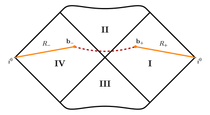
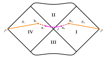
The issue can be seen from the following reasoning. Previous papers (see, for example, [18, 22, 28, 41, 74]) have extensively used the calculation of the entropy for finite complements of semi-infinite entangling regions. In particular, the entanglement entropy for the semi-infinite region , where the Hawking radiation is collected, is actually calculated in [18] using the complementarity property
| (14) |
with the complement (see Fig. 1). The calculation of leads to [18]
| (15) |
In the limit when the boundaries of the entangling regions are sent to spacelike infinities along the same timeslices (i.e., at fixed ), this formula reduces to
| (16) |
This is not what to be expected, since in this limit of the vanishingly small region , entangled particles of radiation are not collected, and the entanglement entropy (15) should have been equal to zero. However, the result grows linearly at late times. This raises a question on whether it is possible to introduce a prescription, which allows to calculate the entropy for semi-infinite entangling regions directly.
III.1 Warm-up: complementarity and pure state condition in CFT in flat background
Let us consider a finite interval on the plane with coordinates at a constant time . It is well known [86, 87] that the entanglement entropy for the subsystem is
| (17) |
Suppose that we are given a pure state on the entire line , which is a hypersurface . Pure state condition (1) requires . Sending , we obtain , so we should have had . However, the entropy as given by (17) obviously diverges as when . This simply means that the equation (17) does not hold for large . In this regard, one has to specify the size of the system, say , and then send to .
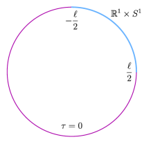
A possible way to deal with a system of a finite size is to consider a cylinder with circumference (see Fig. 2). In this case, the entanglement entropy for an interval of length is given by
| (18) |
In the limit with kept fixed, the entanglement entropy (17) for an interval on the plane is reproduced. Due to the symmetry of the expression (18), the complementarity holds automatically. Moreover, when we lengthen the interval such that the whole system is considered, i.e., (in fact, for the system on a lattice), the entanglement entropy (18) becomes
| (19) |
These simple considerations show that by introducing a suitable regularization we can preserve purity state condition and complementary property in this approximation.
An analogous closure of hypersurfaces of constant time, such that it turns into -topology, is impossible in eternal Schwarzschild black hole without violating the causal structure of this spacetime, since the left and right wedges are causally disconnected. However, we can refer to other properties of Schwarzschild spacetime. Note that there are conformal factors in the formula for entanglement entropy in a curved background, see (10) and (7). In Schwarzschild geometry, these conformal factors in Kruskal coordinates are given by (6) and tend to zero at . In addition to the fact that there are two spacelike infinities in this spacetime, one can, in principle, argue that it is possible to obtain a finite distance between spacelike infinities in the left and right wedges after mutual cancellation of IR divergences without imposing periodic boundary conditions. In what follows, we will show that we can explicitly preserve complementarity and pure state condition of entanglement entropy with its approximate expression for multiple intervals in eternal Schwarzschild black hole with one (two) endpoints(s) going to spacelike infinity in a special way, rather than cut off semi-infinite intervals.
III.2 Infrared regularization of Cauchy surfaces
Let us introduce an IR regularization of a Cauchy surface which extends between spacelike infinities in the left and right wedges of Schwarzschild (see Penrose diagram on Fig. 3). Since the Hartle–Hawking state given on is pure, we should have for the entanglement entropy. To regularize , we take a finite spacelike interval such that with the following coordinates of the IR regulators
| (20) |
Then, the entanglement entropy of conformal matter on the regularized Cauchy surface is given by
| (21) | ||||
which is, in general, divergent in the IR limit . However, this limit exists along the curves of the following type
| (22) |
where and are arbitrary constants fixed for a particular curve, and
| (23) |
Taking into account that as , the IR limit of (21) along some curve (22) is given by
| (24) |
where
| (25) |
Since this function is non-negative, the entanglement entropy can take any positive value by varying the constants , . For the same reason, we cannot get rid of the first term on the RHS of (24) by an appropriate choice of the constants , . The best we can get is to let , which according to (22) leads to
| (26) |
This means that the IR limit is taken to be asymptotically radially symmetric, and the regulators, as they go to spacelike infinity, asymptotically approach the same timeslice. For this case, the entropy of the Hartle-Hawking state defined on is given by
| (27) |
Since the entropy of a pure state should be zero, we claim that this anomalous term is to be subtracted from final answers.
At first sight, it might seem surprising that the result in the IR limit (27) depends on the UV cutoff . In fact, this is to be expected, since is the only dimensional constant, in addition to , to make the whole answer dimensionless.
The reasons why we get the entanglement entropy for infinite intervals that is not infrared divergent are the special behavior of the Weyl factor (6) at infinity, and the mutual asymptotic cancellation of the regulators. The presence of two regulators of the same sign, which cancel each other in final results, is the hallmark of two-sidedness and higher dimensionality222In fact, there are two different static patches in two-sided Schwarzschild — in the left and right wedges, respectively. Spacelike infinities are positive due to the positiveness of the radial coordinate , which can be introduced for spacetimes of higher dimensionality. For example, this is not applicable for two-dimensional Minkowski spacetime, in which spatial coordinate . Therefore, there are two spacelike infinities of different signs: . This leads to the IR divergent entanglement entropy for the Cauchy surface: as . of the eternal Schwarzschild black hole geometry, and cannot be seen as a general method of regularization of infinities during the calculation of entanglement entropy for infinite regions.
III.3 Infrared regularization of semi-infinite complement of finite entangling regions
A Cauchy surface can be divided into any number of finite entangling regions. A single finite region can lie entirely in one wedge or be extended over two. Regardless, the complement includes two semi-infinite intervals in each wedge, which stretch to the corresponding spacelike infinities . Our goal is to represent the complement as the IR limit of some finite regions (see Fig. 4). One can consider this procedure as a regularization of spacelike infinities. In this way, the endpoints are defined as
| (28) | ||||
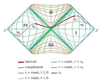
Now we want to check explicitly the complementarity property for the region and its complement . In gravitational theories, both and are determined by the island formula (13), which contains the “area term” and the matter contribution . If the island is the same both for and , to verify it suffices to compare the entanglement entropies of matter only, . Indeed, in this case, the island formulas for the region and the complement yield the same, because the same expression is extremized in (13). Therefore, further in this section, we consider only the entanglement entropy of matter .
The entanglement entropy for the region reads
| (29) |
We compare this with the entanglement entropy for the regularized complement
| (30) | ||||
The third term on the RHS tends to zero in the IR limit taken along any spacelike curve. This is because the distance to the regulator in the numerator has a counterpart in the denominator, and both have similar asymptotic behavior. The same holds for the distances to the regulator . Due to the generically divergent distance between the regulators encountered in the second term on the RHS, the IR limit of this expression exists only along the curves given by (22) and yields
| (31) |
This result does not depend on the wedge (left, right or both) in which the finite entangling region is located. The last two terms of this expression are exactly the same as we get when regularizing a Cauchy surface (24).
It is straightforward to extend this calculation to the case when consists of disjoint intervals: . In this case, the entanglement entropy for the regularized complement is given by
| (32) | ||||
The third term on the RHS, which makes the only difference with the case of a single interval, is vanishingly small in the IR limit along spacelike curves. Along the curves (22), the whole expression becomes the same as (31).
III.4 Infrared regularization consistent with complementarity and pure state condition
Let us sum up the results. We have established that in direct calculations, complementarity and pure state condition are not complied due to the anomalous term (27) and the function (25), which depends on arbitrary parameters and .
Note that the violation of pure state condition and complementarity may be related to our approach to IR regularization, the shortcomings of which we discussed for the flat case in III.1. However, due to the features of the analytically extended Schwarzschild geometry, we obtained a violation up to a constant, and not up to an IR divergent term, as in flat spacetime.
The IR limit of the entropy is well-defined along the special class of curves (22) and for any choice of the constants and . Since , we let , for which , to get rid from this contribution. This means that the regulators are to be sent to infinity asymptotically radially symmetric, and as they approach , they asymptotically fall on the same timeslice.
Then we prescribe that we should subtract the anomalous term (27). In the end, we obtain the entanglement entropy for semi-infinite regions consistent with complementarity and pure state condition.
IV Entropy dynamics for finite entangling regions
In this section, we study the dynamics of finite entangling regions affected by the presence of entanglement islands.
In the original setup [18], which describes semi-infinite entangling region , the entanglement entropy (15) enters an unbounded linear growth regime at late times
| (33) |
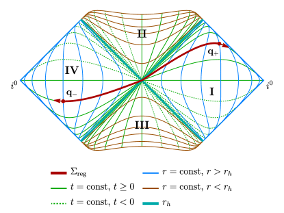
This can be interpreted as a version of the information paradox. It was shown there that taking into account the contribution of the entanglement island leads to saturation of the entanglement entropy . At late times, the island is symmetric and its endpoints are located in different wedges near the black hole horizon (see Fig. 5). The entanglement entropy in the leading-order expansion in reads
| (34) |
which is constant in time. We emphasize that this result of [18] fully relies on the complementarity property.
IV.1 Geometry and dynamics of Cauchy surfaces
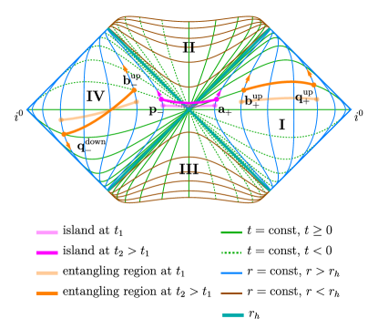
Up-down notation
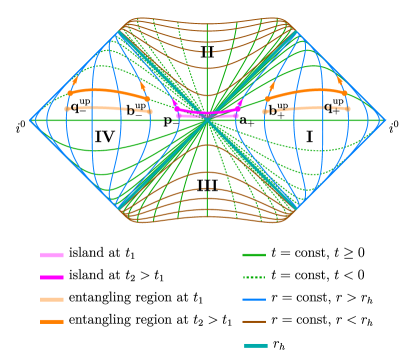
We introduce two indices for spacetime points, “up” and “down”, meaning their location with respect to the horizontal line , which stretches between spacelike infinities in the left and right wedges. This notation will prove convenient below. In the following, we use the points
| (35) | ||||
Note that points and have the same radial coordinates. Real parts of their time coordinates are opposite in sign, such a choice makes the problem time-dependent [12, 18]. Also, without loss of generality, we take radially symmetric.
Dynamics of Cauchy surfaces
Given points on the Penrose diagram, we can stretch a hypersurface to all of them as well as to the corresponding spacelike infinities . Here we develop a recipe for how to select these points so that the resulting hypersurface is a Cauchy one.
Let us divide all the points of the regularized Cauchy surface into the inner ones, whose radial coordinates are fixed and finite, and IR regulators . The latter are the endpoints of the regularized finite hypersurface, which are to be sent to .
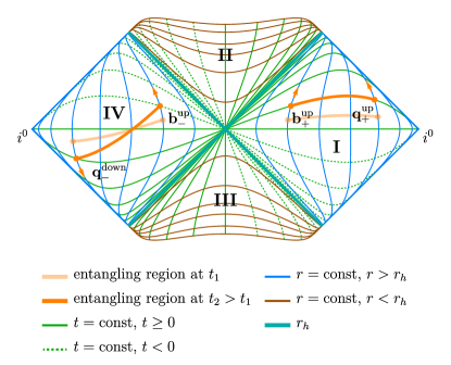
In the following, we discuss the evolution of finite regions of the type (the intermediate points and , whose radial coordinates are fixed, should not be confused with the IR regulators ). Such a choice of the region endpoints is motivated by the following reason. Moving the intermediate points along their Killing vectors in the right wedge and in the left is an isometry of the Schwarzschild spacetime. Thus, we would not get any non-trivial dynamics out of their flow. On the contrary, if we explicitly impose the relations (35), we would get the points in the right wedge moving along their Killing vectors, while in the left edge, those points with would move upwards to , and with — downwards to . This choice is not a symmetry of the problem, therefore, it would generate a non-trivial dynamics of the entropy. [12, 88]
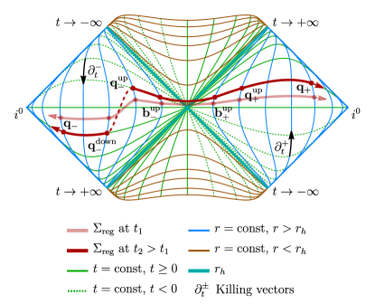
Having said this, we should emphasize that in the context of finite size regions, the choice of the points (35) has a non-trivial consequence which we call the “Cauchy surface breaking”. This phenomenon takes place when some points get separated during time evolution by a timelike interval (see Fig. 6) due to different directions of their movement on the diagram. When the Cauchy surface breaks, the problem of studying the evolution of entanglement entropy becomes ill-defined, so we should keep track of this phenomenon.
Thus, the recipe of picking a Cauchy surface is as follows:
-
a)
Since a Cauchy surface is a spacelike hypersurface, all its tangents should be spacelike. For our setup this means that if some of the inner points of a hypersurface in the left wedge lie on different sides with respect to the line , they will eventually become timelike separated. We should either avoid such hypersurfaces or consider their dynamics only for a finite time until the Cauchy surface breaks.
-
b)
Regulators are chosen according to the IR regularization described in Section III.4.
Regarding the finite regions , the Cauchy surface breaking implies:
-
c)
If the outermost inner point in the left wedge is , then the sign of its time coordinate is opposite to that of the IR regulator . This fact can naively cause the Cauchy surface breaking. However, by sending the regulator to , we effectively make the Cauchy surface breaking time infinite.
-
d)
If the outermost inner point in the left wedge is , then inevitably the corresponding Cauchy surface breaks, since the distance squared between and gets negative at some point (see Section IV.3).
If the conditions a) – c) are met, then we get a Cauchy surface, on which complementarity and pure state condition are respected. If, instead of c), the option d) takes place, we obtain a hypersurface which gets timelike at some time moment and therefore, the entanglement entropy of Hawking radiation is well-defined only for a finite time.
IV.2 Mirror-symmetric finite entangling region
Let us consider the union of two finite intervals located in the right and left wedges, whose outer boundaries are mirror-symmetric333By mirror symmetry we mean the reflection about the vertical axis of symmetry of the Penrose diagram. (see Fig. 7)
| (36) |
We call such a configuration the mirror-symmetric (MS) finite entangling region.
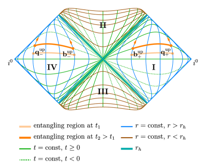
The region has a straightforward interpretation. With respect to a static observer, one can imagine each part of as a domain between two concentric spheres with radii and . Outgoing Hawking modes pass through this domain in a finite time and then escape to infinity.
The entanglement entropy of Hawking radiation collected in the MS region is given by (see Appendix (83))
| (37) | ||||
If the region is large enough, i.e., , then at intermediate times
| (38) |
the entanglement entropy of the radiation increases monotonically as
| (39) |
which is twice as fast as for the semi-infinite region (33). This behavior arises due to the fact that the distance between the points and is now time-dependent, since they lie on different timeslices. Also, provided that , this time dependence is exactly the same as that of the distance between and , which doubles the coefficient.
At late times
| (40) |
the entropy saturates at the value (see Appendix (85))
| (41) | ||||
This can be interpreted as follows. As soon as the “first”444Since the eternal black hole radiates permanently, by the “first” particle of radiation we mean the referent one emitted at . particle of the black hole radiation reaches , the entropy starts to increase, because more particles enter the domain between the spheres with radii and . As this particle reaches , the incoming and outgoing fluxes compensate each other and the entropy saturates.
Islands of finite lifetime
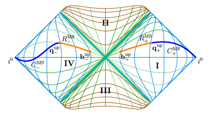
Let us consider an arbitrary island configuration , whose endpoints are parameterized as (see Fig. 9)
| (42) |
The full expression for is given in Appendix A, formula (88). Since it is symmetric under permutations of the island coordinates: , , the extremization equations for and , as well as for and , are the same. This fact tells us that we should consider a mirror-symmetric ansatz for the island
| (43) |
For intermediate times
| (44) | ||||
there is an analytical solution to the extremization equations
| (45) |
Using this, an approximate analytical expression for the entanglement entropy is given by (see Appendix (99) for details)
| (46) | ||||
The first term on the RHS is the entropy for the semi-infinite region (34) studied in [18]. Other terms represent finite size effects. Interestingly, that the third term, being vanishingly small in the large- limit, affects the dynamics, although its influence is suppressed at intermediate times. The forth term gives the anomalous term (27) in the limit .
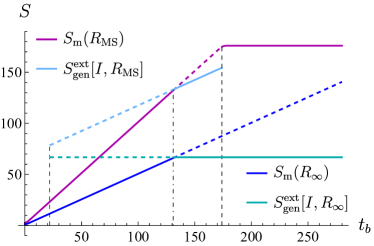
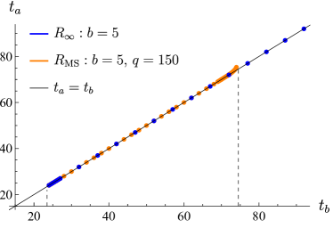
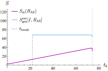
The growth of is approximately linear and is the same as of the entropy (15), unlike (39). The comparison with numerical results is shown in Fig. 10.
At late times
| (48) | ||||
along with , the generalized entropy functional grows monotonically with time (95), hence there is no solution either.
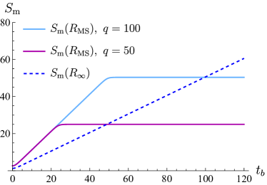
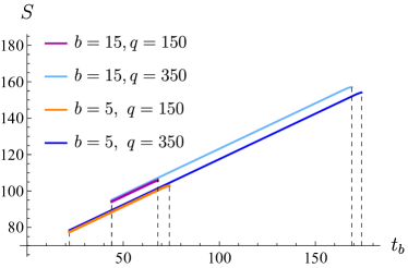
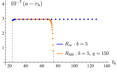
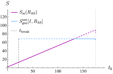
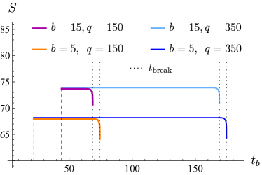
We conclude that the island exists only for a finite time, determined by the inequalities (44) (see Fig. 10). Starting from relatively small values of , the island never dominates (see Fig. 11). Reducing the size of the finite region — by increasing or decreasing — leads to a decrease in the lifetime of the island (see Fig. 12). For sufficiently large or small , the island does not appear at all, i.e., there is a region size threshold, at which the island ceases to exist.
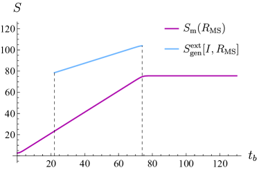
There is also a discontinuity in the entropy at the moment when the island disappears, see Fig. 10. In Section V, we will show that this behavior causes the entanglement entropy to exceed the Bekenstein-Hawking entropy.
Numerical analysis reveals several additional features. From Fig. 10 and 11, we note that the entropy for the configuration without islands reaches saturation at the moment that approximately coincides with the disappearance of the island. Also, the parameters of the island configuration and for coincides with that for , up to a short period of time before the disappearance of the island (see Fig. 13). The island gets smaller, but remains mirror-symmetric throughout the entire lifetime.
IV.3 Asymmetric finite entangling region
Cauchy surface breaking
Now let us consider the following union of two intervals, which we call the asymmetric (AS) finite entangling region (see Fig. 14)
| (49) |
Its name comes from the fact that this region is not in any sense symmetrical in the Penrose diagram.
In this setup, there is an upper bound on time (see Section IV.1): during time evolution, the point moves in time along the flow of the Killing vector , while the point moves in the opposite direction, such that the interval between them eventually becomes timelike (see Fig. 14). Indeed, consider the distance squared between and
| (50) |
This expression gets negative at the moment
| (51) |
Hence, for , the problem becomes ill-defined, since there is no longer a Cauchy surface (i.e. a spacelike hypersurface) to define a pure quantum state. A larger size of the finite region leads to a larger . In the limit , this time also gets infinite: , and the Cauchy surface breaking never happens.
For intermediate times , the entanglement entropy for grows linearly (refer to Appendix (100) for the full expression)
| (52) |
Fig. 15 shows that the entanglement entropy for almost coincides with that for the semi-infinite region , without strong dependence on . Just before the breaking time , the entropy abruptly decreases and hits the singularity, after which it is not well-defined.
Non-symmetric islands
Let us consider the island ansatz for the AS entangling region (see Fig. 16). For relatively early times, i.e.
| (53) | ||||
all the terms in the formula for the generalized entropy functional , that are non-symmetric with respect to permutations of the island coordinates: , , get suppressed (see Appendix (102)). Hence, for early times, it is reasonable to take a mirror-symmetric ansatz: , .
Then, for intermediate times
| (54) | ||||
the extremization gives the same solution as in [18]
| (55) |
The approximate analytical expression for the generalized entropy is given by (108)
| (56) | ||||
The limit at fixed of this expression recovers the semi-infinite case (34), except for the anomalous term (27), which is to be subtracted.
At late times
| (57) | ||||
the contribution of non-symmetric terms in becomes significant, which leads to the fact that the solution to the extremization equations becomes non-symmetric. This logic is verified by numerical calculations, see Fig. 17.
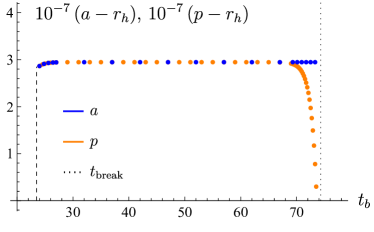
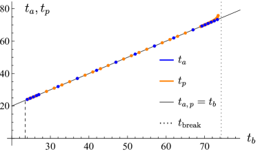
Numerical results provide us with more details. For large finite entangling regions (see Fig. 18), the dynamics of the entropy is qualitatively the same as for , except that slightly decreases just before the Cauchy surface breaking. For smaller regions, the island contribution is never dominant (see Fig. 19).
The Cauchy surface breaking, which bounds the lifetime of the configuration containing AS finite region, constrains the lifetime of the island as well. It is not the case for sufficiently large regions, such that , because in this case, there is no solution under the condition (54). However, for smaller regions, the appearance of the island may not occur before .
The lifetime of the island shortens as the size of the entangling region gets smaller (as decreases or increases, see Fig. 20).
V Information loss paradox for finite entangling regions
A Cauchy surface in the eternal Schwarzschild black hole might be divided into the semi-infinite entangling region , the region associated with the black hole , and the domain in-between. If the latter is negligible, we have
| (58) |
Given that the state is pure, the entanglement entropy obeys the complementarity property
| (59) |
The fine-grained entropy is to be bounded from above by the coarse-grained entropy
| (60) |
The latter is twice the Bekenstein-Hawking entropy [12, 18]
| (61) |
As a result, the upper bound on the entanglement entropy of Hawking radiation is expected to be [25]
| (62) |
In fact, this limit is violated due to the unstoppable growth of the entanglement entropy. This might be seen as a version of the information loss paradox [18, 12].
The evolution of the entropy changes in the presence of entanglement islands. When the island starts to dominate, the entanglement entropy is given by (34) and consists of two terms, one of which is the Bekenstein-Hawking entropy, while the other denotes additional corrections
| (63) |
These corrections are time-independent and small compared to the area term under the “black hole classicality” condition [18]
| (64) |
We say that the information paradox in two-sided Schwarzschild black hole does not arise if either the bound (62) is respected or violated only by terms suppressed under (64). Formally,
| (65) |
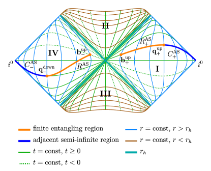
We can also divide a Cauchy surface into the region associated with the black hole , a finite entangling region , a finite domain in-between and an adjacent semi-infinite region , which extends to spacelike infinities (see Fig. 21)
| (66) |
The strong subadditivity of entanglement entropy [78] for a tripartition like (66) gives the inequality
| (67) |
Then, using the complementarity property
| (68) | ||||
and pure state condition for the total state, , we derive the upper bound on the entanglement entropy for a finite region (the strong bound)
| (69) |
We interpret its violation as the information paradox for finite entangling regions. The island prescription leads to softening of this constraint (the soft bound)
| (70) |
V.1 MS finite entangling region
Do islands for influence the bound?
As we referred to a semi-infinite outer entangling region, which is adjacent to . It can be defined as the limit of the following finite entangling region
| (71) |
The points and are IR regulators. Essentially, it is the same region as considered in [18]. Hence, we already know the features of its dynamics: the entropy for grows at early times (see (15))
| (72) |
while at late times, it saturates due to the formation of the island for this region (see (34))
| (73) |
Since the endpoints are adjacent for and , their shifts influence oppositely the formation of the islands for and for . Indeed, there are the island solutions, when the following conditions are satisfied
| : | (74) | |||
| : | ||||
We see that these conditions cannot hold together because , therefore, the corresponding islands and do not exist simultaneously.
Without islands for
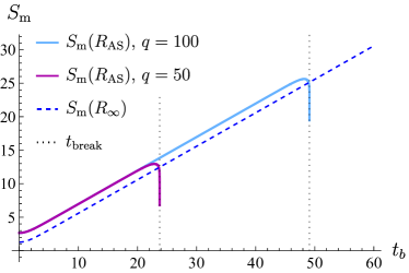
Since the entropy of matter for MS region (39) grows twice as fast as that for the semi-infinite region , and the strong bound (75) is imposed by the semi-infinite region of the same type as , the bound might be eventually violated. However, the entropy saturates at some finite value (see Section IV.2), while the bound would keep growing linearly. Therefore, if the bound is violated, then only for a finite time (see dark magenta curve in Fig. 22).
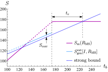
Island dominating for finite time
When the island dominates, is larger than the strong bound by , which does not change significantly if we vary . Indeed, their difference is
| (76) | ||||
with a strongly suppressed dependence on and .
After the disappearance of the island, there is a discontinuous transition to the constant entropy (41). Its value depends on and is significantly larger than the strong bound (see Fig. 22), because during the island domination, the matter entropy grows twice as fast (39) as the bound. After that, the difference decreases. The larger the value of is — the longer the constraint is violated. Thus, we say that the island prescription for does not solve the information paradox completely.
Never dominant island
For relatively small sizes of the region , the entropy of matter always dominates (see Section IV.2) and does not exceed the entropy with an island
| (77) |
hence, the soft bound is not violated.
V.2 AS finite entangling region
The semi-infinite adjacent region for AS region turns out to be neither of MS type nor AS. It can be defined as the following limit
| (78) |
The entropy of matter for this region is (see Appendix (109))
| (79) |
which is time-independent, because all points of lie on the same timeslice. This entropy is of order of , and hence, it is subdominant compared to . This means that there is no information paradox for the region even without islands.
As for the region , the strong bound (69) is explicitly given by
| (80) |
We want to check whether this inequality holds.
Without islands
If we do not take into account the islands for , the entanglement entropy for has the largest possible value just before the Cauchy surface breaking. For large enough , the entropy exceeds the strong bound (see dark magenta curve in Fig. 23). However, there is some critical value , such that for the Cauchy surface breaks before the strong bound is violated, and hence, the information paradox does not arise.
Island dominating for finite time
The island contribution to the generalized entropy starts to dominate for large enough . It exceeds the strong bound (69) (see Fig. 23), but the soft bound is still satisfied
| (81) |
where is given by the same expression as in the MS case (76) and is proportional to .
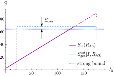
Never dominant island
If the island configuration never dominates, then the entropy of matter is always less than the generalized entropy
| (82) |
Therefore, the soft bound (70) is obeyed.
VI Conclusions and future prospects
In this paper, we address the properties of the entanglement entropy of Hawking radiation on the background of the eternal Schwarzschild black hole in the context of entangling regions of finite size. This can be seen as a starting point for studying the entropy in spacetimes with finite observable domains. Among them are de Sitter (dS) and Schwarzschild-de Sitter (SdS) universes, where a physical observer is bounded within the cosmological horizon. Therefore, only finite entangling regions are of physical significance in these spacetimes, and a generalization of the results of this paper on dS and SdS cases is needed.
We have elaborated on the infrared regularization of spacelike infinities of Cauchy surfaces and semi-infinite regions in two-sided Schwarzschild black hole. Our procedure allows to preserve complementarity and pure state condition within the approximation (10) and in the prescription of subtracting the anomalous term (27).
We have established two qualitatively different types of finite entangling regions — mirror-symmetric (MS) and asymmetric (AS). The first type represents finite domains between concentric spheres. The slope of the early-time evolution of the entanglement entropy of conformal matter for such regions is twice as large as for the canonical semi-infinite setup. For late times, the entropy saturates at a constant value even without entanglement islands. Island configurations exist only for finite time for such regions.
The outer endpoints of AS regions are chosen spatially symmetric and lie on the same timeslice. The corresponding Cauchy surfaces have a finite lifetime depending on the size of the entangling regions. In this case, the entropy grows linearly. At the time when the Cauchy surface breaks, the entanglement entropy hits singularity. Just before this moment, the island configuration becomes non-symmetric. Also, islands for the regions of both types might never dominate in the generalized entropy functional if their size is relatively small.
We have derived constraints from above on the entanglement entropy for finite entangling regions coming from strong subadditivity and complementarity. The upper bounds depend on the size of the region and on the location of its endpoints. For the AS type, the paradox is solved by entanglement islands. However, the entanglement entropy for MS regions might violate the upper bound even in the island prescription.
Acknowledgements.
Work of DA, IA and TR, which consisted in designing the project, calculating entanglement entropy and study of infrared anomalies in the context of entanglement islands (Chapters 1-3 of this paper) is supported by the Russian Science Foundation (project 20–12–00200, Steklov Mathematical Institute). DA, AB and VP are supported by the Foundation for the Advancement of Theoretical Physics and Mathematics “BASIS” (chapters 4-5). The work was performed at Steklov International Mathematical Center and supported (chapters 4-5) by the Ministry of Science and Higher Education of the Russian Federation (Agreement No. 075-15-2019-1614).Appendix A Explicit formulas for entanglement entropy for finite entangling regions
A.1 MS entangling region without island
With use of the formula for the entropy collected in multiple intervals (10) and the formula for distances (8), along with the definition of up- and down- points (35), the entanglement entropy for the mirror-symmetric finite entangling region takes the form
| (83) | ||||
At late times, such that
| (84) |
the expression simplifies to
| (85) | ||||
In the limit , we get
| (86) |
A.2 MS entangling region with island
The entropy for a non-trivial island configuration before the extremization procedure has the form (11). A general single-interval, non-symmetric ansatz for the island is . The area of its boundary is
| (87) |
With use of this, the entanglement entropy functional takes the form
| (88) | ||||
This expression is to be extremized with respect to the parameters .
The four-parameter extremization can be brought to extremization over only two parameters. Indeed, all the terms in are symmetric with respect to permutations , , hence, it is reasonable to take a mirror-symmetric ansatz for the island, . For such a choice, the full expression for the generalized entropy functional reads as
| (89) | ||||
In this expression, we can identify a part of the terms with the generalized entropy functional for the semi-infinite region and the other part with an effect of finite size of the region,
| (90) | ||||
It can be simplified further by using small-, intermediate- or large-time approximations.
We use a general property that for holds , and for and such that and holds
| (91) |
Then, for early times (small with respect to tortoise radial coordinate of the inner endpoints),
| (92) | ||||
we obtain
| (93) | ||||
Since the remaining term, describing the effect of the finite size of the region, does not depend neither on nor , there is no solution as in the semi-infinite case [18].
For late times
| (94) | ||||
the functional reduces to
| (95) | ||||
Due to linear growth, there is no solution to the extremization equation for .
For intermediate times
| (96) | ||||
where , making use of (91) and we can simplify the generalized entropy functional to
| (97) | ||||
The extremal curve with respect to time coordinate is at . Using this, we get
| (98) | ||||
We keep the vanishingly small last term from other exponential terms as that describing the leading order effect of the finite size of the region.
Taking then near-horizon-zone ansatz for the radial coordinate of the island, , , we find the analytical expression (46) for the entropy in the leading order in without solving extremization equation on explicitly,
| (99) | ||||
A.3 AS entangling region without island
The entanglement entropy for the asymmetric finite entangling region takes the form
| (100) | ||||
In the limit , we obtain
| (101) |
A.4 AS entangling region with island
The generalized entropy functional for a general non-symmetric island ansatz is
| (102) | ||||
The only non-symmetric under exchange , terms in this expression are in the last two lines. These terms are vanishingly small for times such that
| (103) | ||||
Under these assumptions taking the mirror-symmetric ansatz for island is valid. Substituting it to , we arrive at
| (104) | ||||
If we then assume that the island endpoints are near the horizon and times are long before the Cauchy surface breaking (51) (intermediate times), such that
| (105) | ||||
where , making use of (91) and we can simplify the generalized entropy functional to
| (106) | ||||
Extremizing with respect to , we obtain
| (107) | ||||
and hence an approximate analytical expression (56) in the near-horizon zone in the leading order in is
| (108) | ||||
A.5 Outer entangling region for AS finite region
The entanglement entropy for takes the form
| (109) | ||||
According to our prescription for IR regularization, the latter term is to be subtracted. Interestingly, the same result can be obtained if is considered as the complement of the regularized Cauchy surface. The entropy for it we have already calculated in (21), .
References
- Hawking [1975] S. W. Hawking, Commun. Math. Phys. 43, 199 (1975), [Erratum: Commun.Math.Phys. 46, 206 (1976)].
- Hawking [1976] S. W. Hawking, Phys. Rev. D 14, 2460 (1976).
- Page [1993] D. N. Page, Phys. Rev. Lett. 71, 3743 (1993), arXiv:hep-th/9306083 .
- Page [2013] D. N. Page, JCAP 09, 028 (2013), arXiv:1301.4995 [hep-th] .
- Penington [2020] G. Penington, JHEP 09, 002 (2020), arXiv:1905.08255 [hep-th] .
- Almheiri et al. [2019a] A. Almheiri, N. Engelhardt, D. Marolf, and H. Maxfield, JHEP 12, 063 (2019a), arXiv:1905.08762 [hep-th] .
- Almheiri et al. [2020a] A. Almheiri, R. Mahajan, J. Maldacena, and Y. Zhao, JHEP 03, 149 (2020a), arXiv:1908.10996 [hep-th] .
- Davies and Fulling [1976] P. C. W. Davies and S. A. Fulling, Proc. Roy. Soc. Lond. A 348, 393 (1976).
- Good et al. [2017] M. R. R. Good, K. Yelshibekov, and Y. C. Ong, JHEP 03, 013 (2017), arXiv:1611.00809 [gr-qc] .
- Chen and Yeom [2017] P. Chen and D.-h. Yeom, Phys. Rev. D 96, 025016 (2017), arXiv:1704.08613 [hep-th] .
- Good et al. [2020] M. R. R. Good, E. V. Linder, and F. Wilczek, Phys. Rev. D 101, 025012 (2020), arXiv:1909.01129 [gr-qc] .
- Almheiri et al. [2019b] A. Almheiri, R. Mahajan, and J. Maldacena, (2019b), arXiv:1910.11077 [hep-th] .
- Rozali et al. [2020] M. Rozali, J. Sully, M. Van Raamsdonk, C. Waddell, and D. Wakeham, JHEP 05, 004 (2020), arXiv:1910.12836 [hep-th] .
- Penington et al. [2022] G. Penington, S. H. Shenker, D. Stanford, and Z. Yang, JHEP 03, 205 (2022), arXiv:1911.11977 [hep-th] .
- Almheiri et al. [2020b] A. Almheiri, T. Hartman, J. Maldacena, E. Shaghoulian, and A. Tajdini, JHEP 05, 013 (2020b), arXiv:1911.12333 [hep-th] .
- Gautason et al. [2020] F. F. Gautason, L. Schneiderbauer, W. Sybesma, and L. Thorlacius, JHEP 05, 091 (2020), arXiv:2004.00598 [hep-th] .
- Anegawa and Iizuka [2020] T. Anegawa and N. Iizuka, JHEP 07, 036 (2020), arXiv:2004.01601 [hep-th] .
- Hashimoto et al. [2020] K. Hashimoto, N. Iizuka, and Y. Matsuo, JHEP 06, 085 (2020), arXiv:2004.05863 [hep-th] .
- Sully et al. [2021] J. Sully, M. Van Raamsdonk, and D. Wakeham, JHEP 03, 167 (2021), arXiv:2004.13088 [hep-th] .
- Hartman et al. [2020] T. Hartman, E. Shaghoulian, and A. Strominger, JHEP 07, 022 (2020), arXiv:2004.13857 [hep-th] .
- Krishnan et al. [2020] C. Krishnan, V. Patil, and J. Pereira, (2020), arXiv:2005.02993 [hep-th] .
- Alishahiha et al. [2021] M. Alishahiha, A. Faraji Astaneh, and A. Naseh, JHEP 02, 035 (2021), arXiv:2005.08715 [hep-th] .
- Geng and Karch [2020] H. Geng and A. Karch, JHEP 09, 121 (2020), arXiv:2006.02438 [hep-th] .
- Chen et al. [2020a] H. Z. Chen, R. C. Myers, D. Neuenfeld, I. A. Reyes, and J. Sandor, JHEP 10, 166 (2020a), arXiv:2006.04851 [hep-th] .
- Almheiri et al. [2021] A. Almheiri, T. Hartman, J. Maldacena, E. Shaghoulian, and A. Tajdini, Rev. Mod. Phys. 93, 035002 (2021), arXiv:2006.06872 [hep-th] .
- Dong et al. [2020] X. Dong, X.-L. Qi, Z. Shangnan, and Z. Yang, JHEP 10, 052 (2020), arXiv:2007.02987 [hep-th] .
- Balasubramanian et al. [2021a] V. Balasubramanian, A. Kar, and T. Ugajin, JHEP 02, 072 (2021a), arXiv:2008.05275 [hep-th] .
- Sybesma [2021] W. Sybesma, Class. Quant. Grav. 38, 145012 (2021), arXiv:2008.07994 [hep-th] .
- Chen et al. [2020b] H. Z. Chen, R. C. Myers, D. Neuenfeld, I. A. Reyes, and J. Sandor, JHEP 12, 025 (2020b), arXiv:2010.00018 [hep-th] .
- Ling et al. [2021] Y. Ling, Y. Liu, and Z.-Y. Xian, JHEP 03, 251 (2021), arXiv:2010.00037 [hep-th] .
- Matsuo [2021] Y. Matsuo, JHEP 07, 051 (2021), arXiv:2011.08814 [hep-th] .
- Goto et al. [2021] K. Goto, T. Hartman, and A. Tajdini, JHEP 04, 289 (2021), arXiv:2011.09043 [hep-th] .
- Akal et al. [2021a] I. Akal, Y. Kusuki, N. Shiba, T. Takayanagi, and Z. Wei, Phys. Rev. Lett. 126, 061604 (2021a), arXiv:2011.12005 [hep-th] .
- Geng et al. [2021a] H. Geng, A. Karch, C. Perez-Pardavila, S. Raju, L. Randall, M. Riojas, and S. Shashi, SciPost Phys. 10, 103 (2021a), arXiv:2012.04671 [hep-th] .
- Karananas et al. [2021] G. K. Karananas, A. Kehagias, and J. Taskas, JHEP 03, 253 (2021).
- Wang et al. [2021] X. Wang, R. Li, and J. Wang, JHEP 04, 103 (2021), arXiv:2101.06867 [hep-th] .
- Kawabata et al. [2021a] K. Kawabata, T. Nishioka, Y. Okuyama, and K. Watanabe, JHEP 05, 062 (2021a), arXiv:2102.02425 [hep-th] .
- Reyes [2021] I. A. Reyes, Phys. Rev. Lett. 127, 051602 (2021), arXiv:2103.01230 [hep-th] .
- Geng et al. [2021b] H. Geng, Y. Nomura, and H.-Y. Sun, Phys. Rev. D 103, 126004 (2021b), arXiv:2103.07477 [hep-th] .
- Bhattacharya et al. [2021a] A. Bhattacharya, A. Bhattacharyya, P. Nandy, and A. K. Patra, JHEP 05, 135 (2021a), arXiv:2103.15852 [hep-th] .
- Kim and Nam [2021] W. Kim and M. Nam, Eur. Phys. J. C 81, 869 (2021), arXiv:2103.16163 [hep-th] .
- Aalsma and Sybesma [2021] L. Aalsma and W. Sybesma, JHEP 05, 291 (2021), arXiv:2104.00006 [hep-th] .
- Geng et al. [2021c] H. Geng, S. Lüst, R. K. Mishra, and D. Wakeham, jhep 08, 003 (2021c), arXiv:2104.07039 [hep-th] .
- Lu and Lin [2022] Y. Lu and J. Lin, Eur. Phys. J. C 82, 132 (2022), arXiv:2106.07845 [hep-th] .
- Akal et al. [2021b] I. Akal, Y. Kusuki, N. Shiba, T. Takayanagi, and Z. Wei, Class. Quant. Grav. 38, 224001 (2021b), arXiv:2106.11179 [hep-th] .
- Yu and Ge [2022] M.-H. Yu and X.-H. Ge, Eur. Phys. J. C 82, 14 (2022), arXiv:2107.03031 [hep-th] .
- Geng et al. [2022a] H. Geng, A. Karch, C. Perez-Pardavila, S. Raju, L. Randall, M. Riojas, and S. Shashi, JHEP 01, 182 (2022a), arXiv:2107.03390 [hep-th] .
- Ahn et al. [2022] B. Ahn, S.-E. Bak, H.-S. Jeong, K.-Y. Kim, and Y.-W. Sun, Phys. Rev. D 105, 046012 (2022), arXiv:2107.07444 [hep-th] .
- Ageev [2022] D. S. Ageev, JHEP 03, 033 (2022), arXiv:2107.09083 [hep-th] .
- Balasubramanian et al. [2021b] V. Balasubramanian, B. Craps, M. Khramtsov, and E. Shaghoulian, JHEP 10, 048 (2021b), arXiv:2107.14746 [hep-th] .
- Cao [2022] N. H. Cao, Eur. Phys. J. C 82, 381 (2022), arXiv:2108.10144 [hep-th] .
- Fernández-Silvestre et al. [2022] D. Fernández-Silvestre, J. Foo, and M. R. R. Good, Class. Quant. Grav. 39, 055006 (2022), arXiv:2109.04147 [gr-qc] .
- Azarnia et al. [2021] S. Azarnia, R. Fareghbal, A. Naseh, and H. Zolfi, Phys. Rev. D 104, 126017 (2021), arXiv:2109.04795 [hep-th] .
- Bhattacharya et al. [2021b] A. Bhattacharya, A. Bhattacharyya, P. Nandy, and A. K. Patra, JHEP 12, 091 (2021b), arXiv:2109.07842 [hep-th] .
- Aref’eva and Volovich [2021] I. Aref’eva and I. Volovich, (2021), arXiv:2110.04233 [hep-th] .
- He et al. [2022] S. He, Y. Sun, L. Zhao, and Y.-X. Zhang, JHEP 05, 047 (2022), arXiv:2110.07598 [hep-th] .
- Ageev et al. [2019] D. S. Ageev, I. Y. Aref’eva, and A. V. Lysukhina, Teor. Mat. Fiz. 201, 424 (2019).
- Omidi [2022] F. Omidi, JHEP 04, 022 (2022), arXiv:2112.05890 [hep-th] .
- Bhattacharya et al. [2022] A. Bhattacharya, A. Bhattacharyya, P. Nandy, and A. K. Patra, Phys. Rev. D 105, 066019 (2022), arXiv:2112.06967 [hep-th] .
- Geng et al. [2022b] H. Geng, A. Karch, C. Perez-Pardavila, S. Raju, L. Randall, M. Riojas, and S. Shashi, JHEP 05, 153 (2022b), arXiv:2112.09132 [hep-th] .
- Yu et al. [2022] M.-H. Yu, C.-Y. Lu, X.-H. Ge, and S.-J. Sin, Phys. Rev. D 105, 066009 (2022), arXiv:2112.14361 [hep-th] .
- Suzuki and Takayanagi [2022] K. Suzuki and T. Takayanagi, JHEP 06, 095 (2022), arXiv:2202.08462 [hep-th] .
- Hu et al. [2022a] Q.-L. Hu, D. Li, R.-X. Miao, and Y.-Q. Zeng, JHEP 09, 037 (2022a), arXiv:2202.03304 [hep-th] .
- Hu et al. [2022b] P.-J. Hu, D. Li, and R.-X. Miao, JHEP 11, 008 (2022b), arXiv:2208.11982 [hep-th] .
- Aref’eva et al. [2022] I. Y. Aref’eva, T. A. Rusalev, and I. V. Volovich, Teor. Mat. Fiz. 212, 457 (2022), arXiv:2202.10259 [hep-th] .
- Gan et al. [2022] W.-C. Gan, D.-H. Du, and F.-W. Shu, JHEP 07, 020 (2022), arXiv:2203.06310 [hep-th] .
- Basak Kumar et al. [2022] J. Basak Kumar, D. Basu, V. Malvimat, H. Parihar, and G. Sengupta, JHEP 09, 089 (2022), arXiv:2204.06015 [hep-th] .
- Azarnia and Fareghbal [2022] S. Azarnia and R. Fareghbal, Phys. Rev. D 106, 026012 (2022), arXiv:2204.08488 [hep-th] .
- Akal et al. [2022] I. Akal, T. Kawamoto, S.-M. Ruan, T. Takayanagi, and Z. Wei, JHEP 08, 296 (2022), arXiv:2205.02663 [hep-th] .
- Afrasiar et al. [2022] M. Afrasiar, J. Kumar Basak, A. Chandra, and G. Sengupta, (2022), arXiv:2205.07903 [hep-th] .
- Anand [2022] A. Anand, (2022), arXiv:2205.13785 [hep-th] .
- Ageev and Aref’eva [2022] D. S. Ageev and I. Y. Aref’eva, Eur. Phys. J. Plus 137, 1188 (2022), arXiv:2206.04094 [hep-th] .
- Djordjević et al. [2022] S. Djordjević, A. Gočanin, D. Gočanin, and V. Radovanović, Phys. Rev. D 106, 105015 (2022), arXiv:2207.07409 [hep-th] .
- Goswami and Narayan [2022] K. Goswami and K. Narayan, JHEP 10, 031 (2022), arXiv:2207.10724 [hep-th] .
- Roy Chowdhury et al. [2022] A. Roy Chowdhury, A. Saha, and S. Gangopadhyay, Phys. Rev. D 106, 086019 (2022), arXiv:2207.13029 [hep-th] .
- Geng et al. [2022c] H. Geng, L. Randall, and E. Swanson, (2022c), arXiv:2209.02074 [hep-th] .
- Solodukhin [2011] S. N. Solodukhin, Living Rev. Rel. 14, 8 (2011), arXiv:1104.3712 [hep-th] .
- Nishioka [2018] T. Nishioka, Rev. Mod. Phys. 90, 035007 (2018), arXiv:1801.10352 [hep-th] .
- Casini et al. [2005] H. Casini, C. D. Fosco, and M. Huerta, J. Stat. Mech. 0507, P07007 (2005), arXiv:cond-mat/0505563 .
- Kawabata et al. [2021b] K. Kawabata, T. Nishioka, Y. Okuyama, and K. Watanabe, JHEP 10, 227 (2021b), arXiv:2105.08396 [hep-th] .
- Dubail et al. [2017] J. Dubail, J.-M. Stéphan, J. Viti, and P. Calabrese, SciPost Phys. 2, 002 (2017), arXiv:1606.04401 [cond-mat.str-el] .
- Headrick et al. [2013] M. Headrick, A. Lawrence, and M. Roberts, J. Stat. Mech. 1302, P02022 (2013), arXiv:1209.2428 [hep-th] .
- Calabrese et al. [2009] P. Calabrese, J. Cardy, and E. Tonni, J. Stat. Mech. 0911, P11001 (2009), arXiv:0905.2069 [hep-th] .
- Cotler et al. [2019] J. Cotler, P. Hayden, G. Penington, G. Salton, B. Swingle, and M. Walter, Phys. Rev. X 9, 031011 (2019), arXiv:1704.05839 [hep-th] .
- Hartle and Hawking [1983] J. B. Hartle and S. W. Hawking, Phys. Rev. D 28, 2960 (1983).
- Calabrese and Cardy [2004] P. Calabrese and J. L. Cardy, J. Stat. Mech. 0406, P06002 (2004), arXiv:hep-th/0405152 .
- Calabrese and Cardy [2009] P. Calabrese and J. Cardy, J. Phys. A 42, 504005 (2009), arXiv:0905.4013 [cond-mat.stat-mech] .
- Hartman and Maldacena [2013] T. Hartman and J. Maldacena, JHEP 05, 014 (2013), arXiv:1303.1080 [hep-th] .