The Penrose Inequality as a Constraint on the Low Energy Limit of Quantum Gravity

Abstract

We construct initial data violating the Anti-deSitter Penrose inequality using scalars with various potentials. Since a version of the Penrose inequality can be derived from AdS/CFT, we argue that it is a new swampland condition, ruling out holographic UV completion for theories that violate it. We produce exclusion plots on scalar couplings violating the inequality, and we find no violations for potentials from string theory. In the special case where the dominant energy condition holds, we use GR techniques to prove the AdS Penrose inequality in all dimensions, assuming spherical, planar, or hyperbolic symmetry. However, our violations show that this result cannot be generically true with only the null energy condition, and we give an analytic sufficient condition for violation of the Penrose inequality, constraining couplings of scalar potentials. Like the Breitenlohner-Freedman bound, this gives a necessary condition for the stability of AdS.

Introduction. Whether or not singularities are hidden behind event horizons is a longstanding open question in general relativity. In [1] Penrose showed that if (1) the answer to this is affirmative, and (2) collapsing matter settles down to Kerr, then the existence of certain special surfaces $\sigma$ appearing in regions of strong gravity implies a lower bound on the spacetime mass:

$$G_{N}M\geq\sqrt{\frac{\text{Area}[\sigma]}{16\pi}}.$$ (1)

A proof of this inequality, named after Penrose, would amount to evidence in favor of singularities being hidden, but the inequality has not been proven except in special cases [2, 3] (see [4] for a review).

Recently, Engelhardt and Horowitz [5] gave a holographic argument for an AdS version of the Penrose inequality (PI), assuming the AdS/CFT correspondence, but not cosmic censorship nor anything about the endpoint of gravitational collapse. This suggests that hypothetical bulk matter allowing violation of the PI in AdS is incompatible with the AdS/CFT dictionary, and that the PI can serve as a new condition detecting low energy theories that cannot be UV completed in holographic quantum gravity, meaning theories that can never arise as the low-energy limit of a holographic quantum gravity theory valid at all energy scales.

In this article we construct violations of the PI for various scalar potentials, and produce exclusion plots in coupling space, delineating regions where we know that the PI is violated. Since the PI turns out to constrain neutral scalars, we find that it is distinct from the weak gravity conjecture [6]. Next, we present numerical evidence that supersymmetry is a sufficient condition for the PI. We also present an analytical sufficient condition on scalar couplings for a theory to violate the PI. Similar to the Breitenlohner-Freedman bound [7, 8], this provides a necessary condition for the stability of AdS. Next, while our work shows that general theories respecting the null energy condition (NEC) violate the PI, we are able to prove the PI in all dimensions greater than two for any theory satisfying the dominant energy condition (DEC), assuming spherical, planar, or hyperbolic symmetry.

We emphasize that while we in this work use the PI to constrain theories in the classical limit, these constraints are intimately tied to quantum gravity in the form of the AdS/CFT correspondence, which is a nonperturbative description of string theory in AdS [9, 10, 11]. This is because Penrose’s original argument for his inequality is invalid for general low energy theories in AdS, since there exist theories violating cosmic censorship in AdS [12, 13, 14, 15]. The only known way to to argue for the truth of the PI in AdS is using the full machinery of the AdS/CFT correspondence, and then taking its classical limit. Without reference to AdS/CFT, we have no principle to exclude theories violating the PI, while if we demand that our theory arises as the classical/low-energy limit of holographic quantum gravity, the PI must hold.

The Penrose Inequality in AdS/CFT. Consider an apparent horizon $\sigma$ in an asymptotically AdS_d+1 (AAdS) spacetime with mass $M$, meaning that the expansion of the outwards null geodesic congruence fired from $\sigma$ is vanishing, while the inwards expansion is non-positive. Assuming the holographic dictionary, Ref. [5] derived that

$$\text{Area}[\sigma]\leq A_{\rm BH}(M),$$ (2)

where $A_{\rm BH}(M)$ is the area of the most entropic stationary black hole of mass $M$ in the theory. This is the AdS version of the PI that can be derived in holography, and by knowing the function $A_{\rm BH}(M)$, Eq. (2) can be rewritten to give a lower bound on the mass, similar to Eq. (1) (see Eq. (4)).

The argument of [5] relied on (1) the HRT entropy formula [16, 17, 18, 19], (2) the existence of the so-called coarse grained CFT state, whose von-Neumann entropy equals $\text{Area}[\sigma]/4G_{N}$ [20, 21], and (3) the fact that there exists a gravitational path integral for the microcanonical ensemble which has stationary black holes as saddles [22, 23]. The argument also makes the reasonable assumption that there is no spontaneous breaking of time translation symmetry in the CFT microcanonical ensemble, so that the microcanonical ensemble is dual to a stationary black hole . Finally, $\sigma$ had to satisfy two technical conditions: that it becomes a proper trapped surface when perturbed slightly inwards, and that $\sigma$ is outermost minimal, meaning that there exists a spacelike or null hypersurface bounded by $\sigma$ and the conformal boundary on which no other surface is smaller (see [20, 21] for precise conditions). In the special case where $\sigma$ is an extremal surface, the first condition is not needed.

Constraining Scalar Potentials. Working with scalar fields and spherical symmetry in the classical limit, we will see that many scalar potentials that violate the DEC violate Eq. (2) as well. DEC-violating scalars are important, since they appear in known examples of AdS/CFT dualities after dimensional reduction of compact dimensions [25, 26, 27, 28]. A generic DEC violating scalar potential will not even have a positive mass theorem (PMT) [29, 30], and in these theories the PI is automatically violated, but we will also find that theories where we are unable to construct negative mass solutions, despite extensive numerical search, will frequently violate the PI.

The theories we consider have the action

$$\int\differential^{d+1}x\sqrt{-g}\left[\frac{1}{2}R+\frac{d(d-1)}{2L^{2}}-\frac{1}{2}|\nabla\phi|^{2}-V(\phi)\right],$$ (3)

where $L$ is a length scale that sets the cosmological constant, and where $V$ is a potential satisfying $V(0)=V^{\prime}(0)=0$. To look for violations of the PI, we will construct AAdS initial data on a partial Cauchy surface $\Sigma$ bounded by $\sigma$ and the conformal boundary, such that (1) $\sigma$ is an apparent horizon satisfying all the technical conditions relevant for Eq. (2), and (2) $\Sigma$ can be embedded in a larger initial dataset on a complete hypersurface. This is sufficient to test if the PI holds for $\sigma$; the full spacetime is not needed.

What scalar potentials $V(\phi)$ should we consider in order to find violations of the PI? Ref. [31] proved an AdS₄ PI assuming spherical symmetry and the DEC. Assuming the ordinary gravitational mass $M$ [32] is finite, we prove the following generalization (conjectured to be true in [33]):

Theorem 1.

Consider an asymptotically AdS_d+1≥3 spacetime with spherical ($k=1$), planar ($k=0$), or hyperbolic symmetry ($k=-1$), satisfying the Einstein equations $G_{ab}-\frac{d(d-1)}{2L^{2}}g_{ab}=8\pi G_{N}T_{ab}$ and the DEC: $T_{ab}u^{a}v^{a}\geq 0$ for all timelike $u^{a},v^{a}$. If $\sigma$ is a symmetric outermost marginally trapped surface with respect to a connected component of the conformal boundary with mass $M$, then

$$\frac{16\pi G_{N}}{(d-1)\Omega_{k}}M\geq k\left(\frac{{\rm Area}[\sigma]}{\Omega_{k}}\right)^{\frac{d-2}{d-1}}+\frac{1}{L^{2}}\left(\frac{{\rm Area}[\sigma]}{\Omega_{k}}\right)^{\frac{d}{d-1}}.$$ (4)

Here $\Omega_{k}$ is the volume of the $(d-1)$–dimensional unit sphere, the plane, or the unit hyperbolic space (or a compactification thereof, in the latter two cases). While $\Omega_{k}$ might be infinite, the ratios $\text{Area}[\sigma]/\Omega_{k}$ and $M/\Omega_{k}$ are well defined. Furthermore, taking $k=1$ and $L\rightarrow\infty$ we get the PI for spherically symmetric asymptotically flat space in general dimensions. The mass is conventionally defined so $M=0$ for pure AdS (see [34] for a discussion definitions of mass in AdS). Let us now turn to the proof.

Proof: Consider an AAdS_d+1 spacetime with spherical, planar, or hyperbolic symmetry, and consider a null gauge with coordinates $(x^{+},x^{-},\Omega^{i})$ and metric

$$\differential s^{2}=-2e^{-f(x^{+},x^{-})}\differential x^{+}\differential x^{-}+r(x^{+},x^{-})^{2}\differential\Omega_{k}^{2},$$ (5)

where $r$ is a function of $(x^{+},x^{-})$ and where $\differential\Omega_{k}^{2}$ locally is the (unit) metric on the sphere, plane, or hyperbolic space. Define $k_{\pm}^{a}=(\partial_{x^{\pm}})^{a}\equiv(\partial_{\pm})^{a}$, which has associated null expansions $\theta_{\pm}=(d-1)r^{-1}\partial_{\pm}r$. The quantity

$$\mu(x^{+},x^{-})=r^{d}\left[\frac{k}{r^{2}}-\frac{2\theta_{+}\theta_{-}}{k_{+}\cdot k_{-}(d-1)^{2}}+\frac{1}{L^{2}}\right],$$ (6)

can be seen to reduce to the spacetime mass at $r=\infty$, up to an overall factor: $16\pi G_{N}M=(d-1)\Omega_{k}\mu|_{r=\infty}$. The null-null components of the Einstein equations (in units with $8\pi G_{N}=1$) reduce to

$$\frac{rT_{\pm\pm}}{d-1} =-\partial_{\pm}f\partial_{\pm}r-\partial_{\pm}^{2}r,$$ (7)

$$\frac{rT_{+-}}{d-1} =\partial_{+}\partial_{-}r+\frac{d^{2}-3d+2}{(d-1)r}\left[\frac{e^{-f}}{2}\left(k+\frac{r^{2}}{L^{2}}\right)+\partial_{+}r\partial_{-}r\right]$$

$$\quad+\frac{r}{L^{2}}e^{-f}$$

Proceeding similarly to Ref. [35], we compute $\partial_{\pm}\mu$ and use Eqs. (7) to eliminate $\partial_{\pm}r,\partial_{\pm}^{2}r,\partial_{+}\partial_{-}r$, yielding

$$\partial_{\pm}\mu=\frac{2e^{f}r^{d}}{(d-1)^{2}}\left(T_{+-}\theta_{\pm}-\theta_{\mp}T_{\pm\pm}\right).$$ (8)

The DEC implies that $T_{\pm\pm}\geq 0$ and $T_{+-}\geq 0$. Thus, $\pm\partial_{\pm}\mu$ is positive in an untrapped region ($\theta_{+}\geq 0,\theta_{-}\leq 0$), and so there $\mu$ is monotonically non-decreasing in an outwards spacelike direction. Evaluating $\mu$ on a marginally trapped surface that can be deformed to infinity along a untrapped spacelike path, which exists by the assumption that $\sigma$ is outermost marginally trapped, gives that $kr^{d-2}+r^{d}L^{-2}\leq\mu|_{r=\infty}$. Converting $\mu|_{r=\infty}$ to mass gives Eq. (4). $\square$

Now, the above proof applies for an apparent horizon which is outermost marginally trapped, which is not always the same as outermost minimal. However, at a moment of time-symmetry the two always coincide, since in this case we have that $\theta_{\pm}=\pm\mathcal{K}$ [36], where $\mathcal{K}$ is the mean curvature of $\sigma$ in $\Sigma$, and minimality means that $\mathcal{K}=0$. Thus, to look for violations of the PI in our setup, Theorem 1 shows that we need to consider theories violating the DEC, which for (3) means potentials that are negative somewhere.

As mentioned, DEC violating potentials arise in known AdS_d+1/CFT_d dualities after dimensional reduction, but we can also see their relevance more directly. In AdS/CFT, bulk scalar fields are dual to local scalar operators $O(x)$ in the CFT that transform with scaling dimension $\Delta$ under dilatations: $O(x)\rightarrow\lambda^{\Delta}O(\lambda x)$. It turns out that whenever $O$ is a relevant operator (i.e. $\Delta<d$), we must have that $m^{2}\equiv\partial_{\phi}^{2}V(\phi)|_{\phi=0}<0$, leading to DEC violation. This follows from the standard expression for the scaling dimension $\Delta$ of $O$ [11]: $\Delta=d/2+\sqrt{(d/2)^{2}+m^{2}L^{2}}$ . $\Delta<d$ indeed means negative $m^{2}$, which is allowed as long as the Breitenlohner-Freedman (BF) bound [7, 8] is satisfied: $m^{2}\geq m_{\rm BF}^{2}\equiv-d^{2}/(4L^{2})$.

Black Hole Uniqueness, Positive Mass, and Compact Dimensions. Before constructing initial data, a few subtleties and known results should be addressed. First, the reference black hole of mass $M$ appearing in Eq. (2) is the one that dominates the microcanonical ensemble at that mass, which is the one with the largest area [23]. Thus, if there exist black holes with larger area than AdS-Schwarzschild at a given mass, we seemingly have to construct these before claiming a violation. Black hole uniqueness is not established in AdS, so this seems like a difficult task. However, spherical symmetry allows significant simplification. In the static spherically symmetric case, Ref. [38] recently proved that the NEC implies $A_{\rm BH}(M)\leq A_{\rm AdS-Schwarzschild}(M)$, so AdS-Schwarzschild is the only spherical black hole that can dominate the microcanonical ensemble. Since the theories we consider here respect the NEC, we thus know that AdS-Schwarzschild is the correct black hole to compare to in Eq. (2), assuming we can take the reference black hole to be spherically symmetric. This is reasonable, and amounts to the assumption that the CFT microcanonical ensemble on a sphere does not break rotational symmetry spontaneously (in the bulk this is the fact that introducing spin at fixed energy tends to reduce the area, as can be seen from Kerr-AdS [39] and other known spinning black hole solutions [40, 41, 42]).

Second, it has been proven that the PMT holds even in certain theories violating the DEC. The prime example is in classical supergravity (SUGRA) theories [7, 43, 8], but in Einstein-scalar theory more general results are known. It was proved in [44, 45] that the PMT holds if the scalar potential $V(\phi)$ can be written as

$$V(\phi)=\frac{d(d-1)}{2L^{2}}+(d-1)W^{\prime}(\phi)^{2}-dW(\phi)^{2}$$ (9)

for some real function $W(\phi)$ defined for all $\phi\in\mathbb{R}$ and satisfying $W^{\prime}(0)=0$ (provided we only turn on the scalar mode with fastest falloff [46, 47, 48], which is what we do here). If we considered a supersymmetric theory, $W$ would be the so-called superpotential, but supersymmetry is not required, and $W$ can be any function satisfying the above properties. Nevertheless, we keep referring to $W$ as a superpotential. It is not known whether the existence of $W$ is a necessary condition for the existence of a PMT; the proofs of [44, 45] only show that it is sufficient.

Third, suppose that an AAdS_d+1 solution is a dimensional reduction of a higher dimensional solution with some number of compact dimensions. If the higher dimensional solution is a warped product rather than a product metric between AAdS_d+1 and the compact space, then it is not a priori obvious that a violation of the lower dimensional PI implies a violation of the higher dimensional one. For theories stemming from higher dimensions, it could in principle be that the PI only is valid with all dimensions included, but our numerical findings argue against this, since potentials from known AdS/CFT dualities seem to respect the lower dimensional PI, as we will see .

Constructing Initial Data. All the quantities appearing in the Penrose inequality can be located on a single timeslice, so we can test the Penrose inequality with initial datasets rather than full spacetimes. Let us now describe how we construct initial data. A spacelike initial dataset for the Einstein-Klein-Gordon system on a manifold $\Sigma$ at a moment of time symmetry consists of a Riemannian metric $\gamma_{ab}$ and a scalar profile $\phi$ on $\Sigma$ that together satisfy the Einstein constraint equations. The extrinsic curvature $K_{ab}$ and time-derivative of $\phi$ on $\Sigma$ are both vanishing. In this case, the full constraint equations reduce to

$$\mathcal{R}+\frac{d(d-1)}{L^{2}}=|\nabla\phi|^{2}+2V(\phi),$$ (10)

where $\mathcal{R}$ is the Ricci scalar of $\gamma_{ab}$.

Next, we want the initial data to have finite mass and evolve to an AAdS spacetime, which constrains $\phi$ to fall off sufficiently fast. Furthermore, we demand $\sigma$ to be outermost minimal, so that we can test Eq. (2). Note that $K_{ab}=0$ implies that $\sigma$ is extremal, so we need not impose the condition that $\sigma$ can be perturbed inwards to a trapped surface.

To make the procedure explicit, we pick our coordinate system on $\Sigma$ to be

$$\differential s^{2} =\frac{\differential r^{2}}{1+\frac{r^{2}}{L^{2}}-\frac{\omega(r)}{r^{d-2}}}+r^{2}\differential\Omega^{2},\quad r\in[r_{0},\infty),$$ (11)

where $\omega(r)$ is a real function and $\differential\Omega^{2}$ the metric of a round unit $(d-1)$–sphere. The marginally trapped surface $\sigma$ is the sphere at $r=r_{0}>0$, and since we are considering a spacelike manifold, we need $\omega(r)\leq r^{d-2}+r^{d}L^{-2}$. As discussed in [50], the above coordinates break down only at locally stationary spheres, where the former inequality becomes an equality. Since we want $\sigma$ to be outermost minimal, one coordinate system of the form (11) must be enough to cover $\Sigma$. In these coordinates, for a general choice of scalar profile $\phi(r)$, the solution to the constraint reads (see for example [25, 50])

$$\omega(r) =e^{-h(r)}\left[\omega(r_{0})+\int_{r_{0}}^{r}\differential\rho\frac{e^{h(\rho)}\rho^{d-1}\chi(\rho)}{d-1}\right],$$ (12)

$$h(r) =\int_{r_{0}}^{r}\differential\rho\frac{\rho\phi^{\prime}(\rho)^{2}}{d-1},\ \chi(r)=\left(1+\frac{r^{2}}{L^{2}}\right)\phi^{\prime}(r)^{2}+2V\left(\phi\right).$$

To construct particular initial datasets, we must provide the profile $\phi(r)$ on $[r_{0},\infty)$, together with value for $r_{0}$. The constant $\omega(r_{0})$ is fixed by the condition of $\sigma$ being marginally trapped, giving that $\omega(r_{0})=r_{0}^{d-2}+r_{0}^{d}L^{-2}$. Finally, we can complete our initial dataset by gluing a second copy of the initial dataset to itself along $\sigma$ (possible since $\sigma$ is extremal – see [20, 21] for details).

Let us now choose concrete scalar profiles. Since we are looking for counterexamples to the PI rather than a proof, we are free to consider special initial data. We consider two types of profiles, either

$$\phi(r) =\sum_{k=0}^{3}\text{sign}(\eta_{k})\left(\frac{|\eta_{k}|}{r}\right)^{{\Delta+2k}},$$ (13)

or

$$\phi(r)=\begin{cases}\mu\log(r/R_{0})&r_{0}\leq r\leq R_{0}\\ 0&R_{0}\leq r\end{cases},$$ (14)

for general constants $\{\eta_{k}\}$ and $\{\mu,R_{0}\}$ parametrizing the initial data. After picking numerical values of $r_{0}$ and either $\{\eta_{k}\}$ or $\{\mu,R_{0}\}$, we can compute the integrals (12) numerically, and we can obtain the mass as $16\pi G_{N}M=(d-1)\text{Vol}[S^{d-1}]\omega(\infty)$. The only remaining thing to check is that $\omega(r)$ never exceeds $r^{d-2}+r^{d}L^{-2}$ for $r>r_{0}$. As long as this is true, $\sigma$ satisfies the technical conditions required for the holographic derivation of Eq. (2).

Why do we choose the profiles (13) and (14)? By trying to minimize the mass while holding $\text{Area}[\sigma]\propto r_{0}^{d-2}$ fixed, we are maximizing the chance of violating the PI, since smaller $M$ means smaller $\text{A}_{\rm BH}(M)$. To achieve a small mass, we want large regions of nonzero scalar field in order to accumulate negative energy through the potential, while minimizing the positive gradient contribution from $\chi(r)$. Thus, we want a scalar that falls off slowly and without unnecessary non-monotonic behavior. Furthermore, due to the factor $\exp[-(d-1)^{-1}\int^{\infty}_{r}\differential\rho\rho\phi^{\prime}(\rho)^{2}]$ in the integrand of Eq. (12) when computing $\omega(\infty)\propto M$, it is the behavior of $\phi$ at large $r$ that matters (or the largest values of $r$ where $\phi$ has support). Contributions to the mass from smaller $r$ are exponentially suppressed. Now, a logarithmic profile has a slow monotonic falloff, but it requires compact support in order to have the requisite asymptotics. The profile (13) has the slowest possible falloff compatible with non-compact support and standard Dirichlet boundary conditions.

We now generate a particular dataset by first drawing $r_{0}$ with a uniform distribution from the range $(10^{-2}L,20L)$, allowing both small and large black holes. For the profile (13), we draw the coefficients $\eta_{k}$ from the range $(-3r_{0},3r_{0})$, again with a uniform distribution. For the profile (14) we draw $\mu\in(0,10)$ and $R_{0}-r_{0}\in(0,100L)$. The parameter ranges are chosen partly through trial and error – if we increase the parameter ranges for $\eta_{k}$ or $\mu$, we mostly produce invalid datasets where $\omega(r)\geq r^{d-2}+r^{d}L^{2}$ at some finite $r>r_{0}$. This is not surprising, since if $\phi$ gets a large amplitude, $\omega^{\prime}(r)$ becomes large as well, causing $\omega(r)$ to overshoot $r^{d-2}+r^{d}L^{-2}$ near $r_{0}$ . Either way, the extent that our sampling of the space of profiles $\phi(r)$ is suboptimal corresponds to how much our exclusion plots below can be improved in the future.

Coupling Exclusion Plots. Let us first study $d=3$ and the potential

$$V(\phi)=-\frac{9}{16}\phi^{2}+9\phi^{3}+11\phi^{4},$$ (15)

which has $m^{2}=\frac{1}{2}m_{\rm BF}^{2}$. This theory does not have a superpotential, since solving (9) gives that a real $W(\phi)$ can only exist on a finite interval. However, we find no negative mass solutions after generating $10^{5}$ initial datasets. Nevertheless, this theory violates the PI. For example, the profile

$$\phi(r)=-\left(\frac{3.8}{r}\right)^{\Delta}\left[1+\left(\frac{3.2}{r}\right)^{2}-\left(\frac{2.4}{r}\right)^{4}\right],$$ (16)

with $r_{0}=2.5L$ yields

$$A[\sigma]/A_{\rm AdS-Schwarzschild}(M)\approx 1.2,\quad G_{N}M\approx 7L.$$ (17)

As shown by Penrose’s original argument [1], the dataset (16) cannot settle down to a stationary black hole, so it will either collapse to a naked singularity, or we will have a Coleman-DeLuccia type decay [53] , where the conformal boundary terminates in finite time, and where the event horizon grows to infinite area.

Let us now repeat the analysis for multiple potentials. In Fig. 1 we show histograms of computed ratios $\text{Area}[\sigma]/A_{\rm AdS-Schwarzschild}(M)$ in a large ensemble of initial datasets with potentials coming either from (1) dimensional reduction of SUGRA theories appearing in string theory and AdS/CFT, such as $D=11$ [27, 28], Type IIB [26], or massive Type IIA [55] SUGRA, or (2) corresponding to a free tachyonic scalars with $m^{2}>m_{\rm BF}^{2}$. In the case of SUGRA, since we use scalar theories arising from consistent truncations, our initial datasets provide valid initial datasets in the various SUGRA theories, both in the dimensional reduction and with compact dimensions included (using the embeddings in [27, 28, 26, 55]). The specific potentials are shown in the legend of Fig. 1.

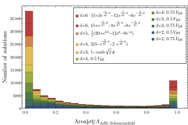
Figure 1: Plot of computed area ratios for various scalar potentials, with an ensemble of $10^{4}$ initial data sets for each potential. $V_{\rm BF}\equiv\frac{1}{2}m_{\rm BF}^{2}\phi^{2}$. For the interacting theories, the $d=6$ and $d=3$ potentials come from $S^{4}$ [27] and $S^{7}$ [28] reduction of $D=11$ SUGRA. The $d=5$ potential comes from $S^{4}$ reduction of massive Type IIA SUGRA [55], and the $d=4$ potential from $S^{5}$ reduction of Type IIB SUGRA [26].

We see that the PI holds for all our initial datasets. This does not amount to a proof that the PI holds, but it provides evidence, since for other potentials we will easily be able to produce violations while sampling from the same space of scalar profiles. This is an important consistency check on our proposal, since if the PI was violated for theories known to have a CFT dual, it presumably cannot serve as a constraint on low energy theories that can arise as the low energy limit of quantum gravity (a so-called swampland condition [56, 6, 57]) .

Consider now $d=3$ and a potential with $m^{2}=\frac{1}{2}m_{\rm BF}^{2}$, and with varying cubic and quartic couplings $g_{3},g_{4}$ (see caption of Fig. 2). Take $g_{3}\geq 0$ without loss of generality. For a given value of $g_{3}$, we can gradually lower $g_{4}$ until we find a dataset violating the PI or the PMT. In Fig. 2 we plot the highest value for $g_{4}$ for which we are able to find at least one violating dataset. Furthermore, we plot the region in $(g_{3},g_{4})$ space in which a superpotential exists. The region of coupling space below the orange (blue) markers is ruled out by the PI (PMT). For $g_{3}>0$, the PI is a stronger condition than the PMT – at least in the space of initial data we are sampling. For reasons we do not understand, at $g_{3}=0$ where $\mathbb{Z}_{2}$ symmetry is restored, the PI and PMT are violated at the same time. However, $\mathbb{Z}_{2}$ symmetry does not appear to always guarantee coincidence, as shown in Fig. 3. Nevertheless, for $d=3$ and a potential $V=\frac{1}{2}m^{2}\phi^{2}+g_{4}\phi^{4}$, we find that the PI and PMT exclusion lines do coincide as we vary $(m^{2},g_{4})$, and furthermore that exclusion line is well described by the analytical condition given below.

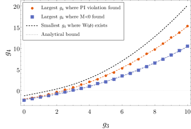
Figure 2: Exclusion plot on couplings for the potential $V(\phi)=\frac{1}{4}m_{\rm BF}^{2}\phi^{2}+g_{3}\phi^{3}+g_{4}\phi^{4}$ in $d+1=4$. Couplings below the circular markers are ruled out by the PI, while couplings below the squares are ruled out by positive mass. Blue and orange lines are quadratic fits, and couplings above the black dashed line give potentials which has superpotentials. Above the blue and orange markers, we have found no violations after the construction of $10^{5}$ initial data sets using our sampling procedure. The dotted gray line, here coinciding with the blue, shows the exclusion boundary from the analytical condition (18).

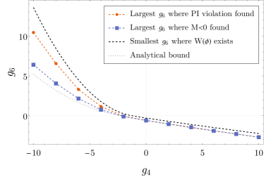
Figure 3: Exclusion plot on couplings for the potential $V(\phi)=\frac{1}{4}m_{\rm BF}^{2}\phi^{2}+g_{4}\phi^{4}+g_{6}\phi^{6}$ in $d+1=4$. The same description as in Fig. 2 applies, except the orange and blue lines are interpolations rather than fits.

Note that there are no immediately obvious changes in the potential as we cross the line into territory where we violate the PI. No new extrema develop.

Analytic bounds on couplings. So far we have given numerical bounds on couplings, through violation of the PI. We can also give analytical bounds, although they are somewhat weaker, and rely on violation of the PMT (implying PI violation). Consider the scalar profile (14), and a potential $V=\sum_{n=2}^{\infty}g_{n}\phi^{n}$. It is in fact possible to solve the integrals (12) analytically in terms of gamma functions, and while the solution is somewhat involved, the leading part of $\omega(\infty)$ in the limit $R_{0}\rightarrow\infty$ is simple, yielding, up to $\mathcal{O}(R_{0}^{-2})$ corrections,

$$\frac{\lambda\omega(\infty)}{R_{0}^{d}} =\frac{\mu^{2}}{L^{2}}+2\sum_{n=2}^{\infty}n!g_{n}\left[\frac{(1-d)\mu}{d(d-1)+\mu^{2}}\right]^{n},$$ (18)

where $\lambda\equiv d(d-1)+\mu^{2}$, and with the dependence on $r_{0}$ contained in the $\mathcal{O}(R_{0}^{-2})$ terms. A sufficient condition for violation of the PMT and PI is for the RHS of (18) to be negative for some $\mu\in\mathbb{R}$. Thus, any theory where pure AdS is nonperturbatively stable must have a positive RHS of (18) for all $\mu$. We included the exclusion line obtained from Eq. (18) in Figs. 2 and 3.

Discussion. There is by now a robust trend of proposing constraints on gravity theories in order for black holes to be well behaved semiclassically [6, 59], and for these constraints to later be proven in holography [60, 61, 62]. While the PI can be derived in holography, we have shown that it is generally false in GR, and argued that it serves as a new swampland [56, 6, 57] condition. As an example, we showed that it can be used to constrain scalar potentials for theories in AdS. If holography makes sense in asymptotically flat space, it is possible that the same logic can be applied there.