Scan-based immersed isogeometric flow analysis

Abstract

This chapter reviews the work conducted by our team on scan-based immersed isogeometric analysis for flow problems. To leverage the advantageous properties of isogeometric analysis on complex scan-based domains, various innovations have been made: (i) A spline-based segmentation strategy has been developed to extract a geometry suitable for immersed analysis directly from scan data; (ii) A stabilized equal-order velocity-pressure formulation for the Stokes problem has been proposed to attain stable results on immersed domains; (iii) An adaptive integration quadrature procedure has been developed to improve computational efficiency; (iv) A mesh refinement strategy has been developed to capture small features at a priori unknown locations, without drastically increasing the computational cost of the scan-based analysis workflow. We review the key ideas behind each of these innovations, and illustrate these using a selection of simulation results from our work. A patient-specific scan-based analysis case is reproduced to illustrate how these innovations enable the simulation of flow problems on complex scan data.

1 Introduction

The rapid developments in the field of scientific computing have opened the doors to performing computational analyses on data obtained using advanced scanning technologies (e.g., tomography or photogrammetry). Such analyses are of particular interest in applications pertaining to non-engineered systems, which are common in, for example, biomechanics, geomechanics and material science. For scan-based simulations, the data sets from which the geometric models are constructed are typically very large, and the obtained models can be very complex in terms of both geometry and topology (see Fig. 1). In the context of standard finite element analyses (FEA), scan-based simulations require image segmentation and meshing techniques to produce high-quality analysis-suitable meshes that fit to the boundaries of the domain of interest. The construction of a FEA-suitable computational domain can be an error-prone and laborious process, involving manual geometry clean-up and mesh repairing and optimization operations. Such operations can account for the majority of the total computational analysis time and form a bottleneck in the automation of scan-based simulation workflows zhang_challenges_2013 (1).

The challenges associated with the simulation workflow for complex problems sparked the development of the isogeometric analysis (IGA) paradigm by Hughes and co-workers in 2005 hughes_isogeometric_2005 (2). The pivotal idea of IGA is to directly employ the geometry interpolation functions used in computer-aided design (e.g., B-splines and NURBS rogers_introduction_2001 (3)) for the discretization of boundary value problems, thereby circumventing the problems associated with meshing. Besides the advantage of avoiding the meshing procedure and eliminating mesh-approximation errors, the use of higher-order continuous splines for the approximation of the solution has been demonstrated to yield accurate results using relatively few degrees of freedom for many (smooth) problems (see Ref. cottrell_isogeometric_2009 (4) for an overview). While isogeometric analysis has been successfully applied to complex three-dimensional problems based on (multi-patch) CAD objects (see, e.g., Refs. cottrell_isogeometric_2006 (5, 6, 7, 8, 9, 10)), its application to scan-based simulations is hindered by the absence of analysis-suitable spline-based geometry models. Although spline preprocessors have been developed over the years for a range of applications zhang_solid_2012 (11, 12, 13), the robust generation of analysis-suitable boundary-fitting volumetric splines for scan-based analyses is beyond the scope of the current tools on account of the geometrical and topological complexity typically inherent to scan data.

To still leverage the advantageous approximation properties of splines in scan-based simulations, IGA is often used in combination with immersed methods. In immersed methods, a non-boundary-fitting mesh is considered, in which the computational domain is submersed. Since the immersed domain does not align with the computational grid, some of the elements in the grid are cut by the immersed boundary and require a special treatment. The immersed approach has been considered in the finite element setting in the context of the Finite Cell Method (FCM) parvizian_finite_2007 (14, 15, 16) and CutFEM burman_ghost_2010 (17, 18, 19), amongst others. The immersed concept has also been used in combination with IGA rank_geometric_2012 (20, 21, 22), a strategy which is sometimes referred to as immersogeometric analysis kamensky_immersogeometric_2015 (23, 24). The versatility of immersed isogeometric analysis techniques with respect to the geometry representation – in the sense that the analysis procedure is not strongly affected by the complexity of the physical domain – makes it particularly attractive in the scan-based analysis setting. Applications can nowadays be found in, for example, the modeling of trabecular bone verhoosel_image-based_2015 (25, 26, 27), porous media hoang_skeleton-stabilized_2019 (28), coated metal foams duster_numerical_2012 (29), metal castings jomo_robust_2019 (30) and additive manufacturing carraturo_modeling_2020 (31).

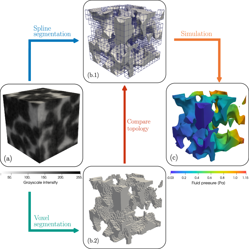
Figure 1: Illustration of the developed scan-based simulation workflow, considering a sintered glass specimen hoang_skeleton-stabilized_2019 (28) as a typical example. The grayscale scan data is shown in panel (a). A smooth reconstruction of the geometry (representing the void space) based on a spline segmentation is shown in panel (b.1), along with the computational mesh in which the geometry is submersed. The directly segmented voxel image, which is used to assess the topological correctness of the spline segmentation, is shown in panel (b.2). A typical immersed isogeometric analysis result is shown in panel (c).

Over the past decade our team has developed an analysis workflow using the immersed isogeometric analysis paradigm. This workflow is illustrated in Fig. 1. In this chapter we review the key research contributions that made this analysis workflow applicable to scan-based flow simulations:

• A spline-based geometry segmentation technique was proposed in Verhoosel et al. verhoosel_image-based_2015 (25), with further improvements being made by Divi et al. divi_error-estimate-based_2020 (32, 33). The pivotal idea of the developed segmentation strategy is that the original scan data, which is usually non-smooth (i.e., a voxel representation), is smoothed using a spline approximation. A segmentation procedure able to provide an accurate explicit parametrization of the smoothed geometry then provides a geometric description of the scan object which is suitable for immersed isogeometric analysis.

• A stabilized immersed isogeometric analysis formulation for flow problems was proposed by Hoang et al. hoang_skeleton-stabilized_2019 (28). The key idea of the proposed formulation is to use face-based stabilization techniques to make immersed simulations robust with respect to (unfavorably) cut elements, preventing the occurrence of oscillations in the velocity and pressure approximations. The stabilization terms also enable the consideration of equal-order discretizations of the velocity and pressure fields, which would otherwise cause inf-sup stability problems even in boundary-fitting finite elements hoang_mixed_2017 (34).

• An adaptive integration procedure was developed by Divi et al. divi_error-estimate-based_2020 (32) to reduce the computational cost involved in the evaluation of integrals over cut elements, thereby improving the computational efficiency of the immersed analysis workflow. Based on Strang’s lemma strang_analysis_2008 (35), an estimator for the integration error is derived, which is then used to optimally distribute integration quadrature points over cut elements.

• An error-estimation-based adaptive refinement procedure has been developed by Divi et al. divi_residual-based_2022 (36) to capture small features without drastically increasing the computational cost of the scan-based workflow. Residual-based error estimators are constructed to perform local basis function refinements to increase the resolution of the spline basis in regions where this is particularly beneficial from an accuracy point of view, without prior knowledge of the locations of these regions.

Our scan-based immersed isogeometric analysis workflow has been applied to a range of real world data problems, mainly in the context of $\mu$CT-scans. In this chapter we illustrate the capabilities of our workflow in the context of patient-specific arterial flow problems. The analysis of porous medium flows as presented in Ref. hoang_skeleton-stabilized_2019 (28), and illustrated in Fig. 1, forms another prominent application of our method.

This chapter is organized as follows. The essential innovations regarding each of the research contributions listed above are reviewed in Sections 2–5. A typical application of the developed workflow will then be discussed in Section 6. We will conclude this chapter in Section 7 with an assessment of our scan-based analysis workflow, discussing its capabilities and current limitations.

2 Spline-based geometry segmentation

In this section we review the spline-based image segmentation procedure that we have developed in the context of scan-based immersed isogeometric analysis verhoosel_image-based_2015 (25, 32, 33). In Section 2.1 we first discuss the spline-based level set construction to smoothen scan data. In Section 2.2 we review the algorithms used to construct an explicit parametrization of the scan domain. An example is finally shown in Section 2.3, illustrating the effectivity of the topology-preservation procedure developed in Ref. divi_topology-preserving_2022 (33).

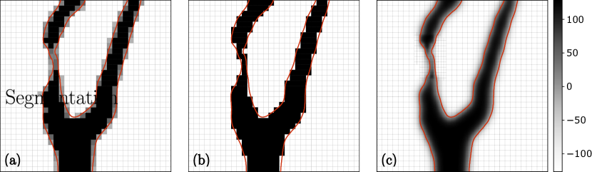
Figure 2: A two-dimensional illustration of the spline-based segmentation procedure. (a) Grayscale data on a $32\times 32$ voxel mesh, $\mathcal{T}_{\rm scan}^{\Delta}$, as in (1). (b) The voxel segmentation obtained by thresholding the grayscale data as in (2). (c) The smooth level set function obtained using a THB-spline basis constructed on the voxel mesh with local refinements as in (3). The exact immersed boundary, which is in principle unknown, is shown in red for reference.

2.1 B-spline smoothing of the scan data

The spline-based level set construction is illustrated in Fig. 2. We consider a ${d}$-dimensional scan domain, $\Omega_{\rm scan}=[0,L_{1}]\times\ldots\times[0,L_{{d}}]$ with volume $V_{\rm scan}=\prod_{i=1}^{n_{d}}L_{i}$, which is partitioned by a set of $m_{\rm vox}$ voxels, as illustrated in Fig. 2a. We denote the voxel mesh by $\mathcal{T}_{\rm scan}^{\Delta}$, with $\boldsymbol{\Delta}$ the voxel size in each direction. The grayscale intensity function is then defined as

$$g:\mathcal{T}_{\rm scan}^{\Delta}\rightarrow\mathscr{G},$$ (1)

with $\mathscr{G}$ the range of the grayscale data (e.g., from 0 to 255 for 8 bit unsigned integers). An approximation of the object $\Omega$ can be obtained by thresholding the grayscale data,

$$\Omega\approx\{\boldsymbol{x}\in\Omega_{\rm scan}|g(\boldsymbol{x})>g_{\rm crit}\}\subset\Omega_{\rm scan},$$ (2)

where $g_{\rm crit}$ is the threshold value. As a consequence of the piecewise definition of the grayscale data in equation (1), the boundary of the segmented object is non-smooth when the grayscale data is segmented directly. In the context of analysis, the non-smoothness of the boundary can be problematic, as irregularities in the surface may lead to non-physical features in the solution to the problem.

The spline-based segmentation procedure developed in Refs. verhoosel_image-based_2015 (25, 32, 33) enables the construction of a smooth boundary approximation based on voxel data. The key idea of this spline-based segmentation technique is to smoothen the grayscale function (1) by convoluting it using an $n$-dimensional spline basis, $\{N_{i,k}(\mathcal{T}_{\rm scan}^{h})\}_{i=1}^{n}$, defined over a mesh, $\mathcal{T}_{\rm scan}^{h}$, with element size, $\boldsymbol{h}=(h_{1},\ldots,h_{d})$ (note that the mesh size can differ from the voxel size). The order $k$ of the spline basis functions is assumed to be constant and isotropic. We consider THB-splines giannelli_thb-splines_2012 (37) for the construction of locally refined spaces. By considering full-regularity ($C^{k-1}$-continuous) splines of degree $k>1$, a smooth level set approximation of (1) is obtained by the convolution operation

$$f(\boldsymbol{x}) =\sum\limits_{i=1}^{n}N_{i,k}(\boldsymbol{x})a_{i}, a_{i} =\cfrac{\int_{\Omega_{\rm scan}}N_{i,k}(\boldsymbol{x})g(\boldsymbol{x}){\rm d}\boldsymbol{x}}{\int_{\Omega_{\rm scan}}N_{i,k}(\boldsymbol{x}){\rm d}\boldsymbol{x}},$$ (3)

where $\{a_{i}\}_{i=1}^{n}$ are the coefficients of the discrete level set function. The smoothed domain then follows by thresholding of this level set function:

$$\Omega\approx\{\boldsymbol{x}\in\Omega_{\rm scan}|f(\boldsymbol{x})>f_{\rm crit}\}\subset\Omega_{\rm scan}.$$ (4)

The spline level set function corresponding to the voxel data in Fig. 2a is illustrated in Fig. 2c for the case of a locally refined mesh $\mathcal{T}_{\rm scan}^{h}$ and second order ($k=2$) THB-splines. As can be seen, the object retrieved from the convoluted level set function more closely resembles the original geometry in Fig. 2a compared to the voxel segmentation in Fig. 2b. Also, as a consequence of the higher-order continuity of the spline basis, the boundaries of the domain are smooth, which is in closer agreement with reality.

The convolution operation (3) is computationally efficient, resulting from the fact that it is not required to solve a linear system of equations (in contrast to a (global) $L^{2}$-projection) and the restricted support of the convolution kernel. Moreover, the convolution strategy has various properties that are advantageous in the context of scan-based immersed isogeometric analysis (see Refs. verhoosel_image-based_2015 (25, 33) for details):

Conservation of the gray scale intensity

Under the condition that the spline basis, $\{N_{i,k}(\mathcal{T}_{\rm scan}^{h})\}_{i=1}^{n}$, satisfies the partition of unity property (e.g., B-splines, THB-splines), the smooth level set approximation (3) conserves the gray scale intensity of the original data in the sense that

$$\frac{1}{V_{\rm scan}}\int\limits_{\Omega_{\rm scan}}f\,{\rm d}V=\frac{1}{V_{\rm scan}}\int\limits_{\Omega_{\rm scan}}g\,{\rm d}V=\frac{1}{m_{\rm vox}}\sum_{K\in\mathcal{T}_{\rm scan}^{\Delta}}g(K).$$ (5)

This property ensures that there is a direct relation between the threshold value, $f_{\rm crit}$, for the smooth level set reconstruction (4) and that of the original data, $g_{\rm crit}$, in equation (2).

Local boundedness by the original data

On every voxel $K\in\mathcal{T}_{\rm scan}^{\Delta}$, the level set function (3) is bound by the extrema of the voxel function over the support extension bazilevs_isogeometric_2006 (38), $\widetilde{K}$, i.e.,

$$\min_{\boldsymbol{x}\in\widetilde{K}}g(\boldsymbol{x})\leq f(\boldsymbol{x})\leq\max_{\boldsymbol{x}\in\widetilde{K}}g(\boldsymbol{x}) \forall\boldsymbol{x}\in K.$$ (6)

These bounds preclude overshoots and undershoots, which indicates that no spurious oscillations are created by the smoothing procedure (contrasting the case of an $L^{2}$-projection).

Approximate Gaussian blurring

The spline-based convolution operation (3) can be written as an integral transform

$$f(\boldsymbol{x}) =\int_{\Omega_{\rm scan}}\mathcal{K}(\boldsymbol{x},\boldsymbol{y})g(\boldsymbol{y})\>{\rm d}\boldsymbol{y}, \mathcal{K}(\boldsymbol{x},\boldsymbol{y}) =\sum\limits_{i=1}^{n}\cfrac{N_{i,k}(\boldsymbol{x})N_{i,k}(\boldsymbol{y})}{\int_{\Omega_{\rm scan}}N_{i,k}(\boldsymbol{z})\>{\rm d}\boldsymbol{z}},$$ (7)

where $\mathcal{K}(\boldsymbol{x},\boldsymbol{y})$ is the kernel of the transformation.

The integral transform (7) acts as an approximate Gaussian filter deng_adaptive_1993 (39). We illustrate this behavior for the case of one-dimensional voxel data, which is smoothed using a B-spline basis defined on a uniform mesh, $\mathcal{T}_{\rm scan}^{h}$, with mesh size $h$. Following the derivation in Ref. verhoosel_image-based_2015 (25) – in which the essential step is to approximate the B-spline basis functions by rescaled Gaussians unser_asymptotic_1992 (40) – the integration kernel (7) can be approximated by

$$\mathcal{K}(x,y)\approx\kappa(x-y)=\frac{1}{\sigma\sqrt{2\pi}}\exp{\left({-\cfrac{(x-y)^{2}}{2\sigma^{2}}}\right)},$$ (8)

where the width of the smoothing kernel is given by $\sigma=h\sqrt{\frac{k+1}{6}}$. Next, we consider an object of size $\ell$, represented by the grayscale function

$$g(x) =\begin{cases}1&|x|<\ell/2\\ 0&\mbox{otherwise}\end{cases}.$$ (9)

This object and the corresponding approximate level set function (3) are illustrated in Fig. 3 for various feature-size-to-mesh ratios, $\hat{\ell}=\ell/h=2,1,\frac{1}{2}$, and B-spline degrees, $k=2,3,4$. Following the (Fourier) analysis in Ref. divi_topology-preserving_2022 (33), the value of the smoothed level set function at $x=0$ follows as

$$\hat{f}_{1}(0)=\hat{\ell}\sqrt{\frac{3}{\pi(k+1)}}~{}\exp{\left(-\frac{3\hat{\ell}^{2}}{16(k+1)}\right)},$$ (10)

which conveys that the maximum value of the smoothed level set depends linearly on the relative feature size $\hat{\ell}$ (for sufficiently small $\hat{\ell}$), and decreases with increasing B-spline order.

Fig. 3(a) shows the case for which the considered feature is twice as large as the mesh size, i.e., $\hat{\ell}=2$, illustrating that the sharp boundaries of the original grayscale function are significantly smoothed. The decrease in the maximum level set value as given by equation (10) is observed. When the level set function is segmented by a threshold of $g_{\rm crit}=0.5$, a geometric feature that closely resembles the original one is recovered. Fig. 3(b)-3(c) illustrate cases where the feature length, $\ell$, is not significantly larger than the mesh size, $h$. For the case where the feature size is equal to the size of the mesh, the maximum of the level set function drops significantly compared to the case of $\hat{\ell}=2$. When considering second-order B-splines, the maximum is still marginally above $g_{\rm crit}=0.5$. Although the recovered feature is considerably smaller than the original one, it is still detected in the segmentation procedure. When increasing the B-spline order, the maximum value of the level set drops below the segmentation threshold, however, indicating that the feature will no longer be detected. When decreasing the feature length further, as illustrated in Fig. 3(c), the feature would be lost when segmentation is performed with $g_{\rm crit}=0.5$, regardless of the order of the spline basis.

The implications of this smoothing behavior of the convolution operation (3) in the context of the spline-based segmentation will be discussed in Section 2.3.

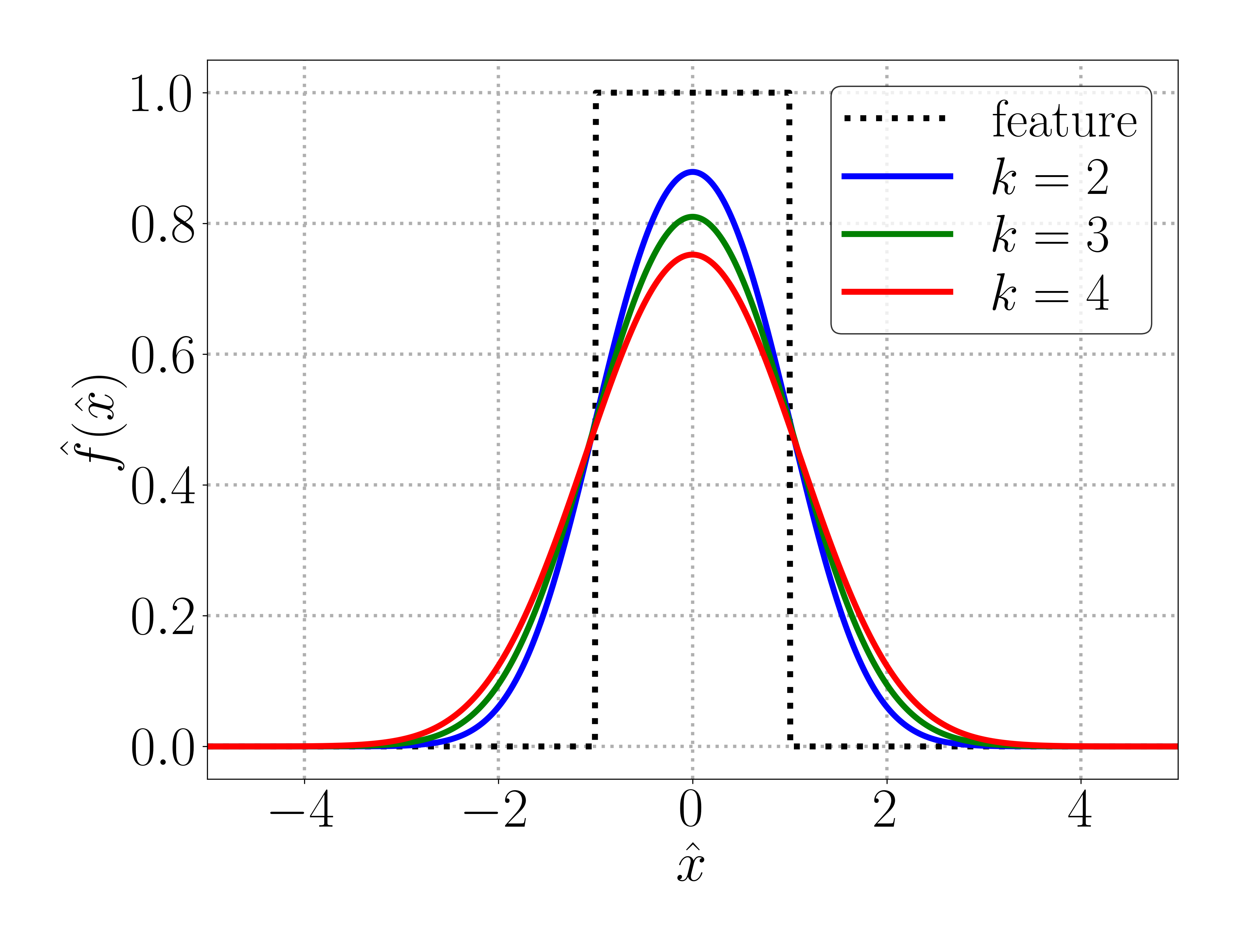
(a) $\hat{\ell}=\frac{\ell}{h}=2$

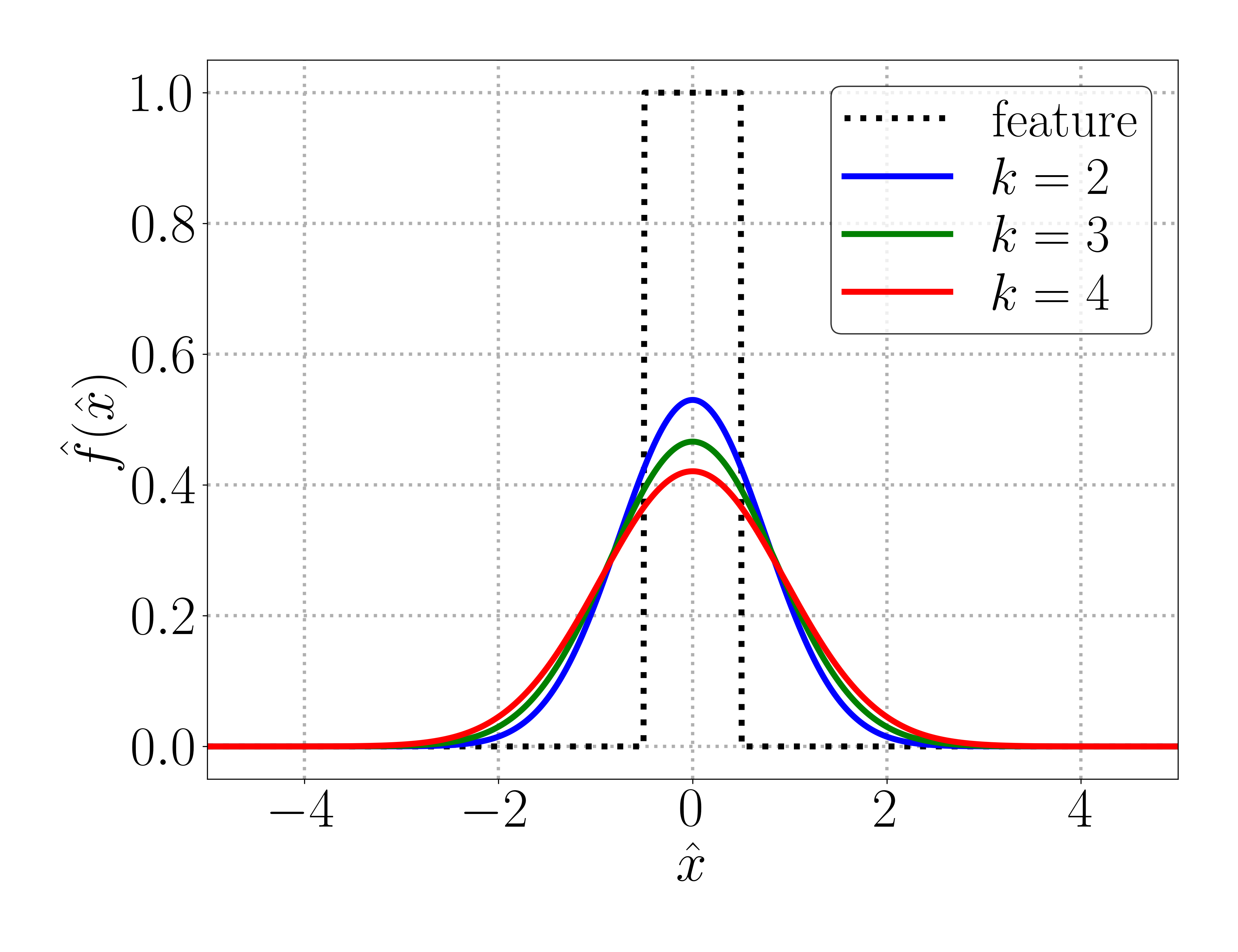
(b) $\hat{\ell}=\frac{\ell}{h}=1$

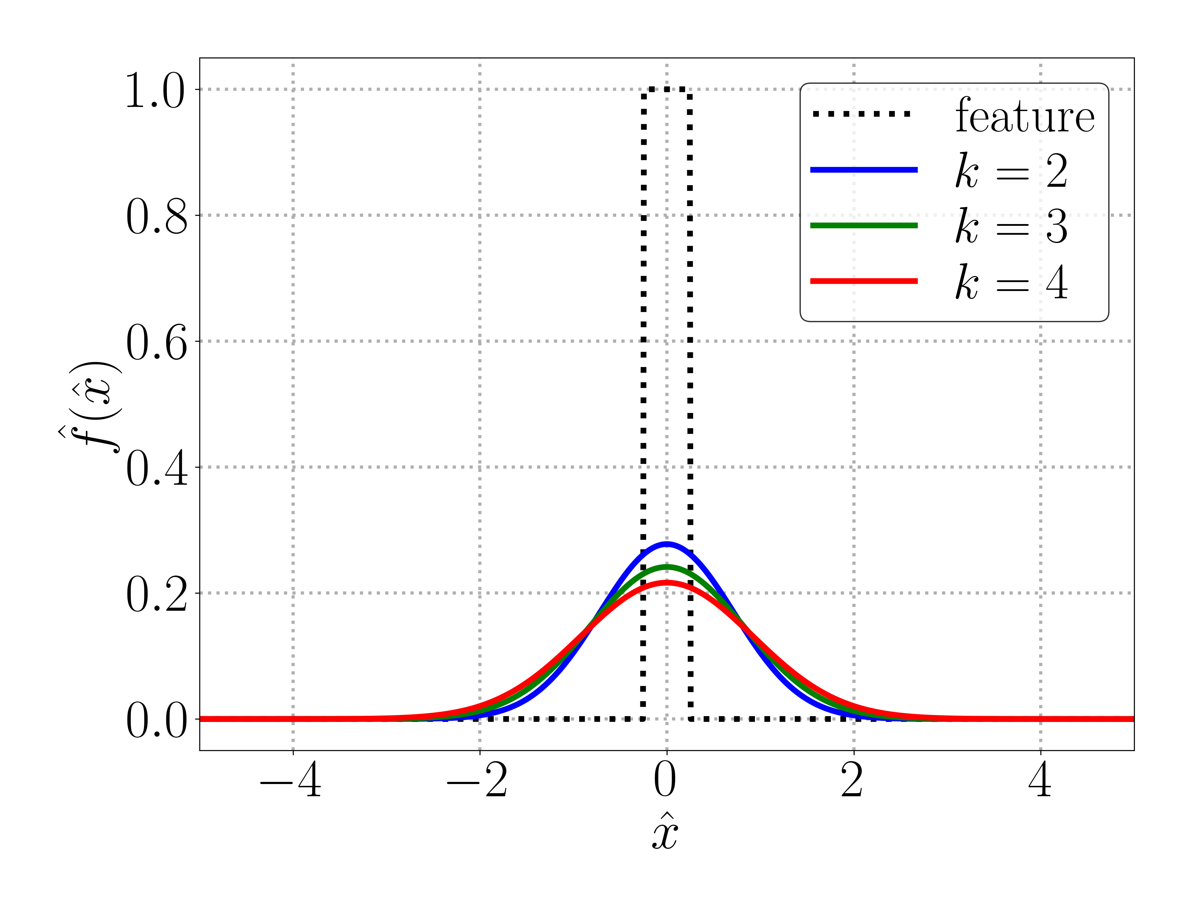
(c) $\hat{\ell}=\frac{\ell}{h}=\frac{1}{2}$

Figure 3: Smoothed level set approximation (3) of a geometric feature in the spatial domain, with $\hat{x}=x/h$, for various feature-size-to-mesh ratios, $\hat{\ell}=\ell/h$, and B-spline degrees.

2.2 Octree-based tessellation procedure

Our scan-based isogeometric analysis approach requires the construction of an explicit parametrization of the implicit level set domain (4). In this section we outline the segmentation procedure that we use to obtain an explicit parametrization of the domain and its (immersed) boundaries. This procedure, which is based on the octree subdivision approach introduced in the context of the Finite Cell Method in Ref. duster_finite_2008 (15), is illustrated in Fig. 4. In Section 2.2 we first discuss the employed octree procedure, after which the tessellation procedure used at the lowest level of subdivision is detailed in Section 2.2. Without loss of generality, in the remainder we will assume that the level set function $f$ is shifted such that $f_{\rm crit}=0$.

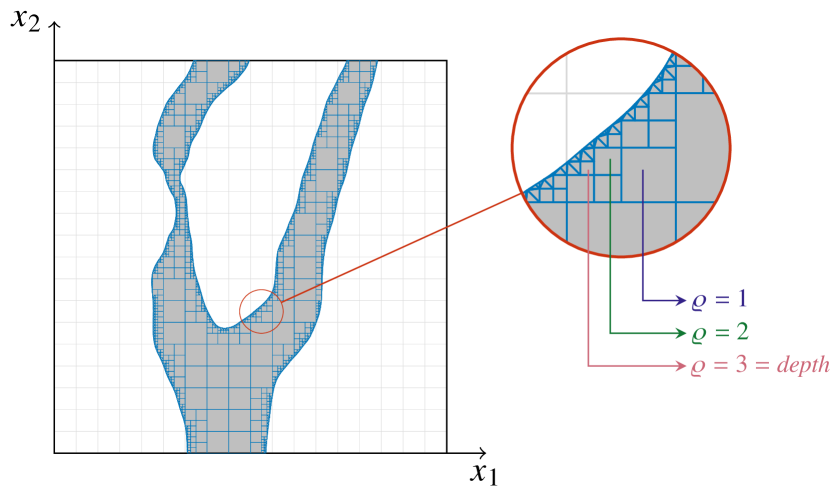
Figure 4: Illustration of the octree-based tessellation procedure to acquire an explicit parametrization of the immersed computational domain. The number of element subdivisions is indicated by $\varrho$, which is equal to the octree depth at the lowest level of bisectioning.

Octree subdivision

In our analysis framework we consider a regular mesh $\mathcal{T}_{\rm scan}^{h}$ that conforms to the scan domain $\Omega_{\rm scan}$. Each element in this mesh is a hyperrectangle (i.e., a line in one dimension, a rectangle in two dimensions, and a hexahedron in three dimensions) with size ${\boldsymbol{h}}=(h_{1},\ldots,h_{{d}})$ in each direction. Elements, $K$, that are intersected by the immersed boundary are trimmed, resulting in a partitioning, $\mathcal{P}_{K}$, of a cut element (see Fig. 4).

Algorithm 1 Function that trims an element based on an evaluate level set function

Input: array of level set values, octree depth, dimension of the element to be trimmed
      Output: element of type $\textit{Hyperrectangle}\cup\textit{Void}\cup\textit{WithChildren}\cup\textit{Mosaic}$

1:function trim_element(values, depth, dimension)

2:     if $\textbf{all}~{}\textit{values}>0$ then# All level set values are positive

3:         return Hyperrectangle(dimension)

4:     else if $\textbf{all}~{}\textit{values}\leq 0$ then# All level set values are non-positive

5:         return Void(dimension)

6:     else # Both positive and non-positive level set values

7:         if $\textit{depth}>0$ then # Recursively trim the element when $\textit{depth}>0$

8:              $\textit{withchildren\_element}\leftarrow\textsc{get\_withchildren\_element}(\textit{dimension})$

9:              for child in withchildren_element do

10:                  $\textit{child\_values}\leftarrow\textsc{get\_child\_values}(\textit{child},\textit{values})$

11:                  child $\leftarrow$ trim_element(child_values, $\textit{depth}-1$, dimension)

12:              end for

13:              return withchildren_element

14:         else # Terminate the recursion when $\textit{depth}=0$

15:              return $\textsc{get\_mosaic\_element}(\textit{values},\textit{dimension})$

16:         end if

17:     end if

18:end function

We employ the octree-based trimming procedure outlined in Alg. 1. This procedure follows a bottom-up approach varduhn_tetrahedral_2016 (41) in which the level set function (3) is sampled at the $2^{\textit{depth}}+1$ vertices of the octree in each direction for each element, where depth is the number of subdivision operations performed to detect the immersed boundary.

The trimming procedure takes the evaluated level set values, the subdivision depth and the dimension of the element as input arguments. If all level set values are positive (L2), the trim_element function retains the complete element in the mesh. If all level set values are non-positive (L4), the element is discarded. When some of the level set values are positive and some are non-positive (L6), this implies that the element is intersected by the immersed boundary. In this case, the element is subdivided (bisected) into $2^{d}$ children (L8). For each child a recursive call to the trim_element function is made (L11).

The recursive subdivision routine is terminated at the lowest level of subdivision, i.e., at $\textit{depth}=0$ (L14). Since our analysis approach requires the evaluation of functions on the immersed boundary, it is convenient to also obtain an explicit parametrization of this boundary. To obtain this parametrization, at the lowest level of subdivision we consider a tessellation procedure based on the level set values. The function get_mosaic_element that implements this procedure is discussed in Section 2.2.

Midpoint tessellation

At the lowest level of subdivision of the octree procedure, we perform a tessellation based on the $2^{d}$ level set values at that level. In the scope of our work, an important requirement for the tessellation procedure is that it is suitable for the consideration of interface problems. Practically, this means that if the procedure is applied to the negated level set function, a partitioning of the complementary part of the cell is obtained, with an immersed boundary that matches with that of the tessellation based on the original level set function (illustrated in Fig. 5(i)). Standard tessellation procedures, specifically Delaunay tessellation delaunay_sur_1934 (42), do not meet this requirement, as the resulting tessellation is always convex. When an immersed boundary tessellation is convex from one side, it is concave from the other side, meaning that it cannot be identically represented by the Delaunay tessellation. Another complication of Delaunay tessellation is its lack of uniqueness de_berg_computational_2008 (43), which in our applications results in non-matching interface tessellations.

Algorithm 2 Function that constructs a mosaic element based on level set values

Input: array of level set values, dimension of the element to be constructed
      Output: element of type $\textit{Mosaic}\cup\textit{Hyperrectangle}\cup\textit{Void}$

1:function get_mosaic_element($\textit{values},\textit{dimension}$)

2:     hyperrectangle $\leftarrow$ get_hyperrectangle(dimension)

3:     if $\textbf{all}~{}\textit{values}>0$ then# All level set values are positive

4:         return hyperrectangle

5:     else if $\textbf{all}~{}\textit{values}\leq 0$ then # All level set values are non-positive

6:         return Void

7:     else # Both positive and non-positive level set values

8:         boundaries $\leftarrow$ get_boundaries(hyperrectangle)

9:         for boundary in boundaries do

10:              $\textit{boundary\_values}\leftarrow\textsc{get\_boundary\_values}(\textit{boundary},\textit{values})$

11:              boundary $\leftarrow$ get_mosaic_element(boundary_values, $\textit{dimension}-1$)

12:         end for

13:         zero_points $\leftarrow$ get_zero_points(boundaries)

14:         midpoint $\leftarrow$ average(zero_points)

15:         mosaic_element $\leftarrow$ extrude_to_point(boundaries, midpoint)

16:         return mosaic_element

17:     end if

18:end function

To overcome the deficiencies associated with Delaunay tessellation, we have developed a dedicated tessellation procedure that suits the needs of our immersed analysis approach divi_error-estimate-based_2020 (32). We refer to the developed procedure as midpoint tessellation, which is illustrated in Figs. 5 and 6 for the two-dimensional and three-dimensional case, respectively. The get_mosaic_element function outlined in Alg. 2 implements our midpoint tessellation procedure. This function is called by the octree algorithm at the lowest level of subdivision (Alg. 1, L15), taking the $2^{d}$ level set values at the octree vertices as input. The function returns a tessellation of the octree cell that (approximately) fits to the immersed boundary.

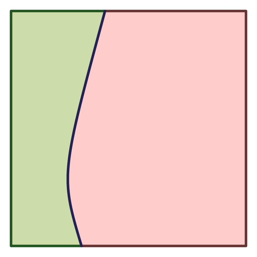
(a)

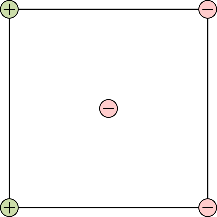
(b)

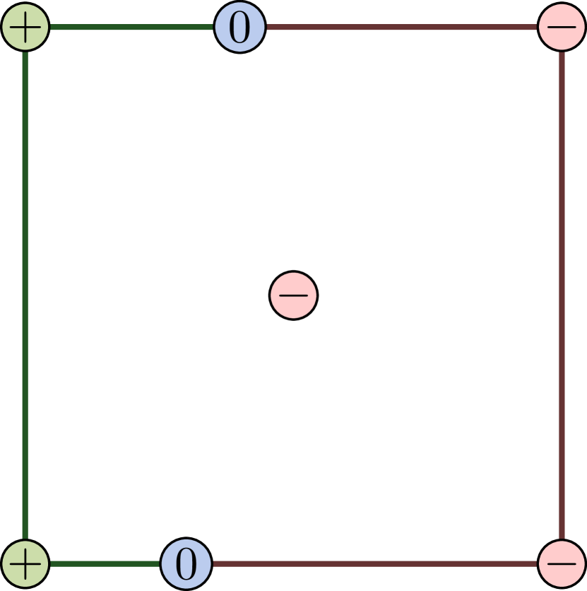
(c)

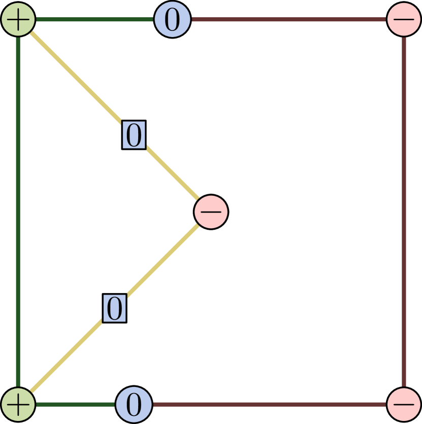
(d)

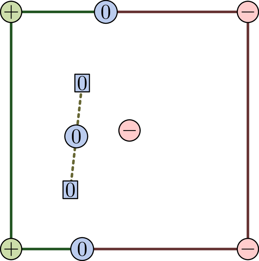
(e)

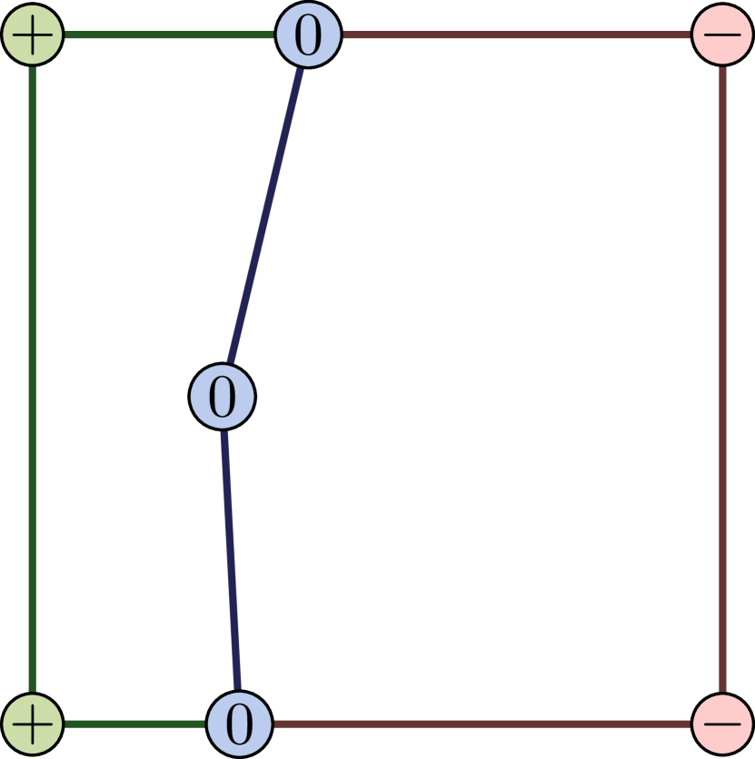
(f)

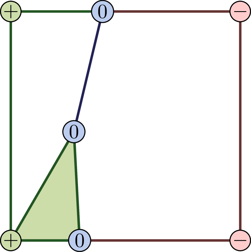
(g)

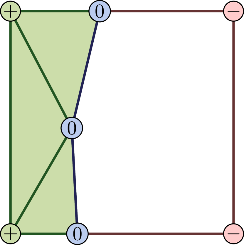
(h)

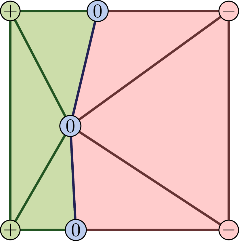
(i)

Figure 5: Schematic representation of the midpoint tessellation procedure for a two-dimensional case.

To explain Alg. 2, we first consider the two-dimensional case, which is illustrated in Fig. 5. The midpoint tessellation procedure commences with looping over all the edges of the element and recursively calling the get_mosaic_element function to truncate the edges that are intersected by the immersed boundary (L8-L12, Fig. 5(c)). A set of zero_points is then computed by linear interpolation of the level set function across the diagonals between the centroid of the rectangle and its vertices (L13, Fig. 5(d)), and the arithmetic average of these points is defined as the midpoint (L14, Fig. 5(e)). The tessellation is then created by extruding the (truncated) edges toward this midpoint (Figs. 5(g)-5(h)). Note that if this procedure is applied to the negated level set values, a tessellation of the complementary part of the rectangular element with a coincident immersed boundary is obtained (Fig. 5(i)).

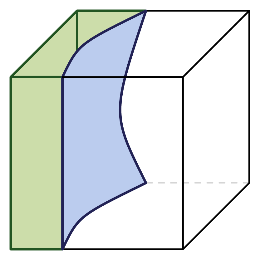
(a)

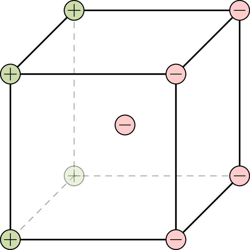
(b)

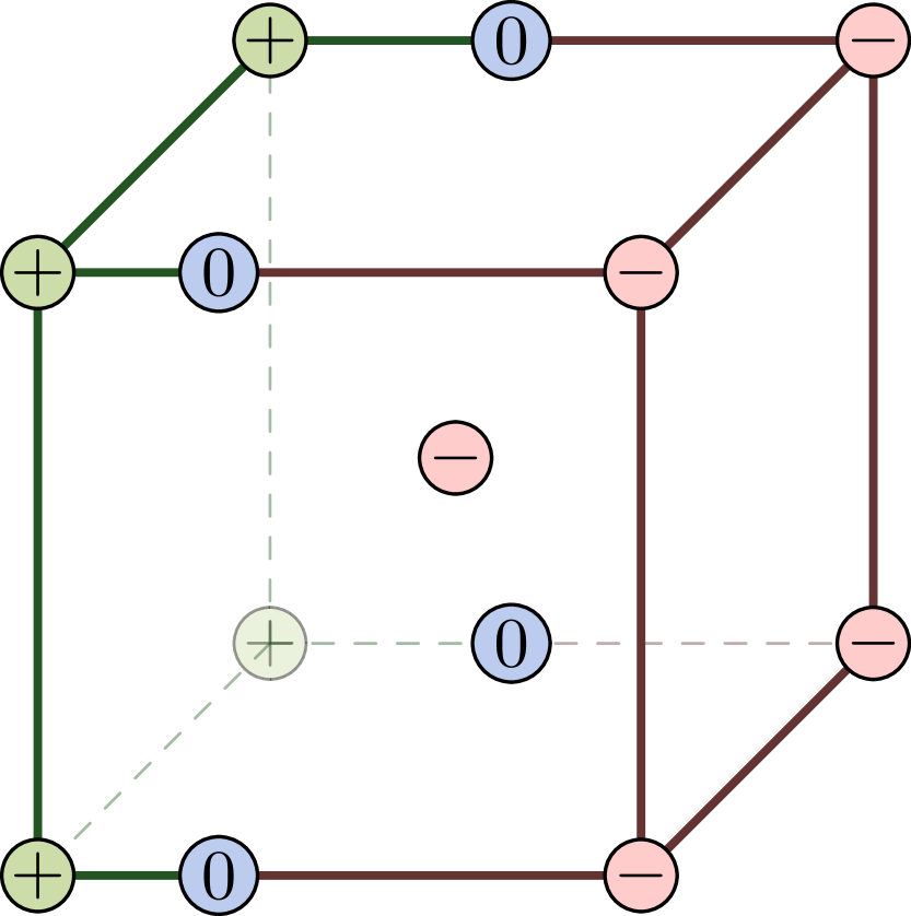
(c)

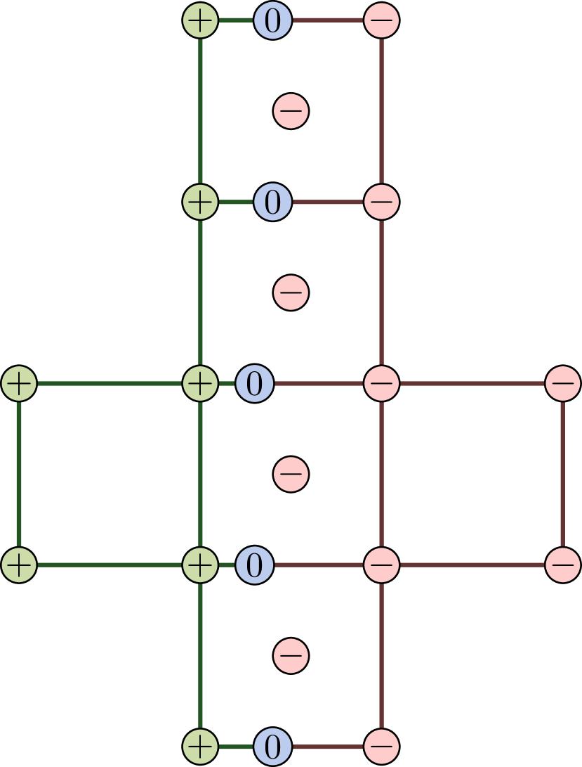
(d)

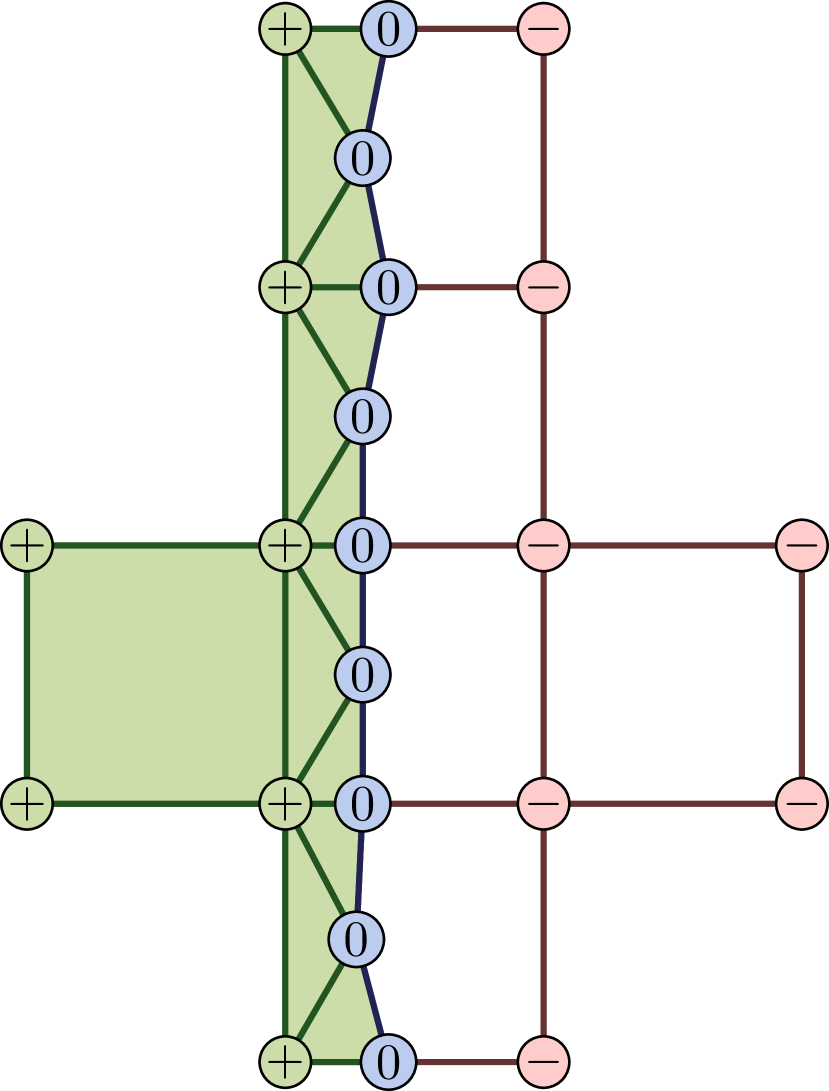
(e)

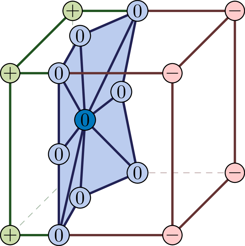
(f)

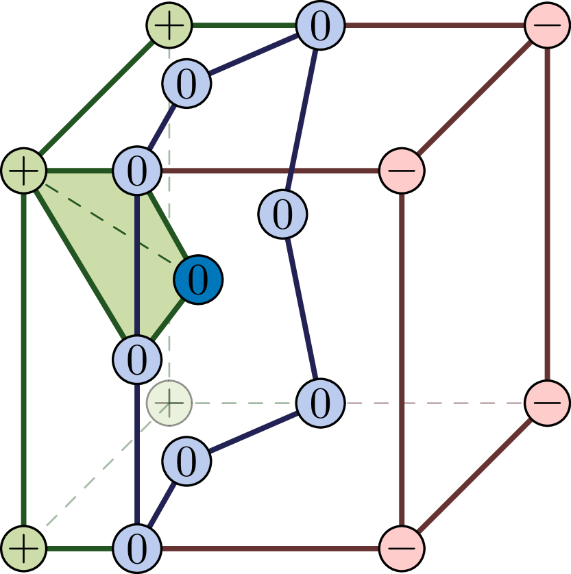
(g)

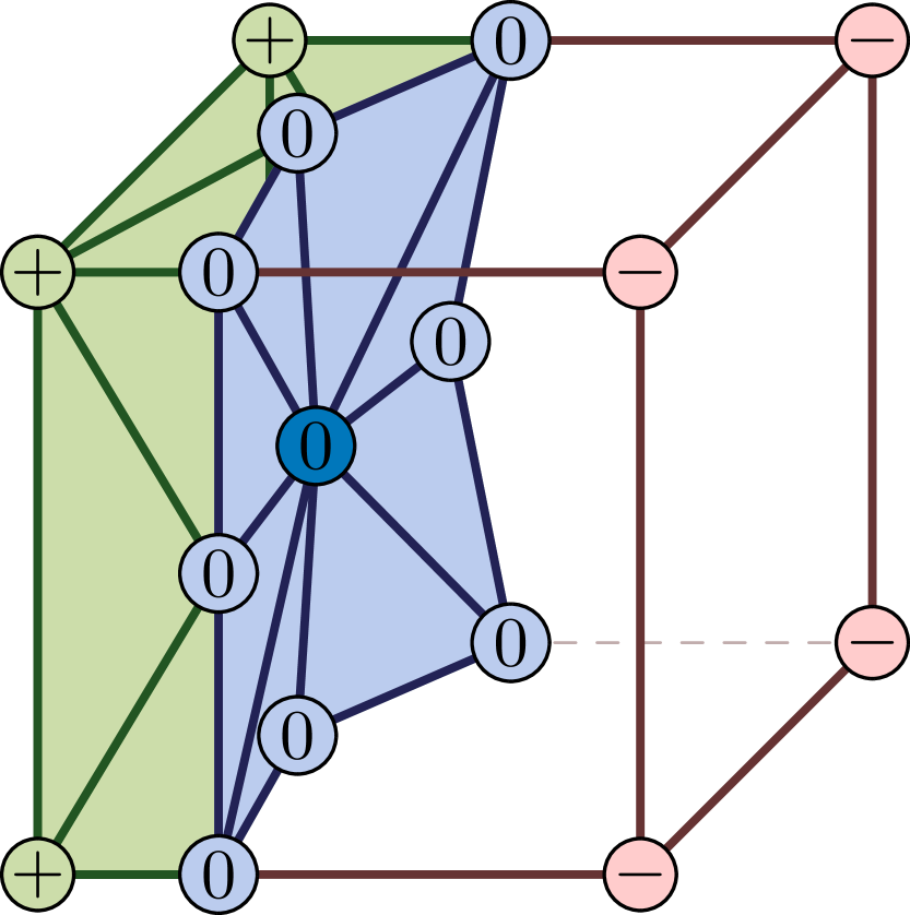
(h)

Figure 6: Schematic representation of the midpoint tessellation procedure for a three-dimensional case.

Since the tessellation algorithm recursively traverses the dimensions of the element, it can directly be extended to the three-dimensional case, as illustrated in Fig. 6. In three dimensions, all six faces of the element are tessellated by calling the get_mosaic_element function (L8-L12, Fig. 6(e)). Based on the diagonals between the centroid of the element and its vertices, zero level set points (L13) and a corresponding midpoint (L14) are then computed. The three-dimensional tessellation is finally constructed by extrusion of all (truncated) faces toward the midpoint (Fig. 6(g)-6(h)). As in the two dimensional case, a conforming interface is obtained when the procedure is applied to the negated level set values.

Remark 1 (Generalization to non-rectangular elements)

The algorithms presented in this section are presented for the case of hyperrectangles, i.e., a rectangle in two dimensions and a hexagon in three dimensions. The algorithms can be generalized to a broader class of element shapes (e.g., simplices, similar to Ref. varduhn_tetrahedral_2016 (41)). For the algorithms to be generalizable, the considered element must be able to define children (of the same type). Moreover, the element and its faces must be convex, so that the midpoint is guaranteed to be in the interior of the element. Note that this convexity requirement pertains to the shape of the untrimmed element, and not to the trimmed element.

2.3 Topology preservation

The spline-based segmentation procedure has been demonstrated to yield analysis-suitable domains for a wide range of test cases (see, e.g., Refs. verhoosel_image-based_2015 (25, 28, 44, 45, 32, 33, 36)). An example from Ref. divi_topology-preserving_2022 (33) is shown in Fig. 7. This example shows a carotid artery, obtained from a CT-scan. The scan data consists of 80 slices, separated by a distance of $400\,{\rm\mu m}$. Each slice image consists of $85\times 70$ voxels of size $300\times 300{\rm\mu m}^{2}$.

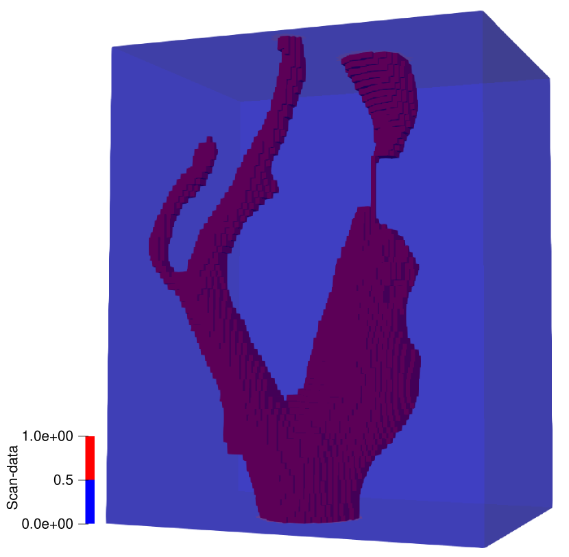
(a)

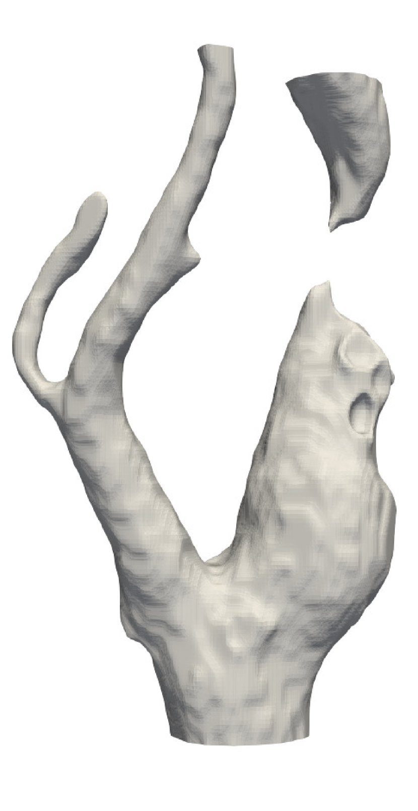
(b)

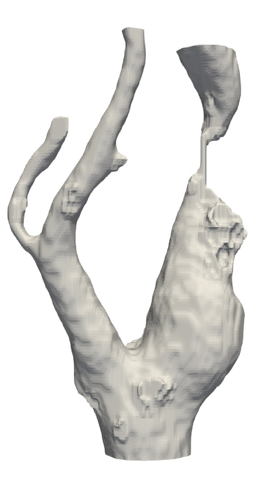
(c)

Figure 7: Example of the spline-based segmentation procedure for a scan-based image of a carotid artery. (7(a)) The original voxel data; (7(b)) the spline segmentation based on the voxel mesh, resulting in a topologically erroneous domain; and (7(c)) the spline segmentation after application of the topology-preservation algorithm.

When the spline-based segmentation procedure is performed using a B-spline level set function defined on the voxel grid, the result shown in Fig. 7(b) is obtained. Although the smoothing characteristic of the technique is overall beneficial, in the sense that it leads to smooth boundaries, comparison to the original voxel data in Fig. 7(a) shows that in this particular case the topology of the object is altered by the segmentation procedure. This can occur in cases where the features of the object to be described are not significantly larger in size than the voxels (i.e., the Nyquist criterion is not satisfied; see Section 2.1). In many cases, the altering of the topology of an object fundamentally changes the problem under consideration, and is therefore generally undesirable.

To avoid the occurrence of topological anomalies due to smoothing, a topology-preservation strategy has been developed in Ref. divi_topology-preserving_2022 (33). The developed strategy follows directly from the smoothing analysis presented in Section 2.1, which shows that features with a small relative length scale, $\hat{\ell}=\ell/h$, may be lost upon smoothing, cf. equation (10). Hence, topological features may be lost when the mesh size on which the B-spline level set is constructed is relatively large compared to the voxel size. The pivotal idea of the strategy proposed in Ref. divi_topology-preserving_2022 (33) is to detect topological anomalies by comparison of the segmented image (Fig. 7(b)) with the original voxel data (Fig. 7(a)) through a moving-window technique. In places where topological anomalies are detected, the mesh on which the smooth level set function is constructed is then refined locally (using THB-splines giannelli_thb-splines_2012 (37)). This locally increases the relative feature length scale, $\hat{\ell}$, such that the topology is restored (Fig. 7(c)).

3 Immersed isogeometric flow analysis

In this section we introduce an immersed discretization of the Stokes flow problem solved on a domain $\Omega\subset\mathbb{R}^{d}$ according to (4), attained through the scan-based segmentation procedure outlined above. The boundary, $\partial\Omega$, as illustrated in Fig. 8, is (partly) immersed, in the sense that it does not coincide with element boundaries.

The Stokes flow problem reads

$$\left\{\begin{aligned} -\nabla\cdot(2\mu\nabla^{s}{\boldsymbol{u}})+\nabla p&=\boldsymbol{f}&&\text{in }\Omega,\\ \nabla\cdot{\boldsymbol{u}}&=0&&\text{in }\Omega,\\ {\boldsymbol{u}}&=\boldsymbol{g}&&\text{on }\partial\Omega_{D},\\ 2\mu\left(\nabla^{s}{\boldsymbol{u}}\right)\boldsymbol{n}-p\boldsymbol{n}&=\boldsymbol{t}&&\text{on }\partial\Omega_{N},\end{aligned}\right.$$ (11)

with velocity ${\boldsymbol{u}}$, pressure $p$, constant viscosity $\mu$, body force $\boldsymbol{f}$, Dirichlet data $\boldsymbol{g}$ and Neumann data $\boldsymbol{t}$. The boundary is composed of a Neumann part, $\partial\Omega_{N}$, and a Dirichlet part, $\partial\Omega_{D}$, such that $\overline{\partial\Omega_{N}}\cup\overline{\partial\Omega_{D}}=\partial\Omega$ and $\partial\Omega_{N}\cap\partial\Omega_{D}=\emptyset$. The vector $\boldsymbol{n}$ in the last line denotes the outward-pointing unit normal to the boundary.

When discretizing the Stokes problem (11), the immersed setting poses various challenges: (i) Since the Dirichlet (e.g., no-slip) boundary is (partly) immersed, Dirichlet boundary conditions cannot be imposed strongly (i.e., by constraining degrees of freedom) hansbo_unfitted_2002 (46, 47); (ii) stability and conditioning issues can occur on unfavorably cut elements verhoosel_image-based_2015 (25, 44, 48, 19, 49); and (iii) elements which are known to be inf-sup stable in boundary-fitted finite elements (e.g., Taylor-Hood elements) can lose stability when being cut, resulting in oscillations in the velocity and pressure fields hoang_mixed_2017 (34).

To enable scan-based immersed isogeometric analyses, we have developed a stabilized formulation that addresses these challenges. In this formulation, Dirichlet boundary conditions are imposed weakly through Nitsche’s method hansbo_unfitted_2002 (46, 47). Ghost stabilization burman_ghost_2010 (17) is used to avoid conditioning and stability problems associated with unfavorably cut elements, and skeleton-stabilization is used to avoid inf-sup stability problems. Skeleton-stabilization also allows us to consider equal-order discretizations of the velocity and pressure spaces, simplifying the analysis framework. In Section 3.1 we first formalize the immersed analysis setting, after which the developed formulation is detailed in Section 3.2.

3.1 Immersed analysis setting

The physical domain is immersed in the (cuboid) scan domain, i.e., $\Omega_{\rm scan}\supset\Omega$, on which a locally refined scan mesh $\mathcal{T}^{h}_{\Omega_{\rm scan}}$ with elements $K$ is defined. Locally refined meshes can be constructed by sequential bisectioning of selections of elements in the mesh, starting from a Cartesian mesh, which will be discussed in Section 5.

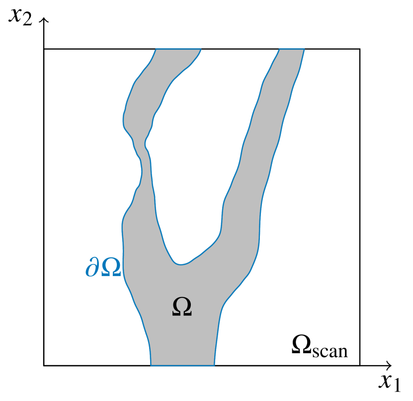
(a)

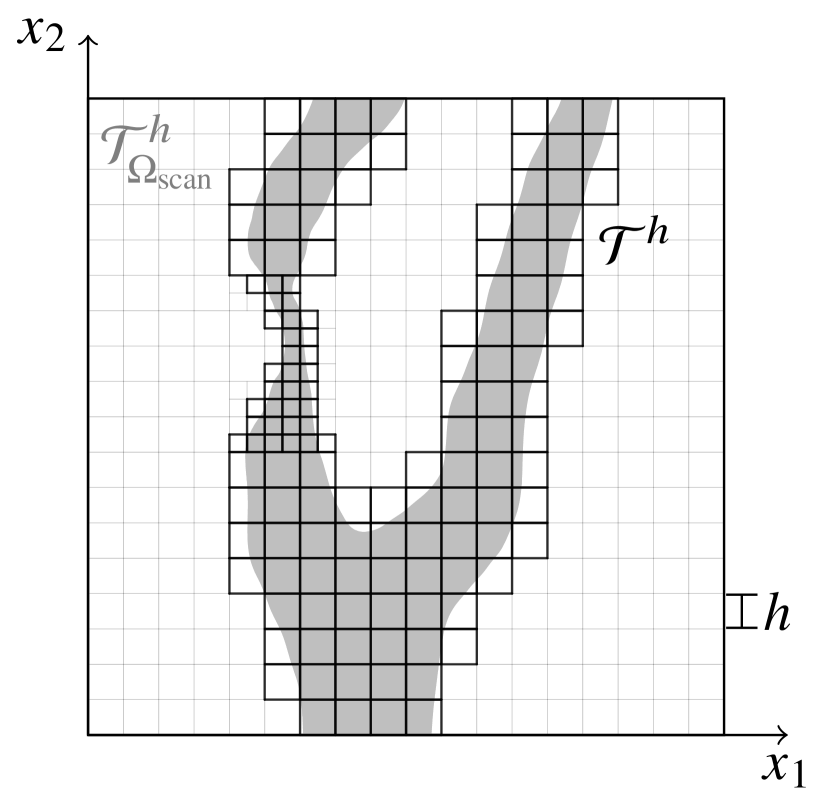
(b)

(c)

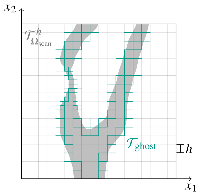
(d)

Figure 8: (8(a)) A physical domain $\Omega$ (gray), with boundary $\partial\Omega$ (blue), is embedded in the scan domain $\Omega_{\rm scan}$ (white). (8(b)) The background mesh $\mathcal{T}^{h}$, which consists of all elements that intersect the physical domain, is constructed by locally refining the ambient domain mesh $\mathcal{T}^{h}_{\Omega_{\rm scan}}$. The skeleton mesh, $\mathcal{F}_{\rm skeleton}$, and ghost mesh, $\mathcal{F}_{\rm ghost}$, are shown in panels (8(c)) and (8(d)), respectively.

Elements that do not intersect with the physical domain can be omitted, resulting in the locally refined (active) background mesh

$$\mathcal{T}^{h}:=\{K\,|\,K\in\mathcal{T}^{h}_{\Omega_{\rm scan}},K\cap\Omega\neq\emptyset\}.$$ (12)

The (active) background mesh is illustrated in Fig. 8(b). By cutting the elements that are intersected by the immersed boundary $\partial\Omega$, a mesh that conforms to the physical domain $\Omega$ is obtained:

$$\mathcal{T}^{h}_{\Omega}:=\{K\cap\Omega\,|\,K\in\mathcal{T}^{h}\}.$$ (13)

The tessellation procedure discussed in Section 2.2 provides a polygonal approximation of the immersed boundary $\partial\Omega$ through the set of boundary faces

$$\mathcal{T}^{h}_{\partial\Omega}:=\{E\subset\partial\Omega\,|\,E=\partial K\cap\partial\Omega,\,K\in\mathcal{T}^{h}_{\Omega}\}.$$ (14)

The considered formulation (see Section 3.2) incorporates stabilization terms formulated on the edges of the background mesh, which we refer to as the skeleton mesh

$$\mathcal{F}_{\rm skeleton}:=\{F=\partial K\cap\partial K^{\prime}\,|\ K,K^{\prime}\in\mathcal{T}^{h},K\neq K^{\prime}\}.$$ (15)

Note that the faces $F\in\mathcal{F}_{\rm skeleton}$ can be partially outside of the domain $\Omega$ and that the boundary of the background mesh is not part of the skeleton mesh. This skeleton mesh is illustrated in Fig. 8(c).

In addition to the skeleton mesh, we define the ghost mesh as the subset of the skeleton mesh with the faces that belong to an element intersected by the domain boundary, i.e.,

$$\mathcal{F}_{\rm ghost}:=\{F\cap\partial K\,|\,F\in\mathcal{F}_{\rm skeleton},K\in\mathcal{G}\},$$ (16)

where $\mathcal{G}:=\{K\in\mathcal{T}^{h}\mid K\cap\partial\Omega\neq\emptyset\}$ is the collection of elements in the background mesh that are crossed by the immersed boundary. The ghost mesh is illustrated in Fig. 8(d).

3.2 Stabilized formulation

To solve the Stokes problem (11) we discretize the velocity and pressure fields using truncated hierarchical B-splines giannelli_thb-splines_2012 (37, 50). THB-splines form a basis of degree $k$ and regularity $\alpha$ constructed over the locally-refined background mesh, $\mathcal{T}^{h}$, spanning the spline space

$$\mathcal{S}^{k}_{\alpha}(\mathcal{T}^{h})=\{N\in{}C^{\alpha}(\mathcal{T}^{h}):N|_{K}\in{}\mathcal{Q}^{k}(K),\,\forall{}K\in\mathcal{T}^{h}\},$$ (17)

with $\mathcal{Q}^{k}(K)$ the set of $d$-variate polynomials on the element $K$ constructed by the tensor-product of univariate polynomials of order $k$. We consider equal-order discretizations of the velocity and pressure spaces with optimal regularity THB-splines, i.e., $\alpha=k-1$:

$${{{\boldsymbol{u}}}^{h}} \in\boldsymbol{V}^{h}=[\mathcal{S}_{k-1}^{k}]^{d}\subset[H^{1}]^{d}, {{p}^{h}}\in Q^{h} =\mathcal{S}_{k-1}^{k}\subset L^{2}.$$ (18)

Note that the superscript $h$ is used to indicate that these fields are approximations obtained on a mesh with (local) element size $h$.

We consider the stabilized Bubnov-Galerkin formulation

$$\!\!\!\!\!\!\left\{\begin{aligned} &\text{Find}\>\boldsymbol{u}^{h}\in\boldsymbol{V}^{h}\>\text{and}\>p^{h}\in Q^{h}\>\text{such that:}\>&&\\ &a(\boldsymbol{u}^{h},\boldsymbol{v}^{h})+b(p^{h},\boldsymbol{v}^{h})+s_{\rm nitsche}(\boldsymbol{u}^{h},\boldsymbol{v}^{h})+s_{\rm ghost}(\boldsymbol{u}^{h},\boldsymbol{v}^{h})=f(\boldsymbol{v}^{h})&&\forall\boldsymbol{v}^{h}\in\boldsymbol{V}^{h}\\ &b(q^{h},\boldsymbol{u}^{h})-s_{\rm skeleton}(p^{h},q^{h})=g(q^{h})&&\forall q^{h}\in Q^{h}\end{aligned}\right.$$ (19)

where the bilinear and linear operators are defined as (see Ref. hoang_skeleton-stabilized_2019 (28) for details)

$$a(\boldsymbol{u}^{h},\boldsymbol{v}^{h}) :=2\mu(\nabla^{s}{{{\boldsymbol{u}}}^{h}},\nabla^{s}{{{\boldsymbol{v}}}^{h}})$$

$$\phantom{:=}-2\mu\left[\langle(\nabla^{s}{{{\boldsymbol{u}}}^{h}})\boldsymbol{n},{{{\boldsymbol{v}}}^{h}}\rangle_{\partial\Omega_{D}}+\langle(\nabla^{s}{{{\boldsymbol{v}}}^{h}})\boldsymbol{n},{{{\boldsymbol{u}}}^{h}}\rangle_{\partial\Omega_{D}}\right]$$ (20a)

$$b(p^{h},\boldsymbol{v}^{h}) :=-({{p}^{h}},\nabla\cdot{{{\boldsymbol{v}}}^{h}})+\langle p^{h},{{{\boldsymbol{v}}}^{h}}\cdot\boldsymbol{n}\rangle_{\partial\Omega_{D}}$$ (20b)

$$f(\boldsymbol{v}^{h}) :=(\boldsymbol{f},{{{\boldsymbol{v}}}^{h}})+\langle\boldsymbol{t},{{{\boldsymbol{v}}}^{h}}\rangle_{\partial\Omega_{N}}-2\mu\langle(\nabla^{s}{{{\boldsymbol{v}}}^{h}})\boldsymbol{n},\boldsymbol{g}\rangle_{\partial\Omega_{D}}$$ (20c)

$$g(q^{h}) :=\langle{{q}^{h}},\boldsymbol{g}\cdot\boldsymbol{n}\rangle_{\partial\Omega_{D}}$$ (20d)

$$s_{\rm nitsche}(\boldsymbol{u}^{h},\boldsymbol{v}^{h}) :=\langle\beta\mu h^{-1}({{{\boldsymbol{u}}}^{h}}-\boldsymbol{g}),{{{\boldsymbol{v}}}^{h}}\rangle_{\partial\Omega_{D}}$$ (20e)

$$s_{\rm ghost}(\boldsymbol{u}^{h},\boldsymbol{v}^{h}) :=\sum\limits_{F\in\mathcal{F}_{\rm ghost}}\int_{F}\gamma_{g}\mu h_{F}^{2k-1}\llbracket\partial_{n}^{k}\boldsymbol{u}^{h}\rrbracket\cdot\llbracket\partial_{n}^{k}\boldsymbol{v}^{h}\rrbracket\>{\rm d}S$$ (20f)

$$s_{\rm skeleton}(p^{h},q^{h}) :=\sum_{F\in\mathcal{F}_{\rm skeleton}}\int_{F}\gamma_{s}\mu^{-1}h_{F}^{2k+1}\llbracket\partial_{n}^{k}p^{h}\rrbracket\llbracket\partial_{n}^{k}q^{h}\rrbracket\>{\rm d}S$$ (20g)

where $(\cdot,\cdot)$ denotes the inner product in $L^{2}(\Omega)$, $\langle\cdot,\cdot\rangle_{\partial\Omega}$ denotes the inner product in $L^{2}(\partial\Omega)$, and $\llbracket\cdot\rrbracket$ denotes the interface jump operator. The parameters $\beta$, $\gamma_{g}$, and $\gamma_{s}$ denote the penalty constants for the Nitsche term, the ghost-stabilization term, and the skeleton-stabilization term, respectively.

To ensure stability and optimal approximation, the Nitsche stabilization term (20e) scales with the inverse of the (background) mesh size parameter, $h$ burman_cutfem_2015 (19). The Nitsche stability parameter $\beta$ should be selected appropriately, being large enough to ensure stability, while not being too large to cause locking-type effects (see, e.g., Refs. de_prenter_note_2018 (48, 51, 49)). The ghost-penalty operator in (20f) controls the $k^{\rm th}$-order normal derivative jumps over the interfaces of the elements which are intersected by the domain boundary $\partial\Omega$. Since in this contribution splines of degree $k$ with $C^{k-1}$-continuity are considered, only the jump in the $k^{\rm th}$ normal derivative is non-vanishing at the ghost mesh. The ghost-stabilization term scales with the size of the faces as $h_{F}^{2k-1}$. Appropriate selection of the parameter $\gamma_{g}$ corresponding with the Nitsche parameter, $\beta$, assures the stability of the formulation independent of the cut-cell configurations. To avoid loss of accuracy, the ghost-penalty parameter, $\gamma_{g}$, should also not be too large badia_linking_2022 (52).

The skeleton-stabilization operator (20g), proposed in Ref. hoang_skeleton-stabilized_2019 (28), penalizes jumps in higher-order pressure gradients. This ensures inf-sup stability of the equal-order velocity-pressure discretization, and resolves spurious pressure oscillations caused by cut elements. This spline-based skeleton-stabilization technique can be regarded as the higher-order continuous version of the interior penalty method proposed in Ref. burman_edge_2006 (53). To ensure stability and optimality, the operator (20g) scales with $h_{F}^{2k+1}$. The parameter $\gamma_{s}$ should be selected such that oscillations are suppressed, while the influence of the additional term on the accuracy of the solution remains limited. It is noted that since the inf-sup stability problem is not restricted to the immersed boundary, the skeleton stabilization pertains to all interfaces of the background mesh.

In our scan-based analysis workflow it is, from a computational effort point of view, generally impractical to evaluate the (integral) operators (20) exactly. The error of the Galerkin solution with inexact integration, $u^{h}_{\mathcal{Q}}=(\boldsymbol{u}^{h}_{\mathcal{Q}},p^{h}_{\mathcal{Q}})$, is then composed of two parts, viz.: (i) the discretization error, defined as the difference between the analytical solution, $u=(\boldsymbol{u},p)$, and the approximate Galerkin solution in the absence of integration errors, $u^{h}=(\boldsymbol{u}^{h},p^{h})$; and (ii) the inconsistency error related to the integration procedure, which is defined as the difference between the approximate solution in the absence of integration errors, $u^{h}$, and the Galerkin solution with integration errors, ${u}^{h}_{\mathcal{Q}}$. In practice, one needs to control both these error contributions in order to ensure the accuracy of a simulation result. From the perspective of computational effort, it is in general not optimal to make either one of the contributions significantly smaller than the other.

The decoupling of the geometry description from the analysis mesh provides the immersed (isogeometric) analysis framework with the flexibility to locally adapt the resolution of the solution approximation without the need to reparametrize the domain. To leverage this flexibility in the scan-based analysis setting, it is essential to automate the adaptivity procedure, as manual selection of adaptive cut-element quadrature rules and mesh refinement regions is generally impractical on account of the complex volumetric domains that are considered.

In our work we have developed error-estimation-based criteria that enable adaptive scan-based analyses. In Section 4 we first discuss an adaptive octree quadrature procedure used to reduce the computational cost associated with cut element integration. In Section 5 we then discuss a residual-based error estimator to refine the THB-spline approximation of the field variables only in places where this results in substantial accuracy improvements.

4 Adaptive integration of cut elements

From the perspective of computational effort, a prominent challenge in immersed finite element methods is the integration of the cut elements. While quadrature points can be constructed directly on all octree sub-cells (Section 2.2), this generally results in very expensive integration schemes, especially for three-dimensional problems divi_error-estimate-based_2020 (32). A myriad of techniques have been developed to make cut-element integration more efficient, an overview of which is presented in, e.g., Refs. abedian_performance_2013 (54, 32). In the selection of an appropriate cut element integration scheme one balances robustness (with respect to cut element configurations), accuracy, and expense.

In the context of scan-based analyses, we have found it most suitable to leverage the robustness of the octree procedure as much as possible. To improve the computational efficiency of the resulting quadrature rules, we have developed a procedure that adapts the number of integration points on each integration sub-cell, similar to the approach used in Ref. abedian_finite_2013 (55), as lower-order integration on very small sub-cells does not significantly reduce the accuracy.

4.1 Integration error estimate

The pivotal idea of our adaptive octree quadrature procedure is to optimally distribute integration points over the sub-cells using an error estimator based on Strang’s first lemma strang_analysis_2008 (35) (see also (ern_theory_2004, 56, Lemma 2.27)). In the immersed analysis setting, this lemma provides an upper bound for the error $u-u^{h}_{\mathcal{Q}}$. Following the derivation in Ref. divi_error-estimate-based_2020 (32) (to which we refer the reader for details), this error bound can be expressed in abstract form as

$$\left\|u-{u}^{h}_{\mathcal{Q}}\right\|_{W(h)}\leq\vphantom{\sum\limits_{K\in\mathcal{T}^{h}_{\Omega}}}\left(1+\frac{\left\|a^{h}\right\|_{W(h),V^{h}}}{\alpha^{h}}\right)\left\|u-\mathcal{I}^{h}u\right\|_{W(h)}+\frac{1}{\alpha^{h}}\sum\limits_{K\in\mathcal{T}^{h}_{\Omega}}\left(e_{K}^{a}+e_{K}^{f}\right),$$ (21)

where $\alpha^{h}$ denotes the inf-sup constant associated with the (aggregate) bilinear form $a^{h}:W^{h}\times V^{h}\rightarrow\mathbb{R}$, with trial and test velocity-pressure spaces $W^{h}$ and $V^{h}$, with $W(h)=\operatorname{span}{}\{u\}\oplus{}W^{h}$ the linear space containing the weak solution, $u$. The element-integration-error indicators associated with the (aggregate) bilinear form $a^{h}$ and (aggregate) linear form $f^{h}$ are respectively elaborated as

$$e_{K}^{a} =\operatornamewithlimits{sup\vphantom{p}}_{v^{h}_{K}\in{V}^{h}_{K}}{\frac{\left|\int_{K}A^{h}_{\Omega}(\mathcal{I}^{h}u,v^{h}_{K})(\boldsymbol{x}_{K})\,{\rm d}V-\sum\limits_{l=1}^{l_{K}}\omega^{l}_{K}A^{h}_{\Omega}(\mathcal{I}^{h}u,v^{h}_{K})(\boldsymbol{x}_{K}^{l})\right|}{\left\|v^{h}_{K}\right\|_{V^{h}_{K}}}},$$ (22a)

$$e_{K}^{f} =\operatornamewithlimits{sup\vphantom{p}}_{v^{h}_{K}\in{V}^{h}_{K}}{\frac{\left|\int_{K}F^{h}_{\Omega}(v^{h}_{K})(\boldsymbol{x})\,{\rm d}V-\sum\limits_{l=1}^{l_{K}}\omega^{l}_{K}F^{h}_{\Omega}(v^{h}_{K})(\boldsymbol{x}_{K}^{l})\right|}{\left\|v^{h}_{K}\right\|_{V^{h}_{K}}}},$$ (22b)

where $A^{h}_{\Omega}$ and $F^{h}_{\Omega}$ are the integrands corresponding to the volumetric terms in the bilinear form and linear form in the Galerkin problem, respectively, and where for each element $K$, the set $\{(\boldsymbol{x}_{K}^{l},\omega_{K}^{l})\}_{l=1}^{l_{K}}$ represents a quadrature rule. The norm $\|\cdot\|_{V_{K}^{h}}$ corresponds to the restriction of the space $V^{h}$ to the element $K$. We note that it has been assumed that integration errors associated with the boundary terms in the Galerkin problem are negligible in comparison to the errors in the volumetric terms, which is in line with the goal of optimizing the volumetric quadrature rules of cut elements.

It is desirable to apply a single integration scheme for all terms in the bilinear and linear forms and, hence, to treat the element-integration errors (22) in the same way. To do this, we note that the integrals between the absolute bars in the numerators of (22) constitute linear functionals on $V^{h}_{K}$. By the Riesz-representation theorem ern_theory_2004 (56), there exist functions $T^{a},T^{f}\in V^{h}_{K}$ such that

$$\int\limits_{K}T^{a}v^{h}_{K}\,{\rm d}V =\int\limits_{K}A^{h}_{\Omega}\left(\mathcal{I}^{h}u,v^{h}_{K}\right)\,{\rm d}V, \int\limits_{K}T^{f}v^{h}_{K}\,{\rm d}V =\int\limits_{K}F^{h}_{\Omega}\left(v^{h}_{K}\right)\,{\rm d}V,$$ (23)

for all $v^{h}_{K}\in V^{h}_{K}$. Assuming that the difference in applying the integral quadrature to the left- and right-hand-side members of (23) is negligible, it then holds that

$$e_{K}^{a} \leq\|T^{a}\|_{L^{2}(K)}\operatornamewithlimits{sup\vphantom{p}}_{T^{a},v^{h}_{K}\in V^{h}_{K}}{\frac{\left|\int_{K}T^{a}v^{h}_{K}\,{\rm d}V-\sum\limits_{l=1}^{l_{K}}\omega^{l}_{K}\left(T^{a}v^{h}_{K}\right)(\boldsymbol{x}_{K}^{l})\right|}{\|T^{a}\|_{L^{2}(K)}\|v^{h}_{K}\|_{V^{h}_{K}}}},$$ (24a)

$$e_{K}^{f} \leq\|T^{f}\|_{L^{2}(K)}\operatornamewithlimits{sup\vphantom{p}}_{T^{f},v^{h}_{K}\in V^{h}_{K}}{\frac{\left|\int_{K}T^{f}v^{h}_{K}\,{\rm d}V-\sum\limits_{l=1}^{l_{K}}\omega^{l}_{K}\left(T^{f}v^{h}_{K}\right)(\boldsymbol{x}_{K}^{l})\right|}{\|T^{f}\|_{L^{2}(K)}\|v^{h}_{K}\|_{V^{h}_{K}}}}.$$ (24b)

With both $T^{a}$ (resp. $T^{f}$) and $v^{h}_{K}$ in the polynomial space $V^{h}_{K}$, the product $T^{a}v^{h}_{K}$ (resp. $T^{f}v^{h}_{K}$) resides in the double-degree (normed) polynomial space $\mathcal{Q}_{K}^{2k}$. It then follows that

$$e_{K}^{a} \lesssim\|T^{a}\|_{L^{2}(K)}e_{K}^{p}, e_{K}^{f} \lesssim\|T^{f}\|_{L^{2}(K)}e_{K}^{p},$$ (25)

with the uniformly applicable polynomial integration error defined as

$$e_{K}^{p} =\operatornamewithlimits{sup\vphantom{p}}_{p_{K}\in\mathcal{Q}^{2k}_{K}}{\frac{\left|\int_{K}p_{K}(\boldsymbol{x}_{K})\,{\rm d}V-\sum\limits_{l=1}^{l_{K}}\omega^{l}_{K}{p_{K}}(\boldsymbol{x}_{K}^{l})\right|}{\|p_{K}\|_{P_{K}}}}$$

$$=\left|\int_{K}p_{K,{\rm max}}(\boldsymbol{x}_{K})\,{\rm d}V-\sum\limits_{l=1}^{l_{K}}\omega^{l}_{K}{p_{K,{\rm max}}}(\boldsymbol{x}_{K}^{l})\right|.$$ (26)

The supremizer can be evaluated in terms of a polynomial basis $\boldsymbol{\Phi}$ for the space $\mathcal{Q}_{K}^{2k}$ as (see Ref. divi_error-estimate-based_2020 (32) for a detailed derivation)

$$p_{K,{\rm max}}=\displaystyle\frac{\mathbf{\Phi}^{T}\mathbf{G}^{-1}(\boldsymbol{\xi}-\bar{\boldsymbol{\xi}})}{\|\boldsymbol{\xi}-\bar{\boldsymbol{\xi}}\|_{\mathbf{G}^{-1}}},$$ (27)

where $\boldsymbol{\xi}=\int_{K}\boldsymbol{\Phi}\,{\rm d}V$, $\bar{\boldsymbol{\xi}}=\sum_{l=1}^{l_{K}}\omega^{l}_{K}{\boldsymbol{\Phi}}(\boldsymbol{x}_{K}^{l})$, and $\mathbf{G}$ is the (positive definite) Gramian matrix associated with the inner product with which the polynomial space is equipped.

4.2 Quadrature optimization algorithm

The computable error definition (26) and the corresponding computable ”worst possible” function (27) form the basis of our adaptive integration procedure, which we summarize in Alg. 3 (a detailed version is presented in Ref. divi_error-estimate-based_2020 (32)). The developed optimization procedure is intended as a per-element preprocessing operation, which results in optimized quadrature rules for all cut elements in a mesh. Besides the partition, $\mathcal{P}_{K}$, of element, $K$, the procedure takes the order of the monomial basis, $\mathcal{Q}_{K}$, and stopping criterion (e.g., a prescribed number of integration points) as input.

Algorithm 3 Function to optimize the distribution of cut element quadrature points

Input: element partition, basis function order order, stopping criterion
      Output: optimized quadrature rule

1:function optimize_quadrature(partition, order, criterion)

2:     basis = get_monomial_basis(order)

3:     xi_exact = exact_integration(basis, order)

4:     gramian = get_gramian_matrix(basis, order)

5:     quadrature = initialize_quadrature(partition)

6:     while not criterion do # Adapt quadrature until the stopping criterion is met

7:         xi_quadrature = quadrature_integration(basis, quadrature)

8:         worst_function = get_worst_function(xi_exact, xi_quadrature, gramian, basis)

9:         indicators = initialize_indicators(partition)

10:         for subcell, indicator in zip(partition, indicators) do # Iterate over the sub-cells

11:              error = get_subcell_error(worst_function, quadrature)

12:              cost = get_subcell_cost(quadrature)

13:              indicator = get_subcell_indicator(subcell_error, subcell_cost)

14:         end for

15:         marking = mark_subcells(indicators) # Mark based on marking strategy

16:         quadrature = update_quadrature(quadrature, marking)

17:     end while

18:     return quadrature

19:end function

The procedure commences with the determination of the polynomial basis, $\mathbf{\Phi}$ (L2), the evaluation of the basis function integrals, $\boldsymbol{\xi}$ (L3), the computation of the gramian matrix, $\mathbf{G}$ (L4), and the initialization of the partition quadrature rule (L5). This initial quadrature rule corresponds to the case where the lowest order (one point) integration rule is used on each sub-cell in the partition. It is noted that the integral computations with full Gaussian quadrature for the basis and gramian are relatively expensive, but that the computational efficiency gains from the optimized integration scheme outweigh these costs when used multiple times.

The error-estimation-based quadrature optimization is then performed in an incremental fashion (L6), until the stopping criterion is met. Given the considered quadrature rule, the approximate basis integrals (L7) and worst possible function to integrate (27) (L8) are determined. Subsequently, for each sub-cell, $\wp$, in the partition (L10), on L11 the sub-cell error indicators

$$e_{\wp}^{p} =\left|\int_{\wp}p_{K,{\rm max}}(\boldsymbol{x}_{K})\,{\rm d}V-\sum\limits_{l\in\mathcal{I}_{\wp}}\omega^{l}_{K}{p_{K,{\rm max}}}(\boldsymbol{x}_{K}^{l})\right|$$ (28)

are computed. In this expression, $\mathcal{I}_{\wp}$, is the set of indices corresponding to integration points on the sub-cell $\wp$. Note that the sum of the sub-cell errors, $e_{\wp}^{p}$, provides an upper bound for the element integration error (26). Sub-cell indicators are then computed (L13) by weighing the sub-cell errors with the costs associated with increasing the quadrature order on a particular sub-cell, as evaluated on L12 (see Ref. divi_error-estimate-based_2020 (32) for details).

Once the indicators have been computed for all sub-cells in the partition, the sub-cells with the largest indicators are marked for increasing the number of integration points (L15). We propose two marking strategies, viz. a sub-cell marking strategy in which only the sub-cell with the highest indicator is marked, and an octree-level marking strategy in which all sub-cells in the octree level with the highest error are marked. After marking, the quadrature order on the marked sub-cells is increased (L16).

4.3 Optimized quadrature results

A detailed study of the error-estimation-based quadrature optimization scheme is presented in Ref. divi_error-estimate-based_2020 (32). We here reproduce a typical result for a unit square with a circular exclusion, as illustrated in Fig. 9. To assess the performance of the developed adaptive integration technique, we study its behavior in terms of integration accuracy versus the number of integration points.

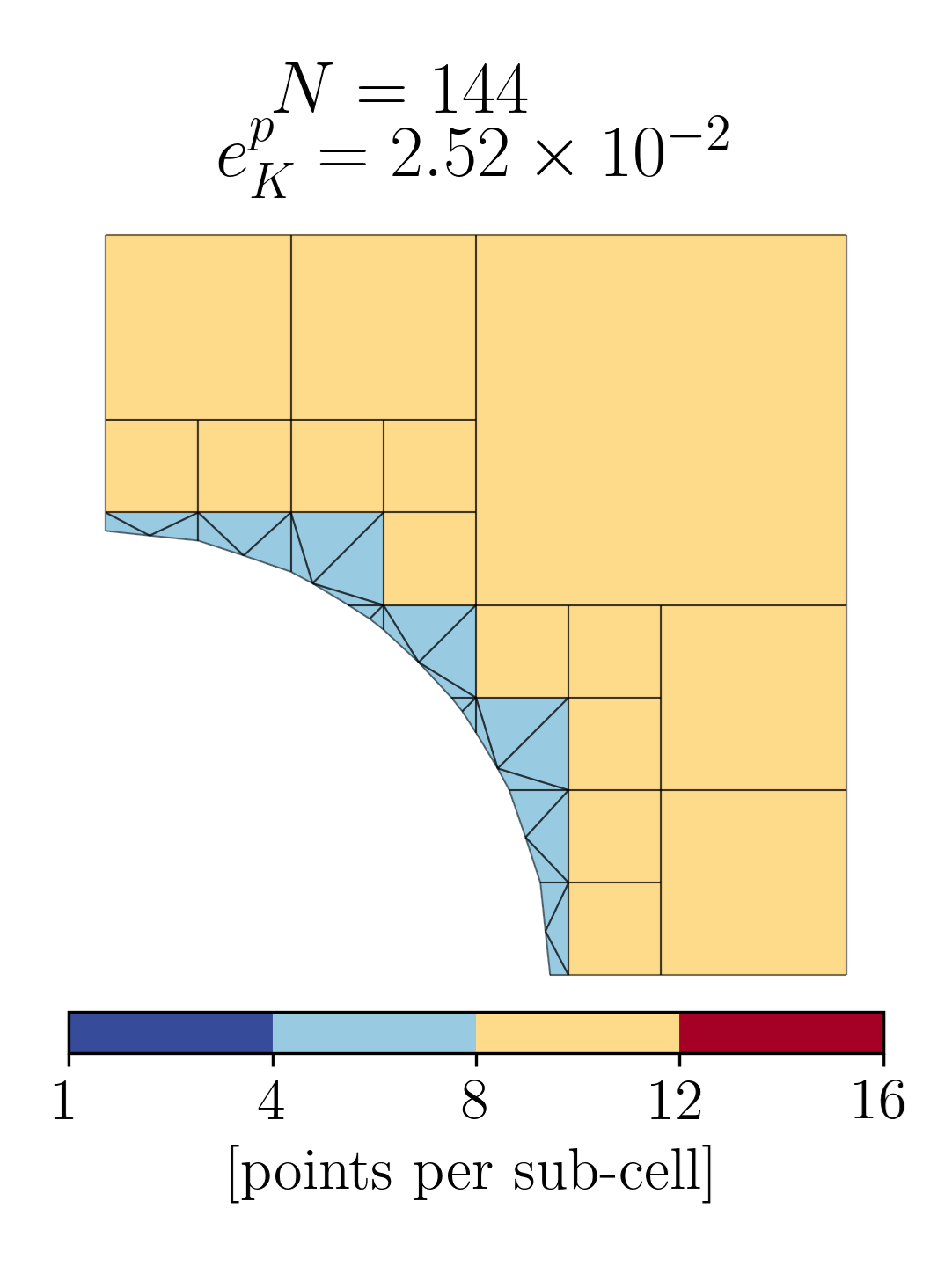
(a) Equal-order Gauss

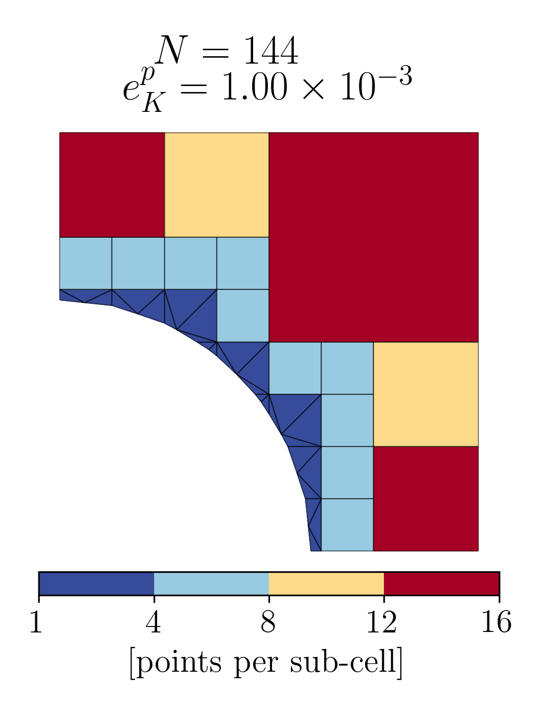
(b) Optimal integration

Figure 9: Distribution of integration points over a cut element with $144$ points, comparing the case of (9(a)) an equal-order Gauss scheme, and (9(b)) optimally distributed Gauss points using the sub-cell marking strategy. Note that the error is reduced by a factor of 25 by using the sub-cell marking strategy.

Fig. 10(a) displays the integration error as evolving during the optimization procedure when using the sub-cell marking strategy. The non-optimized case in which the same integration scheme is considered on each sub-cell is displayed for reference. As can be seen, the error associated to the same number of integration points is substantially lowered using the adaptive integration procedure. For example, for the case where $144$ integration points are considered, the error corresponding to the non-optimized second-order Gauss scheme is equal to $2.52\times 10^{-2}$, while the error corresponding to the optimized quadrature is equal to $1.00\times 10^{-3}$, i.e., a factor 25 reduction in error. Fig. 9 displays the distribution of the integration points over the sub-cells for the equal-order Gauss scheme and the optimized case, which clearly demonstrates that the significant reduction in error is achieved by assigning more integration points to the larger sub-cells before introducing additional points in the smaller sub-cells. From Fig. 10(a) it is also observed that when the optimization algorithm is terminated at a fixed error of, e.g., $e_{K}^{p}\approx 1\cdot 10^{-2}$, the number of integration points $N$ using the optimized integration scheme is reduced substantially (in this case from 303 to 83, i.e., a factor of almost 4). Even substantially bigger gains are observed in three-dimensional cases divi_error-estimate-based_2020 (32).

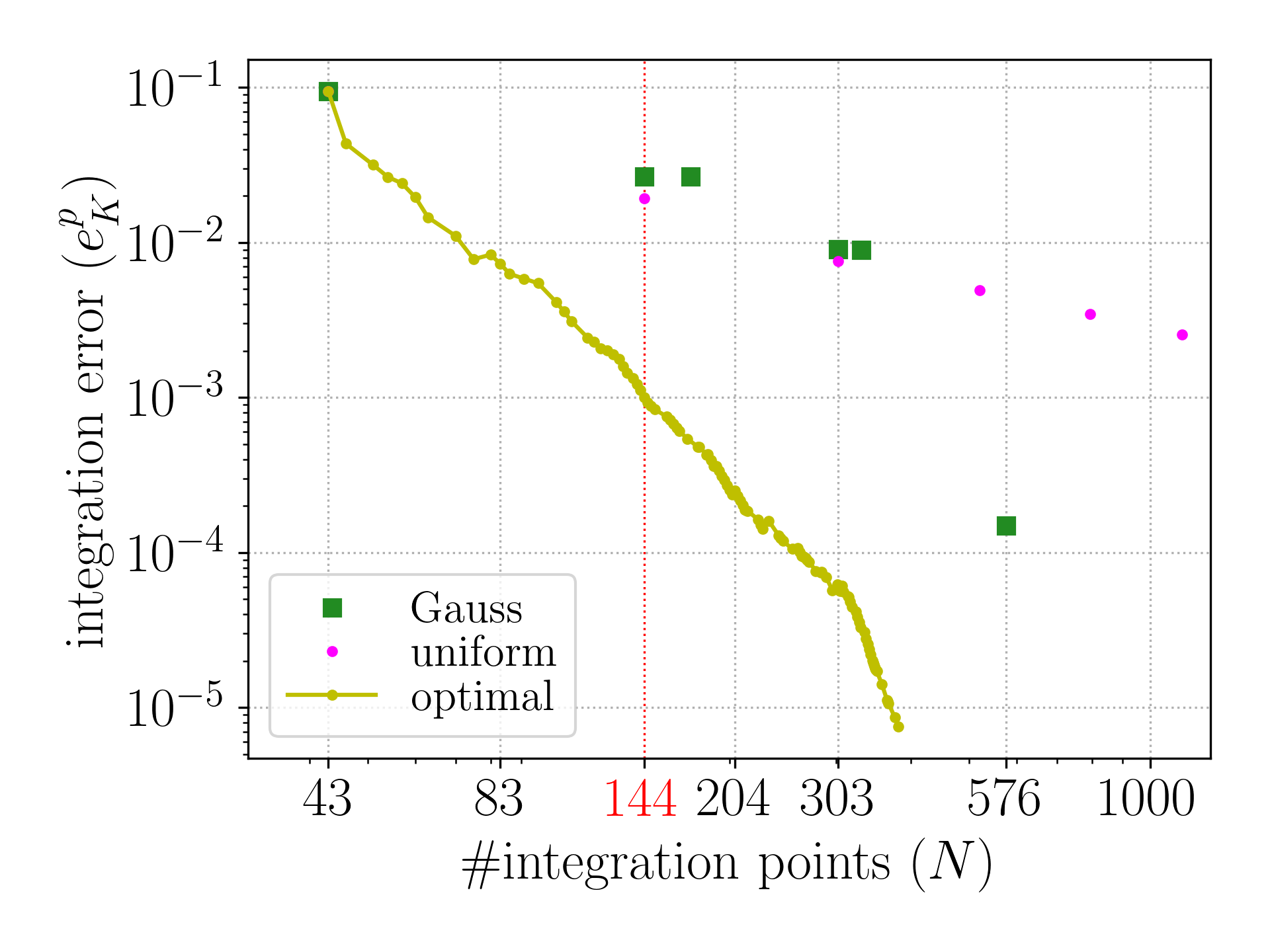
(a)

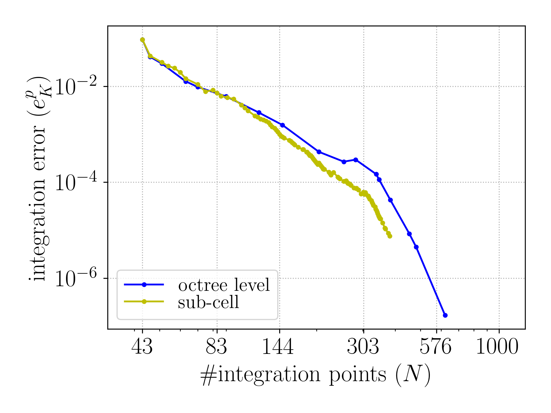
(b)

Figure 10: Integration error vs. the number of integration points. (10(a)) Comparison of the optimized quadrature results with (non-optimized) equal-order integration. (10(b)) Comparison of the sub-cell and octree-level marking strategies.

From the quadrature updating patterns that emerge from the sub-cell marking strategy it is observed that, as a general trend, integration orders are increased on a per-octree-level basis. This is explained by the fact that the indicators scale with the volume of the sub-cells. Based on this observation it was anticipated that an octree-level marking strategy could be very efficient, in the sense that it would yield a similar quadrature update pattern as the sub-cell marking, but that it would need fewer iterations by virtue of marking a larger number of sub-cells per step. Fig. 10(b) compares the marking strategies, conveying that the octree-level marking indeed closely follows the sub-cell marking.

Although the computational effort of the quadrature optimization algorithm is worthwhile when one wants to re-use a quadrature rule multiple times, considerable computational effort is involved. In addition, one has to set up a suitable code to determine the optimal distributions for arbitrarily cut elements. Considering this, one may not be interested in obtaining the optimized distributions of the points, but may instead want a simple rule of thumb to select the quadrature on a cut element; see, e.g., Refs. abedian_finite_2013 (55, 57). Using our quadrature optimization algorithm, in Ref. divi_error-estimate-based_2020 (32) we studied the effectivity of rules of thumb in which the order of integration is lowered with the octree depth. Although the rule-of-thumb schemes are, as expected, outperformed by the optimized schemes, they generally do provide an essential improvement in accuracy per integration point compared to equal-order integration. This observed behavior is explained by the fact that the rules of thumb qualitatively match the results of the optimization procedure.

5 Adaptive THB-spline refinement

To leverage the flexibility of the immersed simulation paradigm with respect to refining the mesh independent of the geometry, an automated mesh adaptivity strategy is required. Various adaptivity strategies have been considered in the context of immersed methods, an overview of which is presented in, e.g., Ref. divi_residual-based_2022 (36). These refinement strategies can be categorized as either feature-based methods (refinements are based on, e.g., sharp gradients in the solution or high-curvature boundary regions) or methods based on error estimates (e.g., residual-based or goal-oriented methods).

To develop a generic adaptive procedure for scan-based analyses, we have constructed a residual-based a posteriori error estimator. In our isogeometric analysis approach we employ truncated hierarchical B-splines (THB-splines) giannelli_thb-splines_2012 (37, 50) to locally refine the (volumetric) background mesh.

5.1 Residual-based error estimation

On account of the immersed boundary terms in the formulation (Section 3), it is not well-posed in the infinite dimensional setting. Upon appropriate selection of the stabilization parameters, the (mixed) Galerkin formulation of the Stokes problem is well-posed with respect to the mesh-dependent norm (see Ref. divi_residual-based_2022 (36) for details)

$$\left|\kern-1.07639pt\left|\kern-1.07639pt\left|v^{h}\right|\kern-1.07639pt\right|\kern-1.07639pt\right|^{2}=\left|\kern-1.07639pt\left|\kern-1.07639pt\left|(\boldsymbol{v}^{h},q^{h})\right|\kern-1.07639pt\right|\kern-1.07639pt\right|^{2}=\left|\kern-1.07639pt\left|\kern-1.07639pt\left|{{{\boldsymbol{v}}}^{h}}\right|\kern-1.07639pt\right|\kern-1.07639pt\right|^{2}_{u}+\left|\kern-1.07639pt\left|\kern-1.07639pt\left|{{q}^{h}}\right|\kern-1.07639pt\right|\kern-1.07639pt\right|^{2}_{p},$$ (29)

with

$$\left|\kern-1.07639pt\left|\kern-1.07639pt\left|{{{\boldsymbol{v}}}^{h}}\right|\kern-1.07639pt\right|\kern-1.07639pt\right|^{2}_{u} :=\lVert\mu^{\frac{1}{2}}\nabla^{s}\boldsymbol{v}^{h}\rVert_{L^{2}(\mathcal{T})}^{2}+\lVert\beta^{-\frac{1}{2}}h^{\frac{1}{2}}\mu^{\frac{1}{2}}\partial_{n}\boldsymbol{v}^{h}\rVert_{L^{2}(\partial\Omega_{D})}^{2}$$

$$\phantom{:=}+\lVert\beta^{\frac{1}{2}}h^{-\frac{1}{2}}\mu^{\frac{1}{2}}\boldsymbol{v}^{h}\rVert_{L^{2}(\partial\Omega_{D})}^{2}+\sum\limits_{F\in\mathcal{F}_{\rm ghost}}\lVert\gamma_{g}^{\frac{1}{2}}h_{F}^{k-\frac{1}{2}}\mu^{\frac{1}{2}}\llbracket\partial_{n}^{k}\boldsymbol{v}^{h}\rrbracket\rVert_{L^{2}(F)}^{2},$$ (30a)

$$\left|\kern-1.07639pt\left|\kern-1.07639pt\left|{{q}^{h}}\right|\kern-1.07639pt\right|\kern-1.07639pt\right|^{2}_{p} :=\lVert\mu^{-\frac{1}{2}}q^{h}\rVert_{L^{2}(\mathcal{T})}^{2}+\sum\limits_{F\in\mathcal{F}_{\rm skeleton}}\lVert\gamma_{s}^{\frac{1}{2}}h_{F}^{k+\frac{1}{2}}\mu^{-\frac{1}{2}}\llbracket\partial_{n}^{k}q^{h}\rrbracket\rVert_{L^{2}(F)}^{2}.$$ (30b)

We refer to this mesh-dependent norm as the energy norm and use it to construct an a posterior error estimator for the discretization error, $u-u^{h}$.

Since, in the considered immersed setting, stability can only be shown in the discrete setting, we define the solution error with respect to the solution in the order-elevated space $\widehat{u}^{h}\in\widehat{V}^{h}$. The space $\widehat{V}^{h}$ is defined on the same mesh and with the same regularity as the space $V^{h}$, but with the order of the basis elevated in such a way that $\widehat{V}^{h}\supset V^{h}$. It is then assumed that

$$\left|\kern-1.07639pt\left|\kern-1.07639pt\left|\widehat{u}^{h}-{u^{h}}\right|\kern-1.07639pt\right|\kern-1.07639pt\right|\approx\left|\kern-1.07639pt\left|\kern-1.07639pt\left|u-{u^{h}}\right|\kern-1.07639pt\right|\kern-1.07639pt\right|.$$ (31)

We note that additional stabilization terms are required to retain stability in the order-elevated space. In principle this means that the operators (20) need to be augmented, but we assume that for the solution in the order-elevated space these terms are negligible. Similar assumptions, referred to as saturation assumptions, have been considered in, e.g., Refs. becker_finite_2003 (58, 59, 60). Note that the refined space is only used to provide a proper functional setting for the error estimator and that it is not required to perform computations in this space.

To construct an estimator for the error (31), it can be bound from above by

$$\left|\kern-1.07639pt\left|\kern-1.07639pt\left|\widehat{u}^{h}-{u^{h}}\right|\kern-1.07639pt\right|\kern-1.07639pt\right|\lesssim\operatornamewithlimits{sup\vphantom{p}}_{\widehat{v}^{h}\in\widehat{V}^{h}\setminus\{0\}}\frac{a^{h}(\widehat{u}^{h}-u^{h},\widehat{v}^{h})}{\left|\kern-1.07639pt\left|\kern-1.07639pt\left|\widehat{v}^{h}\right|\kern-1.07639pt\right|\kern-1.07639pt\right|}=\operatornamewithlimits{sup\vphantom{p}}_{\widehat{v}^{h}\in\widehat{V}^{h}\setminus\{0\}}\frac{r^{h}(\widehat{v}^{h})}{\left|\kern-1.07639pt\left|\kern-1.07639pt\left|\widehat{v}^{h}\right|\kern-1.07639pt\right|\kern-1.07639pt\right|},$$ (32)

where the aggregate residual (i.e., the combined velocity-pressure residual) is defined as

$$r^{h}(\widehat{v}^{h}) :=r^{h}(u^{h})(\widehat{v}^{h}):=f^{h}(\widehat{v}^{h})-a^{h}(u^{h},\widehat{v}^{h}),$$ (33)

with aggregate operators $a^{h}$ and $f^{h}$ (see Ref. divi_residual-based_2022 (36) for details).

We propose an error estimator pertaining to the background mesh, $\mathcal{T}^{h}$, which bounds the error in the energy norm (32) as

$$\mathcal{E}=\sqrt{\sum\limits_{K\in\mathcal{T}^{h}}\eta_{K}^{2}}\gtrsim\operatornamewithlimits{sup\vphantom{p}}_{\widehat{v}^{h}\in\widehat{V}^{h}\setminus\{0\}}\frac{r^{h}(\widehat{v}^{h})}{\left|\kern-1.07639pt\left|\kern-1.07639pt\left|\widehat{v}^{h}\right|\kern-1.07639pt\right|\kern-1.07639pt\right|}\gtrsim\left|\kern-1.07639pt\left|\kern-1.07639pt\left|\widehat{u}^{h}-{u^{h}}\right|\kern-1.07639pt\right|\kern-1.07639pt\right|,$$ (34)

where the element-wise error indicators, $\eta_{K}$, will serve to guide an adaptive refinement procedure.

To derive the error indicators, the residual (33) is considered with the operators defined as in (20). Following the derivation of Ref. divi_residual-based_2022 (36), the indicators are defined as

$$\eta_{K}^{2} =\mu^{-1}h_{K}^{2}\|\boldsymbol{r}_{{\rm int},{\boldsymbol{u}}}^{h}\|_{L^{2}(K\cap\Omega)}^{2}+\mu\|r_{{\rm int},p}^{h}\|_{L^{2}(K\cap\Omega)}^{2}$$ (35)

$$\phantom{=}+\mu^{-1}h_{K}\|{\boldsymbol{r}_{\rm neumann}^{h}}\|_{L^{2}({K\cap\partial\Omega_{N}})}^{2}+9\mu h_{K}^{-1}\|\boldsymbol{r}_{\rm nitsche}^{h}\|_{L^{2}({K\cap\partial\Omega_{D}})}^{2}$$

$$\phantom{=}+\sum_{F\in\mathcal{F}_{\rm skeleton}}\mu^{-1}h_{K}\|\boldsymbol{r}_{\rm jump}^{h}\|_{L^{2}({\partial K\cap F})}^{2}+\mu\beta^{2}h_{K}^{-1}\|\boldsymbol{r}_{\rm nitsche}^{h}\|_{L^{2}(K\cap\partial\Omega_{D})}^{2}\Bigg{.}$$

$$\phantom{=}+\sum\limits_{F\in\mathcal{F}_{\rm ghost}^{K}}\mu\gamma_{g}^{2}h_{F}^{2k-1}\|\boldsymbol{r}_{\rm ghost}^{h}\|_{L^{2}(\partial K\cap F)}^{2}$$

$$\phantom{=}+\sum\limits_{F\in\mathcal{F}_{\rm skeleton}^{K}}\mu^{-1}\gamma_{s}^{2}h_{F}^{2k+1}\|r_{\rm skeleton}^{h}\|_{L^{2}(\partial K\cap F)}^{2},$$

where

$$\boldsymbol{r}_{{\rm int},{\boldsymbol{u}}}^{h} :=\boldsymbol{f}+\nabla\cdot\left(2\mu\nabla^{s}{{{\boldsymbol{u}}}^{h}}\right)-\nabla{{p}^{h}},$$ (36a)

$$r_{{\rm int},p}^{h} :=\nabla\cdot{{{\boldsymbol{u}}}^{h}},$$ (36b)

$${\boldsymbol{r}_{\rm neumann}^{h}} :=\boldsymbol{t}-\left(2\mu\nabla^{s}{{{\boldsymbol{u}}}^{h}}\right)\boldsymbol{n}+{{p}^{h}}\boldsymbol{n},$$ (36c)

$$\boldsymbol{r}_{\rm nitsche}^{h} :=\boldsymbol{g}-{{{\boldsymbol{u}}}^{h}},$$ (36d)

$$\boldsymbol{r}_{\rm jump}^{h} :=\tfrac{1}{2}\llbracket\left(2\mu\nabla^{s}{{{\boldsymbol{u}}}^{h}}\right)\boldsymbol{n}\rrbracket,$$ (36e)

$$\boldsymbol{r}_{\rm ghost}^{h} :=\tfrac{1}{2}\llbracket\partial_{n}^{k}{{{\boldsymbol{u}}}^{h}}\rrbracket,$$ (36f)

$$r_{\rm skeleton}^{h} :=\tfrac{1}{2}\llbracket\partial_{n}^{k}{{p}^{h}}\rrbracket.$$ (36g)

The error indicator (35) reflects that the total element error for all elements that do not intersect the boundary of the domain is composed of the interior residuals associated with the momentum balance and mass balance, and the residual terms associated with the derivative jumps on the skeleton mesh. For elements that intersect the Neumann boundary, additional error contributions are obtained from the Neumann residual and the ghost penalty residual, while additional Nitsche-related contributions appear for elements intersecting the Dirichlet boundary.

5.2 Mesh adaptivity algorithm

The residual-based error estimator (34) is used in an iterative mesh refinement procedure, which is summarized in Alg. 4. The procedure takes the stabilized immersed isogeometric model as outlined in Section 3 as input, as well as an initial mesh and stopping criterion. Once the stopping criterion is met, the algorithm returns the optimized mesh and the corresponding solution.

Algorithm 4 Function to perform residual-based error estimation and adaptivity

Input: immersed isogeometric model, initial background mesh, stopping criterion
      Output: optimized mesh and solution

1:function error_estimation_and_adaptivity(model, mesh, criterion)

2:     while not criterion do # Adapt the mesh until the stopping criterion is met

3:         solution = solve(model, mesh)# Immersed IGA formulation of Section 3

4:         indicators = initialize_indicators(mesh)

5:         for element, indicator in zip(mesh, indicators) do # Iterate over the elements

6:              indicator = get_element_indicator(element, model, solution)

7:         end for

8:         marking = mark_elements(indicators) # Dörfler marking

9:         marking = ensure_refinement(marking, mesh)

10:         mesh = update_mesh(mesh, marking)

11:     end while

12:     return mesh, solution

13:end function

For each step of the adaptivity procedure, for the given mesh the solution of the Galerkin problem (19) is computed (L3). For each element (L5), the error indicator (35) is then evaluated (L6). Dörfler marking dorfler_convergent_1996 (61) – targeting reduction of the estimator (34) by a fixed fraction – is used to select elements for refinement (L8). For THB-splines, refining elements does not necessarily result in a refinement of the approximation space kuru_goal-adaptive_2014 (62, 50). To ensure that the approximation space is refined, an additional refinement mask is applied to update the element marking (L9).

In our implementation the geometry approximation is not altered during mesh refinement. A consequence of this implementation choice is that an element can only be refined up to the octree depth. Elements requiring refinement beyond this depth are discarded from the marking list, and the adaptive refinement procedure is stopped if there are no more elements that can be refined. We refer the reader to Ref. divi_residual-based_2022 (36) for details.

5.3 Mesh adaptivity results

Before considering the application of the developed residual-based error estimation and adaptivity procedure in the context of scan-based analysis in Section 6, we here first reproduce a benchmark case from Ref. divi_residual-based_2022 (36). We consider the Stokes problem (11) on a re-entrant corner domain (Fig. 11(a)) with mixed Dirichlet and Neumann boundaries. The method of manufactured solutions is considered with the (weakly singular) exact solution taken from Ref. verfurth_review_1996 (63). We refer to Ref. divi_residual-based_2022 (36) and references therein for a full specification of the benchmark.

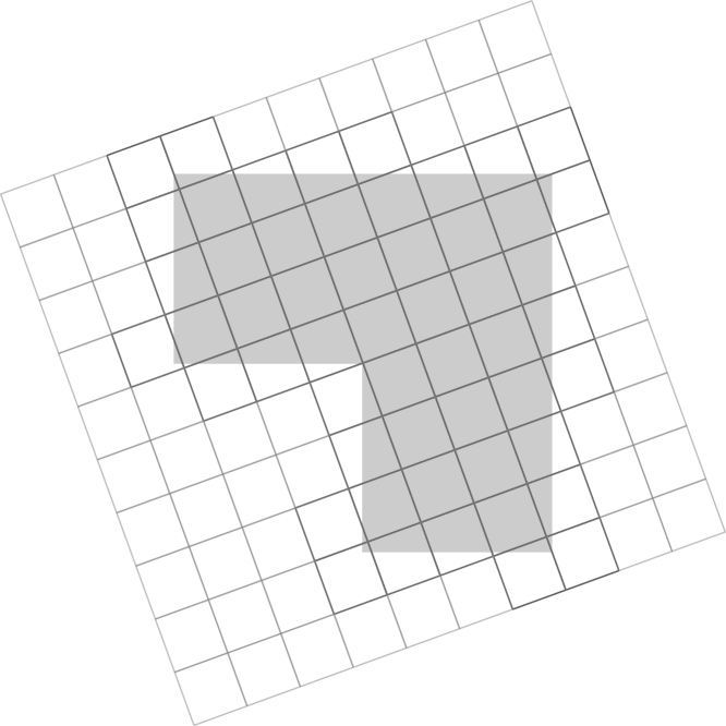
(a) Initial mesh

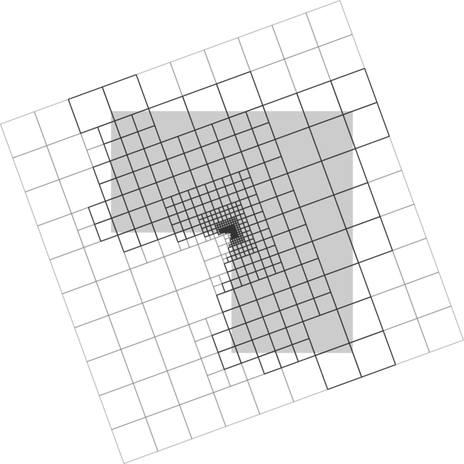
(b) Step $5$

Figure 11: Evolution of the mesh using the adaptive refinement procedure for the Stokes problem on a re-entrant corner domain using $k=2$.

Fig. 12 displays the error convergence results obtained using uniform and adaptive refinements, for both linear and quadratic THB-splines. The convergence rate when uniform refinements are considered is suboptimal, limited by the weak singularity at the re-entrant corner. Using adaptive mesh refinement results in a recovery of the optimal rates in the case of linear basis functions, with even higher rates observed for the quadratic splines on account of the highly-focused refinements resulting from the residual-based error estimator as observed in Fig. 11(b).

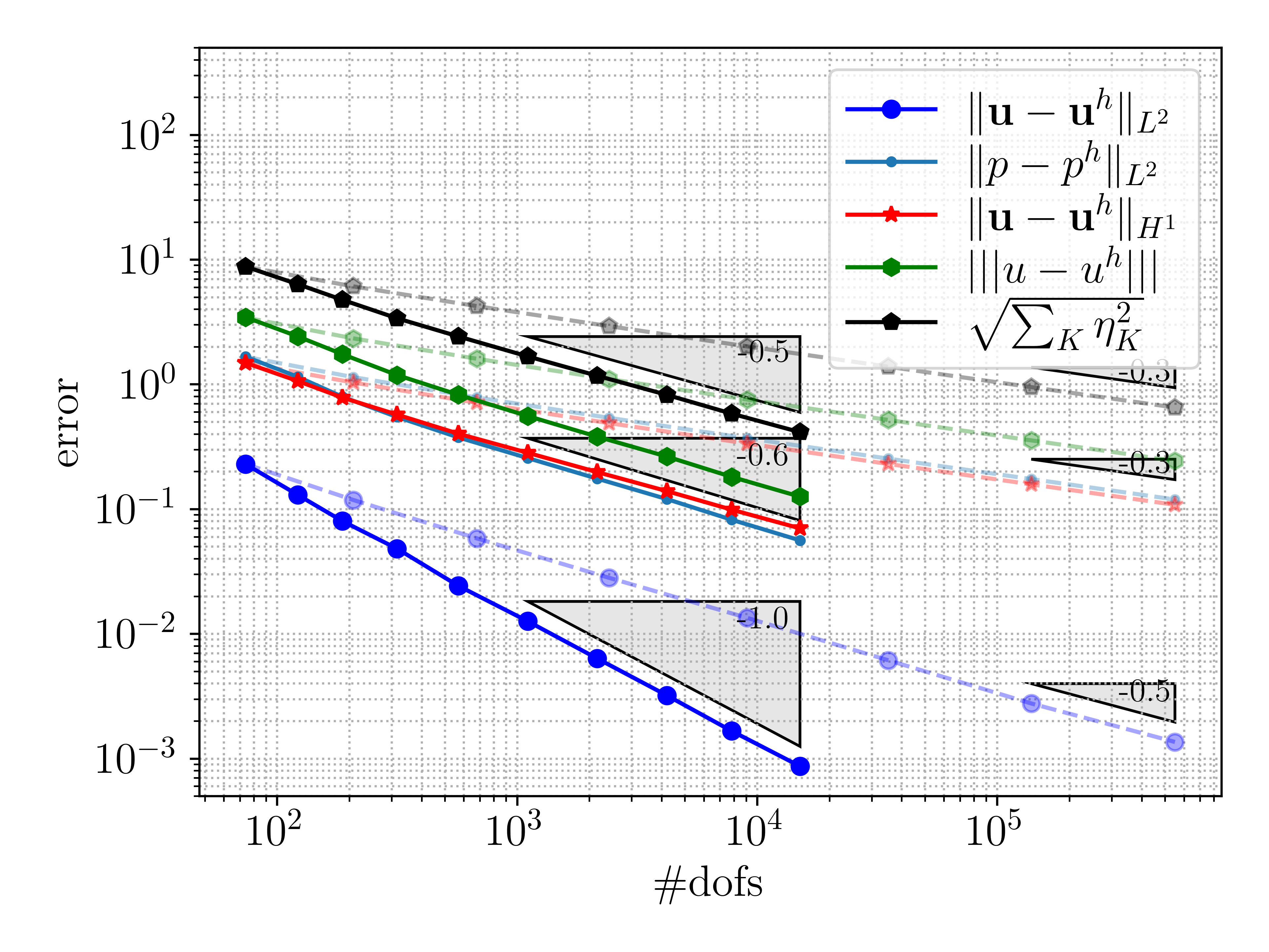
(a) $k=1$

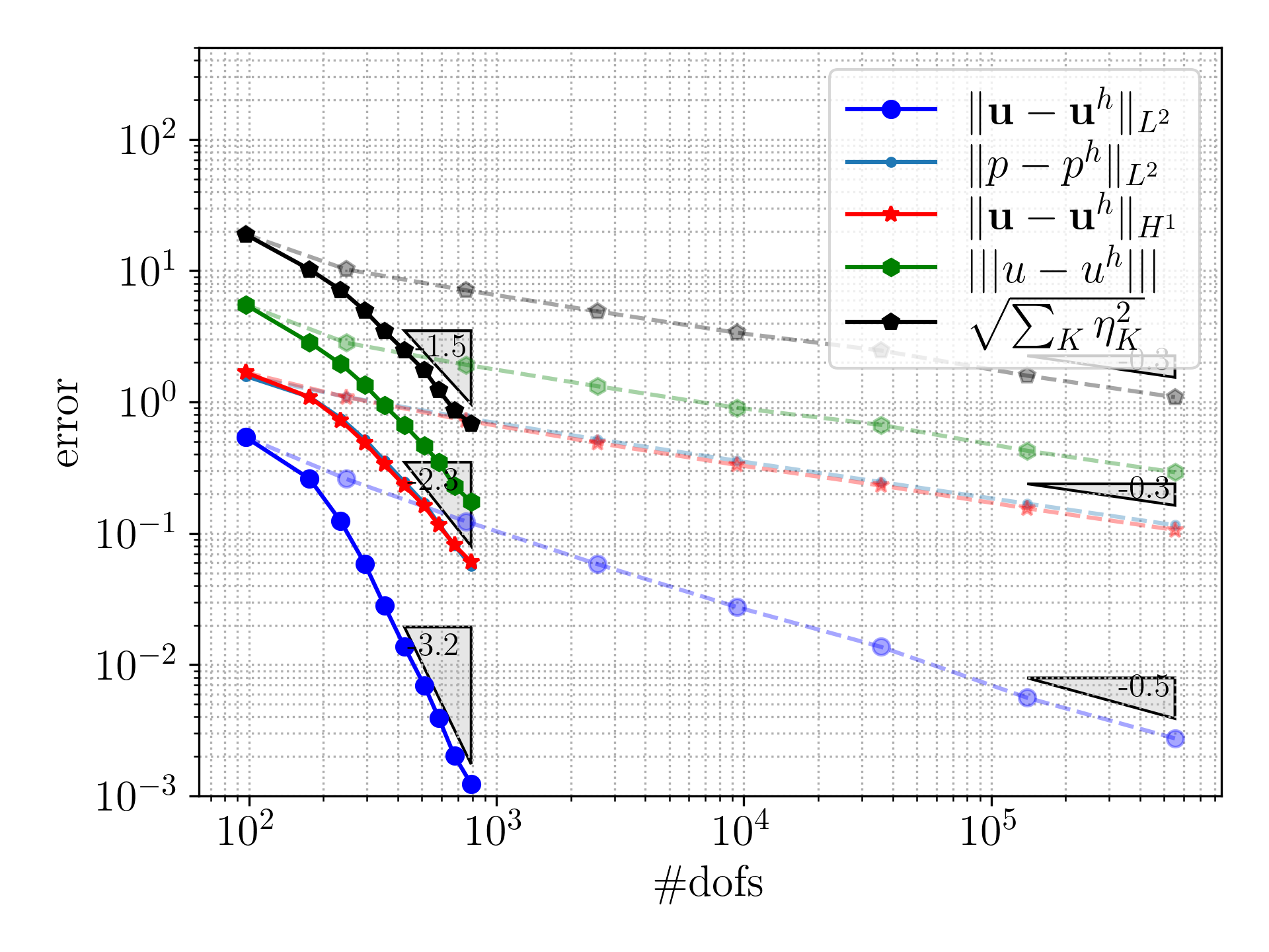
(b) $k=2$

Figure 12: Error convergence results for the Stokes problem on a re-entrant corner domain under residual-based adaptive refinement (solid) and uniform refinement (dashed) for linear ($k=1$) and quadratic ($k=2$) basis functions.

6 Scan-based flow simulations

To demonstrate the scan-based analysis workflow reviewed in this work, we consider the blood flow (viscosity $\mu=4\,{\rm mPa\cdot s}$) through the patient-specific ${\rm\mu CT}$-based carotid artery introduced in Section 2.3 (Fig. 7). Neumann conditions are imposed on the inflow (bottom) and outflow (top) boundaries, with the traction on the inflow boundary corresponding to a pressure of $17.3$ kPa ($130$ mmHg) and a zero-traction condition on the outflow boundary. Homogeneous Dirichlet conditions are imposed along the immersed boundaries to impose a no slip condition. The presented results are based on second-order ($k=2$) THB-splines. For details regarding the simulation setup we refer the reader to Ref. divi_residual-based_2022 (36), from which the results presented here are reproduced.

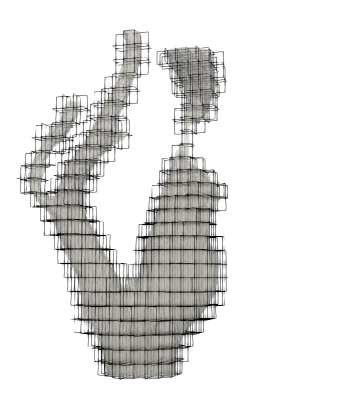
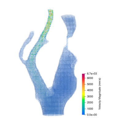
(a) Initial mesh with $3158$ #DOFs

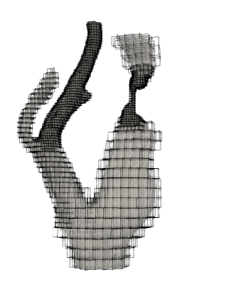
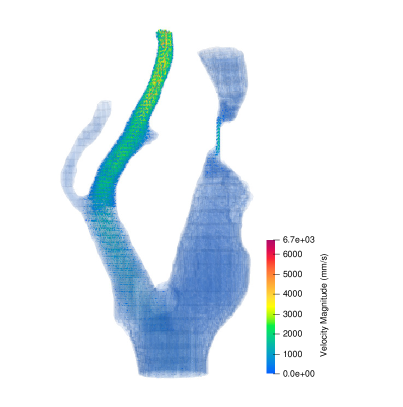
(b) Step $3$ with $12467$ #DOFs

Figure 13: Initial (13(a)) and final (13(b)) mesh (left) and velocity magnitude (right) for the patient-specific flow problem.

We consider an initial scan-domain mesh consisting of $24\times 24\times 24$ elements, with a scan size of $25.6\times 21.1\times 32.0\,{\rm mm}^{3}$. The octree depth is set to three. In this setting, after two refinements, an element is of a similar size as the voxels. The need to substantially refine beyond the voxel size is, from a practical perspective, questionable, as the dominant error in the analysis will then be related to the scan resolution and the segmentation procedure. In this sense, the constraint of not being able to refine beyond the octree depth is not a crucial problem in the considered simulations.

The initial mesh and final refinement result are shown in Fig. 13. The adaptive refinement procedure focuses on the regions where the errors are largest, i.e., near the stenosed section (i.e., the narrow region at the right artery) and at the outflow section of the left artery, such that important details of the solution are resolved. After the final refinement step, the adaptive simulation uses $12,816$ DOFs, which is substantially lower than the approximately $100,000$ DOFs that would have resulted from uniform mesh refinements up to the same level divi_topology-preserving_2022 (33).

7 Concluding remarks

In this contribution, we have reviewed the four key research contributions of our team with respect to scan-based immersed isogeometric flow analysis, viz.: (i) A spline-based image segmentation procedure, encompassing a voxel-data smoothing procedure, an octree-based procedure to obtain an explicit parametrization of the computational domain and its (immersed) boundary, and a topology-preservation strategy to restore smoothing-induced anomalies; (ii) A stabilized immersed formulation for (a.o.) Stokes flow, which ensures robustness with respect to unfavorably cut elements and enables the consideration of equal-order velocity-pressure discretizations without the loss of inf-sup stability; (iii) An adaptive procedure to optimize the distribution of integration points over cut elements, based on Strang’s first lemma; (iv) A mesh refinement procedure based on rigorous residual-based error estimates to refine the computational mesh in places where this results in significant accuracy improvements.

An important aspect of immersed (finite element) methods is the ill-conditioning associated with small (i.e., with a small volume fraction) or unfavorably cut (e.g., sliver-like) elements. Although not reviewed in this work, over the past decade our team has contributed to solving the challenges associated with ill-conditioning. The origin of the ill-conditioning problem was studied in detail by De Prenter et al. de_prenter_condition_2017 (44), which led to a scaling relation for the condition number with the smallest cut-element volume fraction. Dedicated preconditioning techniques, to be used in conjunction with iterative solvers, were developed based on the insights from this work, e.g., Refs. de_prenter_condition_2017 (44, 45, 27). We consider these (preconditioned) solver developments an important step in unlocking the potential of high-performance computing for immersed finite element methods jomo_robust_2019 (30). Note that the ghost- and skeleton-stabilization terms employed in the formulation in this chapter, which are primarily added to ensure well-posedness of the weak form, also resolve the conditioning problems, such that preconditioning techniques are not essential in this work.

The innovations in computational procedures and problem formulations yield a highly robust immersed isogeometric analysis workflow for scan-based analyses. Error-controlled simulations can be performed directly based on scan data, without the need for extensive user interactions. The effectivity of the framework is not fundamentally affected by the geometric and topological complexity of the scan data, on account of the decoupling of the geometry and computational mesh in immersed methods. The robustness of the framework derives from the rigorous mathematical underpinning of the considered methods.

Further developments to the scan-based workflow are required to enable the consideration of more advanced problems/formulations, such as higher Reynolds number flows (requiring additional stabilization), fluid-structure interactions and complex fluid models. Further improvements are also required to enhance the computational performance of the developed workflow. This mainly pertains to algorithm and code optimization, which is required to apply the developed workflow to, e.g., larger scans, time-dependent problems and non-linear problems. Detailed recommendations for specific further developments can be found in our referenced work; see Ref. divi_scan-based_2022 (64) for a summary of these.

- (1) Yongjie Zhang “Challenges and Advances in Image-Based Geometric Modeling and Mesh Generation” In Image-Based Geometric Modeling and Mesh Generation, Lecture Notes in Computational Vision and Biomechanics Dordrecht: Springer Netherlands, 2013, pp. 1–10 DOI: 10.1007/978-94-007-4255-0˙1
- (2) Thomas J.. Hughes et al. “Isogeometric analysis: CAD, finite elements, NURBS, exact geometry and mesh refinement” In Computer Methods in Applied Mechanics and Engineering 194.39, 2005, pp. 4135–4195 DOI: 10.1016/j.cma.2004.10.008
- (3) David F. Rogers “An introduction to NURBS: with historical perspective”, The Morgan Kaufmann Series in Computer Graphics San Francisco: Morgan Kaufmann Publishers, 2001 URL: http://site.ebrary.com/id/10190970
- (4) J. Cottrell et al. “Isogeometric Analysis: Toward Integration of CAD and FEA” John Wiley & Sons, 2009
- (5) J. Cottrell et al. “Isogeometric analysis of structural vibrations” In Computer Methods in Applied Mechanics and Engineering 195.41, John H. Argyris Memorial Issue. Part II, 2006, pp. 5257–5296 DOI: 10.1016/j.cma.2005.09.027
- (6) Yongjie Zhang et al. “Patient-specific vascular NURBS modeling for isogeometric analysis of blood flow” In Computer Methods in Applied Mechanics and Engineering 196.29, 2007, pp. 2943–2959 DOI: 10.1016/j.cma.2007.02.009
- (7) Martin Ruess et al. “Weak coupling for isogeometric analysis of non-matching and trimmed multi-patch geometries” In Computer Methods in Applied Mechanics and Engineering 269, 2014, pp. 46–71 DOI: 10.1016/j.cma.2013.10.009
- (8) Yuxuan Yu et al. “Anatomically realistic lumen motion representation in patient-specific space–time isogeometric flow analysis of coronary arteries with time-dependent medical-image data” In Computational Mechanics 65.2, 2020, pp. 395–404 DOI: 10.1007/s00466-019-01774-4
- (9) Thomas J.. Hughes et al. “Chapter 8 - Smooth multi-patch discretizations in Isogeometric Analysis” In Handbook of Numerical Analysis 22, Geometric Partial Differential Equations - Part II Elsevier, 2021, pp. 467–543 DOI: 10.1016/bs.hna.2020.09.002
- (10) Michele Bucelli et al. “Multipatch Isogeometric Analysis for electrophysiology: Simulation in a human heart” In Computer Methods in Applied Mechanics and Engineering 376, 2021, pp. 113666 DOI: 10.1016/j.cma.2021.113666
- (11) Yongjie Zhang et al. “Solid T-spline construction from boundary representations for genus-zero geometry” In Computer Methods in Applied Mechanics and Engineering 249-252, Higher Order Finite Element and Isogeometric Methods, 2012, pp. 185–197 DOI: 10.1016/j.cma.2012.01.014
- (12) Ming-Chen Hsu et al. “An interactive geometry modeling and parametric design platform for isogeometric analysis” In Computers & Mathematics with Applications 70.7, High-Order Finite Element and Isogeometric Methods, 2015, pp. 1481–1500 DOI: 10.1016/j.camwa.2015.04.002
- (13) Benjamin Urick et al. “Review of Patient-Specific Vascular Modeling: Template-Based Isogeometric Framework and the Case for CAD” In Archives of Computational Methods in Engineering 26.2, 2019, pp. 381–404 DOI: 10.1007/s11831-017-9246-z
- (14) Jamshid Parvizian et al. “Finite cell method: h- and p-extension for embedded domain problems in solid mechanics” In Computational Mechanics 41.1, 2007, pp. 121–133 DOI: 10.1007/s00466-007-0173-y
- (15) Alexander Düster et al. “The finite cell method for three-dimensional problems of solid mechanics” In Computer Methods in Applied Mechanics and Engineering 197.45, 2008, pp. 3768–3782 DOI: 10.1016/j.cma.2008.02.036
- (16) Dominik Schillinger and Martin Ruess “The Finite Cell Method: A Review in the Context of Higher-Order Structural Analysis of CAD and Image-Based Geometric Models” In Archives of Computational Methods in Engineering 22.3, 2015, pp. 391–455 DOI: 10.1007/s11831-014-9115-y
- (17) Erik Burman “Ghost penalty” In Comptes Rendus Mathematique 348.21, 2010, pp. 1217–1220 DOI: 10.1016/j.crma.2010.10.006
- (18) Erik Burman and Peter Hansbo “Fictitious domain finite element methods using cut elements: II. A stabilized Nitsche method” In Applied Numerical Mathematics 62.4, Third Chilean Workshop on Numerical Analysis of Partial Differential Equations, 2012, pp. 328–341 DOI: 10.1016/j.apnum.2011.01.008
- (19) Erik Burman et al. “CutFEM: Discretizing geometry and partial differential equations” In International Journal for Numerical Methods in Engineering 104.7, 2015, pp. 472–501 DOI: 10.1002/nme.4823
- (20) Ernst Rank et al. “Geometric modeling, isogeometric analysis and the finite cell method” In Computer Methods in Applied Mechanics and Engineering 249-252, Higher Order Finite Element and Isogeometric Methods, 2012, pp. 104–115 DOI: 10.1016/j.cma.2012.05.022
- (21) Dominik Schillinger et al. “An isogeometric design-through-analysis methodology based on adaptive hierarchical refinement of NURBS, immersed boundary methods, and T-spline CAD surfaces” In Computer Methods in Applied Mechanics and Engineering 249-252, Higher Order Finite Element and Isogeometric Methods, 2012, pp. 116–150 DOI: 10.1016/j.cma.2012.03.017
- (22) Martin Ruess et al. “Weakly enforced essential boundary conditions for NURBS-embedded and trimmed NURBS geometries on the basis of the finite cell method” In International Journal for Numerical Methods in Engineering 95.10, 2013, pp. 811–846 DOI: 10.1002/nme.4522
- (23) David Kamensky et al. “An immersogeometric variational framework for fluid–structure interaction: Application to bioprosthetic heart valves” In Computer Methods in Applied Mechanics and Engineering 284, Isogeometric Analysis Special Issue, 2015, pp. 1005–1053 DOI: 10.1016/j.cma.2014.10.040
- (24) Ming-Chen Hsu et al. “Direct immersogeometric fluid flow analysis using B-rep CAD models” In Computer Aided Geometric Design 43, Geometric Modeling and Processing 2016, 2016, pp. 143–158 DOI: 10.1016/j.cagd.2016.02.007
- (25) Clemens V. Verhoosel et al. “Image-based goal-oriented adaptive isogeometric analysis with application to the micro-mechanical modeling of trabecular bone” In Computer Methods in Applied Mechanics and Engineering 284, Isogeometric Analysis Special Issue, 2015, pp. 138–164 DOI: 10.1016/j.cma.2014.07.009
- (26) Martin Ruess et al. “The finite cell method for bone simulations: verification and validation” In Biomechanics and Modeling in Mechanobiology 11.3, 2012, pp. 425–437 DOI: 10.1007/s10237-011-0322-2
- (27) Frits Prenter et al. “Multigrid solvers for immersed finite element methods and immersed isogeometric analysis” In Computational Mechanics 65.3, 2020, pp. 807–838 DOI: 10.1007/s00466-019-01796-y
- (28) Tuong Hoang et al. “Skeleton-stabilized immersogeometric analysis for incompressible viscous flow problems” In Computer Methods in Applied Mechanics and Engineering 344, 2019, pp. 421–450 DOI: 10.1016/j.cma.2018.10.015
- (29) Alexander Düster et al. “Numerical homogenization of heterogeneous and cellular materials utilizing the finite cell method” In Computational Mechanics 50.4, 2012, pp. 413–431 DOI: 10.1007/s00466-012-0681-2
- (30) John N. Jomo et al. “Robust and parallel scalable iterative solutions for large-scale finite cell analyses” In Finite Elements in Analysis and Design 163, 2019, pp. 14–30 DOI: 10.1016/j.finel.2019.01.009
- (31) Massimo Carraturo et al. “Modeling and experimental validation of an immersed thermo-mechanical part-scale analysis for laser powder bed fusion processes” In Additive Manufacturing 36, 2020, pp. 101498 DOI: 10.1016/j.addma.2020.101498
- (32) Sai C. Divi et al. “Error-estimate-based adaptive integration for immersed isogeometric analysis” In Computers & Mathematics with Applications 80.11, High-Order Finite Element and Isogeometric Methods 2019, 2020, pp. 2481–2516 DOI: 10.1016/j.camwa.2020.03.026
- (33) Sai C. Divi et al. “Topology-preserving scan-based immersed isogeometric analysis” In Computer Methods in Applied Mechanics and Engineering 392, 2022, pp. 114648 DOI: 10.1016/j.cma.2022.114648
- (34) Tuong Hoang et al. “Mixed Isogeometric Finite Cell Methods for the Stokes problem” In Computer Methods in Applied Mechanics and Engineering 316, Special Issue on Isogeometric Analysis: Progress and Challenges, 2017, pp. 400–423 DOI: 10.1016/j.cma.2016.07.027
- (35) Gilbert Strang and George Fix “An Analysis of the Finite Element Method” Wellesley-Cambridge Press, 2008
- (36) Sai Chandana Divi et al. “Residual-based error estimation and adaptivity for stabilized immersed isogeometric analysis using truncated hierarchical B-splines” In Journal of Mechanics 38, 2022, pp. 204–237 DOI: 10.1093/jom/ufac015
- (37) Carlotta Giannelli et al. “THB-splines: The truncated basis for hierarchical splines” In Computer Aided Geometric Design 29.7, Geometric Modeling and Processing 2012, 2012, pp. 485–498 DOI: 10.1016/j.cagd.2012.03.025
- (38) Yuri Bazilevs et al. “Isogeometric analysis: approximation, stability and error estimates for h-refined meshes” Publisher: World Scientific Publishing Co. In Mathematical Models and Methods in Applied Sciences 16.7, 2006, pp. 1031–1090 DOI: 10.1142/S0218202506001455
- (39) Guang Deng and L.W. Cahill “An adaptive Gaussian filter for noise reduction and edge detection” In 1993 IEEE Conference Record Nuclear Science Symposium and Medical Imaging Conference, 1993, pp. 1615–1619 vol.3 DOI: 10.1109/NSSMIC.1993.373563
- (40) Michael Unser et al. “On the Asymptotic Convergence of B-spline Wavelets to Gabor Functions” In IEEE Transactions on Information Theory 38.2, 1992, pp. 864–872 DOI: 10.1109/18.119742
- (41) Vasco Varduhn et al. “The tetrahedral finite cell method: Higher-order immersogeometric analysis on adaptive non-boundary-fitted meshes” In International Journal for Numerical Methods in Engineering 107.12, 2016, pp. 1054–1079 DOI: 10.1002/nme.5207
- (42) Boris Delaunay “Sur la sphere vide” In Izv. Akad. Nauk SSSR, Otdelenie Matematicheskii i Estestvennyka Nauk 7.793, 1934, pp. 1–2
- (43) Mark Berg et al. “Computational geometry algorithms and applications” Spinger, 2008
- (44) Frits Prenter et al. “Condition number analysis and preconditioning of the finite cell method” In Computer Methods in Applied Mechanics and Engineering 316, Special Issue on Isogeometric Analysis: Progress and Challenges, 2017, pp. 297–327 DOI: 10.1016/j.cma.2016.07.006
- (45) Frits Prenter et al. “Preconditioning immersed isogeometric finite element methods with application to flow problems” In Computer Methods in Applied Mechanics and Engineering 348, 2019, pp. 604–631 DOI: 10.1016/j.cma.2019.01.030
- (46) Anita Hansbo and Peter Hansbo “An unfitted finite element method, based on Nitsche’s method, for elliptic interface problems” In Computer Methods in Applied Mechanics and Engineering 191.47, 2002, pp. 5537–5552 DOI: 10.1016/S0045-7825(02)00524-8
- (47) Anand Embar et al. “Imposing Dirichlet boundary conditions with Nitsche’s method and spline-based finite elements” In International Journal for Numerical Methods in Engineering 83.7, 2010, pp. 877–898 DOI: 10.1002/nme.2863
- (48) Frits Prenter et al. “A note on the stability parameter in Nitsche’s method for unfitted boundary value problems” In Computers & Mathematics with Applications 75.12, 2018, pp. 4322–4336 DOI: 10.1016/j.camwa.2018.03.032
- (49) Frits Prenter et al. “Stability and conditioning of immersed finite element methods: analysis and remedies” arXiv, 2022 DOI: 10.48550/arXiv.2208.08538
- (50) E. Brummelen et al. “An adaptive isogeometric analysis approach to elasto-capillary fluid-solid interaction” In International Journal for Numerical Methods in Engineering 122.19, 2021, pp. 5331–5352 DOI: 10.1002/nme.6388
- (51) Santiago Badia et al. “Mixed Aggregated Finite Element Methods for the Unfitted Discretization of the Stokes Problem” Publisher: Society for Industrial and Applied Mathematics In SIAM Journal on Scientific Computing 40.6, 2018, pp. B1541–B1576 DOI: 10.1137/18M1185624
- (52) Santiago Badia et al. “Linking ghost penalty and aggregated unfitted methods” In Computer Methods in Applied Mechanics and Engineering 388, 2022, pp. 114232 DOI: 10.1016/j.cma.2021.114232
- (53) Erik Burman and Peter Hansbo “Edge stabilization for the generalized Stokes problem: A continuous interior penalty method” In Computer Methods in Applied Mechanics and Engineering 195.19, 2006, pp. 2393–2410 DOI: 10.1016/j.cma.2005.05.009
- (54) Alireza Abedian et al. “Performance of different integration schemes in facing discontinuities in the finite cell method” Publisher: World Scientific In International Journal of Computational Methods 10.3, 2013, pp. 1350002
- (55) Alireza Abedian et al. “The finite cell method for the J2 flow theory of plasticity” In Finite Elements in Analysis and Design 69, 2013, pp. 37–47 DOI: 10.1016/j.finel.2013.01.006
- (56) Alexandre Ern and Jean-Luc Guermond “Theory and Practice of Finite Elements: 159” New York: Springer, 2004
- (57) Alireza Abedian and Alexander Düster “Equivalent Legendre polynomials: Numerical integration of discontinuous functions in the finite element methods” In Computer Methods in Applied Mechanics and Engineering 343, 2019, pp. 690–720 DOI: 10.1016/j.cma.2018.08.002
- (58) Roland Becker et al. “A finite element method for domain decomposition with non-matching grids” Number: 2 Publisher: EDP Sciences In ESAIM: Mathematical Modelling and Numerical Analysis 37.2, 2003, pp. 209–225 DOI: 10.1051/m2an:2003023
- (59) Mika Juntunen and Rolf Stenberg “Nitsche’s method for general boundary conditions” In Mathematics of computation 78.267, 2009, pp. 1353–1374
- (60) Franz Chouly et al. “Residual-based a posteriori error estimation for contact problems approximated by Nitsche’s method” In IMA Journal of Numerical Analysis 38.2, 2018, pp. 921–954 DOI: 10.1093/imanum/drx024
- (61) Willy Dörfler “A Convergent Adaptive Algorithm for Poisson’s Equation” Publisher: Society for Industrial and Applied Mathematics In SIAM Journal on Numerical Analysis 33.3, 1996, pp. 1106–1124 DOI: 10.1137/0733054
- (62) Göktürk Kuru et al. “Goal-adaptive Isogeometric Analysis with hierarchical splines” In Computer Methods in Applied Mechanics and Engineering 270, 2014, pp. 270–292 DOI: 10.1016/j.cma.2013.11.026
- (63) Rüdiger Verfürth “A review of a posteriori error estimation and adaptive mesh refinement techniques”, Advances in numerical mathematics Chichester; New York: Wiley-Teubner, 1996
- (64) Sai Chandana Divi “Scan-based immersed isogeometric analysis” ISBN: 9789038654690, 2022 URL: https://research.tue.nl/files/195948926/20220318_Divi_hf.pdf
- (65) Gertjan van Zwieten et al. “Nutils” Zenodo, 2022 DOI: 10.5281/zenodo.6006701