Listen2YourHeart: A Self-Supervised Approach for Detecting Murmur in Heart-Beat Sounds

Abstract

Heart murmurs are abnormal sounds present in heartbeats, caused by turbulent blood flow through the heart. The PhysioNet 2022 challenge targets automatic detection of murmur from audio recordings of the heart and automatic detection of normal vs. abnormal clinical outcome. The recordings are captured from multiple locations around the heart.

Our participation investigates the effectiveness of self-supervised learning for murmur detection. We train the layers of a backbone CNN in a self-supervised way with data from both this year’s and the 2016 challenge. We use two different augmentations on each training sample, and normalized temperature-scaled cross-entropy loss. We experiment with different augmentations to learn effective phonocardiogram representations. To build the final detectors we train two classification heads, one for each challenge task. We present evaluation results for all combinations of the available augmentations, and for our multiple-augmentation approach.

Our team’s, Listen2YourHeart, SSL murmur detection classifier received a weighted accuracy score of $0.737$ (ranked 13th out of 40 teams) and an outcome identification challenge cost score of $11946$ (ranked 7th out of 39 teams) on the hidden test set.

1 Introduction

Heart murmurs can be a sign of numerous serious heart conditions associated with increased mortality [1]. The development of accurate, non-invasive and easily accessible methods for heart murmur screening can help with prevention and/or timely treatment, especially for populations with reduced access to healthcare resources. The 2022 PhysioNet Challenge [2, 3] attempts to incentivize researchers towards developing methods for the automatic detection of abnormal heart waves or heart murmurs, by analyzing phonocardiogram (PCG) signals. The analysis of such auscultation signals can provide crucial information on the heart’s structure and potentially assist clinicians in early screenings or assessments. We propose tackling the challenge through Self-Supervised Learning (SSL) with Deep Neural Networks (DNN) for the classification of PCG signals.

Although DNNs have achieved remarkable success in various settings, they have not yet been able to establish themselves in clinical practice (including screening procedures). There are several reasons that may contribute to this. First of all, a false prediction may lead to serious consequences for the patient’s health or may incur unnecessary healthcare costs. Secondly, an already trained model may not maintain its performance on newly collected data [4]. An additional constraint is the fact that hospital and medical data may be weakly labeled, unlabeled and may be affected by exogenous noise.

All the above add up to a need for generalizable, adaptable and non-conventional model training methods. To this end, Self-Supervised Learning (SSL) techniques have been proposed for biosignal classification and have achieved promising results [5]. In SSL, the main idea is to learn invariant representations by transforming or augmenting the input data and by training a model to distinguish between representations originating from the same signal against those that come from different ones. In addition to medical image analysis [6], SSL methods have also been implemented for EEG [7] and ECG [8] signals. In this work, we explore the usage of contrastive SSL [9] for the classification of PCG signals. Specifically, we (i) propose employing SSL for the extraction of meaningful PCG signal representation, (ii) evaluate our method’s effectiveness with minimal fine-tuning on downstream tasks and (iii) explore promising combinations of augmentations for the PCG signal domain.

2 Materials and methods

The goal of the challenge [2, 3] is to classify a patient on two classification tasks: murmur detection and clinical outcome. For each patient there are one or more audio recordings available, taken from 5 different locations (one of the four valves or other).

Our approach is split in two steps, and is similar for each classification task. First, we train an audio-based classifier on windows of fixed length by directly propagating the patient label to the windows (the only exception is for the murmur class “present” where only windows from recording locations marked as “murmur locations” are labeled as “present”; windows from the rest recording locations are labeled as “absent”). Then, we predict a single label for the patient by first aggregating the window-level labels to recording-level labels and then the recording-level labels to a single patient-level label.

Our audio-based classifier is a convolutional neural network, based on the architecture of [10]. However, given the limited size of the dataset, we train the convolutional layers in a self-supervised way, based on the approach of [11]. Thus, we also use the dataset released for the 2016 challenge of PhysioNet [12] to extend our training dataset. It should be noted that the 2016 dataset does not contain labels that are relevant to the 2022 challenge.

The 2022 dataset contains audio at $4$ kHz while the 2016 dataset at $2$ kHz. Therefore, we choose to resample the 2022 dataset at $2$ kHz. We use windows of $5$ sec length with an overlap of $2.5$ sec. However, the first and last $2$ seconds of each recording are discarded as they might contain transient noise artifacts.

2.1 Self-supervised training

Each audio window $x$ is transformed into two versions, namely $x_{1}$ and $x_{2}$, by applying two different sets of augmentations. Specifically, we examine the following augmentations: cut-off filters (high-pass or low-pass, at $250$, $500$, and $750$ Hz), rewinding the signal, inverting (multiply by $-1$), random scaling (in the range of $0.5$ to $2.0$), adding zero-mean uniform noise and upsampling by a factor of $2$, while cropping symmetrically to maintain window size.

To train the $5$ convolutional layers of the $5$-sec input window architecture of [10] we project the output of the last convolutional layer on an $128$-D space (via a fully connected layer) and then minimize the normalized temperature-scaled cross-entropy loss [13]. For the cosine similarity with temperature [14], we use a temperature value of $0.1$ based on some initial experiments on the training set and on the findings of [11].

Batch size is set to $256$ (leading to $512$ after the two augmentations) and training is allowed for at most $50$ epochs (we use early stopping with a patience of $5$ epochs on a validation subset, more on Section 3.1). To train such a large batch we employ the LARS optimizer [15] with a linear warm-up of $5$ epochs to a learning rate of $0.1$ and then a cosine decay (with an alpha of $1\%$).

Once training concludes, the projection head is discarded, and the weights of the convolutional layers are frozen.

2.2 Murmur classification

Given a trained set of convolutional layers, we create a murmur classifier by appending a classification head of $3$ FC layers as in [11]. The last layer has $3$ neurons, one per murmur class (“present”, “unknown”, and “absent”) and uses softmax activation. We train only the FC layers using categorical cross-entropy loss and the Adam optimizer, with a learning rate of $10^{-4}$. Batch size is set to $64$ and we train for at most $200$ epochs using early stopping with $20$ epochs patience on a validation subset (more on Section 3.1).

Training yields a murmur classifier for audio windows. Given an audio recording, we follow the same procedure as in the training phase to extract windows and apply the trained murmur classifier on each window independently. We thus infer the probability of each murmur class for each window. These probabilities are aggregated for the entire recording by averaging across the windows (we have experimented with other aggregations but this method evidently seems to be the most effective). Ultimately, we characterize the entire recording with a single label, based on the most probable class.

To assign a “present” label to a patient, we require that at least one recording has been labeled “present”. If none of the recordings have been labeled as such and at least one recording has been labeled as “unknown” the patient inherits the “unknown” label. Finally, the “absent” label is assigned to the patient only if all of the recordings have been labeled accordingly.

2.3 Outcome classification

Training and inference for clinical outcome are very similar to murmur training and inference respectively. The only difference is that the classification problem is now binary (“abnormal” vs. “normal” clinical outcome). Window-level aggregations are performed again using averaging, and we require that at least one recording is classified as “abnormal” in order to label the patient’s clinical outcome as abnormal. If no such recording exists, we label the patient as “normal”.

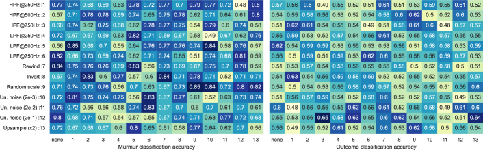
Figure 1: Augmentation comparison based on accuracy for murmur (left) and outcome (right) classification tasks.

3 Experiments and results

3.1 Experimental setup

The dataset provided by the challenge contains data from $942$ patients. We perform a stratified random split and keep $100$ patients as our test set, denoted $S_{\text{test}}$ (different from the hidden test set of the challenge). The remaining $842$ patients are again split (using a stratified random split) into a training set $S_{\text{train}}$ and a validation set $S_{\text{val}}$ ($80\%$-$20\%$). For SSL training, we also use the publically available 2016 challenge dataset [12, 16], which contains $3,541$ audio recordings, denoted $S_{\text{16}}$. We would like to note that $S_{\text{16}}$ does not contain labels relevant to this year’s challenge. Thus, SSL training is done on $S_{\text{16}}\cup S_{\text{train}}$, downstream training is done on $S_{\text{train}}$, and validation is always $S_{\text{val}}$. All results are reported on $S_{\text{test}}$.

3.2 Evaluation of augmentations

To adequately explore the most promising augmentations, we first evaluate each one of them separately (i.e. $x_{1}=f_{i}(x)$ and $x_{2}=x$ where $f_{i}$ are the different augmentations we examine) and subsequently in pairs (i.e. $x_{1}=f_{i}(x)$ and $x_{2}=f_{j}(x)$). Figure 1 summarizes the results for classification accuracy both for murmur and outcome labels.

For murmur classification and a single augmentation, the first column of Figure 1 shows that a low-pass filter at $250$ Hz, rewind, and uniform noise (of $0.02$ range) yield the best results (accuracy over $0.8$). The highest accuracy for pairs is $0.85$ and is obtained by two combinations: a high-pass filter at $500$ Hz with a high-pass filter at $250$ Hz, and random scaling with itself. Both of these pairs have the same or similar augmentations, however, and the resulting representations may not be informative. The following combinations of diverse augmentations achieve $0.84$ accuracy: invert with rewind, low-pass filter at $500$ Hz with uniform noise (range $0.002$), random scale with uniform noise (range $0.002$).

Accuracy for clinical outcome is generally lower. This is most probably due to the fact that, in clinical practice, decision for clinical outcome does not rely solely on listening to the audio recordings but also considers additional information such as the patient/examinee’s medical history (which were not taken into account in our case). The best results are obtained by combining uniform noise (range $0.01$) with either a high-pass filter at $750$ Hz, yielding $0.65$ accuracy, or with upsampling by $2$, yielding $0.64$ accuracy.

Table 1: Final results and baseline (fully supervised training on $S_{\text{train}}$).

	murmur			outcome
	F1-score	acc.	w. acc.	F1-score	acc.	w. acc.	cost
$f_{3}(f_{2}(f_{1}))$ vs. $g_{2}(g_{1})$	$0.544$	$0.590$	$0.668$	$0.657$	$0.590$	$0.764$	$10,541$
$f_{1}$ vs. $g_{2}(g_{1})$	$0.606$	$0.670$	$0.700$	$0.531$	$0.570$	$0.784$	$10,892$
$f_{3}(f_{2}(f_{1}))$ vs. $g_{1}$	$0.561$	$0.650$	$0.700$	$0.495$	$0.540$	$0.760$	$11,513$
Baseline	$0.524$	$0.600$	$0.558$	$0.515$	$0.550$	$0.750$	$11,276$

3.3 Challenge results

Based on these findings, we explore adding a second augmentation to one or both of the window copies. The final approach (that was submitted to the challenge) performs the following augmentations: the first copy of the window is high-pass filtered at $250$ Hz ($f_{1}$), followed by rewind with a $0.5$ probability ($f_{2}$), followed by inverting with a $0.5$ probability ($f_{3}$), while the second copy is polluted with uniform noise with a range of $0.02$ ($g_{1}$) followed by upsampling with a $0.5$ probability ($g_{2}$).

We present the results for this setup on the first row of Table 1, while also reporting the following additional metrics: F1-score, accuracy, and weighted accuracy. It should be noted that accuracy is weighed based on the challenge guidelines (for murmur: $\text{``present''}=5$, $\text{``unknown''}=3$, and $\text{``absent''}=1$, for outcome: $\text{``abnormal''}=5$ and $\text{``normal''}=1$). In the following two lines we present similar results where we omit one augmentation from each channel (rewind and inversion are removed together). Finally, the last line reports baseline results where no SSL is used at all, and the network is trained from top to bottom (no frozen weights) and individually for the murmur and outcome tasks, solely on the 2022 dataset.

The challenge is ranked based on murmur weighted accuracy and clinical outcome cost. Our models are able to surpass the fully supervised baseline and achieve a weighted accuracy of $0.668$ for murmur classification and a cost of $10,541$ for clinical outcome prediction. On the challenge’s hidden test set, we scored $0.737$ (Table 2) for murmur weighted accuracy and $11,946$ (Table 3) for outcome cost, achieving the 13th and 7th ranks respectively. Our results on the hidden test set suggest that our SSL-based model generalizes well to unseen data.

Training	Validation	Test	Ranking
0.786	0.671	0.737	13/40

Table 2: Weighted accuracy metric scores and ranking for our final selected entry (team Listen2YourHeart) for the murmur detection task.

Training	Validation	Test	Ranking
9720	10821	11946	7/39

Table 3: Cost metric scores and ranking, for our final selected entry (team Listen2YourHeart) for the clinical outcome identification task.

4 Conclusions

This work approaches the problem of PCG classification through SSL and evaluates its performance on the PhysioNet 2022 challenge. Results indicate that a backbone network trained via contrastive SSL improves performance compared to end-to-end supervised network training. By exploring and combining several augmentation techniques we are able to gain some intuition into which data transformations assist model training in this particular signal domain. Following this research, we aim to explore additional transformations and to introduce attention mechanisms into the model.

References

- [1] GBD 2017 Causes of Death Collaborators. Global, regional, and national age-sex-specific mortality for 282 causes of death in 195 countries and territories, 1980-2017: a systematic analysis for the Global Burden of Disease Study 2017. Lancet November 2018;392(10159):1736–1788. ISSN 1474-547X.
- [2] Reyna MA, Kiarashi Y, Elola A, Oliveira J, Renna F, Gu A, et al. Heart murmur detection from phonocardiogram recordings: The george b. moody physionet challenge 2022. medRxiv 2022;URL https://www.medrxiv.org/content/early/2022/08/16/2022.08.11.22278688.
- [3] Oliveira J, Renna F, Costa PD, Nogueira M, Oliveira C, Ferreira C, et al. The circor digiscope dataset: From murmur detection to murmur classification. IEEE Journal of Biomedical and Health Informatics 2022;26(6):2524–2535.
- [4] Ballas A, Diou C. A domain generalization approach for out-of-distribution 12-lead ecg classification with convolutional neural networks. In 2022 IEEE Eighth International Conference on Big Data Computing Service and Applications (BigDataService). 2022; 9–13.
- [5] Spathis D, Perez-Pozuelo I, Marques-Fernandez L, Mascolo C. Breaking away from labels: The promise of self-supervised machine learning in intelligent health. Patterns 2022;3(2):100410. ISSN 2666-3899.
- [6] Chen L, Bentley P, Mori K, Misawa K, Fujiwara M, Rueckert D. Self-supervised learning for medical image analysis using image context restoration. Medical Image Analysis 2019;58:101539. ISSN 1361-8415. URL https://www.sciencedirect.com/science/article/pii/S1361841518304699.
- [7] Gramfort A, Banville H, Chehab O, Hyvärinen A, Engemann D. Learning with self-supervision on eeg data. In 2021 9th International Winter Conference on Brain-Computer Interface (BCI). IEEE, 2021; 1–2.
- [8] Sarkar P, Etemad A. Self-supervised ecg representation learning for emotion recognition. IEEE Transactions on Affective Computing 2020;.
- [9] Jaiswal A, Babu AR, Zadeh MZ, Banerjee D, Makedon F. A survey on contrastive self-supervised learning. Technologies 2020;9(1):2.
- [10] Papapanagiotou V, Diou C, Delopoulos A. Chewing detection from an in-ear microphone using convolutional neural networks. In 2017 39th Annual International Conference of the IEEE Engineering in Medicine and Biology Society (EMBC). IEEE, 2017; 1258–1261.
- [11] Papapanagiotou V, Diou C, Delopoulos A. Self-supervised feature learning of 1d convolutional neural networks with contrastive loss for eating detection using an in-ear microphone. In 2021 43rd Annual International Conference of the IEEE Engineering in Medicine & Biology Society (EMBC). IEEE, 2021; 7186–7189.
- [12] Liu C, et al. An open access database for the evaluation of heart sound algorithms. Physiological Measurement nov 2016;37(12):2181–2213.
- [13] Oord Avd, Li Y, Vinyals O. Representation Learning with Contrastive Predictive Coding. arxiv180703748 csLG 2018;.
- [14] Hinton G, Vinyals O, Dean J, et al. Distilling the knowledge in a neural network. arXiv preprint arXiv150302531 2015;2(7).
- [15] You Y, Gitman I, Ginsburg B. Large Batch Training of Convolutional Networks. arXiv170803888 csCV 2017;.
- [16] Goldberger A, Amaral L, L. G, Hausdorff J, Ivanov PC, Mark R, et al. PhysioBank, PhysioToolkit, and PhysioNet: Components of a new research resource for complex physiologic signals., 2000.