Towards a multigrid method for the M₁ model for radiative transfer

Abstract

We present a geometric multigrid solver for the M₁ model of radiative transfer without source terms. In radiative hydrodynamics applications, the radiative transfer needs to be solved implicitly because of the fast propagation speed of photons relative to the fluid velocity. The M₁ model is hyperbolic and can be discretized with an HLL solver, whose time implicit integration can be done using a nonlinear Jacobi method. One can show that this iterative method always preserves the admissible states, such as positive radiative energy and reduced flux less than $1$. To decrease the number of iterations required for the solver to converge, and therefore to decrease the computational cost, we propose a geometric multigrid algorithm. Unfortunately, this method is not able to preserve the admissible states. In order to preserve the admissible state states, we introduce a pseudo-time such that the solution of the problem on the coarse grid is the steady state of a differential equation in pseudo-time. We present preliminary results showing the decrease of the number of iterations and computational cost as a function of the number of multigrid levels used in the method. These results suggest that nonlinear multigrid methods can be used as a robust implicit solver for hyperbolic systems such as the M₁ model.

1 Introduction

Radiative transfer describes the transport of radiation, it appears in a wide range of physical situations, from astrophysics, up to medicine. In radiation therapy, ionizing radiation can be used as a cancer treatment to control malignant cells (e.g., [1]). In astrophysical problems, the radiation exchanges energy with the surrounding gas. It is the domain of radiation hydrodynamics. Two phenomena have to be modeled: on one hand, the evolution of the fluid can be described by the Euler equations (e.g., [2]), on the other hand, the radiative transfer is described by an integro-differential equation [3, 4]. Some source terms model the energy exchange between the fluid and the radiation (e.g., [5]). In this work, we focus on the radiative transfer phenomenon, and we only consider completely transparent media, where the gas and radiation are not coupled. Photons are in a free-streaming regime, the medium is optically thin.

The quantity of interest for the radiative transfer is the specific intensity $I$. It depends on six variables: the time $t$, the position $\mathbf{{x}}$, the direction of propagation of the photons $\mathbf{{\Omega}}$, and the frequency of the photons $\nu$. Because of this high number of degrees of freedom, solving the integro-differential equation describing the radiative transfer while coupled with a grid-based code for hydrodynamics can be very costly. Several methods have been developed to tackle this issue, such as ray tracing (e.g., [6]) or Monte-Carlo methods (e.g., [7]). Ray tracing solves the problem by following the propagation of beams through the fluid. Although this method is very precise, it is highly costly when coupled with hydrodynamics codes. The number of degrees of freedom scales with the number of spatial cells multiplied by the number of radiation sources. Using a Monte-Carlo method, we follow the propagation of “photon energy packets” and their interactions with the fluid. It is based on a stochastic process, making this method accurate, but difficult to couple with a grid based hydrodynamics code. When the number of photon packets becomes too small in a region, a numerical noise can arise and pollute the simulation results.

In this work, we have chosen to use a gray moment model for the compromise between accuracy and low computational cost. The specific intensity is averaged over the direction of propagation and the frequency of the photons. One can consider the first two moments, the radiative energy $E_{\mathrm{r}}$ and the radiative flux $\mathbf{{F}}_{\mathrm{r}}$. A closure relation is needed to link the radiative flux to the radiative energy. A widely used model is the Flux-Limited Diffusion (FLD) approximation (e.g., [8]). However, this model can fail to capture the free-streaming regime of the photons in some cases, see e.g., [9]. One can consider an extra moment, the radiative pressure $\mathbb{P}_{\mathrm{r}}$. The closure relation expresses the radiative pressure as a function of radiative energy and radiative flux. We use the one given by the M₁ model ([10, 11]) for its good properties in both optically thin and optically thick media, where the radiation and the fluid strongly interact with each other, even though we do not consider this case.

An explicit solver for the radiative transfer would be restricted by a Courant-Friedrichs-Lewy (CFL) condition, limited by the speed of light. This will result in a very low time step compared to the hydrodynamics one, which is limited by the speed of sound of the fluid. We have chosen to use an implicit scheme to solve the M₁ model. The relation between the radiative energy, radiative flux, and radiative pressure is nonlinear, an implicit solver leads to a nonlinear system. It can be solved by using a Newton-Raphson method (e.g., [12]). At each iteration, a large sparse linear system has to be inverted. To obtain the best performances, preconditioned linear solvers have been developed, see for example the discussion in [13]. However, large time steps cannot be used in the free-streaming regime because, in general, the iterations of the Newton-Raphson method do not preserve the admissible states such as positive radiative energy and reduced flux less than $1$.

The M₁ model is a hyperbolic system with source terms. From a numerical point of view, the difficulty comes from a diffusion regime dictated by an asymptotic behavior. Numerous asymptotic preserving schemes that capture this asymptotic behavior have been developed. Some of them also preserve the admissible states but are explicit (e.g., [14, 15]), other schemes are implicit but encounter a reduced flux greater than $1$ especially in the free-streaming regime (e.g., [13]). In this work, we only consider the hyperbolic system, without source terms, and we present an implicit scheme that preserves the admissible states.

[16, 17] suggests solving the nonlinear system with a Jacobi method. Because this method is iterative, its convergence rate can be improved thanks to multigrid acceleration (e.g., [18, 19]). However, this algorithm is not specific to the radiative transfer problem and does not preserve the admissible states. Inspired by [20], we introduce a pseudo-time to tackle this issue.

This paper is organized as follows. We first present in more detail the M₁ model and its discretization in section 2. We then show in section 3 the Jacobi method to solve the nonlinear system arising from the discretization of the M₁ model. We explore the geometric multigrid technique in section 4 and we highlight the modification we made to apply it to radiative transfer. In section 5, we perform some tests to validate both algorithms. We also show some performance results. Finally, we reach our conclusion in section 6.

2 M₁ model and implicit discretization

2.1 Continuous model

The quantity of interest, the specific intensity $I$, describes the rate of radiative transfer of energy, at a point $\mathbf{{x}}$ and time $t$. It verifies the following equation:

$$\left(\frac{1}{c}\partial_{t}+\mathbf{{\Omega}}\cdot\nabla\right)I\left(\mathbf{{x}},t,\mathbf{{\Omega}},\nu\right) =-\left(\sigma^{\mathrm{a}}_{\nu}+\sigma^{\mathrm{s}}_{\nu}\right)I\left(\mathbf{{x}},t,\mathbf{{\Omega}},\nu\right)+\sigma^{\mathrm{a}}_{\nu}B\left(\nu,T_{\mathrm{g}}\right)$$ (1)

$$+\sigma^{\mathrm{s}}_{\nu}\int_{S^{2}}p^{\nu}\left(\mathbf{{\Omega}}\cdot\mathbf{{\Omega}}^{\prime}\right)I\left(\mathbf{{x}},t,\mathbf{{\Omega}}^{\prime},\nu\right)\mathrm{d}\Omega^{\prime},$$

where $c$ is the speed of light, $\nu$ is the frequency of the photons. $\mathbf{{\Omega}}$ is the direction of propagation of the photons: in the vacuum, photons propagate in a straight line at velocity $c\mathbf{{\Omega}}$. $\sigma^{\mathrm{a}}_{\nu}$ is the absorption coefficient, $\sigma^{\mathrm{s}}_{\nu}$ is the scattering coefficient, and $B$ is the black body specific intensity. See, for example, [3] for the derivation of eq. 1.

Let us now define the gray three first moments of the specific intensity as

$$E_{\mathrm{r}} =\frac{1}{c}\int_{0}^{\infty}\int_{S^{2}}I\left(\mathbf{{x}},t,\mathbf{{\Omega}},\nu\right)\mathrm{d}\Omega\mathrm{d}\nu$$ (2)

$$\mathbf{{F}}_{\mathrm{r}} =\int_{0}^{\infty}\int_{S^{2}}I\left(\mathbf{{x}},t,\mathbf{{\Omega}},\nu\right)\mathbf{{\Omega}}\mathrm{d}\Omega\mathrm{d}\nu$$

$$\mathbb{P}_{\mathrm{r}} =\frac{1}{c}\int_{0}^{\infty}\int_{S^{2}}I\left(\mathbf{{x}},t,\mathbf{{\Omega}},\nu\right)\mathbf{{\Omega}}\otimes\mathbf{{\Omega}}\mathrm{d}\Omega\mathrm{d}\nu.$$

$E_{\mathrm{r}}$ is the radiative energy, $\mathbf{{F}}_{\mathrm{r}}$ is the radiative flux, and $\mathbb{P}_{\mathrm{r}}$ is the radiative pressure.

Using eq. 1, one can show that the moments obey the following system:

$$\partial_{t}E_{\mathrm{r}}+\nabla\cdot\mathbf{{F}}_{\mathrm{r}} =c\left(\sigma_{\mathrm{P}}a_{\mathrm{r}}T_{\mathrm{g}}^{4}-\sigma_{\mathrm{E}}E_{\mathrm{r}}\right)$$ (3)

$$\partial_{t}\mathbf{{F}}_{\mathrm{r}}+c^{2}\nabla\cdot\mathbb{P}_{\mathrm{r}} =-c\left(\sigma_{\mathrm{F}}+\left(1-g\right)\sigma_{\mathrm{R}}\right)\mathbf{{F}}_{\mathrm{r}},$$

with $\sigma_{\mathrm{E}}$ (resp. $\sigma_{\mathrm{P}}$) the mean over frequency of $\sigma^{\mathrm{a}}_{\nu}$ weighted by the radiative energy (resp. the black body specific intensity), $\sigma_{\mathrm{F}}$ (resp. $\sigma_{\mathrm{S}}$) the mean of $\sigma^{\mathrm{a}}_{\nu}$ (resp. $\sigma^{\mathrm{s}}_{\nu}$) weighted by the radiative flux, $g$ the first moment of the phase function $p^{\nu}$, $T_{\mathrm{g}}$ the temperature of the gas, and $a_{\mathrm{r}}$ the radiative constant. See [9] for the discussion about the source terms and the approximations that can be made, such as $\sigma_{\mathrm{E}}=\sigma_{\mathrm{P}}$.

Using eq. 2, one can notice that $E_{\mathrm{r}}>0$ because $I>0$, and

$$\left\lvert\left\lvert\mathbf{{F}}_{\mathrm{r}}\right\lvert\right\lvert\leq\int_{0}^{\infty}\int_{S^{2}}\underbrace{I\left(\mathbf{{x}},t,\mathbf{{\Omega}},\nu\right)}_{\geq 0}\underbrace{\left\lvert\left\lvert\mathbf{{\Omega}}\right\lvert\right\lvert}_{=1}\mathrm{d}\Omega\mathrm{d}\nu=cE_{\mathrm{r}}.$$ (4)

This condition rewrites $f\leq 1$, where $f=\left\lvert\left\lvert\mathbf{{f}}\right\lvert\right\lvert=\frac{\left\lvert\left\lvert\mathbf{{\mathbf{{F}}_{\mathrm{r}}}}\right\lvert\right\lvert}{cE_{\mathrm{r}}}$ is the reduced flux. It ensures that the radiative energy cannot be transported faster than the speed of light. These two conditions, the positive radiative energy and the reduced flux less than $1$, have to be preserved by the numerical scheme, for physical and numerical reasons.

We now specify the closure relation, which is a way to express $\mathbb{P}_{\mathrm{r}}$ as a function of $E_{\mathrm{r}}$ and $\mathbf{{F}}_{\mathrm{r}}$. We have chosen to use the M₁ closure relation for its good properties in the free-streaming regime. We have

$$\mathbb{P}_{\mathrm{r}}=\left(\frac{1-\chi}{2}\mathbb{I}+\frac{3\chi-1}{2}\mathbf{{n}}\otimes\mathbf{{n}}\right)E_{\mathrm{r}},$$ (5)

where $\mathbf{{n}}=\frac{\mathbf{{f}}}{f}$ is a unit vector aligned with the reduced flux, $f=\left\lvert\left\lvert\mathbf{{f}}\right\lvert\right\lvert$, and $\mathbb{I}$ is the identity matrix. $\chi$ is the Eddington factor, defined as $\chi=\frac{3+4f^{2}}{5+2\sqrt{4-3f^{2}}}$. Equation 5 can be obtained by applying a Lorentz transform to an isotropic distribution of photons ([10]) or by maximizing the radiative entropy ([11]).

More details about the derivation of the model and the closure relation can be found in [21].

Developing numerical schemes to solve eq. 3 can be challenging due to the presence of the source terms and their behavior in optically thick media. Several numerical schemes that take into account the source terms have been developed, see e.g., [22, 23, 14]. However, most of them are explicit schemes. For some physical applications, an implicit scheme is mandatory. For example, in radiation hydrodynamics, when radiative transfer is coupled with hydrodynamics, the speed of light is larger than the speed of sound of the fluid. A solution to avoid a time step restricted by the speed of light for the hydrodynamics is to use an implicit solver for the radiative transfer. When both phenomena are coupled, source terms are mandatory to model this coupling. Developing an implicit scheme with source term is still an active topic of research. Here, we do not address the source terms, but we focus on the implicit property of the scheme In the following, we set $\sigma_{\mathrm{E}}=\sigma_{\mathrm{P}}=\sigma_{\mathrm{F}}=\sigma_{\mathrm{S}}=0$ which allows us to use standard numerical schemes for eq. 3.

One can show that the M₁ model is hyperbolic and can be written as

$$\partial_{t}\mathcal{U}+\nabla\cdot\mathcal{F}\left(\mathcal{U}\right)=0,$$

with $\mathcal{U}=\left(E_{\mathrm{r}},\mathbf{{\mathbf{{F}}_{\mathrm{r}}}}\right)$ and $\mathcal{F}$ the flux function, defined as $\mathcal{F}\left(\mathcal{U}\right)=\left(\mathbf{{\mathbf{{F}}_{\mathrm{r}}}},c^{2}\mathbb{P}_{\mathrm{r}}\right)$. The discretization of eq. 3 is discussed in the next section, without considering the source terms anymore.

2.2 HLL solver

Let us first introduce some notations. We note $h$ the step along the x-direction. $\Delta t$ is the time interval between the current time $t^{n}$ and $t^{n+1}$. We write $x_{i}$ the center of the cell $i$. We use the notation $u_{i}^{n}$ to represent the averaged quantity associated with the field $u$ at time $t^{n}$ in cell $i$ (finite volume). To ease notation, we drop the indices $\mathrm{r}$ for all radiative variables

The M₁ model is hyperbolic, we can discretize it using a time implicit HLL solver [24]. For the sake of simplicity, we only consider the one-dimensional case, but the extension to higher dimensions is straightforward. The flux at the interface $i+\frac{1}{2}$ between cells $i$ and $i+1$ depends on the speed of propagation, $\lambda_{i+\frac{1}{2}}^{+}$ and $\lambda_{i+\frac{1}{2}}^{-}$. $\lambda_{i+\frac{1}{2}}^{+}$ and $\lambda_{i+\frac{1}{2}}^{-}$ can be computed using the Eddington factor $\chi$. One can show that $\lambda_{i+\frac{1}{2}}^{+}\leq c$ and $\lambda_{i+\frac{1}{2}}^{-}\geq-c$. Using these upper bounds is sufficient for the scheme. Therefore, still for the sake of simplicity, we use these upper bounds in the flux. One can see the discussion in [9] about the impact of this choice. This is equivalent to use the Rusanov’s flux [25]. This leads to solving the following nonlinear system:

$$E^{n+1}_{i} \left(1+c\frac{\Delta t}{h}\right)-\frac{\Delta t}{2h}\left(cE^{n+1}_{i+1}-F^{n+1}_{i+1}\right)-\frac{\Delta t}{2h}\left(cE^{n+1}_{i-1}+F^{n+1}_{i-1}\right) =E^{n}_{i}$$ (6)

$$F^{n+1}_{i} \left(1+c\frac{\Delta t}{h}\right)-\frac{c\Delta t}{2h}\left(F^{n+1}_{i+1}-cP^{n+1}_{i+1}\right)-\frac{c\Delta t}{2h}\left(F^{n+1}_{i-1}+cP^{n+1}_{i-1}\right) =F^{n}_{i}.$$

Equation 6 can be solved using a Newton-Raphson method, as done in [13, 9] for example. However, numerical tests close to the free-streaming limit have shown that the admissible states are not preserved when large time steps are used. A solution is therefore to reduce the time step, but it leads to poor performances when the radiative transfer is coupled to hydrodynamics.

In the next section, we present another method to solve eq. 6 while preserving the admissible states.

3 Nonlinear Jacobi method

3.1 Algorithm

Let us follow the work of [16, 17]. We first define the set of admissible states

$$\mathcal{S}=\left\{\left(E_{\mathrm{r}},\mathbf{{F}}_{\mathrm{r}}\right),E_{\mathrm{r}}>0,\left\lvert\left\lvert\mathbf{{F}}_{\mathrm{r}}\right\lvert\right\lvert\leq cE_{\mathrm{r}}\right\}.$$ (7)

By writing $\mathbf{{v}}=\left(\cdots,E_{i},\mathbf{{F}}_{i},\cdots\right)^{T}\in\mathcal{S}^{N}$, where $N$ is the number of cells, eq. 6 rewrites

$$-\mathcal{L}^{h}\left(v^{n+1}_{i-1}\right)+\mathcal{D}^{h}\left(v^{n+1}_{i}\right)-\mathcal{R}^{h}\left(v^{n+1}_{i+1}\right)=v^{n}_{i},$$ (8)

where $v_{i}=\left(E_{i},\mathbf{{F}}_{i}\right)$. The operators $\mathcal{L}^{h}$, $\mathcal{D}^{h}$, and $\mathcal{R}^{h}$ contain the terms depending on $\left(E^{n+1}_{i-1},\mathbf{{F}}^{n+1}_{i-1}\right)$, $\left(E^{n+1}_{i},\mathbf{{F}}^{n+1}_{i}\right)$ and $\left(E^{n+1}_{i+1},\mathbf{{F}}^{n+1}_{i+1}\right)$ respectively. In 1D,

$$\mathcal{L}^{h}\left(v\right)=\begin{pmatrix}\frac{\Delta t}{2h}\left(cE+F\right)\\ \frac{c\Delta t}{2h}\left(F+cP\right)\end{pmatrix},\ \mathcal{D}^{h}\left(v\right)=\begin{pmatrix}\left(1+\frac{c\Delta t}{h}\right)E\\ \left(1+\frac{c\Delta t}{h}\right)F\end{pmatrix},\ \mathcal{R}^{h}\left(v\right)=\begin{pmatrix}\frac{\Delta t}{2h}\left(cE-F\right)\\ \frac{c\Delta t}{2h}\left(F-cP\right)\end{pmatrix}.$$ (9)

To ease notations, we write $\mathcal{L}=\mathcal{L}^{h}$, $\mathcal{D}=\mathcal{D}^{h}$, and $\mathcal{R}=\mathcal{R}^{h}$ when there is no ambiguity.

From [16], we solve eq. 8 using algorithm 1.

Algorithm 1 Nonlinear Jacobi method

1:Initialization: $\mathbf{{v}}^{n+1,(0)}=\mathbf{{v}}^{n}$

2:while $\left\lvert\left\lvert\mathcal{A}\left(\mathbf{{v}}^{n+1,(k)}\right)-\mathbf{{b}}\right\lvert\right\lvert>\varepsilon_{J}$ do

3:     for each cell $i$ do

4:         

$$v^{n+1,(k+1)}_{i}=\mathcal{D}^{-1}\left(b_{i}+\mathcal{L}\left(v^{n+1,(k)}_{i-1}\right)+\mathcal{R}\left(v^{n+1,(k)}_{i+1}\right)\right)$$ (10)

5:     end for

6:     $k\leftarrow k+1$

7:end while

8:$\mathbf{{v}}^{n+1}=\mathbf{{v}}^{n+1,(k)}$

Equation 6 can also be seen as

$$\mathcal{A}^{h}\left(\mathbf{{v}}\right)=\mathbf{{b}},$$ (11)

where $\mathcal{A}^{h}$ is a nonlinear operator, $\mathbf{{v}}$ is the vector of unknowns, and $\mathbf{{b}}$ is a known vector. As before, we drop the $h$ exponent whenever possible. The $i$-th row of $\mathcal{A}$ is

$$\left(\mathcal{A}\left(\mathbf{{v}}\right)\right)_{i}=\begin{pmatrix}E^{n+1}_{i}\left(1+c\frac{\Delta t}{h}\right)-\frac{\Delta t}{2h}\left(cE^{n+1}_{i+1}-F^{n+1}_{i+1}\right)-\frac{\Delta t}{2h}\left(cE^{n+1}_{i-1}+F^{n+1}_{i-1}\right)\\ F^{n+1}_{i}\left(1+c\frac{\Delta t}{h}\right)-\frac{c\Delta t}{2h}\left(F^{n+1}_{i+1}-cP^{n+1}_{i+1}\right)-\frac{c\Delta t}{2h}\left(F^{n+1}_{i-1}+cP^{n+1}_{i-1}\right)\end{pmatrix}.$$ (12)

Let us notice that if $\mathcal{A}$ is a linear operator, algorithm 1 simplifies into the classical Jacobi method for a tridiagonal matrix (see e.g., [26]).

It is shown in [16] that this algorithm converges to the unique solution $\mathbf{{v}}^{n+1}$ because the operator $\mathcal{A}$ is contractant. The proof relies on the study of the eigenvalues of the Jacobian of $\mathcal{A}$.

3.2 Preservation of the admissible states

Proposition 1.

If $v^{n}_{i}\in\mathcal{S}$, then $v^{n+1}_{i}$ obtained with algorithm 1 is also admissible, i.e., $v^{n+1}_{i}\in\mathcal{S}$.

Proof.

Let us show that if $\mathbf{{v}}^{n+1,(k)}\in\mathcal{S}^{N}$, then $\mathbf{{v}}^{n+1,(k+1)}\in\mathcal{S}^{N}$.

Let us recall Proposition 5.1 in [16]. We write it with our notations, but it can be used in a more general case. To fit [16]’s notations, we introduce $\mathbf{{m}}=\left(\frac{1}{c},\mathbf{{\Omega}}\right)$.

“Suppose $\mathcal{U}\in\mathcal{S}$ and the flux $\mathcal{F}\left(\mathcal{U}\right)$ is defined from a realizable closure, i.e. such that

$$\exists I>0\text{ s.t. }\mathcal{U}=\int_{0}^{\infty}\int_{S^{2}}\mathbf{{m}}I\mathrm{d}\Omega\mathrm{d}\nu,\ \mathcal{F}\left(\mathcal{U}\right)=\int_{0}^{\infty}\int_{S^{2}}c\mathbf{{\Omega}}\mathbf{{m}}I\mathrm{d}\Omega\mathrm{d}\nu,$$

then

$$\mathcal{U}\pm\mathcal{F}\left(\mathcal{U}\right)\in\mathcal{S}."$$

Furthermore, let us notice that the sum of two elements in $\mathcal{S}$ and the multiplication of an element of $\mathcal{S}$ by a positive scalar are also in $\mathcal{S}$ (but $\mathcal{S}$ is not a vector space because an element of $\mathcal{S}$ multiplied by a negative scalar is not in $\mathcal{S}$). One can then show that $\mathcal{L}$ and $\mathcal{R}$ are stable, i.e., $\mathcal{L}\left(v\right)\in\mathcal{S}$ and $\mathcal{R}\left(v\right)\in\mathcal{S}$ if $v\in\mathcal{S}$.

Therefore, because $b_{i}=v^{n}_{i}$, it is admissible and $b_{i}+\mathcal{L}\left(v_{i-1}\right)+\mathcal{R}\left(v_{i+1}\right)\in\mathcal{S}$.

Finally, in this particular case, $\mathcal{D}=\left(1+c\frac{\Delta t}{h}\right)\mathbb{I}$, where $\mathbb{I}$ is the identity matrix. So, if $v\in\mathcal{S}$, then $\mathcal{D}^{-1}\left(v\right)=\frac{1}{1+c\frac{\Delta t}{h}}v\in\mathcal{S}$.

We have shown that $\mathcal{D}^{-1}$, $\mathcal{L}$, and $\mathcal{R}$ are stable. Therefore, $v^{n+1,(k+1)}_{i}$ is admissible. By induction, the proof is complete.

∎

4 Geometric multigrid (GMG)

4.1 Convergence problematic

Figure 1: Evolution of the residual as a function of the number of iterations of Jacobi method, with different resolutions.

We investigate the performance of the nonlinear Jacobi algorithm on an academic test. The one considered here is the beam test described in [9, 27]. It is the propagation of a beam in the free-streaming regime. The domain is $[-1,1]\times[-1,1]$ and it is discretized with the same number of cells in the $x$ and $y$-directions. The initial temperature is $T_{0}=T_{\mathrm{r}}=$300\text{\,}\mathrm{K}$$, where $T_{\mathrm{r}}=\left(\frac{E_{\mathrm{r}}}{a_{\mathrm{r}}}\right)^{\frac{1}{4}}$ is the radiative temperature. The initial radiative flux is $\mathbf{{F}}_{\mathrm{r}}=\mathbf{{0}}$. At time $t=0$, a beam is introduced with $T_{\mathrm{r}}=$1~{}000\text{\,}\mathrm{K}$$ and $f=1$ with an angle of $45^{\circ}$ at $x=-1$ and $y\in[-0.875,-0.75]$. Because the solver is time-implicit, we set a time step $\Delta t$ such that the steady state is reached with one time iteration.

Number of cells	Cell-updates/$\mathrm{s}$
$129\times 129$	$146$
$257\times 257$	$76$
$513\times 513$	$38$

Table 1: Number of cell-updates per second of Jacobi method, with different resolutions.

Let us define the residual as

$$\mathbf{{r}}^{(k)}=\mathbf{{b}}-\mathcal{A}\left(\mathbf{{v}}^{(k)}\right).$$ (13)

Figure 1 shows the evolution of the norm of the residual as a function of the number of iterations of the Jacobi method, with different resolutions. If the operator $\mathcal{A}$ were linear, one could expect the residual to decrease linearly with the number of iterations, see, for example, results in [28] obtained with a linear problem. As the resolution increases, the number of iterations needed to reach the same residual also increases, from $4~{}000$ iterations with $129\times 129$ cells up to $15~{}000$ iterations with $513\times 513$ cells. As shown by table 1, performances decrease as the resolution increases, from around $150$ cell-updates/$\mathrm{s}$ with $129\times 129$ cells down to $40$ cell-updates/$\mathrm{s}$ with $513\times 513$ cells. If the number of iterations of the Jacobi method were constant with the resolution, the number of cell-updates/$\mathrm{s}$ would be constant. Because the method requires more iterations to reach the same residual when the resolution increases, performances decrease.

Indeed, [26] explains that the convergence rate decreases as the size of the problem increases, resulting in a decrease in performance. For linear problems, classical iterative methods are efficient to compute the high frequencies of the solution, but lack efficiency to compute its low frequencies. However, the computation is easier on a coarser grid with fewer unknowns. This observation has led to the development of the geometric multigrid (GMG) technique. The initial guess for the Jacobi algorithm (or any iterative method) is an interpolation of a solution computed on a coarser grid. This method requires information about the geometry of the problem, unlike preconditioners based on Krylov subspace. This additional information allows the multigrid method to be very efficient, but it lacks generality. To tackle this issue, algebraic multigrid methods have also been developed, see e.g., [26].

In this work, we focus on the GMG technique, and we first present the Full Approximation Scheme (FAS) in section 4.2 that can be used to solve a nonlinear system arising from the discretization of a differential equation. Then, in section 4.3 we apply it to the M₁ model, and we highlight the distinctive features of radiative transfer, i.e., the preservation of the admissible states $E_{\mathrm{r}}>0$ and $f\leq 1$.

4.2 General case

In this section, we present the main ideas of the geometric multigrid method. It does not intend to be a full review of existing work, see e.g., [18, 19].

We are interested in solving the nonlinear system eq. 11 with the Jacobi method presented in section 3. We assume that this system is obtained by the discretization of a differential equation on the domain $\Omega$ and therefore depends on a step $h$.

As mentioned above, the initial guess used in the Jacobi algorithm is the interpolation of a solution obtained on a coarser grid. This solution computed on the coarse grid can be itself computed thanks to a solution obtained on a third grid, even coarser. This process can be applied recursively until the last grid has only a few unknowns and the problem could be solved with a direct method, which leads to the so-called “nested iterations”. From [18], this requires the definition of two elements:

• a hierarchy of grids, completed with restriction and prolongation operators;

• an iterative method used as a smoother to solve the system on a given mesh.

In the linear case, one can study the eigenvalues and eigenvectors of $\mathcal{A}$, as well as the iterative method to understand how the smoother allows the quick decrease of the high frequencies of the error.

The hierarchy of grids is handled through recursiveness, we only need to describe the method with two grids. The domain $\Omega$ is discretized with two Cartesian meshes: the first one with step $h$, written $\Omega_{h}$ and the second one with step $2h$, written $\Omega_{2h}$. $\Omega_{h}$ contains $2^{d}$ times more elements than $\Omega_{2h}$, where $d$ is the dimension of the problem.

Each vector or operator is defined on a mesh. To highlight the dependence on the mesh, we write all the objects with the size of the grid it is defined on. For example, we write now $\mathbf{{v}}^{h}$ instead of $\mathbf{{v}}$.

Let us now define the restriction and prolongation operators used for inter-grid operations. We write the prolongation operator $\mathcal{P}_{2h}^{h}:\Omega_{2h}\rightarrow\Omega_{h}$ and the restriction operator $\mathcal{R}_{h}^{2h}:\Omega_{h}\rightarrow\Omega_{2h}$.

Figure 2: Prolongation operator in the one-dimensional case with weights. Ticks represent the interfaces between two cells, and the indices of the cells are located at the center. The blue arrow represents the operator if $i^{h}$ is even, and the red arrows represent the operator if $i^{h}$ is odd.

We use full weighting operators ([29]). Let us begin with the prolongation operator. Let us consider the one-dimensional case with an even number of cells in the fine mesh. Cells with index $i^{h}$ even in the fine mesh are the same as cells in the coarse mesh with index $i^{2h}$ (see fig. 2). Values corresponding to these cells in the coarse mesh are just moved in the fine mesh. The other values in the fine mesh are obtained by linear interpolation. The prolongation operator writes

$$\left(\mathcal{P}_{2h}^{h}\left(\mathbf{{v}}^{2h}\right)\right)_{i^{h}}=\left\{\begin{aligned} &\mathbf{{v}}^{2h}_{i^{2h}}\text{ if }i^{h}\text{ is even},\\ &\frac{1}{2}\left(\mathbf{{v}}^{2h}_{i^{2h}}+\mathbf{{v}}^{2h}_{i^{2h}+1}\right)\text{ if }i^{h}\text{ is odd}.\end{aligned}\right.$$ (14)

Figure 3: Prolongation operator in the two-dimensional case with weights. The blue arrow represents the operator if $i^{h}$ is even and $j^{h}$ is even. The red arrows represent the operator if $i^{h}$ is odd and $j^{h}$ is even. The green arrows represent the operator if $i^{h}$ is even and $j^{h}$ is odd. The orange arrows represent the operator if $i^{h}$ is odd and $j^{h}$ is odd.

We present now the prolongation operator in the two-dimensional case (see fig. 3). A cell $i^{h},j^{h}$ in the fine mesh $\Omega_{h}$ can be mapped directly into the cell $i^{2h},j^{2h}$ in the coarse mesh $\Omega_{2h}$, with $i^{h}=2i^{2h}$ and $j^{h}=2j^{2h}$. The value in a cell of the fine mesh is obtained by the interpolation in one direction, followed by the interpolation in the other direction. The interpolation in the $x$-direction gives

$$\left(\mathcal{P}_{2h}^{h}\left(\mathbf{{v}}^{2h}\right)\right)_{2i^{2h},2j^{2h}}=\mathbf{{v}}^{2h}_{i^{2h},j^{2h}}\text{ and }\left(\mathcal{P}_{2h}^{h}\left(\mathbf{{v}}^{2h}\right)\right)_{2i^{2h}+1,2j^{2h}}=\frac{1}{2}\left(\mathbf{{v}}^{2h}_{i^{2h},j^{2h}}+\mathbf{{v}}^{2h}_{i^{2h}+1,j^{2h}}\right).$$ (15)

The interpolation in the $y$-direction preserves these values and gives

$$\left(\mathcal{P}_{2h}^{h}\left(\mathbf{{v}}^{2h}\right)\right)_{2i^{2h},2j^{2h}+1}=\frac{1}{2}\left(\mathbf{{v}}^{2h}_{i^{2h},j^{2h}}+\mathbf{{v}}^{2h}_{i^{2h},j^{2h}+1}\right).$$ (16)

Finally, the last value is given by

$$\left(\mathcal{P}_{2h}^{h}\left(\mathbf{{v}}^{2h}\right)\right)_{2i^{2h}+1,2j^{2h}+1}=\frac{1}{4}\left(\mathbf{{v}}^{2h}_{i^{2h},j^{2h}}+\mathbf{{v}}^{2h}_{i+1^{2h},j^{2h}}+\mathbf{{v}}^{2h}_{i^{2h},j^{2h}+1}+\mathbf{{v}}^{2h}_{i^{2h}+1,j^{2h}+1}\right)$$ (17)

Using eqs. 15, 16 and 17 leads to writing the prolongation operator as

$$\left(\mathcal{P}_{2h}^{h}\left(\mathbf{{v}}^{2h}\right)\right)_{i^{h},j^{h}}=\left\{\begin{aligned} &\mathbf{{v}}^{2h}_{i^{2h},j^{2h}}\text{ if }i^{h}\text{ is even and }j^{h}\text{ is even},\\ &\frac{1}{2}\left(\mathbf{{v}}^{2h}_{i^{2h},j^{2h}}+\mathbf{{v}}^{2h}_{i^{2h}+1,j^{2h}}\right)\text{ if }i^{h}\text{ is odd and }j^{h}\text{ is even},\\ &\frac{1}{2}\left(\mathbf{{v}}^{2h}_{i^{2h},j^{2h}}+\mathbf{{v}}^{2h}_{i^{2h},j+1^{2h}}\right)\text{ if }i^{h}\text{ is even and }j^{h}\text{ is odd},\\ &\frac{1}{4}\left(\mathbf{{v}}^{2h}_{i^{2h},j^{2h}}+\mathbf{{v}}^{2h}_{i+1^{2h},j^{2h}}+\mathbf{{v}}^{2h}_{i^{2h},j^{2h}+1}+\mathbf{{v}}^{2h}_{i^{2h}+1,j^{2h}+1}\right)\\ &\quad\text{ if }i^{2h}\text{ is odd and }j^{2h}\text{ is odd}.\end{aligned}\right.$$ (18)

Let us now consider the restriction operator. We first consider the one-dimensional case, where the mesh is given by fig. 2. The prolongation operator can be made explicit, with appropriate boundary conditions:

$$\mathbf{{v}}^{h}=\left(\mathcal{P}_{2h}^{h}\left(\mathbf{{v}}^{2h}\right)\right)=\begin{pmatrix}\mathbf{{v}}^{h}_{1}\\ \mathbf{{v}}^{h}_{2}\\ \mathbf{{v}}^{h}_{3}\\ \mathbf{{v}}^{h}_{4}\\ \mathbf{{v}}^{h}_{5}\\ \mathbf{{v}}^{h}_{6}\\ \mathbf{{v}}^{h}_{7}\end{pmatrix}=\begin{pmatrix}\mathbf{{v}}^{h}_{2\times 0+1}\\ \mathbf{{v}}^{h}_{2\times 1}\\ \mathbf{{v}}^{h}_{2\times 1+1}\\ \mathbf{{v}}^{h}_{2\times 2}\\ \mathbf{{v}}^{h}_{2\times 2+1}\\ \mathbf{{v}}^{h}_{2\times 3}\\ \mathbf{{v}}^{h}_{2\times 3+1}\end{pmatrix}=\frac{1}{2}\begin{pmatrix}1&0&0\\ 2&0&0\\ 1&1&0\\ 0&2&0\\ 0&1&1\\ 0&0&2\\ 0&0&1\\ \end{pmatrix}\begin{pmatrix}\mathbf{{v}}^{2h}_{1}\\ \mathbf{{v}}^{2h}_{2}\\ \mathbf{{v}}^{2h}_{3}\end{pmatrix}.$$ (19)

Even though the prolongation operator is written as an operator, it is linear and can therefore be seen as a matrix, $\mathcal{P}_{2h}^{h}$. Apart from the first and the last rows that handle boundary conditions, the sum of the coefficients in a row is $1$. Values on the fine mesh are convex combinations of values on the coarse mesh.

We take the restriction operator as the transpose of the prolongation operator: $\mathcal{R}_{h}^{2h}=\frac{1}{2^{d}}\left(\mathcal{P}_{2h}^{h}\right)^{T}$, where $d$ is the dimension of the problem ($d\in\left\{1,2,3\right\}$). Thanks to the factor $\frac{1}{2^{d}}$, values on the coarse mesh are also convex combinations of values on the fine mesh. In the one-dimensional case given by fig. 2, the restriction operator writes

$$\mathbf{{v}}^{2h}=\left(\mathcal{R}_{h}^{2h}\left(\mathbf{{v}}^{2h}\right)\right)=\begin{pmatrix}\mathbf{{v}}^{2h}_{1}\\ \mathbf{{v}}^{2h}_{2}\\ \mathbf{{v}}^{2h}_{3}\end{pmatrix}=\frac{1}{4}\begin{pmatrix}1&2&1&0&0&0&0\\ 0&0&1&2&1&0&0\\ 0&0&0&0&1&2&1\\ \end{pmatrix}\begin{pmatrix}\mathbf{{v}}^{h}_{1}\\ \mathbf{{v}}^{h}_{2}\\ \mathbf{{v}}^{h}_{3}\\ \mathbf{{v}}^{h}_{4}\\ \mathbf{{v}}^{h}_{5}\\ \mathbf{{v}}^{h}_{6}\\ \mathbf{{v}}^{h}_{7}\end{pmatrix}.$$ (20)

In the general one-dimensional case, we have

$$\left(\mathcal{R}_{h}^{2h}\left(\mathbf{{v}}^{h}\right)\right)_{i^{2h}} =\frac{1}{4}\mathbf{{v}}^{h}_{i^{h}-1}+\frac{1}{2}\mathbf{{v}}^{h}_{i^{h}}+\frac{1}{4}\mathbf{{v}}^{h}_{i^{h}+1}.$$ (21)

Numerical tests in section 5 are done in the two-dimensional case, we also make $\mathcal{R}_{h}^{2h}$ explicit with $d=2$:

$$\left(\mathcal{R}_{h}^{2h}\left(\mathbf{{v}}^{h}\right)\right)_{i^{2h},j^{2h}} =\frac{1}{16}\mathbf{{v}}^{h}_{i^{h}-1,j^{h}-1}+\frac{1}{8}\mathbf{{v}}^{h}_{i^{h}-1,j^{h}}+\frac{1}{16}\mathbf{{v}}^{h}_{i^{h}-1,j^{h}+1}$$ (22)

$$+\frac{1}{8}\mathbf{{v}}^{h}_{i^{h},j^{h}-1}+\frac{1}{4}\mathbf{{v}}^{h}_{i^{h},j^{h}}+\frac{1}{8}\mathbf{{v}}^{h}_{i^{h},j^{h}+1}$$

$$+\frac{1}{16}\mathbf{{v}}^{h}_{i^{h}+1,j^{h}-1}+\frac{1}{8}\mathbf{{v}}^{h}_{i^{h}+1,j^{h}}+\frac{1}{16}\mathbf{{v}}^{h}_{i^{h}+1,j^{h}+1}.$$

Now that we have made explicit the restriction and prolongation operators used with two grids, we write the two-grid full approximation scheme.

Figure 4: Restriction of a smooth function.

One can show that the presence of smooth modes in the error between the approximate and exact solution can cause the relaxation to stall. In the linear case, the proof relies on the study of the eigenvalues and eigenvectors of $\mathcal{A}$, see e.g., [19] where the Poisson equation is solved. As shown by fig. 4, a smooth function on the fine mesh will be less smooth on the coarse mesh. An iterative method such as Jacobi will converge faster and will smooth the error on the coarse mesh. This gives the idea of restricting and prolonging the error between the different meshes. The function plotted in fig. 4 is a generic function to illustrate the interest of the restriction. It does not relate with our problem. If $\mathbf{{v}}$ is an approximate solution of eq. 11 and $\mathbf{{u}}$ is the exact solution, let us define the error as $\mathbf{{e}}=\mathbf{{u}}-\mathbf{{v}}$. By defining the residual $\mathbf{{r}}=\mathbf{{b}}-\mathcal{A}\mathbf{{v}}$ (eq. 13), the error verifies the following equation:

$$\mathbf{{r}} =\mathbf{{b}}-\mathcal{A}\left(\mathbf{{v}}\right)$$ (23)

$$=\mathcal{A}\left(\mathbf{{u}}\right)-\mathcal{A}\left(\mathbf{{v}}\right).$$

The error can be computed by solving the residual equation eq. 23 on the coarse mesh:

$$\mathcal{A}^{2h}\left(\mathbf{{u}}^{2h}\right)=\mathcal{A}^{2h}\left(\mathbf{{v}}^{2h}\right)+\mathbf{{r}}^{2h},$$ (24)

whose right-hand side is known. $\mathbf{{r}}^{2h}=\mathcal{R}_{h}^{2h}\left(\mathbf{{r}}^{h}\right)=\mathcal{R}_{h}^{2h}\left(\mathbf{{b}}^{h}-\mathcal{A}^{h}\left(\mathbf{{v}}^{h}\right)\right)$ is an approximation of the residual on the coarse mesh. Likewise, $\mathbf{{v}}^{2h}=\mathcal{R}_{h}^{2h}\left(\mathbf{{v}}^{h}\right)$. The new approximate solution on the fine mesh can be computed:

$$\mathbf{{v}}^{h}+\mathcal{P}_{2h}^{h}\left(\underbrace{\mathbf{{u}}^{2h}-\mathbf{{v}}^{2h}}_{\mathbf{{e}}^{2h}}\right).$$ (25)

The solution of the problem solved on the coarse mesh is the full approximation $\mathbf{{u}}^{2h}=\mathbf{{v}}^{2h}+\mathbf{{e}}^{2h}$, and not the error $\mathbf{{e}}^{2h}$. This leads to the full approximation scheme algorithm 2 ([18]).

One could try to solve $\mathcal{A}^{2h}\left(\mathbf{{v}}^{2h}\right)=\mathbf{{b}}^{2h}$ on the fine grid instead of solving eq. 24. However, numerical experiments show that solving eq. 24 and correcting the solution with eq. 25 is required to achieve convergence on the fine grid.

Algorithm 2 Two-grid full approximation scheme

1:Pre-smoother: relax $\nu_{0}$ times $\mathcal{A}^{h}\left(\mathbf{{u}}^{h}\right)=\mathbf{{b}}^{h}$ with initial guess $\mathbf{{v}}^{h}$ on the fine mesh $\Omega_{h}$

2:Restrict the residual $\mathbf{{r}}^{2h}=\mathcal{R}_{h}^{2h}\left(\mathbf{{b}}^{h}-\mathcal{A}^{h}\left(\mathbf{{u}}^{h}\right)\right)$ and the current solution $\mathbf{{v}}^{2h}=\mathcal{R}_{h}^{2h}\left(\mathbf{{u}}^{h}\right)$

3:Solve $\mathcal{A}^{2h}\left(\mathbf{{u}}^{2h}\right)=\mathbf{{r}}^{2h}+\mathcal{A}^{2h}\left(\mathbf{{v}}^{2h}\right)$ with initial guess $\mathbf{{v}}^{2h}$ on the coarse mesh $\Omega_{2h}$

4:Correct the approximation on the fine mesh: $\mathbf{{\bar{v}}}^{h}=\mathbf{{v}}^{h}+\mathcal{P}_{2h}^{h}\left(\mathbf{{u}}^{2h}-\mathbf{{v}}^{2h}\right)$

5:Post-smoother: relax $\nu_{0}$ times $\mathcal{A}^{h}\left(\mathbf{{u}}^{h}\right)=\mathbf{{b}}^{h}$ with initial guess $\mathbf{{\bar{v}}}^{h}$ on the fine mesh $\Omega_{h}$

If $\mathcal{A}$ were linear, we would have $\mathbf{{r}}=\mathcal{A}\left(\mathbf{{u}}\right)-\mathcal{A}\left(\mathbf{{v}}\right)=\mathcal{A}\left(\mathbf{{u}}-\mathbf{{v}}\right)=\mathcal{A}\left(\mathbf{{e}}\right)$. Instead of solving eq. 24 on the coarse mesh, we would solve

$$\mathcal{A}^{2h}\left(\mathbf{{e}}^{2h}\right)=\mathbf{{r}}^{2h},$$ (26)

and eq. 25 would be replaced by

$$\mathbf{{v}}^{h}+\mathcal{P}_{2h}^{h}\left(\mathbf{{e}}^{2h}\right).$$ (27)

Because $\mathcal{A}$ is nonlinear, we have to use the FAS algorithm.

This process can now be applied recursively until a mesh coarse enough is reached. This leads to the so-called V-cycle algorithm. Solving the nonlinear system at a given level is less costly than the previous level because the number of unknowns is reduced. However, numerical experiments have shown that the best performances are obtained by performing a series of V-cycles. In the linear case, a direct solver could be used at the coarsest level. In the case of radiative transfer, we will use the Jacobi method as a coarse grid solver.

4.3 Application to the HLL solver for the M₁ model

Let us now apply algorithm 2 to solve eq. 6. The operator $\mathcal{A}$ is the one described in section 3, and we use algorithm 1 as smoother and coarse grid solver. The system to be solved on the coarse mesh is

$$\mathcal{A}^{2h}\left(\mathbf{{u}}^{2h}\right)=\mathcal{A}^{2h}\left(\mathbf{{v}}^{2h}\right)+\mathbf{{r}}^{2h}.$$ (28)

As shown in section 3.2, if the initial guess for $\mathbf{{u}}^{2h}$ and the right-hand side $\mathcal{A}^{2h}\left(\mathbf{{v}}^{2h}\right)+\mathbf{{r}}^{2h}$ are admissible, then the solution obtained with algorithm 1 is also admissible. However, numerical experiments have shown that, in general, $\mathcal{A}^{2h}\left(\mathbf{{v}}^{2h}\right)+\mathbf{{r}}^{2h}$ is not admissible, which leads to a non-admissible solution. If the right-hand side of eq. 28 is not admissible, the Jacobi method will theoretically converge to a unique solution, this solution might not be admissible.

To tackle this issue, we follow [20] and we introduce a pseudo-time $\tau$. Instead of solving eq. 28, we look for the steady state in pseudo-time of the following equation:

$$\frac{\mathrm{d}\mathbf{{u}}^{2h}}{\mathrm{d}\tau}+\mathcal{A}^{2h}\left(\mathbf{{u}}^{2h}\right)=\mathcal{A}^{2h}\left(\mathbf{{v}}^{2h}\right)+\mathbf{{r}}^{2h}.$$ (29)

When the steady state is reached, $\frac{\mathrm{d}\mathbf{{u}}^{2h}}{\mathrm{d}\tau}=0$, and we recover eq. 28. Let us notice that the pseudo-time $\tau$ is completely independent of the physical time step $\Delta t$.

Equation 29 is a (nonlinear) system of ordinary differential equations in the variable $\tau$. We use a notation similar to the physical time for the discretization in pseudo-time. $\Delta\tau$ is the interval between the current pseudo-time $\tau^{m}$ and $\tau^{m+1}$. We choose $\Delta\tau$ such that $\mathbf{{u}}^{2h}$ is admissible. Using the definition of the residual, the right-hand side of eq. 29 becomes $\mathcal{A}^{2h}\left(\mathbf{{v}}^{2h}\right)+\mathbf{{b}}^{2h}-\mathcal{R}_{h}^{2h}\left(\mathcal{A}^{h}\left(\mathbf{{v}}^{h}\right)\right)$. We want to solve eq. 29 with a stable scheme, for all $\Delta\tau$. Therefore, we use a splitting strategy. For the scheme to be stable, the left-hand side has to be taken implicitly. This leads to solving eq. 29 as

$$\frac{\widetilde{\mathbf{{u}}^{2h}}-\left(\mathbf{{u}}^{2h}\right)^{m}}{\Delta\tau} =\mathcal{A}^{2h}\left(\mathbf{{v}}^{2h}\right)+\mathbf{{b}}^{2h}-\mathcal{R}_{h}^{2h}\left(\mathcal{A}^{h}\left(\mathbf{{v}}^{h}\right)\right)$$ (30)

$$\frac{\left(\mathbf{{u}}^{2h}\right)^{m+1}-\widetilde{\mathbf{{u}}^{2h}}}{\Delta\tau} +\mathcal{A}^{2h}\left(\left(\mathbf{{u}}^{2h}\right)^{m+1}\right)=0.$$

Proposition 2.

$\left(\mathbf{{u}}^{2h}\right)^{m+1}$ given by eq. 30 is admissible.

Proof.

The first equation in eq. 30 is explicit in pseudo-time. We can always choose a value for $\Delta\tau$ such that $\widetilde{\mathbf{{u}}^{2h}}$ is admissible. Let us notice that the right-hand side is fixed and the left-hand side is local to a cell.

The second equation in eq. 30 is implicit in pseudo-time. With arguments similar to section 3.2, $\left(\mathbf{{u}}^{2h}\right)^{m+1}$ is admissible as soon as $\widetilde{\mathbf{{u}}^{2h}}$ is admissible. ∎

Unfortunately, choosing $\Delta\tau$ such that $\widetilde{\mathbf{{u}}^{2h}}$ is admissible can result in small values for $\Delta\tau$. To reduce the computational cost, we slightly change the algorithm. We do not use the same pseudo-time step in all cells and for the implicit step. We choose a pseudo-time step $\Delta\tau^{\text{im}}$ for the implicit step, and we use a sub-cycle algorithm with a time step local to each cell until $\Delta\tau^{\text{im}}$ is reached. This results in algorithm 3. We use this algorithm as a smoother and coarse solver in algorithm 2.

Algorithm 3 Resolution at coarse level using pseudo-time

1:Choose $\Delta\tau^{\text{im}}$

2:$m=0$

3:while the steady state is not reached do

4:     for each cell $i^{2h}$ in the coarse grid do

5:         $\tau^{\text{ex}}_{i^{2h}}=0$

6:         $K=0$

7:         $\left(\widetilde{\mathbf{{u}}^{2h}}\right)^{(0)}_{i^{2h}}=\left(\mathbf{{u}}^{2h}\right)^{m}_{i^{2h}}$

8:         while $\tau^{\text{ex}}_{i^{2h}}<\Delta\tau^{\text{im}}$ do

9:              $\left(\widetilde{\mathbf{{u}}^{2h}}\right)^{(K+1)}_{i^{2h}}=\left(\widetilde{\mathbf{{u}}^{2h}}\right)^{(K)}_{i^{2h}}+\Delta\tau^{\text{ex}}_{i^{2h}}\left(\left(\mathcal{A}^{2h}\left(\mathbf{{v}}^{2h}\right)\right)_{i^{2h}}+\mathbf{{b}}^{2h}_{i^{2h}}-\left(\mathcal{R}_{h}^{2h}\left(\mathcal{A}^{h}\left(\mathbf{{v}}^{h}\right)\right)\right)_{i^{2h}}\right)$ with $\Delta\tau^{\text{ex}}_{i^{2h}}$ such that $\left(\widetilde{\mathbf{{u}}^{2h}}\right)^{(K+1)}_{i^{2h}}$ is admissible

10:              $K\leftarrow K+1$

11:              $\tau^{\text{ex}}_{i^{2h}}\leftarrow\tau^{\text{ex}}_{i^{2h}}+\Delta\tau^{\text{ex}}_{i^{2h}}$

12:         end while

13:         $\widetilde{\mathbf{{u}}^{2h}}_{i^{2h}}=\left(\widetilde{\mathbf{{u}}^{2h}}\right)^{(K)}_{i^{2h}}$

14:     end for

15:     Solve $\left(\mathbf{{u}}^{2h}\right)^{m+1}+\Delta\tau^{\text{im}}\mathcal{A}^{2h}\left(\left(\mathbf{{u}}^{2h}\right)^{m+1}\right)=\widetilde{\mathbf{{u}}^{2h}}$ with nonlinear Jacobi method (algorithm 1)

16:     $m\leftarrow m+1$

17:end while

The next question to be solved is how to choose $\Delta\tau^{\text{im}}$. Numerical experiments have shown that a large value for $\Delta\tau^{\text{im}}$ allows reducing the computational cost per V-cycle, but can result in a very low decrease of the norm of the residual. To avoid such a result, we use an adaptive pseudo-time step. When the norm of the residual decreases fast enough, $\Delta\tau^{\text{im}}$ is increased. On the contrary, when the norm of the residual decreases slowly, $\Delta\tau^{\text{im}}$ is decreased.

$\Delta\tau^{\text{ex}}$ is chosen small enough so that each component of $\widetilde{\mathbf{{u}}^{2h}}$ is admissible. Using the first equation of eq. 30, one can obtain an explicit formula for $\Delta\tau^{\text{ex}}$. However, this can result is very small values of $\Delta\tau^{\text{ex}}$. Because we use this algorithm only for the coarse levels, numerical experiments show that the performing only a few iterations is enough to improve the convergence of the method on the finest level (see section 5).

Furthermore, with this choice of $\Delta\tau^{\text{ex}}$ and $\Delta\tau^{\text{im}}$, the Jacobi method used to solve the second equation of eq. 30 has always converged in numerical experiments.

Let us emphasize that we do not introduce the pseudo-time $\tau$ to improve the performances of the method, but preserve the admissible states $E_{\mathrm{r}}>0$ and $f\leq 1$. Numerical values for $\Delta\tau^{\text{ex}}$ and $\Delta\tau^{\text{im}}$ are tuned to have reasonable perforances despite the introduction of the new iterative process.

The update of the solution with the correction on the fine grid (line $4$ in algorithm 2)

$$\overline{\mathbf{{v}}^{h}}=\mathbf{{v}}^{h}+\mathcal{P}_{2h}^{h}\left(\mathbf{{u}}^{2h}-\mathbf{{v}}^{2h}\right)$$ (31)

can also result in non-admissible states. Let us introduce another pseudo-time $\overline{\tau}$ to compute the steady state of

$$\frac{\mathrm{d}\overline{\mathbf{{v}}^{h}}}{\mathrm{d}\overline{\tau}}+\overline{\mathbf{{v}}^{h}}=\mathbf{{v}}^{h}+\mathcal{P}_{2h}^{h}\left(\mathbf{{u}}^{2h}-\mathbf{{v}}^{2h}\right),$$ (32)

instead of using eq. 31. We write $\Delta\overline{\tau}$ the interval between the current pseudo-time $\overline{\tau}^{\overline{m}}$ and $\overline{\tau}^{\overline{m}+1}$. We can now discretize eq. 32 with a time-implicit solver:

$$\frac{\left(\overline{\mathbf{{v}}^{h}}\right)^{\overline{m}+1}-\left(\overline{\mathbf{{v}}^{h}}\right)^{\overline{m}}}{\Delta\overline{\tau}}+\left(\overline{\mathbf{{v}}^{h}}\right)^{\overline{m}+1}=\mathbf{{v}}^{h}+\mathcal{P}_{2h}^{h}\left(\mathbf{{u}}^{2h}-\mathbf{{v}}^{2h}\right).$$ (33)

We choose $\Delta\overline{\tau}$ such that

$$\left(\overline{\mathbf{{v}}^{h}}\right)^{\overline{m}+1}=\frac{\left(\overline{\mathbf{{v}}^{h}}\right)^{\overline{m}}+\Delta\overline{\tau}\left(\mathbf{{v}}^{h}+\mathcal{P}_{2h}^{h}\left(\mathbf{{u}}^{2h}-\mathbf{{v}}^{2h}\right)\right)}{1+\Delta\overline{\tau}}$$ (34)

is admissible. This process can be applied locally, only in the cells where it is needed.

The whole algorithm, including these modifications, is presented in A.

In the next section, we present numerical results to show the gain in computational time.

5 Numerical results

We perform some verification tests to validate the performances of the algorithms presented in sections 3 and 4. We compare our results with those obtained with a time-explicit HLL solver and a time-implicit HLL solver where a Newton-Raphson method is used to solve eq. 6. We will compare the performances with different time steps. Furthermore, we write $\Delta t=\mathrm{CFL}\frac{h}{c}$. For the time-explicit solver, one should have $\mathrm{CFL}\leq 1$ to respect the CFL condition.

We always use the same parameters for the geometric multigrid method. At the finest level, the number of iterations for the pre- and post-smoothers is $\nu_{0}=3$. When using iterations in pseudo-time, the number of iterations in pseudo-time $m$ is set to $3$ and the number of iterations for the smoothers is $\nu_{l}=1$, for $l\neq 0$. The initial value for $\Delta\tau^{\text{im}}$ is ${10}^{-3}$. These parameters are chosen because they give reasonable performances in most cases and can easily be used in physical problems.

Computational times shown later are obtained with a sequential implementation. All tests were run with an Intel Core i7-8650U @ $1.90\text{\,}\mathrm{GHz}$ processor.

5.1 Beam

(a) Explicit

(b) Jacobi method

Figure 5: Snapshots of radiative energy at steady state with the explicit solver and the Jacobi method.

Figure 6: Beam simulation. The figure shows a horizontal cut at the middle height with the explicit solver, the implicit solver using Newton-Raphson method and the geometric multigrid algorithm different values for $L_{\max}$.

Let us consider the test described in section 4.1. It is the propagation of a beam in the free-streaming regime. The domain is first discretized with $129\times 129$ cells. Figure 5 shows the radiative energy at steady state. The solution is obtained with the explicit solver (fig. 5(a)) and with the Jacobi method (fig. 5(b)). The solution obtained with the geometric multigrid method is similar to fig. 5(b). Figure 6 shows a horizontal cut at the middle height once the steady state is reached. We expect the beam to cross the box without dispersion. Because we use a scheme of order $1$, the solution we obtain is diffused. We use the solution obtained with the explicit solver as reference to quantify the numerical diffusion introduced by the implicit methods. Numerical experiments show that the iterations of the Newton-Raphson method do not preserve the admissible states when large time steps are used in the free-streaming regime. Using the Newton-Raphson method, one has to solve a nonlinear system of the form $\mathcal{F}\left(\mathbf{{v}}\right)=0$. At iteration $k$, the linear system $\left(\frac{\partial\mathcal{F}}{\partial\mathbf{{v}}^{(k)}}\left(\mathbf{{v}}^{(k)}\right)\right)\delta\mathbf{{v}}^{(k)}=-\mathcal{F}\left(\mathbf{{v}}^{(k)}\right)$ is solved. $\frac{\partial\mathcal{F}}{\partial\mathbf{{v}}^{(k)}}\left(\mathbf{{v}}^{(k)}\right)$ is the Jacobian of $\mathcal{F}$. Then, $\mathbf{{v}}^{(k+1)}=\mathbf{{v}}^{(k)}+\delta\mathbf{{v}}^{(k)}$. In our case, $\frac{\partial\mathcal{F}}{\partial\mathbf{{v}}^{(k)}}\left(\mathbf{{v}}^{(k)}\right)$ is a large nonsymmetric sparse matrix. Classical iteration methods such as preconditioned biconjugate gradient stabilized ([30]) are not designed to preserve the admissible states. In the general case, the elements of $\delta\mathbf{{v}}^{(k)}$ are not admissible states, then the elements of $\mathbf{{v}}^{(k+1)}$ are not admissible states either. The time step has to be chosen small enough to ensure that the elements of $\mathbf{{v}}^{(k+1)}$ are admissible states. Indeed, we have to use a smaller time step than the one required by the explicit scheme to preserve the admissible states. We do not expect the M₁ model to perform well in the free-streaming regime with large time steps. However, we consider this case because the closure relation at the continuous level is chosen such that the model capture the physical behavior in this regime. Despite reducing the time step, the solution obtained with the Newton-Raphson method is more diffused than the one obtained with the explicit scheme. It reaches only $89\%$ of the maximum value of radiative energy. On the contrary, the solutions obtained with the Jacobi method ($L_{\max}=1$) and with the geometric multigrid algorithm ($L_{\max}=2$) reach $96\%$ of the maximum of radiative energy, with a much larger time step ($\mathrm{CFL}=$2~{}000$$).

Scheme	Computational time (normalized)
Explicit	$3$
Newton-Raphson	$145$
GMG, $L_{\max}=1$	$1$
GMG, $L_{\max}=2$	$0.85$
GMG, $L_{\max}=3$	$0.79$
GMG, $L_{\max}=4$	$0.38$

Table 2: Computation time to reach the steady state with the explicit solver, the implicit solver using Newton-Raphson method and the geometric multigrid algorithm different values for $L_{\max}$.

Using the geometric multigrid method should reduce the computational cost. If we reach a low residual such as $\frac{\left\lvert\left\lvert\mathbf{{r}}^{h}_{(\kappa)}\right\lvert\right\lvert}{\left\lvert\left\lvert\mathbf{{r}}^{h}_{(0)}\right\lvert\right\lvert}=${10}^{-5}$$, numerical experiments have shown that there is no gain in computational cost. Therefore, we set it to ${10}^{-2}$ and we check some properties of the scheme in section 5.2.

Table 2 shows the computational time needed to reach the steady state with different methods: the explicit HLL solver, the implicit HLL solver using the Newton-Raphson method to solve the nonlinear solver, and the geometric multigrid algorithm with different values for $L_{\max}$. The resolution used is now $257\times 257$ cells. Using the explicit solver and the Newton-Raphson method, the time step is restricted by the CFL condition, whereas the steady state is reached with only one iteration using the geometric multigrid method. With $L_{\max}=1$, we recover the Jacobi method, and the steady state is reached three times faster than using the explicit solver. Increasing the value of $L_{\max}$ leads again to a decrease in computational cost. The time needed to reach the steady state with $L_{\max}=1$ is more than twice the time needed with $L_{\max}=4$.

$L_{\max}$	Computational time per V-cycle (normalized)
$1$	$1$
$2$	$2.9$
$3$	$3.5$
$4$	$3.6$

Table 3: Computational time per V-cycle with different values of $L_{\max}$.

Figure 7: Evolution of the residual as a function of the number of V-cycle, with different values for $L_{\max}$ to reach the steady state for the beam problem.

As shown by table 3, when $L_{\max}$ increases, the computational time per V-cycle also increases, from $0.48\text{\,}\mathrm{s}$ with $L_{\max}=1$ to $1.75\text{\,}\mathrm{s}$ with $L_{\max}=4$. With $L_{\max}>1$, the computational time per V-cycle is more than three times the computational time per cycle with $L_{\max}=1$. However, the total computational time (table 2) decreases when $L_{\max}$ increases. As shown by fig. 7, the number of V-cycles to reach the same residual decreases as $L_{\max}$ increases, from $1~{}267$ with $L_{\max}=1$ to $400$ with $L_{\max}=4$. With different values for $L_{\max}$, all the curves have the same shape, but they are stiffer when $L_{\max}$ increases.

Scheme	Memory consumption ($\mathrm{MB}$)
Explicit	$25$
Newton-Raphson	$127$
$L_{\max}=1$	$63$
$L_{\max}=2$	$74$
$L_{\max}=3$	$77$
$L_{\max}=4$	$78$

Table 4: Memory consumption for the explicit solver, the implicit solver using Newton-Raphson method and the geometric multigrid algorithm different values for $L_{\max}$.

Table 4 shows the memory consumption with the different methods. The Newton-Raphson method requires solving large sparse linear systems. For performance reasons, we store the matrix and its preconditioner. This leads to a higher memory footprint than the other methods, $127\text{\,}\mathrm{MB}$ instead of $25\text{\,}\mathrm{MB}$ for the explicit solver. Furthermore, the choice of the preconditioner has an impact on the memory consumption of the method. This is discussed in [13]. We use a “matrix-free” approach for the Jacobi method, i.e., we do not store the operator $\mathcal{A}$, but we access it by computing $\mathcal{A}\left(\mathbf{{v}}\right)$. However, using the geometric multigrid algorithm requires storing temporary values at coarse levels, hence the increase of memory consumption with $L_{\max}$, from $63\text{\,}\mathrm{MB}$ with $L_{\max}=1$ to $78\text{\,}\mathrm{MB}$ with $L_{\max}=4$. As $L_{\max}$ increases, more values have to be stored, but each level is coarser than the previous one, therefore fewer variables per additional level are needed. For example, with $257\times 257$ cells at the fine level and $L_{\max}=4$, there are only $32\times 32$ additional cells compared to $L_{\max}=3$. The code used here was developed to show the interest of the method, it was not optimized to minimize memory footprint. For the sake of simplicity, we store at each level $\mathbf{{b}}$, $\mathbf{{v}}$, $\mathbf{{u}}$, $\widetilde{\mathbf{{v}}}$, $\mathbf{{e}}$ and some auxiliary vectors at the coarsest levels $\mathcal{A}^{2h}\left(\mathbf{{v}}^{2h}\right)$, $\mathcal{R}_{h}^{2h}\left(\mathcal{A}^{h}\left(\mathbf{{v}}^{h}\right)\right)$, and $\mathcal{A}^{2h}\left(\mathbf{{v}}^{2h}\right)-\mathcal{R}_{h}^{2h}\left(\mathcal{A}^{h}\left(\mathbf{{v}}^{h}\right)\right)$.

Performance results obtained here are obtained with small configurations: $257\times 257$ cells for a two-dimensional problem. One can expect a better speed-up in the three-dimensional case.

5.2 2D Riemann problem

Figure 8: Initial condition for 2D Riemann problem.

Let us now consider the same two-dimensional Riemann problem as in [31]. The domain $[0,1]\times[0,1]$ is discretized with $257\times 257$ cells. The initial temperature is $T_{0}=T_{\mathrm{r}}=$1~{}000\text{\,}\mathrm{K}$$. The domain is cut into four states, in each of them, the initial radiative flux is constant. It is set to $\left(1-10^{-8}\right)cE_{\mathrm{r}}\mathbf{{\hat{F}}}$, with $\mathbf{{\hat{F}}}$ given by fig. 8.

Figure 9: Evolution of the relative error on radiative energy as a function of time.

Using periodic boundary conditions, no energy should enter nor leave the box, therefore, the total radiative energy should be conserved at the precision of the solver. Figure 9 shows the evolution of the relative error between the expected total radiative energy and the one actually computed in the box at each time step. Using both the explicit solver and the Jacobi method, with the same time step $\Delta t$, the relative error stays below ${10}^{-12}$. Using the GMG technique, the relative error is around ${10}^{-8}$. The residual $\frac{\left\lvert\left\lvert\mathbf{{r}}^{h}_{(\kappa)}\right\lvert\right\lvert}{\left\lvert\left\lvert\mathbf{{r}}^{h}_{(0)}\right\lvert\right\lvert}$ is set to $5\text{\times}{10}^{-3}$. Even for a quite high value of residual, the scheme is conservative.

Figure 10: Evolution of the residual as a function of the number of V-cycle, with different values for $L_{\max}$ for the two-dimensional Riemann problem.

As shown by fig. 10, with a large time step ($\mathrm{CFL}=$2~{}000$$), increasing the value of $L_{\max}$ does not help to reduce the number of V-cycles to reach the same residual. When increasing the value of $L_{\max}$, the computational time per V-cycle increases, therefore the total computational time also increases, unlike the beam test. Because we are in the free-streaming regime, the propagation of the photons has to be followed. It can be done either by reducing the time step or by performing numerous iterations of the Jacobi method with a large time step. We use the latter to highlight the properties of the method.

As in section 5.1, all the curves have the same shape with different values of $L_{\max}$, but it differs from the curves obtained with the beam test.

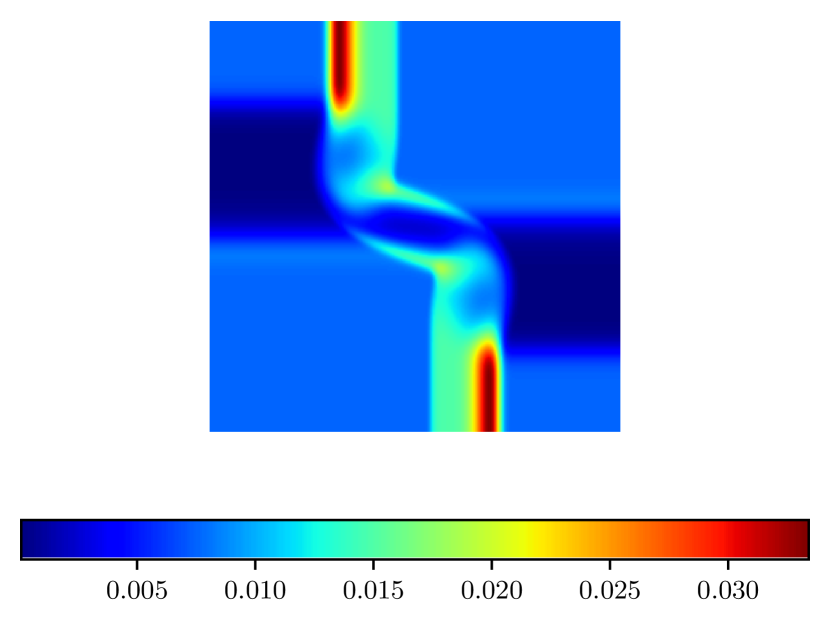
(a) Explicit, $\mathrm{CFL}=$0.9$$

(b) Jacobi method, $\mathrm{CFL}=$0.9$$

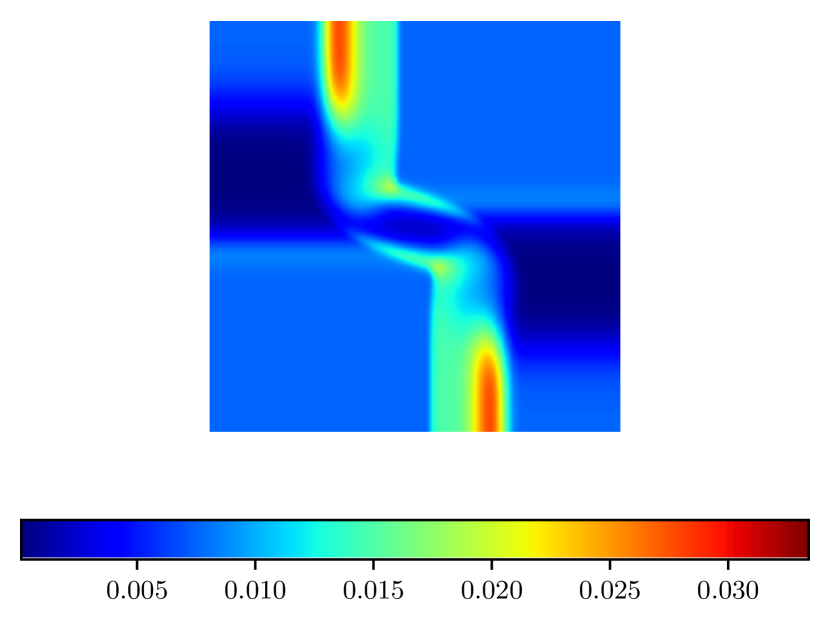
(c) Jacobi method, $\mathrm{CFL}=$2.7$$

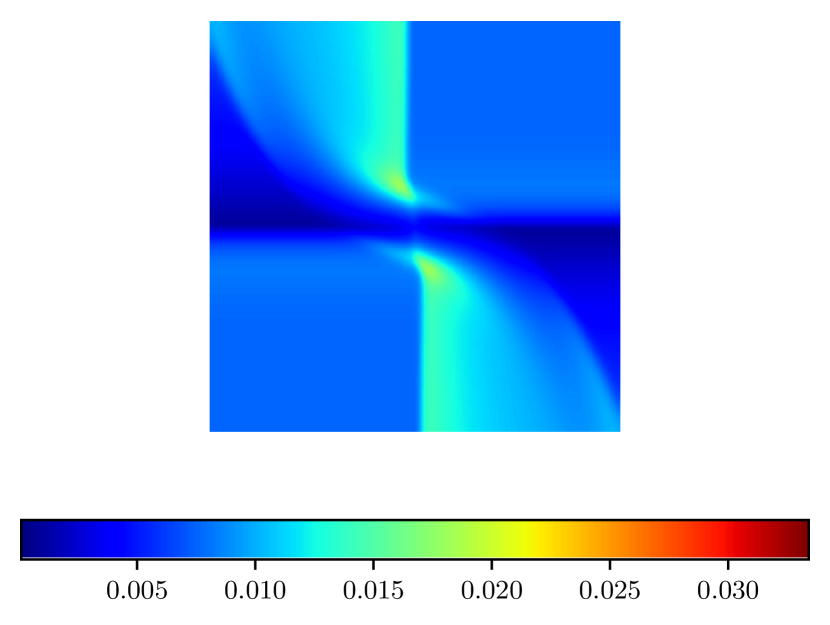
(d) Jacobi method, $\mathrm{CFL}=$150$$

Figure 11: Snapshots of radiative energy at final time $t_{f}=${10}^{-11}\text{\,}\mathrm{s}$$ with the explicit solver and the Jacobi method with different time steps.

Figure 11 shows snapshots of radiative energy at the final time ${10}^{-11}\text{\,}\mathrm{s}$ when Neumann boundary conditions are used. Different solutions are obtained with the explicit solver (fig. 11(a)) and Jacobi method with different time steps (figs. 11(b), 11(c) and 11(d)). The residual for the Jacobi method is set to $1\text{\times}{10}^{-6}$. As discussed in [31], the reduced flux stays close to $1$ during the simulation and the method is stable even for very stiff problems, with any time step. Because we use a scheme of order $1$, the solution is diffused, but the method preserves the admissible states with the reduced flux close to $1$. When small time steps are used with the Jacobi method (figs. 11(b) and 11(c)), we recover the explicit solution. When larger time steps are used (fig. 11(d)), the solution is more diffused. Because the flow is in the free-streaming regime and with sharp discontinuities, the propagation of the photons should be followed to capture with precision the solution of this problem. This can only be done by reducing the time step, close to the explicit time step. We do not expect an implicit method to be efficient in the test, but it shows that our scheme is extremely stable and robust, even at very large time steps. This feature is essential to carry out large and complex radiation hydrodynamics simulations, where the physics of interest will mostly be on hydrodynamical time scales.

6 Discussion and conclusion

We have first presented a Jacobi method to solve the nonlinear system arising from the discretization of the M₁ model without source terms with a time-implicit HLL solver. The admissible states are preserved, even with large CFL numbers. This method is iterative, the convergence rate decreases when the resolution increases. To tackle this issue, we use a nonlinear geometric multigrid algorithm. The Jacobi method first described is used as smoother and coarse grid solver. However, this algorithm relies on the residual equation, which does not preserve the admissible states. Instead of solving this equation, we introduce a pseudo-time, and we look for a steady state in pseudo-time. Numerical experiments have shown the good performances obtained with this algorithm. However, it should be used carefully in physical problems that require following the propagation of photons.

6.1 Source terms

In order to study physical problems, the integration of source terms is indispensable. It needs to be done carefully, regarding the asymptotic preserving property discussed in [9, 13] for example. The scheme should capture an asymptotic behavior in the diffusive limit. We did not address this issue here. For example, schemes presented in [22, 23, 14] are explicit, they preserve the admissible states, and they are asymptotic preserving. The HLL solver used here could be replaced by another scheme. This will change the nonlinear operator $\mathcal{A}$. It requires choosing carefully which terms are taken at iteration $k$ and $k+1$ in algorithm 1. The geometric multigrid algorithm presented in section 4 does not rely on the form of the nonlinear operator, as long as the iterations of the Jacobi method preserve the admissible states. Therefore, the geometric multigrid method can be used to study physical problems with opacity as soon as the Jacobi algorithm is extended to an asymptotic preserving scheme.

Similarly, the method could be extended to a non-gray model. We have defined the radiative energy (resp. radiative flux and radiative pressure) as the mean over the frequency and the direction of propagation of the photons of the specific intensity $I$ (resp. $I\mathbf{{\Omega}}$ and $I\mathbf{{\Omega}}\otimes\mathbf{{\Omega}}$). Therefore, our model does not take into account the frequency of the photons. One can use a multigroup model. The continuous frequency is discretized into several groups, and the variables are integrated over the frequency in each group. As previously, the Jacobi method could be adapted to this model. The main difficulty is to choose which terms are taken at iteration $k$ and $k+1$ in algorithm 1.

6.2 High-order scheme

In the numerical examples presented in section 5, the solution is more diffused than expected because a scheme of order $1$ is used. The numerical solution can be improved by increasing the order of the scheme. One method, among others, is spectral volume method (see e.g., [32]). Several degrees of freedom are added in the cell to reconstruct a polynomial. As with the finite volume method, the solution is discontinuous at the interfaces of the cells to capture shocks. This method is different from the Discontinuous Galerking method because it is based on the integral formulation of the equation instead of the weak formulation. The Runge-Kutta method can be used to achieve high-order in time.

Because the spectral volume method is close to the finite volume method, the Jacobi algorithm can be adapted to this scheme. As mentioned in [20], the pseudo-time introduced in section 4.3 is independent of the physical time. The discretization of eq. 29 is not required to be accurate, and an integration of order $1$ could be used.

In addition, a $p$-multigrid method can be used. A hierarchy is build and each level corresponds to a different approximation order.

However, we think that a high-order version of the algorithm is a significant amount of work, especially the inclusion of the reconstrution step in the non-linear jacobi and GMG method. This is part of our perspective for the future.

6.3 Performances

Although the performance results shown in section 5 are promising, some choices were made and others were not explored. For example, only a V-cycle is used, but there exist other possibilities: W-cycle, F-cycle,…The restriction and prolongation operators can also have an impact on the performances.

Another well-known method to reduce the number of iterations performed by the Jacobi method is to replace it with a Gauss-Seidel algorithm. Even though the tests presented in section 5 are obtained with a sequential code, we aim at using a parallel implementation to study physical situations. In the linear case, the Jacobi method is known to be easier to parallelize than the Gauss-Seidel method.

6.4 Parallel computing

The operator $\mathcal{A}$ considered here is nonlinear, due to the nonlinearity of the model. However, if this operator were linear, algorithm 1 would be the classical Jacobi method for a matrix-free problem. The pros and cons are the same as any multigrid method. For realistic computations, parallel computing is mandatory. The Jacobi method itself is quite easy to parallelize, as in the linear case. Because our approach can be seen as a matrix-free method, it can be parallelized using techniques developed for other equations. See for example [33] about the resolution of the Poisson equation using a parallel matrix-free multigrid method. Matrix-free algorithms are very suited for massively parallel computing because of their low memory footprint.

Appendix A Overall algorithm

Appendix A presents the whole algorithm to compute $\mathbf{{v}}^{n+1}$ with $\mathbf{{v}}^{n}$ known.

   4 Overall algorithm

 

1:Choose a maximum number of levels $L_{\max}$

2:$\kappa=0$

3:$\mathbf{{b}}^{h}=\mathbf{{v}}^{n}$

4:$\mathbf{{v}}^{h}_{(0)}=\mathbf{{v}}^{n}$. From now on, the exponent is the mesh size, it is no longer the time

5:while $\left\lvert\left\lvert\mathbf{{r}}_{(\kappa)}\right\lvert\right\lvert>\varepsilon$ do

6:     for $l=0,\cdots,L_{\max}-1$ do

7:         if $l=0$ then

8:              Pre-smoother: solve $\mathcal{A}^{h}\left(\mathbf{{u}}^{h}_{(\kappa)}\right)=\mathbf{{b}}^{h}$ with $\nu_{0}$ iterations of the nonlinear Jacobi method (algorithm 1), with initial guess $\mathbf{{v}}^{h}_{(\kappa)}$

9:              Compute residual: $\mathbf{{\overline{r}}}^{h}_{(\kappa)}=\mathbf{{b}}^{h}-\mathcal{A}^{h}\left(\mathbf{{u}}^{h}_{(\kappa)}\right)$

10:         else

11:              Pre-smoother: compute the steady state in pseudo-time of $\frac{\mathrm{d}\mathbf{{u}}^{2^{l}h}_{(\kappa)}}{\mathrm{d}\tau}+\mathcal{A}^{2^{l}h}\left(\mathbf{{u}}^{2^{l}h}_{(\kappa)}\right)=\mathcal{A}^{2^{l}h}\left(\mathbf{{v}}^{2^{l}h}_{(\kappa)}\right)+\mathbf{{r}}^{2^{l}h}_{(\kappa)}$ using algorithm 3, with $\nu_{l}$ iterations of the nonlinear Jacobi method , with initial guess $\mathbf{{v}}^{2^{l}h}_{(\kappa)}$

12:              Compute residual: $\mathbf{{\overline{r}}}^{2^{l}h}_{(\kappa)}=\mathcal{A}^{2^{l}h}\left(\mathbf{{v}}^{2^{l}h}_{(\kappa)}\right)+\mathbf{{r}}^{2^{l}h}_{(\kappa)}-\mathcal{A}^{2^{l}h}\left(\mathbf{{u}}^{2^{l}h}_{(\kappa)}\right)$

13:         end if

14:         Restriction: $\mathbf{{v}}^{2^{l+1}h}_{(\kappa)}=\mathcal{R}_{2^{l}h}^{2^{l+1}h}\left(\mathbf{{v}}^{2^{l}h}_{(\kappa)}\right)$ and $\mathbf{{r}}^{2^{l+1}h}_{(\kappa)}=\mathcal{R}_{2^{l}h}^{2^{l+1}h}\left(\mathbf{{\overline{r}}}^{2^{l}h}_{(\kappa)}\right)$

15:     end for

16:     Solver at the coarsest level: compute the steady state in pseudo-time of $\frac{\mathrm{d}\mathbf{{u}}^{2^{L_{\max}}h}_{(\kappa)}}{\mathrm{d}\tau}+\mathcal{A}^{2^{L_{\max}}h}\left(\mathbf{{u}}^{2^{L_{\max}}h}_{(\kappa)}\right)=\mathcal{A}^{2^{L_{\max}}h}\left(\mathbf{{v}}^{2^{L_{\max}}h}_{(\kappa)}\right)+\mathbf{{r}}^{2^{L_{\max}}h}_{(\kappa)}$ using algorithm 3, with $\nu_{L_{\max}}$ iterations of the nonlinear Jacobi method , with initial guess $\mathbf{{v}}^{2^{L_{\max}}h}_{(\kappa)}$

17:     for $l=L_{\max}-2,\cdots,0$ by step $-1$ do

18:         Prolongation: $\mathbf{{\overline{v}}}^{2^{l}h}_{(\kappa)}=\mathbf{{v}}^{2^{l}h}_{(\kappa)}+\mathcal{P}_{2^{l+1}h}^{2^{l}h}\left(\mathbf{{u}}^{2^{l+1}h}_{(\kappa)}-\mathbf{{v}}^{2^{l+1}h}_{(\kappa)}\right)$

19:         for each cell $l^{i}$ in the grid at level $l$ do

20:              if $\left(\mathbf{{\overline{v}}}^{2^{l}h}_{(\kappa)}\right)_{l^{i}}$ is not admissible then

21:                  use eq. 34 to update $\left(\mathbf{{\overline{v}}}^{2^{l}h}_{(\kappa)}\right)_{l^{i}}$

22:              end if

23:         end for

24:         if $l=0$ then

25:              Post-smoother: solve $\mathcal{A}^{h}\left(\mathbf{{u}}^{h}_{(\kappa)}\right)=\mathbf{{b}}^{h}$ with $\nu_{0}$ iterations of the nonlinear Jacobi method (algorithm 1), with initial guess $\mathbf{{\overline{v}}}^{h}_{(\kappa)}$

26:         else

27:              Post-smoother: compute the steady state in pseudo-time of $\frac{\mathrm{d}\mathbf{{u}}^{2^{l}h}_{(\kappa)}}{\mathrm{d}\tau}+\mathcal{A}^{2^{l}h}\left(\mathbf{{u}}^{2^{l}h}_{(\kappa)}\right)=\mathcal{A}^{2^{l}h}\left(\mathbf{{v}}^{2^{l}h}_{(\kappa)}\right)+\mathbf{{r}}^{2^{l}h}_{(\kappa)}$ using algorithm 3, with $\nu_{l}$ iterations of the nonlinear Jacobi method , with initial guess $\mathbf{{\overline{v}}}^{2^{l}h}_{(\kappa)}$

28:         end if

29:     end for

30:     $\mathbf{{v}}^{h}_{(\kappa)}=\mathbf{{u}}^{h}_{(\kappa)}$

31:     $\mathbf{{r}}_{(\kappa)}=\mathbf{{v}}^{n}-\mathcal{A}^{h}\left(\mathbf{{v}}^{h}_{(\kappa)}\right)$

32:     if $\frac{\left\lvert\left\lvert\left\lvert\mathbf{{r}}_{(\kappa)}\right\lvert\right\lvert-\left\lvert\left\lvert\mathbf{{r}}_{(\kappa-1)}\right\lvert\right\lvert\right\lvert}{\left\lvert\left\lvert\mathbf{{r}}_{(0)}\right\lvert\right\lvert}>\varepsilon_{i}$ then

33:         $\Delta\tau^{\text{im}}\leftarrow 1.1\Delta\tau^{\text{im}}$

34:     end if

35:     if $\frac{\left\lvert\left\lvert\left\lvert\mathbf{{r}}_{(\kappa)}\right\lvert\right\lvert-\left\lvert\left\lvert\mathbf{{r}}_{(\kappa-1)}\right\lvert\right\lvert\right\lvert}{\left\lvert\left\lvert\mathbf{{r}}_{(0)}\right\lvert\right\lvert}<\varepsilon_{d}$ then

36:         $\Delta\tau^{\text{im}}\leftarrow\Delta\tau^{\text{im}}/2$

37:     end if

38:     $\kappa\leftarrow\kappa+1$

39:end while

40:$\mathbf{{v}}^{n+1}=\mathbf{{v}}^{h}_{(\kappa)}$

References

- [1] A. Nascimento, Produire la santé, produire la sécurité : développer une culture collective de sécurité en radiothérapie, Ph.D. thesis (2009).
- [2] D. Christodoulou, The euler equations of compressible fluid flow, Bulletin of The American Mathematical Society (2007).
- [3] S. Chandrasekhar, Radiative Transfer, Dover Publications, 1960.
- [4] D. Mihalas, B. W. Mihalas, Foundations of radiation hydrodynamics, 1984.
- [5] R. B. Lowrie, H. M. Group, J. E. Morel, T. M. Group, J. A. Hittinger, M. . Department of Aerospace Engineering, Ann Arbor, The coupling of radiation and hydrodynamics, The Astrophysical Journal (1999).
- [6] J. H. Wise, T. Abel, Enzo+moray: radiation hydrodynamics adaptive mesh refinement simulations with adaptive ray tracing, Monthly notices of the Royal Astronomical Society (2011).
- [7] N. Roth, D. Kasen, Monte carlo radiation hydrodynamics with implicit methods, The Astrophysical Journal Supplement Series (2015).
- [8] C. D. Levermore, G. C. Pomraning, A flux-limited diffusion theory, The Astrophysical Journal (1981).
- [9] M. González, E. Audit, P. Huynh, Heracles: a three-dimensional radiation hydrodynamics code, Astronomy and Astrophysics (2007).
- [10] C. Levermore, Relating eddington factors to flux limiters, Journal of Quantitative Spectroscopy and Radiative Transfer (1984).
- [11] B. Dubroca, J.-L. Feugeas, Etude théorique et numérique d’une hiérarchie de modèles aux moments pour le transfert radiatif, Comptes Rendus de l’Académie des Sciences - Series I - Mathematics (1999).
- [12] D. Bertsekas, Nonlinear programming, Athena Scientific, 1995.
- [13] H. Bloch, P. Tremblin, M. González, T. Padioleau, E. Audit, A high-performance and portable asymptotic preserving radiation hydrodynamics code with the m1 model, Astronomy and Astrophysics (2021).
- [14] C. Berthon, R. Turpault, Asymptotic preserving hll schemes, Numerical Methods for Partial Differential Equations (2011).
- [15] C. Buet, B. Despres, Asymptotic preserving and positive schemes for radiation hydrodynamics, Journal of Computational Physics (2006).
- [16] T. Pichard, Mathematical modelling for dose depositon in photontherapy, Ph.D. thesis (2016).
- [17] T. Pichard, S. Brull, B. Dubroca, A numerical approach for a system of transport equations in the field of radiotherapy.
- [18] W. Briggs, V. Henson, S. McCormick, A multigrid tutorial, 2nd Edition, 2000.
- [19] A. Brandt, O. Livne, Multigrid techniques, 2011.
- [20] K. Kifonidis, E. Müller, On multigrid solution of the implicit equations of hydrodynamics - experiments for the compressible euler equations in general coordinates, Astronomy and Astrophysics (2012).
- [21] H. Bloch, Development and implementation of numerical schemes for radiation hydrodynamics, Ph.D. thesis (2021).
- [22] S. Jin, C. Levermore, Numerical schemes for hyperbolic conservation laws with stiff relaxation terms, Journal of Computational Physics (1996).
- [23] C. Buet, B. Despres, A gas dynamics scheme for a two moments model of radiative transfer (2008).
- [24] A. Harten, P. D. Lax, B. v. Leer, On upstream differencing and godunov-type schemes for hyperbolic conservation laws, SIAM Review (1983).
- [25] V. Rusanov, The calculation of the interaction of non-stationary shock waves and obstacles, USSR Computational Mathematics and Mathematical Physics (1962).
- [26] Y. Saad, Iterative methods for sparse linear systems, 2003.
- [27] S. Richling, E. Meinköhn, N. Kryzhevoi, G. Kanschat, Radiative transfer with finite elements - i. basic method and tests, Astronomy and Astrophysics (2001).
- [28] M. Gander, S. Loisel, D. Szyld, An optimal block iterative method and preconditioner for banded matrices with applications to pdes on irregular domains, SIAM Journal on Matrix Analysis and Applications (04 2010).
- [29] G. Strang, Multigrid methods (2006).
- [30] H. Van der Vorst, Bi-cgstab: A fast and smoothly converging variant of bi-cg for the solution of nonsymmetric linear systems, SIAM Journal on Scientific and Statistical Computing (1992).
- [31] F. Blachère, R. Turpault, An admissibility and asymptotic-preserving scheme for systems of conservation laws with source term on 2d unstructured meshes, Journal of Computational Physics (2016).
- [32] T. Padioleau, Development of ”all-régime” AMR simulation methods for fluid dynamics, application in astrophysics and two-phase flows, Ph.D. thesis (2020).
- [33] N. Kohl, U. Rüde, Textbook efficiency: massively parallel matrix-free multigrid for the stokes system, SIAM Journal on Scientific Computing (2022).