Let us Build Bridges: Understanding and Extending Diffusion Generative Models

Abstract

Diffusion-based generative models have achieved promising results recently, but raise an array of open questions in terms of conceptual understanding, theoretical analysis, algorithm improvement and extensions to discrete, structured, non-Euclidean domains. This work tries to re-exam the overall framework, in order to gain better theoretical understandings and develop algorithmic extensions for data from arbitrary domains. By viewing diffusion models as latent variable models with unobserved diffusion trajectories and applying maximum likelihood estimation (MLE) with latent trajectories imputed from an auxiliary distribution, we show that both the model construction and the imputation of latent trajectories amount to constructing diffusion bridge processes that achieve deterministic values and constraints at end point, for which we provide a systematic study and a suit of tools. Leveraging our framework, we present 1) a first theoretical error analysis for learning diffusion generation models, and 2) a simple and unified approach to learning on data from different discrete and constrained domains. Experiments show that our methods perform superbly on generating images, semantic segments and 3D point clouds.

1 Introduction

Diffusion-based deep generative models, notably score matching with Langevin dynamics (SMLD) (Song and Ermon, 2019, 2020), denoising diffusion probabilistic models (DDPM) (Ho et al., 2020), and their variants (e.g., Song et al., 2020b, a; Kong and Ping, 2021; Song et al., 2021; Nichol and Dhariwal, 2021), have shown to achieve new state of the art results for image synthesis (Dhariwal and Nichol, 2021; Ramesh et al., 2022; Ho et al., 2022; Liu et al., 2021), audio synthesis (Chen et al., 2020; Kong et al., 2020), point cloud synthesis Luo and Hu (2021a, b); Zhou et al. (2021), and many other AI tasks. These methods train a deep neural network to drive as drift force a diffusion process to generate data, and are shown to outperform competitors, mainly GANs and VAEs, on stability and sample diversity (Xiao et al., 2021; Ho et al., 2020; Song et al., 2020b).

However, a range of open challenges arise on understanding, analyzing, and improving diffusion-based models. On the conceptual and theoretical perspective, existing methods have been derived from multiple angles, including denoising score matching (Vincent, 2011; Song and Ermon, 2019), time reversed diffusion (Song et al., 2020b), and variational bounds (Ho et al., 2020), but these approaches leave many design choices whose relations and effects have been unclear and difficult to analyze. On the practical side, standard approaches tend to be slow in both training and inference due to the need of a large number of diffusion steps, and are restricted to generating continuous data in $\mathbb{R}^{d}$ – special techniques such as dequantization (Uria et al., 2013; Ho et al., 2019) and multinomial diffusion (Hoogeboom et al., 2021; Austin et al., 2021) need to be developed case by case for different types of discrete data and the results still tend to be unsatisfying despite promising recent advances Hoogeboom et al. (2021); Austin et al. (2021).

In this work, we approach diffusion models with a simple and classical statistical learning framework. By viewing the diffusion models as a latent variable model consisting of unobserved trajectories whose end points output observed data, the learning is decomposed into two parts: 1) constructing imputation mechanisms to generate latent trajectories that would have generated a given data point $x$, and 2) specifying and training the diffusion generative model to generate data on the domain $\Omega$ of interest by maximizing likelihood using the imputed trajectories. Both components involve constructing diffusion bridge processes, called $x$-bridge and $\Omega$-bridge, whose end points guarantee to hit a deterministic value $x$ or domain $\Omega$ at the terminal time, respectively. The design of learning algorithms reduces to constructing two bridges, for both which we provide a systematic study and a full suit of techniques. Our framework allows us to decouple the various building blocks of the diffusion learning, enabling new theoretical analysis, algorithmic extensions to structured domains, and speedup in the regime of small sampling steps. Among others, we want to highlight two particular contributions:

1) We develop a first error analysis for learning diffusion models including both statistical errors and time-discretization errors. In regime of classical asymptotic statistics (Van der Vaart, 2000), we show that the KL divergence between the true and learned distributions from a variant of our method has an asymptotic rate of ${O}{\left((\log(1/\epsilon)+1)/n+\epsilon\right)}$, where $n$ is the number of i.i.d. data points and $\epsilon$ the step size in Euler discretization of the SDEs.

2) Our framework is instantiated to provide a simple and universal approach to learning on data from an arbitrary domain $\Omega$ that can be embedded in $\mathbb{R}^{d}$ and on which the expectation of truncated standard Gaussian distribution can be evaluated. This includes product spaces of any type, bounded/unbounded, continuous/discrete, categorical/ordinal data, and their mix. The efficiency of the method is testified on a suit of examples, including generating images, segmentation maps, and grid-valued point clouds.

2 Learning Latent Diffusion Models

Diffusion Generative Models

Figure 1: $\Omega$-Bridges for discrete $\Omega=\{1,2,3,4\}$.

Let $\{x^{(i)}\}_{i=1}^{n}$ be an i.i.d. sample from an unknown distribution ${\Pi^{*}}$ on a domain $\Omega\subseteq\mathbb{R}^{d}$. We want to fit the data with a diffusion model $\mathbb{P}^{\theta}(\mathrm{d}Z)$, which specifies the distribution of a latent trajectory $Z=\{Z_{t}\colon t\in[0,{{T}}]\}$ that outputs an observation ($x=Z_{{T}}$) at the terminal time ${{T}}$. The evolution of $Z$ is governed by an Ito process:

$$\mathrm{d}Z_{t}=s^{\theta}_{t}(Z_{t})\mathrm{d}t+\sigma_{t}(Z_{t})\mathrm{d}W_{t},~{}~{}\forall t\in[0,{{T}}],~{}~{}~{}~{}~{}~{}~{}Z_{0}\sim{\mathbb{P}_{0}^{\theta}},$$ (1)

where $W_{t}$ is a Wiener process; $\sigma\colon[0,{{T}}]\times\mathbb{R}^{d}\to\mathbb{R}^{d\times d}$ is a fixed, positive definite diffusion coefficient; the drift term $s^{\theta}\in[0,{{T}}]\times\mathbb{R}^{d}\to\mathbb{R}^{d}$ depends on a trainable parameter $\theta$ and is often specified using a deep neural network. The initial distribution $\mathbb{P}_{0}^{\theta}$ is often a fixed elementary distribution (Gaussian or deterministic), but we keep it trainable in the general framework. Here, $\mathbb{P}^{\theta}$ is the path measure on continuous trajectories $Z$ following (1). We denote by $\mathbb{P}_{t}^{\theta}$ the marginal distribution of $Z_{t}$ at time $t$. We want to estimate $\theta$ such that the terminal distribution $Z_{{T}}\sim\mathbb{P}_{{T}}^{\theta}$ matches the data $X\sim{\Pi^{*}}$.

If $\Omega$ is a strict subset of $\mathbb{R}^{d}$, e.g., bounded or discrete, then we need to specify the model $\mathbb{P}^{\theta}$ in (1) such that $Z_{{T}}$ is guaranteed to arrive $\Omega$ at $t={{T}}$ (while the non-terminal states may not belong to $\Omega$).

☞ A process $Z$ in $\mathbb{R}^{d}$ with law $\mathbb{P}$ is called a bridge to a set $B\subset\mathbb{R}^{d}$, or $B$-bridge, if $\mathbb{P}(Z_{{T}}\in B)=1$.

Section 3.5 discusses how to specify $s^{\theta}$ such that $\mathbb{P}^{\theta}$ is an $\Omega$-bridge. We assume $\Omega=\mathbb{R}^{d}$ for now.

A Poor man’s EM

A canonical approach to learning latent variable models like $\mathbb{P}^{\theta}$ is (variational) expectation maximization (EM), which alternates between 1) estimating the posterior distribution $\mathbb{P}^{\theta,x}\coloneqq\mathbb{P}^{\theta}(Z|Z_{{T}}=x)$ of the latent trajectories $Z$ given the observation (E-step), and 2) estimating the model parameter $\theta$ with $Z$ imputed from $\mathbb{P}^{\theta,x}$ (M-step). Following DDPM (Ho et al., 2020), we consider a simpler approach consisting of only the M-step, estimating $\theta$ with $Z$ drawn from ${\mathbb{Q}}^{x}\coloneqq{\mathbb{Q}}(Z|Z_{{T}}=x)$ of a pre-specified simple baseline process ${\mathbb{Q}}$, rather than the more expensive $\mathbb{P}^{\theta,x}$. Here for each $x\in\Omega$, the conditioned process ${\mathbb{Q}}^{x}\coloneqq{\mathbb{Q}}(Z|Z_{{T}}=x)$ is the distribution of the trajectories from ${\mathbb{Q}}$ that are pinned at $x$ at time $t$. Therefore, ${\mathbb{Q}}^{x}$ is an $x$-bridge by definition.

Let ${\mathbb{Q}}^{\Pi^{*}}(\cdot)=\int{\mathbb{Q}}^{x}(\cdot){\Pi^{*}}(\mathrm{d}x)$ be the distribution of trajectories $Z$ generated in the following “backward” way: first drawing a data point $x\sim{\Pi^{*}}$, and then $Z\sim{\mathbb{Q}}^{x}$ conditioned on the end point $x$. This construction ensures that the terminal distribution of ${\mathbb{Q}}^{\Pi^{*}}$ equals ${\Pi^{*}}$, that is, ${\mathbb{Q}}^{\Pi^{*}}_{{T}}={\Pi^{*}}$. Then, the model $\mathbb{P}^{\theta}$ can be estimated by fitting data drawn from ${\mathbb{Q}}^{\Pi^{*}}$ using maximum likelihood estimator:

$$\min_{\theta}\left\{{\mathcal{L}}(\theta)\coloneqq\mathcal{KL}({\mathbb{Q}}^{\Pi^{*}}~{}||~{}\mathbb{P}^{\theta})\right\}.$$ (2)

The classical (variational) EM would alternatively update $\theta$ (M-step) and ${\mathbb{Q}}^{x}$ (E-step) to make ${\mathbb{Q}}^{x}\approx\mathbb{P}^{\theta,x}$. Why is it ok to simply drop the E-step? At the high level, it is the benefit from using universal approximators like deep neural networks: if the model space of $\mathbb{P}^{\theta}$ is sufficiently rich, by minimizing the KL divergence in (2), $\mathbb{P}^{\theta}$ can approximate the given ${\mathbb{Q}}^{\Pi^{*}}$ well enough (in a way that is made precise in sequel) such that their terminal distributions are close: $\mathbb{P}^{\theta}_{{T}}\approx{\mathbb{Q}}^{\Pi^{*}}_{{T}}={\Pi^{*}}$.

☞ Learning latent variable models require no E-step if the model space is sufficiently rich.

We should see that in this case the latent variables $Z$ in the learned model $\mathbb{P}^{\theta}$ is dictated by the choice of the imputation distribution ${\mathbb{Q}}$ since we have $\mathbb{P}^{\theta,x}={\mathbb{Q}}^{x}$ when the KL divergence in (2) is fully minimized to zero; EM also achieves $\mathbb{P}^{\theta,x}={\mathbb{Q}}^{x}$ but has the imputation distribution ${\mathbb{Q}}^{x}$ determined by the model $\mathbb{P}^{\theta}$, not the other way.

Loss Function

Let us assume that ${\mathbb{Q}}^{x}$ yields a general non-Markov diffusion process of form

$$\mathrm{d}Z_{t}=\eta^{x}(Z_{[0,t]},t)\mathrm{d}t+\sigma(Z_{t},t)\mathrm{d}W_{t},~{}~{}~{}~{}~{}Z_{0}\sim\mu^{x},$$ (3)

where the drift $\eta^{x}$ and initial distribution $\mu^{x}$ depend on the end point $x$ and the diffusion coefficient $\sigma$ is the same as that of $\mathbb{P}^{\theta}$. Here $\eta^{x}$ can depend on the whole trajectory upto time $t$ and hence ${\mathbb{Q}}^{x}$ can be non-Markov. ${\mathbb{Q}}^{x}$ is Markov if $\eta^{x}(Z_{[0,t]},t)=\eta^{x}(Z_{t},t).$ See Section 3 for instances of $\eta^{x},\mu^{x}$.

Using Girsanov theorem (e.g., Oksendal, 2013), with $\mathbb{P}^{\theta}$ in (1) and ${\mathbb{Q}}^{x}$ in (3), the KL divergence in (2) can be reframed into a form of the score matching loss from Song et al. (2020b, 2021):

$${\mathcal{L}}(\theta)=\mathbb{E}_{\begin{subarray}{c}x\sim{\Pi^{*}}\\ Z\sim{\mathbb{Q}}^{x}\end{subarray}}\!\!\!\left[\underbrace{-\log p_{0}^{\theta}(Z_{0})}_{\text{MLE of initial dist.}}+\frac{1}{2}\int_{0}^{{T}}\!\!\!\underbrace{\left\lVert\sigma^{-1}(Z_{t},t)(s^{\theta}(Z_{t},t)-\eta^{x}(Z_{[0,t]},t))\right\rVert^{2}}_{\text{score matching}}\!\mathrm{d}t\right]+const,$$ (4)

where $p_{0}^{\theta}$ is the probability density function (PDF) of the initial distribution $\mathbb{P}^{\theta}_{0}$. Therefore, ${\mathcal{L}}(\theta)$ is a sum of the negative log-likelihood of the initial distribution that encourages $\mathbb{P}_{0}^{\theta}\approx{\mathbb{Q}}^{\Pi^{*}}_{0}$, and a least squares loss between $s^{\theta}$ and $\eta^{x}$. See practical implementation in Section 4 and Algorithm 1.

Markovization

As $\mathbb{P}^{\theta}$ is Markov by the model assumption, it can not perfectly fit ${\mathbb{Q}}^{\Pi^{*}}$ which is non-Markov in general. This is a substantial problem because ${\mathbb{Q}}^{\Pi^{*}}$ can be non-Markov even if ${\mathbb{Q}}^{x}$ is Markov for all $x\in\Omega$ (see Section 3.4). In fact, using Doob’s $h$-transform method (Doob and Doob, 1984), ${\mathbb{Q}}^{\Pi^{*}}$ can be shown to be the law of a diffusion process

$$\mathrm{d}Z_{t}=\eta^{\Pi^{*}}(Z_{[0,t]},t)\mathrm{d}t+\sigma(Z_{t},t)\mathrm{d}W_{t}, \eta^{\Pi^{*}}(z_{[0,t]},t)=\mathbb{E}_{Z\sim{\mathbb{Q}}^{\Pi^{*}}}\left[\eta^{Z_{{T}}}(z_{[0,t]},t)~{}|~{}Z_{[0,t]}=z_{[0,t]}\right],$$

where $\eta^{\Pi^{*}}$ is the expectation of $\eta^{x}$ when $x=Z_{{T}}$ is drawn from ${\mathbb{Q}}$ conditioned on $Z_{[0,t]}$.

We resolve this by observing that it is not necessary to match the whole path measure ($\mathbb{P}^{\theta}\approx{\mathbb{Q}}^{\Pi^{*}}$) to match the terminal ($\mathbb{P}_{{T}}^{\theta}\approx{\mathbb{Q}}_{{T}}^{\Pi^{*}}={\Pi^{*}}$). It is enough for $\mathbb{P}^{\theta}$ to be the best Markov approximation (a.k.a. Markovization) of ${\mathbb{Q}}^{\Pi^{*}}$, which matches all (hence terminal) fixed-time marginals with ${\mathbb{Q}}^{\Pi^{*}}$:

$$\mathrm{Proj}({\mathbb{Q}}^{\Pi^{*}},\mathcal{M})\coloneqq\operatorname*{arg\,min}_{\mathbb{P}\in\mathcal{M}}\mathcal{KL}({\mathbb{Q}}^{\Pi^{*}}~{}||~{}\mathbb{P}), \text{$\mathcal{M}$ = the set of all Markov processes on $[0,{{T}}]$}.$$

Proposition 2.1.

The global optimum of ${\mathcal{L}}(\theta)$ in (2) and (4) is achieved by $\theta^{*}$ if

$$s^{\theta^{*}}(z,t)=\mathbb{E}_{Z\sim{\mathbb{Q}}^{\Pi^{*}}}\left[\eta^{Z_{{T}}}(Z_{[0,t]},t)~{}|~{}Z_{t}=z\right], \mu^{\theta^{*}}(\mathrm{d}z_{0})={\mathbb{Q}}^{\Pi^{*}}_{0}=\mathbb{E}_{x\sim{\Pi^{*}}}\left[{{\mathbb{Q}}}_{0}^{x}(\mathrm{d}z_{0})\right].$$ (5)

In this case, $\mathbb{P}^{\theta^{*}}=\mathrm{Proj}({\mathbb{Q}}^{\Pi^{*}},\mathcal{M})$ is the Markovization of ${\mathbb{Q}}^{\Pi^{*}}$, with which it matches all time-marginals: $\mathbb{P}^{\theta^{*}}_{t}={\mathbb{Q}}^{\Pi^{*}}_{t}$ for all time $t\in[0,T]$. In addition,

$$\mathcal{KL}({\Pi^{*}}~{}||~{}\mathbb{P}^{\theta}_{{T}})\leq\mathcal{KL}(\mathbb{P}^{\theta^{*}}~{}||~{}\mathbb{P}^{\theta})=\mathcal{KL}({\mathbb{Q}}^{\Pi^{*}}~{}||~{}\mathbb{P}^{\theta})-\mathcal{KL}({\mathbb{Q}}^{\Pi^{*}}~{}||~{}\mathbb{P}^{\theta^{*}})={\mathcal{L}}(\theta)-{\mathcal{L}}(\theta^{*}).$$ (6)

Note that $s^{\theta^{*}}$ is a conditional expectation of $\eta^{\Pi^{*}}$: $s^{\theta^{*}}(z,t)=\mathbb{E}_{Z\sim{\mathbb{Q}}^{\Pi^{*}}}[\eta^{{\Pi^{*}}}(Z_{[0,t]},t)~{}|~{}Z_{t}=z].$ Theorem 1 of Peluchetti (2021) gives a related result that the marginals of mixtures of Markov diffusion processes can be matched by another Markov diffusion process, but does not discuss the issue of Markovization nor connect to KL divergence. Theorem 1 of Song et al. (2021) is the special case of (6) when ${\mathbb{Q}}^{\Pi^{*}}$ is Markov.

Algorithm 1 Learning diffusion generative models on domain $\Omega\subseteq\mathbb{R}^{d}$

  Input: Given a dataset $\{x^{(i)}\}$ drawn from distribution ${\Pi^{*}}$ on domain $\Omega\subseteq\mathbb{R}^{d}$, learn a diffusion model $\mathbb{P}^{\theta}$.

  1) Take a baseline process ${\mathbb{Q}}$, find an $x$-bridge ${\mathbb{Q}}^{x}$ and set the model $\mathbb{P}^{\theta}$ to be $\Omega$-bridges as in (12).

  2) Estimate $\theta$ by minimizing $\hat{\mathcal{L}}(\theta)$ in (13) with stochastic gradient descent.

  3) Draw approximate sample from $\mathbb{P}^{\theta}$ following (14).

  Remark If we initialize ${\mathbb{Q}}^{x}$ from a common distribution $\mu^{x}=\mu$, we can set $\mathbb{P}_{0}^{\theta}=\mu$ and drop the initial log-likelihood term $\log p_{0}^{\theta}$ in (13).

3 Let us Build Bridges

We discuss how to build bridges, both ${\mathbb{Q}}^{x}$ as $x$-bridges and $\mathbb{P}^{\theta}$ as $\Omega$-bridges for constrained domains. We first derive ${\mathbb{Q}}^{x}$ as the conditioned process ${\mathbb{Q}}(\cdot|Z_{{T}}=x)$ by using time reversal and $h$-transform (Section 3.1-3.2), and then construct new bridges using mixtures of existing bridges which allows us to decouple the choice of initialization and dynamics in bridges (Section 3.3) and clarify the Markov property of the resulting ${\mathbb{Q}}^{\Pi^{*}}$ (Section 3.4). In Section 3.5, we provide a general approach for constructing $\mathbb{P}^{\theta}$ as $\Omega$-bridges for constrained domains.

3.1 Bridge Construction: Time Reversal

SMLD and DDPM can be viewed as specifying ${\mathbb{Q}}$ via its time-reversed process that starts at time ${{T}}$ and proceed backwards to $t=0$. The conditioning on $Z_{{T}}=x$ can be achieved by simply initializing the reversed process from $x$. Specifically, ${\mathbb{Q}}^{x}$ is defined as the law of $Z_{t}^{x}$ whose reversed process $\tilde{Z}_{t}^{x}\coloneqq Z_{{{T}}-t}^{x}$ follows a Markov diffusion process that starts at $\tilde{Z}_{0}^{x}=x$:

$$\mathrm{d}\tilde{Z}_{t}^{x}=\tilde{\eta}(\tilde{Z}_{t}^{x},{{T}}-t)\mathrm{d}t+\sigma(\tilde{Z}_{t}^{x},{{T}}-t)\mathrm{d}\tilde{W}_{t},~{}~{}~{}~{}~{}~{}~{}~{}~{}\tilde{Z}_{0}^{x}=x,$$ (7)

where $\tilde{W}$ is a standard Brownian motion. Using the time reversion formula (e.g., Anderson, 1982), $Z_{t}^{x}$ follows

$$\mathrm{d}Z_{t}^{x}=\left(-\tilde{\eta}(Z_{t}^{x},t)+\frac{\nabla_{z}(\sigma^{2}(Z^{x}_{t},t)q^{x}_{t}(Z^{x}_{t}))}{q^{x}_{t}(Z^{x}_{t})}\right)\mathrm{d}t+\sigma(Z_{t}^{x},t)\mathrm{d}W_{t},~{}~{}~{}~{}~{}~{}~{}~{}~{}Z_{0}^{x}\sim{\mathbb{Q}}^{x}_{0},$$ (8)

where $\sigma^{2}=\sigma\sigma^{\top}$ denotes matrix square, and ${\mathbb{Q}}_{t}^{x}$ and $q_{t}^{x}$ are the distribution and density function of $Z^{x}_{t}=\tilde{Z}^{x}_{{{T}}-t}$ following (7), which formula needs to be derived.

As summarized in Song et al. (2020b), most existing works specify (7) as an Ornstein–Uhlenbeck (O-U) process of form $\mathrm{d}\tilde{Z}_{t}=-\alpha_{{{T}}-t}\tilde{Z}_{t}\mathrm{d}t+\varsigma_{{{T}}-t}\mathrm{d}\tilde{W}_{t}$. In particular, SMLD (Song and Ermon, 2019, 2020) uses $\alpha_{t}=0$ (Variance Exploding (VE) SDE) and DDPM uses $\alpha_{t}=\varsigma_{t}^{2}/2$ (Variance Preserving (VP) SDE).

Example 3.1.

SMLD (Song and Ermon, 2019, 2020) uses $\mathrm{d}\tilde{Z}^{x}_{t}=\varsigma_{{{T}}-t}\mathrm{d}\tilde{W}_{t}$. Let $\beta_{t}=\int_{0}^{t}\varsigma_{s}^{2}\mathrm{d}s$. Then $Z^{x}_{t}=\tilde{Z}^{x}_{{{T}}-t}$ follows

$$\mathrm{d}Z^{x}_{t}=\eta_{\mathrm{bb},\varsigma}^{x}(Z^{x}_{t},t)\mathrm{d}t+\varsigma_{t}\mathrm{d}W_{t}, \eta_{\mathrm{bb},\varsigma}^{x}(Z^{x}_{t},t)=\varsigma_{t}^{2}\frac{x-Z^{x}_{t}}{\beta_{{T}}-\beta_{t}} Z^{x}_{0}\sim\mathcal{N}(x,\beta_{{T}})$$ with     and , (9)

which is a Brownian bridge (BB) process. A simple case is when $\varsigma_{t}=1$ and $\eta_{\mathrm{bb},1}^{x}(z,t)=\frac{x-z}{{{T}}-t}$.
Because the initial distribution ${\mathbb{Q}}^{x}_{0}=\mathcal{N}(x,\beta_{{T}})$ depends on data $x$, the initial distribution $\mathbb{P}_{0}^{\theta}$ of $\mathbb{P}^{\theta}$ should in principle be learned to fit the mixture $\int{\mathbb{Q}}^{x}_{0}{\Pi^{*}}(\mathrm{d}x)$. But as suggested in SMLD, we can set $\mathbb{P}_{0}^{\theta}=\mathcal{N}(0,\beta_{{T}})$ as an approximation when $\beta_{{T}}$ is very large compared to the variance of the data ${\Pi^{*}}$.

3.2 Bridge Construction: $h$-transform

The conditioned process can be derived directly without resorting to time reversal Peluchetti (2021). Assume ${\mathbb{Q}}$ follows $\mathrm{d}Z_{t}=b(Z_{t},t)\mathrm{d}t+\sigma(Z_{t},t)\mathrm{d}W_{t}$. Then by using Doob’s method of $h$-transforms (Oksendal, 2013), the conditioned process ${\mathbb{Q}}^{x}(\cdot)\coloneqq{\mathbb{Q}}(\cdot~{}|~{}Z_{{T}}=x)$, if it exists, can be shown to be the law of

$$\mathrm{d}Z^{x}_{t}=\left(b(Z^{x}_{t},t)+{\sigma^{2}(Z^{x}_{t},t)\nabla_{z}\log q_{{{T}}|t}(x~{}|~{}Z^{x}_{t})}\right)\mathrm{d}t+\sigma(Z_{t}^{x},t)\mathrm{d}W_{t},~{}~{}~{}~{}Z_{0}\sim{\mathbb{Q}}_{0|T}(\cdot~{}|~{}x),$$ (10)

where $q_{{{T}}|t}(x|z)$ is the density function of the transition probability ${\mathbb{Q}}_{{{T}}|t}(\mathrm{d}x|z)={\mathbb{Q}}(Z_{{T}}\in\mathrm{d}x|Z_{t}=z)$, assuming it exists. The additional drift term $\sigma^{2}\nabla\log q_{{{T}}|t}(x|z)$ plays the role of steering $Z_{t}$ towards the target $Z_{{T}}=x$. The initial distribution can be calculated by Bayes rule: ${\mathbb{Q}}_{0|T}(\mathrm{d}z|x)\propto{\mathbb{Q}}_{0}(\mathrm{d}z)q_{{{T}}|0}(x|z)$. We should note that the drift term in (10) is independent of the initialization ${\mathbb{Q}}_{0}$, which allows us to decouple in Section 3.3 the choices of initialization and drift in bridges.

Example 3.2.

If ${\mathbb{Q}}$ is the law of $\mathrm{d}Z_{t}=\varsigma_{t}\mathrm{d}W_{t}$, we have ${\mathbb{Q}}_{{{T}}|t}(\cdot|z)=\mathcal{N}(z,\beta_{{T}}-\beta_{t})$, where $\beta_{t}=\int_{0}^{t}\varsigma_{s}^{2}\mathrm{d}s$. Hence ${\mathbb{Q}}^{x}={\mathbb{Q}}(\cdot|Z_{{T}}=x)$ is the law of

$$\mathrm{d}Z_{t}^{x}=\eta_{\mathrm{bb},\varsigma}^{x}(Z^{x}_{t},t)\mathrm{d}t+\varsigma_{t}\mathrm{d}W_{t}, Z^{x}_{0}\sim{\mathbb{Q}}^{x}_{0}={\mathbb{Q}}_{0|T}(\cdot|x)$$ with     , (11)

where ${\mathbb{Q}}_{0}^{x}(\mathrm{d}z)\propto{\mathbb{Q}}_{0}(\mathrm{d}z)\phi(x~{}|~{}z,\beta_{{T}}-\beta_{t})$, and $\phi(\cdot|\mu,\sigma^{2})$ is the density function of $\mathcal{N}(\mu,\sigma^{2}).$

The ${\mathbb{Q}}^{x}$ in (11) shares the same drift $\eta^{x}_{\mathrm{bb},\varsigma}$ as that of SMLD in (9), but has a different initialization that depends on ${\mathbb{Q}}_{0}$. Two extreme choices of ${\mathbb{Q}}_{0}$ stand out:

1) The SMLD initialization can be viewed as the case when we initialize ${\mathbb{Q}}$ with an improper “uniform” prior ${\mathbb{Q}}_{0}=1$, corresponding ${\mathbb{Q}}_{0}=\mathcal{N}(0,v)$ with $v\to+\infty$. DDPM can be similarly interpreted as taking ${\mathbb{Q}}$ to be a forward time O-U process $\mathrm{d}Z_{t}=\alpha_{t}Z_{t}\mathrm{d}t+\varsigma_{t}\mathrm{d}W_{t}$ with an improper uniform initialization ${\mathbb{Q}}_{0}=1$ (see more discussion in Appendix).

2) Let $z_{0}$ be any point that can reach $Z_{{T}}=x$ under ${\mathbb{Q}}$ in that $x\in\mathrm{supp}({\mathbb{Q}}_{{{T}}|0}(\cdot|z))$. If we take ${\mathbb{Q}}_{0}=\delta_{z_{0}}$, the delta measure centered at $z_{0}$, the bridge ${\mathbb{Q}}^{x}$ has the same deterministic initialization ${\mathbb{Q}}^{x}_{0}=\delta_{z_{0}}$. Hence any deterministic initialization equipped with the drift in (10) yields a conditional bridge. This choice is particularly convenient because ${\mathbb{Q}}^{x}_{0}$ is independent of $x$, and hence $\mathbb{P}^{\theta}$ can be initialized at $\mathbb{P}_{0}^{\theta}=\delta_{z}$ without learning.

3.3 Bridge Construction: Mixtures

It is an immediate observation that mixtures of bridges are bridges: Let ${\mathbb{Q}}^{z,A}$ be a set of $A$-bridges indexed by a variable $z$, then ${\mathbb{Q}}^{A}\coloneqq\int{\mathbb{Q}}^{z,A}\mu(\mathrm{d}z)$ is an $x$-bridge for any distribution $\mu$ on $z$.

A special case is to take the mixture of the conditional bridges in (10) starting from different deterministic initialization, which shows that we can obtain a valid $x$-bridge by equipping the same drift in (10) with essentially any initialization. Hence, the choices of the drift force and initialization in ${\mathbb{Q}}^{x}$ can be completely decouple, which is not obvious from the time reversal framework, since there different dynamics (e.g., VP-SDE, VE-SDE) have to designed to obtain different ${\mathbb{Q}}_{0}^{x}$.

Proposition 3.3.

Let $\tilde{\mathbb{Q}}$ is a path measure and $\Omega_{x}$ is the set of $z$ for which $\tilde{\mathbb{Q}}^{z_{0},x}(\cdot)\coloneqq\tilde{\mathbb{Q}}(\cdot|Z_{{T}}=x,Z_{0}=z_{0})$ exists. Then ${\mathbb{Q}}^{x}\coloneqq\int\tilde{\mathbb{Q}}^{z_{0},x}\mu(\mathrm{d}z_{0}~{}|~{}x)$ is an $x$-bridge, for any distribution $\mu$ on $\Omega\times\Omega$.

3.4 Markov and Reciprocal Structures of ${\mathbb{Q}}^{\Pi^{*}}$

If ${\mathbb{Q}}^{x}$ is constructed as ${\mathbb{Q}}^{x}={\mathbb{Q}}(\cdot|Z_{{T}}=x)$, it is easy to see that ${\mathbb{Q}}^{\Pi^{*}}$ is Markov iff ${\mathbb{Q}}$ is Markov. If ${\mathbb{Q}}^{x}$ is constructed from mixtures of bridges as above, the resulting ${\mathbb{Q}}^{\Pi^{*}}$ is more complex. In fact, simply varying the initialization $\mu$ in Proposition (3.3) can change the Markov structure of ${\mathbb{Q}}^{\Pi^{*}}$.

Proposition 3.4.

Take ${\mathbb{Q}}^{x}$ to be the dynamics in (11) initialized from $Z_{0}\sim\mathcal{N}(0,v_{0})$. Assume $\varsigma_{t}>0$, $\forall t\in[0,{{T}}]$. Then ${\mathbb{Q}}^{\Pi^{*}}$ is Markov only when $v_{0}=0$, or $v_{0}=+\infty$.

The right characterization of ${\mathbb{Q}}^{\Pi^{*}}$ from Proposition (3.3) involves reciprocal processes (Léonard et al., 2014).

Definition 3.5.

A process $Z$ with law ${\mathbb{Q}}$ on $[0,T]$ is said to be reciporcal if it can be written into ${\mathbb{Q}}=\int\tilde{\mathbb{Q}}^{z_{0},z_{{T}}}\mu(\mathrm{d}z_{0},\mathrm{d}z_{{T}})$, where $\tilde{\mathbb{Q}}$ is a Markov process and $\tilde{\mathbb{Q}}^{z_{0},z_{{T}}}=\tilde{\mathbb{Q}}(\cdot|Z_{0}=z_{0},Z_{{T}}=z_{{T}})$, and $\mu$ is a probability measure on $\Omega\times\Omega.$

Proposition 3.6.

${\mathbb{Q}}^{\Pi^{*}}$ is reciprocal iff ${\mathbb{Q}}^{x}=\int\tilde{\mathbb{Q}}^{z_{0},x}\mu(\mathrm{d}z_{0}~{}|~{}x)$ for a Markov $\tilde{\mathbb{Q}}$ and distribution $\mu$.

Intuitively, a reciprocal process can be viewed as connecting the head and tail of a Markov chain, yielding a single loop structure. A characteristic property is ${\mathbb{Q}}(X_{[s,t]}\in A~{}|~{}Z_{[0,s]},Z_{[t,T]})={\mathbb{Q}}(X_{[s,t]}\in A~{}|~{}Z_{s},Z_{t})$, where $A$ is any event that occur between time $s$ and $t$. Solutions of the Schrodinger bridge problems are reciprocal processes (Léonard et al., 2014).

3.5 Constructing $\Omega$-Bridges for Constrained Domains

If $\Omega$ is a constrained domain, we need to specify the model $\mathbb{P}^{\theta}$ such that it is an $\Omega$-bridge for any $\theta$. We provide a simple method that works for any domain on which integration of standard Gaussian density function can be calculated. An importance class is product spaces of form $\Omega=I_{1}\times I_{2}\times\cdots I_{d}$, where $I_{i}$ can be discrete sets or intervals in $\mathbb{R}$.

Our method consists of two steps: 1) we first get a baseline $\Omega$-bridge by deriving the conditioned process ${\mathbb{Q}}(\cdot~{}|~{}Z_{{T}}\in\Omega)$ from ${\mathbb{Q}}$ which by definition is an $\Omega$-bridge; 2) we then show that add extra drifts on top of it keeps the $\Omega$-bridge property unchanged under some minor regularity condition.

In the first step, for any ${\mathbb{Q}}$ following $\mathrm{d}Z_{t}=b(Z_{t},t)\mathrm{d}t+\sigma(Z_{t},t)\mathrm{d}W_{t}$, the $h$-transform method shows that the conditioned process ${\mathbb{Q}}^{\Omega}\coloneqq{\mathbb{Q}}(\cdot~{}|~{}Z_{{T}}\in\Omega)$ follows $\mathrm{d}Z_{t}=\eta^{\Omega}(Z_{t},t)\mathrm{d}t+\sigma(Z_{t},t)\mathrm{d}W_{t}$ with

$$\eta^{\Omega}(z,t)=b(z,t)+\sigma^{2}(z,t)\mathbb{E}_{x\sim{\mathbb{Q}}_{{{T}}|t,z,\Omega}}[\nabla_{z}\log q_{{{T}}|t}(x~{}|~{}z)], Z_{0}\sim{\mathbb{Q}}_{0|T}(\cdot~{}|~{}X_{T}\in\Omega).$$

Its drift term is similar to that of the $x$-bridge in (10), except that $x$ is now randomly drawn from an $\Omega$-truncated transition probability: ${\mathbb{Q}}_{{{T}}|t,z,\Omega}(\mathrm{d}x~{}|~{}z):={\mathbb{Q}}(Z_{{T}}=\mathrm{d}x~{}|~{}Z_{t}=z,Z_{{T}}\in\Omega)$. As an example, assuming ${\mathbb{Q}}$ follows $\mathrm{d}Z_{t}=\varsigma_{t}\mathrm{d}W_{t}$, we can show that ${\mathbb{Q}}^{\Omega}$ yields the following $\Omega$-bridge:

$$\mathrm{d}Z_{t}=\eta_{\mathrm{bb},\varsigma}^{\Omega}(Z_{t},t)\mathrm{d}t+\varsigma_{t}\mathrm{d}W_{t}, \eta_{\mathrm{bb},\varsigma}^{\Omega}(z,t)=\varsigma_{t}^{2}\mathbb{E}_{x\sim\mathcal{N}_{\Omega}(z,\beta_{{T}}-\beta_{t})}\left[\frac{x-Z_{t}}{\beta_{{T}}-\beta_{t}}\right],$$

where $\mathcal{N}_{\Omega}(z,\beta_{{T}}-\beta_{t})=\mathrm{Law}(Z~{}|~{}Z\in\Omega)$ when $Z\sim\mathcal{N}(\mu,\sigma)$, which is an $\Omega$-truncated Gaussian distribution. Hence, we can calculate $\eta_{\mathrm{bb},\varsigma}^{\Omega}$ once we can evaluate the expectation of $\mathcal{N}_{\Omega}(z,\beta_{{T}}-\beta_{t})$. A general case is when $\Omega=I_{1}\times\cdots I_{d}$, for which the expectation reduces to one dimensional Gaussian integrals; see Appendix for details.

In the second step, given an $\Omega$-bridge ${\mathbb{Q}}^{\Omega}$, we construct a parametric model $\mathbb{P}^{\theta}$ by adding a learnable neural network $f^{\theta}$ in the drift and (optionally) starting from a learnable initial distribution $\mu^{\theta}$:

$$\mathbb{P}^{\theta}\colon \mathrm{d}Z_{t}=(\sigma(Z_{t},t)f^{\theta}(Z_{t},t)+\eta^{\Omega}(Z_{t},t))\mathrm{d}t+\sigma(Z_{t},t)\mathrm{d}W_{t},~{}~{}~{}~{}Z_{0}\sim\mathbb{P}_{0}^{\theta}.$$ (12)

Proposition 3.7.

For any ${\mathbb{Q}}^{\Omega}$ following $\mathrm{d}Z_{t}=\eta^{\Omega}(Z_{t},t)\mathrm{d}t+\mathrm{d}W_{t}$ that is an $\Omega$-bridge, the $\mathbb{P}^{\theta}$ in (12) is also an $\Omega$-bridge if $\mathbb{E}_{Z\sim{\mathbb{Q}}^{\Omega}}[\int_{0}^{{T}}\left\lVert f^{\theta}(Z_{t},t)\right\rVert_{2}^{2}\mathrm{d}t]<+\infty$ and $\mathcal{KL}({\mathbb{Q}}^{\Omega}_{0}~{}||~{}\mathbb{P}^{\theta}_{0})<+\infty$.

The condition on $f^{\theta}$ is very mild, and it is satisfied if $f^{\theta}$ is bounded, as is the case for most neural networks. Further, using the mixture of initialization argument in Section 3.3, we can set the initialization $\mathbb{P}_{0}^{\theta}$ to be any distribution supported on the set of points that can reach $\Omega$ following ${\mathbb{Q}}$ (precisely, points $z_{0}$ that satisfy $\Omega\cap\mathrm{supp}({\mathbb{Q}}_{{T}}(\cdot|Z_{0}=z_{0}))\neq\emptyset$).

4 Practical Algorithms and Error Analysis

In practice, we need to introduce empirical and numerical approximations in both training and inference phases. Denote by $\tau=\{\tau_{i}\}_{i=1}^{K+1}$ a grid of time points with $0=\tau_{1}<\tau_{2}\ldots<\tau_{K+1}={{T}}$. During training, we minimize an empirical and time-discretized surrogate of ${\mathcal{L}}(\theta)$ as follows

$$\hat{\mathcal{L}}(\theta)=\frac{1}{n}\sum_{i=1}^{n}\ell(\theta;Z^{(i)},\tau^{(i)}), \ell(\theta;Z,\tau)\coloneqq-\log p_{0}^{\theta}(Z_{0})+\frac{1}{2K}\sum_{k=1}^{K}\Delta(\theta;Z,\tau_{k}),$$ (13)

where $\Delta(\theta;Z,t)\coloneqq\left\lVert\sigma^{-1}(Z_{t},t)(s^{\theta}(Z_{t},t)-\eta^{x}(Z_{[0,t]},t))\right\rVert^{2}$, and $\{Z^{(i)}\}$ is drawn from ${\mathbb{Q}}^{\Pi^{*}}$, and $\tau^{(i)}$ can be either a deterministic uniform grid of $[0,{{T}}]$, i.e., $\tau^{(i)}=\{i/K\}_{i=0}^{K}$, or drawn i.i.d. uniformly on $[0,{{T}}]$ (see e.g.,Song et al. (2020b); Ho et al. (2020)). A subtle problem here is that the variance of $\Delta(\theta;Z,t)$ grows to infinite as $t\uparrow{{T}}$. Hence, we should not include $\Delta(\theta;Z,{{T}})$ at the end point $\tau^{K+1}={{T}}$ into the sum in the loss $\ell(\theta,Z,\tau)$ to avoid variance exploding.

In the sampling phase, the continuous-time model $\mathbb{P}^{\theta}$ should be approximated numerically. A standard approach is the Euler-Maruyama method, which simulates the trajectory on a time grid $\tau$ by

$$\hat{Z}_{\tau_{k+1}}=\hat{Z}_{\tau_{k}}+\epsilon_{k}s^{\theta}(\hat{Z}_{\tau_{k}},\tau_{k})+\sqrt{\epsilon_{k}}\sigma(\hat{Z}_{\tau_{k}},\tau_{k})\xi_{k}, \epsilon_{k}=\tau_{k+1}-\tau_{k}, \xi_{k}\sim\mathcal{N}(0,I_{d}),$$ (14)

The final output is $\hat{Z}_{{T}}$. The following result shows the KL divergence between ${\Pi^{*}}$ and the distribution of $\hat{Z}_{{T}}$ can be bounded by the sum of the step size and the expected optimality gap $\mathbb{E}[\hat{\mathcal{L}}(\theta)-\hat{\mathcal{L}}(\theta^{*})]$ of the time-discretized loss in (13).

Proposition 4.1.

Assume $\Omega=\mathbb{R}^{d}$ and $\sigma(z,t)=\sigma(t)$ is state-independent. Take the uniform time grid $\tau^{\mathrm{unif}}\coloneqq\{i\epsilon\}_{i=0}^{K}$ with step size $\epsilon={{T}}/K$ in the sampling step (14). Assume $\sigma(t)>c>0$, $\forall t$ and $\sigma(t)$ is piecewise constant w.r.t. time grid $\tau^{\mathrm{unif}}$. Let ${\mathcal{L}}_{\epsilon}(\theta)=\mathbb{E}_{Z\sim{\mathbb{Q}}^{\Pi^{*}}}[\ell(\theta;Z,\tau^{\mathrm{unif}})].$ Let $\mathbb{P}^{\theta,\epsilon}_{{T}}$ be the distribution of the resulting sample $\hat{Z}_{{T}}$. Let $\theta^{*}$ be an optimal parameter satisfying (5). Assume $C_{0}\coloneqq\sup_{z,t}\left(\left\lVert s^{\theta^{*}}(z,t)\right\rVert^{2}/(1+\left\lVert z\right\rVert^{2}),~{}\mathrm{tr}(\sigma^{2}(z,t)),~{}\mathbb{E}_{\mathbb{P}^{\theta^{*}}}[\left\lVert Z_{0}\right\rVert^{2}]\right)<+\infty$, and $\left\lVert s^{\theta^{*}}(z,t)-s^{\theta^{*}}(z^{\prime},t^{\prime})\right\rVert^{2}_{2}\leq L\left(\left\lVert z-z^{\prime}\right\rVert^{2}+\left\lvert t-t^{\prime}\right\rvert\right)$ for $\forall z,z^{\prime}\in\mathbb{R}^{d}$ and $t,t^{\prime}\in[0,{{T}}]$. Then

$$\sqrt{\mathcal{KL}({\Pi^{*}}~{}||~{}\mathbb{P}^{\theta,\epsilon}_{{T}})}\leq\sqrt{{\mathcal{L}}_{\epsilon}(\theta)-{\mathcal{L}}_{\epsilon}(\theta^{*})}+{O}{\left(\sqrt{\epsilon}\right)}.$$

To provide a simple analysis of the statistical error, we assume that $\hat{\theta}_{n}=\operatorname*{arg\,min}_{\theta}\hat{\mathcal{L}}(\theta)$ is an asymptotically normal M-estimator of $\theta^{*}$ following classical asymptotic statistics Van der Vaart (2000), with which we can estimate the rate of the excess risk ${\mathcal{L}}_{\epsilon}(\hat{\theta}_{n})-{\mathcal{L}}_{\epsilon}(\theta^{*})$ and hence the KL divergence.

Proposition 4.2.

Assume the conditions in Proposition (4.1). Assume $\hat{\theta}_{n}=\operatorname*{arg\,min}_{\theta}\hat{\mathcal{L}}_{\epsilon}(\theta)$ with $\hat{\mathcal{L}}_{\epsilon}(\theta)=\sum_{i=1}^{n}\ell(\theta;Z^{(i)},\tau^{\mathrm{unif}})/n$, $Z^{(i)}\sim{\mathbb{Q}}^{\Pi^{*}}$. Take ${\mathbb{Q}}^{x}$ to be the standard Brownian bridge $\mathrm{d}Z^{x}_{t}=\frac{x-Z^{x}_{t}}{{{T}}-t}\mathrm{d}t+\mathrm{d}W_{t}$ with $Z_{0}\sim\mathcal{N}(0,v_{0})$ and $v_{0}>0$. Assume $\sqrt{n}(\hat{\theta}_{n}-\theta^{*})\overset{d}{\longrightarrow}\mathcal{N}(0,\Sigma_{*})$ as $n\to+\infty$, where $\Sigma_{*}$ is the asymptotic covariance matrix of the M estimator $\hat{\theta}_{n}$. Assume ${\mathcal{L}}_{\epsilon}(\theta)$ is second order continuously differentiable and strongly convex at ${\theta^{*}}$. Assume ${\Pi^{*}}$ has a finite covariance and admits a density function $\pi$ that satisfies $\sup_{t\in[0,{{T}}]}\mathbb{E}_{{\mathbb{Q}}^{\Pi^{*}}}\left[\left\lVert\nabla_{\theta}s^{{\theta^{*}}}(Z_{t},t)\right\rVert^{2}(1+\left\lVert\nabla\log\pi(Z_{T})\right\rVert^{2}+\mathrm{tr}(\nabla^{2}\log\pi(Z_{T})))\right]<+\infty$. We have

$$\mathbb{E}\left[\sqrt{\mathcal{KL}({\Pi^{*}}~{}||~{}\mathbb{P}_{{T}}^{\hat{\theta}_{n},\epsilon})}~{}\right]={O}{\left(\sqrt{\frac{\log(1/\epsilon)+1}{n}}+\sqrt{\epsilon}\right)}.$$ (15)

The expectation in Eq. 15 is w.r.t. the randomness of $\hat{\theta}_{n}$. The $\log(1/\epsilon)$ factor shows up as the sum of a harmonic series as the variance of $\Delta(\theta;Z,t)$ grows with ${O}{\left(1/({{T}}-t)\right)}$ when $t\uparrow{{T}}$. Taking $\epsilon=1/n$ yields ${\mathcal{KL}({\Pi^{*}}~{}||~{}\mathbb{P}_{{T}}^{\hat{\theta}_{n},\epsilon})}={O}{\left(\log n/n\right)}$. If we want to achieve $\mathcal{KL}({\Pi^{*}}~{}||~{}\mathbb{P}_{{T}}^{\hat{\theta}_{n},\epsilon})={O}{\left(\eta\right)}$, it is sufficient to take $K={{T}}/\epsilon={O}{\left(1/\eta\right)}$ steps and $n=\O(\log(1/\eta)/\eta)$ data points.

5 Related Works

Given that we pursuit an re-examination of a now popular framework, it is not surprising to share common findings with existing works. The time reversal method (Song et al., 2020b) amounts to a special approach to constructing bridges, but has the conceptual and practical disadvantage of entangling the choice of bridge dynamics and initialization. The $x$-bridge part of our framework overlaps with an independent work by Peluchetti (2021), which discusses a similar diffusion generative learning framework based on diffusion bridges and use $h$-transform to construct bridges in lieu of time reversal. We provide a complete picture of a more general framework based on maximum likelihood principle amendable to the first asymptotic error analysis, with clarify of subtle issues of dropping E-step, initialization and Markovization, extension to structured domains with $\Omega$-bridges. A number of works (e.g., Song et al., 2021; Huang et al., 2021) have approached diffusion models via the variational inference on stochastic processes, which is closely connected to our approach.

A different approach is based on Schrödinger bridge (Wang et al., 2021), which, however, leads to more complicated algorithms that require iterative proportional fitting procedures. Tzen and Raginsky (2019) discusses sampling and inference in diffusion generative models through the lens of stochastic control, but does not touch learning.

6 Experiments

We evaluate our algorithms for generating integer-valued point clouds, categorical semantic segmentation maps, discrete and continuous CIFAR10 images. We observe that 1) our method provides a particularly attractive and superb approach to generating data from various discrete domains, 2) our method shows significant advantages even on standard continuous data in terms of fast generation using very small number of diffusion steps.

Method	MMD $\downarrow$	COV $\uparrow$	1-NNA $\downarrow$
PCD (Luo and Hu, 2021a)	13.37	46.60	58.94
Bridge ($\mathbb{R}^{d}$)	13.30	46.52	59.32
Bridge (Grid)	12.85	47.78	56.25

Table 1:

Figure 2: The point clouds (upper row) generated by different methods and meshes reconstructed from them (lower row). Bridge (Grid) obtains more uniform points and hence better mesh thanks to the integer constraints. Table shows the standard evaluation metrics for point cloud generation (numbers multiplied by $10^{3}$).

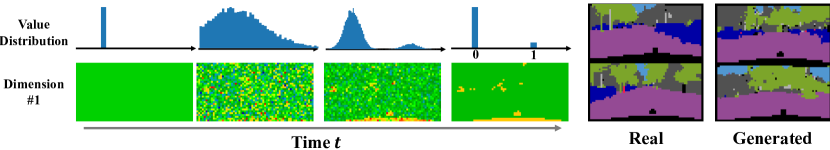
Figure 3: Results on generating categorical segmentation maps. Each pixel here an one-hot vector. Each dimension of the $\Omega$-bridge starts from a deterministic and evolve through a stochastic trajectory to converge to either $0$ or $1$. The generated samples have similar visual quality to the training data.

Generating Integer-valued Point Clouds    A feature of point clouds in 3D objects in graphics is that they tend to distribute even, especially if they are discretized from a mesh. This aspect is omitted in most existing works on point cloud generation. As a result they tend to generate non-uniform points that are unsuitable for real applications, which often involve converting back to meshes with procedures like Ball-Pivoting (Bernardini et al., 1999). We apply our method to generate point clouds that constrained on a integer grid which we show yields much more uniformly distributed points. To the best of our knowledge, we are the first work on integer-valued 3D point cloud generation.

A point cloud is a set of points $\{x_{i}\}_{i=1}^{m}$, $x_{i}\in\mathbb{R}^{3}$ in the 3D space, where $m$ refers to the number of points. We apply two variants of our method: Bridge ($\mathbb{R}^{d}$) and Bridge (Grid). Both of the bridges use the process ${\mathbb{Q}}:\mathrm{d}Z_{t}=\mathrm{d}W_{t}$ starting at $Z_{0}=0$, but on different domain $\Omega$. Bridge ($\mathbb{R}^{d}$) generates points in the continuous 3D space, i.e., $\Omega=\mathbb{R}^{3m}$. Bridge (Grid) generate points that on integer grids, $\Omega=\{1,\ldots,128\}^{3m}$. We test our method on ShapeNet (Chang et al., 2015) chair models, and compare it with Point Cloud Diffusion (PCD) (Luo and Hu, 2021a), a state-of-the-art continuous diffusion-based generative model for point clouds. The neural network $f^{\theta}$ in our methods are the same as that of PCD for fair comparison. Qualitative results and quantitative results are shown in Figure 2 and Table 1. As common practice (Luo and Hu, 2021a, b), we measure minimum matching distance (MMD), coverage score (COV) and 1-NN accuracy (1-NNA) using Chamfer Distance (CD) with the test dataset.

Methods	ELBO ($\downarrow$)	IWBO ($\downarrow$)
Uniform Dequantization Uria et al. (2013)	1.010	0.930
Variational Dequantization Ho et al. (2019)	0.334	0.315
Argmax Flow (Softplus thres.) Hoogeboom et al. (2021)	0.303	0.290
Argmax Flow (Gumbel distr.) Hoogeboom et al. (2021)	0.365	0.341
Argmax Flow (Gumbel thres.) Hoogeboom et al. (2021)	0.307	0.287
Multinomial Diffusion Hoogeboom et al. (2021)	0.305	-
Bridge-Cat. (Constant Noise)	0.844	0.707
Bridge-Cat. (Noise Decay A)	0.276	0.232
Bridge-Cat. (Noise Decay B)	0.301	0.285
Bridge-Cat. (Noise Decay C)	0.363	0.302

Table 2: Results on the CityScapes dataset.

Methods	IS ($\uparrow$)	FID ($\downarrow$)	NLL ($\downarrow$)
Discrete
D3PM uniform $L_{vb}$ Austin et al. (2021)	5.99	51.27	5.08
D3PM absorbing $L_{vb}$ Austin et al. (2021)	6.26	41.28	4.83
D3PM Gauss $L_{vb}$ Austin et al. (2021)	7.75	15.30	3.966
D3PM Gauss $L_{\lambda=0.001}$ Austin et al. (2021)	8.54	8.34	3.975
D3PM Gauss + logistic $L_{\lambda=0.001}$	8.56	7.34	3.435
Bridge-Integer (Init. A)	8.77	6.77	3.46
Bridge-Integer (Init. B)	8.68	6.91	3.35
Bridge-Integer (Init. C)	8.72	6.94	3.40

Table 3: Discrete CIFAR10 Image Generation

Generating Semantic Segmentation Maps on CityScapes

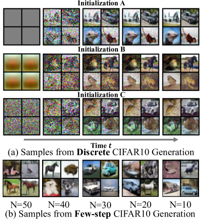
Figure 4: (a) Bridges can generate high-quality discrete samples with different initialization distribution. (b) The model can generate recognizable images even when the number of iterations is small.

We consider unconditionally generating categorical semantic segmentation maps. We represent each pixels as a one-hot categorical vector. Hence the data domain is $\Omega=\{e_{1},\ldots,e_{c}\}^{h\times w}$, where $c$ is the number of classes and $e_{i}$ is the $i$-th $c$-dimensional one-hot vector, and $h,w$ represent the height and width of the image. In CityScapes Cordts et al. (2016), $h=32,w=64,c=8$. We test a number of bridge models with ${\mathbb{Q}}:\mathrm{d}Z_{t}=\varsigma_{t}\mathrm{d}W_{t}$ starting at the uniform point $Z_{0}=1/c$, with different schedule of the diffusion coefficient $\varsigma_{t}$, including (Constant Noise): $\varsigma_{t}=1$; (Noise Decay A): $\varsigma_{t}=a\exp(-bt)$; (Noise Decay B): $\varsigma_{t}=a(1-t)$; (Noise Decay C) $\varsigma_{t}=a-a\exp(-b(1-t))$. Here $a$ and $b$ are hyper-parameters. We measure the negative log-likelihood (NLL) of the test set using the learned models. The NLL (bits-per-dimension) is estimated with evidence lower bound (ELBO) and importance weighted bound (IWBO) Burda et al. (2016), respectively. The results are shown in Figure 3 and Table 2.

Methods	$K=1000$	$K=50$	$K=40$	$K=30$	$K=20$	$K=10$
DDPM	3.37	37.96	95.79	135.23	199.22	257.78
SMLD	2.45	140.98	157.67	169.62	267.21	361.23
Bridge	9.80	18.55	19.11	21.14	24.93	34.97
Bridge (Init. C)	9.65	17.91	18.71	20.31	24.12	33.38

Table 4: Results on continuous CIFAR10 generation when varying the number of diffusion steps in both training and testing. Our method shows significant advantages in regime of small diffusion steps ($K\leq 50$).

Generating Discrete CIFAR10 Images    In this experiment, we apply three types of bridges. All of these bridges use the same output domain $\Omega=\{0,\ldots,255\}^{h\times w\times c}$, where $h,w,c$ are the height, width and number of channels of the images, respectively. We set ${\mathbb{Q}}$ to be Brownian motion with the Noise Decay A in Section 3, that is, ${\mathbb{Q}}:\mathrm{d}Z_{t}=\varsigma_{t}\mathrm{d}W_{t}$, where $\varsigma_{t}=a\exp(-bt)$. We consider different initializations of ${\mathbb{Q}}$: (Init. A) $Z_{0}={128}$; (Init. B) $Z_{0}={\hat{\mu}_{0}}$, (Init. C) $Z_{0}\sim\mathcal{N}(\hat{\mu}_{0},\hat{\sigma}_{0})$, where $\hat{\mu}_{0}$ and $\hat{\sigma}_{0}$ are the empirical mean and variance of pixels in the CIFAR10 training set. We compare with the variants of a state-of-the-art discrete diffusion model, D3PM (Austin et al., 2021). For fair comparison, we use the DDPM backbone (Ho et al., 2020) as the neural drift $f^{\theta}$ in our method, similar to D3PM. We report the Inception Score (IS) Salimans et al. (2016), Fréchet Inception Distance (FID) Heusel et al. (2017) and negative log-likelihood (NLL) of the test dataset. The results are shown in Table 3 and Figure 4.

Generating Continuous CIFAR10 Images with Few-Step Diffusion Models    In this experiment, we consider training diffusion models with very few sampling steps to generate continuous CIFAR10 images. For bridge, we use ${\mathbb{Q}}:Z_{t}=\mathrm{d}W_{t}$ initialized from $Z_{0}={0.5}$. For SMLD, we use the implementation of NCSN++ in (Song et al., 2020b). For DDPM, we use their original configuration. We use the DDPM backbone. We train the models with $K=10,20,30,40,50$ diffusion steps. Note that this is different from training with $K=1000$ steps, then sampling with fewer steps. Because in the latter case, the neural network is trained on more time steps which are unnecessary when sampling. This could hurt performance. The results are shown in Table 4 and Figure 4.

7 Conclusion and Limitations

We present a framework for learning diffusion generative models that enables both theoretical analysis and algorithmic extensions to structured data domains. It leaves a number of directions for further explorations and improvement. For example, the practical impact of the choices of the bridges ${\mathbb{Q}}$, in terms of initialization, dynamics, and noise schedule, are still not well understood and need more systematical studies. The current error analysis works in the classical finite dimensional asymptotic regime and does not consider optimization error, one direction is to extend it to high dimensional and non-asymptotic analysis and consider the training dynamics with stochastic gradient descent equipped with neural network architectures, using techniques such as neural tangent kernels.

Appendix A Appendix

A.1 Derivation of the main loss in Equation (4)

[Proof of Equation (4)] Denote by ${\mathbb{Q}}^{x}={\mathbb{Q}}(\cdot|Z_{\tau}=x)$. Note that

$$\mathcal{KL}({\mathbb{Q}}^{\Pi^{*}}~{}||~{}\mathbb{P}^{\theta}) =\mathbb{E}_{x\sim{\Pi^{*}},Z\sim{\mathbb{Q}}^{x}}\left[\log\frac{\mathrm{d}{\mathbb{Q}}^{\Pi^{*}}}{\mathrm{d}\mathbb{P}^{\theta}}(Z)\right]$$

$$=\mathbb{E}_{x\sim{\Pi^{*}},Z\sim{\mathbb{Q}}^{x}}\left[\log\frac{\mathrm{d}{\mathbb{Q}}^{x}}{\mathrm{d}\mathbb{P}^{\theta}}(Z)+\log\frac{\mathrm{d}{\mathbb{Q}}^{\Pi^{*}}}{\mathrm{d}{\mathbb{Q}}^{x}}(Z)\right]$$

$$=\mathbb{E}_{x\sim\Pi^{*}}\left[\mathcal{KL}({\mathbb{Q}}^{x}~{}||~{}\mathbb{P}^{\theta})\right]+const,$$

where $const$ denotes a constant that is independent of $\theta$. Recall that ${\mathbb{Q}}^{x}$ follows $\mathrm{d}Z_{t}=\eta^{x}(Z_{[0,t]},t)\mathrm{d}t+\sigma(Z_{t},t)\mathrm{d}W_{t}$, and $\mathbb{P}^{\theta}$ follows $\mathrm{d}Z_{t}=s^{\theta}(Z_{t},t)\mathrm{d}t+\sigma(Z_{t},t)\mathrm{d}W_{t}$. By Girsanov theorem (e.g., Lejay, 2018),

$$\mathcal{KL}({\mathbb{Q}}^{x}~{}||~{}\mathbb{P}^{\theta}) =\mathcal{KL}({\mathbb{Q}}^{x}_{0}~{}||~{}\mathbb{P}^{\theta}_{0})+\frac{1}{2}\mathbb{E}_{Z\sim{\mathbb{Q}}^{x}}\left[\int_{0}^{{T}}\left\lVert s^{\theta}(Z_{t},t)-\eta^{x}(Z_{[0,t]},t)\right\rVert^{2}_{2}\mathrm{d}t\right]$$

$$=\mathbb{E}_{Z\sim{\mathbb{Q}}^{x}}\left[-\log p_{0}^{\theta}(Z_{0})+\frac{1}{2}\int_{0}^{{T}}\left\lVert s^{\theta}(Z_{t},t)-\eta^{x}(Z_{[0,t]},t)\right\rVert^{2}_{2}\mathrm{d}t\right]+const.$$

Hence

$$L(\theta) =\mathbb{E}_{x\sim{\Pi^{*}},Z\sim{\mathbb{Q}}^{x}}\left[-\log p_{0}^{\theta}(Z_{0})+\frac{1}{2}\int_{0}^{{T}}\left\lVert s^{\theta}(Z_{t},t)-\eta^{x}(Z_{[0,t]},t)\right\rVert^{2}_{2}\mathrm{d}t\right]+const$$

$$=\mathbb{E}_{Z\sim{\mathbb{Q}}^{\Pi^{*}}}\left[-\log p_{0}^{\theta}(Z_{0})+\frac{1}{2}\int_{0}^{{T}}\left\lVert s^{\theta}(Z_{t},t)-\eta^{Z_{{T}}}(Z_{[0,t]},t)\right\rVert^{2}_{2}\mathrm{d}t\right]+const.$$

A.2 Derivation of the drift $\eta^{\Pi^{*}}$ of ${\mathbb{Q}}^{\Pi^{*}}$

Lemma A.1.

Let ${\mathbb{Q}}^{x}$ is the law of

$$\mathrm{d}Z^{x}_{t}=\eta^{x}(Z^{x}_{[0,t]},t)\mathrm{d}t+\sigma(Z^{x}_{t},t)\mathrm{d}W_{t},~{}~{}~{}Z_{0}\sim{\mathbb{Q}}^{x}_{0},$$

and ${\mathbb{Q}}^{\Pi^{*}}\coloneqq\int{\mathbb{Q}}^{x}(Z){\Pi^{*}}(\mathrm{d}x)$ for a distribution ${\Pi^{*}}$ on $\mathbb{R}^{d}$. Then ${\mathbb{Q}}^{\Pi^{*}}$ is the law of

$$\mathrm{d}Z_{t}=\eta^{\Pi^{*}}(Z_{[0,t]},t)\mathrm{d}t+\sigma(Z_{t},t)\mathrm{d}W_{t},~{}~{}~{}~{}Z_{0}\sim{\mathbb{Q}}_{0}^{\Pi^{*}},$$

where

$$\eta^{\Pi^{*}}(z_{[0,t]},t)=\mathbb{E}_{x\sim{\Pi^{*}},Z\sim{\mathbb{Q}}^{x}}[\eta^{x}(Z_{[0,t]},t)~{}|~{}Z_{[0,t]}=z_{[0,t]}], {\mathbb{Q}}^{\Pi^{*}}_{0}(\mathrm{d}z_{0})=\mathbb{E}_{x\sim{\Pi^{*}}}[{\mathbb{Q}}^{x}_{0}(\mathrm{d}z_{0})].$$

[Proof] ${\mathbb{Q}}^{\Pi^{*}}$ is the solution of the following optimization problem:

$${\mathbb{Q}}^{\Pi^{*}}=\operatorname*{arg\,min}_{\mathbb{P}}\left\{\mathcal{KL}({\mathbb{Q}}^{\Pi^{*}}~{}||~{}\mathbb{P})=\mathbb{E}_{x\sim{\Pi^{*}}}[\mathcal{KL}({\mathbb{Q}}^{x}~{}||~{}\mathbb{P})]+const\right\}.$$

By Girsanov’s Theorem (e.g., Lejay, 2018), any stochastic process $\mathbb{P}$ that has $\mathcal{KL}({\mathbb{Q}}^{x}~{}||~{}\mathbb{P})<+\infty$ (and hence is equivalent to ${\mathbb{Q}}^{x}$) has a form of $\mathrm{d}Z_{t}=\eta^{\Pi^{*}}(Z_{[0,t]},t)\mathrm{d}t+\sigma(Z_{t},t)\mathrm{d}W_{t}$ for some measurable function $\eta^{\Pi^{*}}$, and

$$\mathbb{E}_{x\sim{\Pi^{*}}}[\mathcal{KL}({\mathbb{Q}}^{x}~{}||~{}\mathbb{P})]$$

$$=\mathbb{E}_{x\sim{\Pi^{*}}}[\mathcal{KL}({\mathbb{Q}}^{x}_{0}~{}||~{}\mathbb{P}_{0})]+\mathbb{E}_{x\sim{\Pi^{*}},Z\sim{\mathbb{Q}}^{x}}\left[\frac{1}{2}\int_{0}^{{T}}\left\lVert\sigma(Z_{t},t)^{-1}(\eta^{\Pi^{*}}(Z_{[0,t]},t)-\eta^{x}(Z_{[0,t]},0))\right\rVert_{2}^{2}\right].$$

It is clear that to achieve the minimum, we need to take $\mathbb{P}_{0}(\cdot)=\mathbb{E}_{x\sim{\Pi^{*}}}[{\mathbb{Q}}_{0}^{x}(\cdot)]$ and $\eta^{\Pi^{*}}(z_{[0,t]},t)=\mathbb{E}_{x\sim{\Pi^{*}},Z\sim{\mathbb{Q}}^{x}}[\eta^{x}(Z_{[0,t]},t)~{}|~{}Z_{[0,t]}=z_{[0,t]}]$, which yields the desirable form of ${\mathbb{Q}}^{\Pi^{*}}$.

A.3 Derivation of Markovization (Proposition 2.1)

[Proof of Proposition 2.1] It is the combined result of Lemma A.2 and Lemma A.3 below.

Lemma A.2.

Let ${\mathbb{Q}}$ be a non-Markov diffusion process on $[0,{{T}}]$ of form

$${\mathbb{Q}}:~{}~{}~{}~{}~{}\mathrm{d}Z_{t}=\eta(Z_{[0,t]},t)\mathrm{d}t+\sigma(Z_{t},t)\mathrm{d}W_{t},~{}~{}~{}Z_{0}\sim{\mathbb{Q}}_{0},$$

and $\mathbb{M}=\operatorname*{arg\,min}_{\mathbb{P}\in\mathcal{M}}\mathcal{KL}({\mathbb{Q}}~{}||~{}\mathbb{P})$ be the Markovization of ${\mathbb{Q}}$, where $\mathcal{M}$ is the set of all Markov processes on $[0,{{T}}]$. Then ${\mathbb{Q}}$ is the law of

$$\mathbb{M}:~{}~{}~{}~{}~{}\mathrm{d}Z_{t}=m(Z_{t},t)\mathrm{d}t+\sigma(Z_{t},t)\mathrm{d}W_{t},~{}~{}~{}Z_{0}\sim{\mathbb{Q}}_{0},$$

where

$$m(z,t)=\mathbb{E}_{Z\sim{\mathbb{Q}}}[\eta(Z_{[0,t]},t)~{}|~{}Z_{t}=z].$$

In addition, we have ${\mathbb{Q}}_{t}=\mathbb{M}_{t}$ for all time $t\in[0,{{T}}]$.

[Proof] By Girsanov’s Theorem (e.g., Lejay, 2018), any process that has $\mathcal{KL}({\mathbb{Q}}~{}||~{}\mathbb{M})<+\infty$ (and hence is equivalent to ${\mathbb{Q}}$) has a form of $\mathrm{d}Z_{t}=m(Z_{[0,t]},t)\mathrm{d}t+\sigma(Z_{t},t)\mathrm{d}W_{t}$, where $m$ is a measurable function. Since $\mathbb{M}$ is Markov, we have $m(Z_{[0,t]},t)=m(Z_{t},t)$. Then

$$\mathcal{KL}({\mathbb{Q}}~{}||~{}\mathbb{P})=\mathcal{KL}({\mathbb{Q}}_{0}~{}||~{}\mathbb{P}_{0})+\mathbb{E}_{Z\sim{\mathbb{Q}}}\left[\frac{1}{2}\int_{0}^{{T}}\left\lVert\sigma(Z_{t},t)^{-1}(\eta(Z_{[0,t]},t)-m(Z_{t},0))\right\rVert_{2}^{2}\right].$$

It is clear that to achieve the minimum, we need to take $\mathbb{M}_{0}={\mathbb{Q}}_{0}$ and $m(z,t)=\mathbb{E}_{Z\sim{\mathbb{Q}}}[\eta(Z_{[0,t]},t)~{}|~{}Z_{t}=z]$.

To prove ${\mathbb{Q}}_{t}=\mathbb{M}_{t}$, note that by the chain rule of KL divergence:

$$\mathcal{KL}({\mathbb{Q}}~{}||~{}\mathbb{P})=\mathcal{KL}({\mathbb{Q}}_{t}~{}||~{}\mathbb{P}_{t})+\mathbb{E}_{Z_{t}\sim{\mathbb{Q}}_{t}}[\mathcal{KL}({\mathbb{Q}}(\cdot|Z_{t})~{}||~{}\mathbb{P}(\cdot|Z_{t}))],~{}~{}~{}\forall t\in[0,{{T}}].$$

As the second term $\mathbb{P}(\cdot|Z_{t})$ is independent of the choice of the marginal $\mathbb{P}_{t}$ at time $t\in[0,{{T}}]$, the optimum should be achieved by $\mathbb{M}$ only if $\mathbb{M}_{t}={\mathbb{Q}}_{t}$.

Lemma A.3.

Let

$${\mathbb{Q}}:~{}~{}~{}~{}~{}\mathrm{d}Z_{t}=\eta(Z_{[0,t]},t)\mathrm{d}t+\sigma(Z_{t},t)\mathrm{d}W_{t},~{}~{}~{}Z_{0}\sim{\mathbb{Q}}_{0}$$

$$\mathbb{M}:~{}~{}~{}~{}~{}\mathrm{d}Z_{t}=m(Z_{t},t)\mathrm{d}t+\sigma(Z_{t},t)\mathrm{d}W_{t},~{}~{}~{}Z_{0}\sim{\mathbb{Q}}_{0},$$

$$\mathbb{P}^{\theta}:~{}~{}~{}~{}~{}\mathrm{d}Z_{t}=s^{\theta}(Z_{t},t)\mathrm{d}t+\sigma(Z_{t},t)\mathrm{d}W_{t},~{}~{}~{}Z_{0}\sim\mathbb{P}^{\theta}_{0},$$

where $\mathbb{M}$ is the Markovization of ${\mathbb{Q}}$ (see Lemma A.2). Then

$$\mathcal{KL}({\mathbb{Q}}~{}||~{}\mathbb{P}^{\theta})=\mathcal{KL}({\mathbb{Q}}~{}||~{}\mathbb{M})+\mathcal{KL}(\mathbb{M}~{}||~{}\mathbb{P}^{\theta}).$$

Hence, assume there exists $\theta^{*}$ such that $\mathbb{P}^{\theta^{*}}=\mathbb{M}$ and write ${\mathcal{L}}(\theta)\coloneqq\mathcal{KL}({\mathbb{Q}}~{}||~{}\mathbb{P}^{\theta}).$ We have

$$\mathcal{KL}(\mathbb{Q}_{{T}}~{}||~{}\mathbb{P}^{\theta}_{{T}})=\mathcal{KL}(\mathbb{M}_{{T}}~{}||~{}\mathbb{P}^{\theta}_{{T}})\leq\mathcal{KL}(\mathbb{M}~{}||~{}\mathbb{P}^{\theta})={\mathcal{L}}(\theta)-{\mathcal{L}}(\theta^{*}).$$

[Proof] Note that

$$\mathcal{KL}(\mathbb{M}~{}||~{}\mathbb{P}^{\theta})$$

$$=\mathcal{KL}(\mathbb{M}_{0}~{}||~{}\mathbb{P}_{0}^{\theta})+\frac{1}{2}\mathbb{E}_{Z_{t}\sim\mathbb{M}_{t}}\left[\int_{0}^{{T}}\left\lVert\sigma(Z_{t},t)^{-1}(s^{\theta}(Z_{t},t)-m(Z_{t},t))\right\rVert_{2}^{2}\right]\mathrm{d}t$$

$$=\mathcal{KL}(\mathbb{M}_{0}~{}||~{}\mathbb{P}_{0}^{\theta})+\frac{1}{2}\int_{0}^{{T}}\mathbb{E}_{Z_{t}\sim\mathbb{M}_{t}}\left[\left\lVert\sigma(Z_{t},t)^{-1}(s^{\theta}(Z_{t},t)-m(Z_{t},t))\right\rVert_{2}^{2}\right]\mathrm{d}t$$

$$=\mathcal{KL}({\mathbb{Q}}_{0}~{}||~{}\mathbb{P}_{0}^{\theta})+\frac{1}{2}\int_{0}^{{T}}\mathbb{E}_{Z_{t}\sim{\mathbb{Q}}_{t}}\left[\left\lVert\sigma(Z_{t},t)^{-1}(s^{\theta}(Z_{t},t)-m(Z_{t},t))\right\rVert_{2}^{2}\right]\mathrm{d}t~{}~{}~{}~{}~{}~{}~{}\text{{//${\mathbb{Q}}_{t}=\mathbb{M}_{t}~{}~{}\forall t$}}$$

$$=\mathcal{KL}({\mathbb{Q}}_{0}~{}||~{}\mathbb{P}_{0}^{\theta})+\mathbb{E}_{Z\sim{\mathbb{Q}}}\left[\frac{1}{2}\int_{0}^{{T}}\left\lVert\sigma(Z_{t},t)^{-1}(s^{\theta}(Z_{t},t)-m(Z_{t},t))\right\rVert_{2}^{2}\mathrm{d}t\right]$$

$$=\mathcal{KL}({\mathbb{Q}}_{0}~{}||~{}\mathbb{P}_{0}^{\theta})+\frac{1}{2}\left\lVert s^{\theta}-m\right\rVert_{{\mathbb{Q}},\sigma}^{2},$$

where we define $\left\lVert f\right\rVert_{{\mathbb{Q}},\sigma}^{2}=\mathbb{E}_{Z\sim{\mathbb{Q}}}\left[\frac{1}{2}\int_{0}^{{T}}\left\lVert\sigma(Z_{t},t)^{-1}f(Z_{t},t)\right\rVert_{2}^{2}\mathrm{d}t\right].$

On the other hand,

$$\mathcal{KL}({\mathbb{Q}}~{}||~{}\mathbb{P}^{\theta}) =\mathcal{KL}({\mathbb{Q}}_{0}~{}||~{}\mathbb{P}_{0}^{\theta})+\mathbb{E}_{Z\sim{\mathbb{Q}}}\left[\frac{1}{2}\int_{0}^{{T}}\left\lVert\sigma(Z_{t},t)^{-1}(s^{\theta}(Z_{t},0))-\eta(Z_{[0,t]},t)\right\rVert_{2}^{2}\mathrm{d}t\right]$$

$$=\mathcal{KL}({\mathbb{Q}}_{0}~{}||~{}\mathbb{P}_{0}^{\theta})+\frac{1}{2}\left\lVert s^{\theta}-\eta\right\rVert_{{\mathbb{Q}},\sigma}^{2}$$

$$\mathcal{KL}({\mathbb{Q}}~{}||~{}\mathbb{M}) =\mathbb{E}_{Z\sim{\mathbb{Q}}}\left[\frac{1}{2}\int_{0}^{{T}}\left\lVert\sigma(Z_{t},t)^{-1}(\eta(Z_{[0,t]},t)-m(Z_{t},0))\right\rVert_{2}^{2}\mathrm{d}t\right]$$

$$=\frac{1}{2}\left\lVert\eta-m\right\rVert_{{\mathbb{Q}},\sigma}^{2}.$$

Using Lemma A.4 with $a(z)=\sigma(z,t)^{-1}s^{\theta}(z,t)$, and $b(z_{[0,t]})=\sigma(z,t)^{-1}\eta(z_{[0,t]},t)$, we have the following bias-variance decomposition:

$$\left\lVert\eta-s^{\theta}\right\rVert_{{\mathbb{Q}},\sigma}^{2}=\left\lVert s^{\theta}-m\right\rVert_{{\mathbb{Q}},\sigma}^{2}+\left\lVert\eta-m\right\rVert_{{\mathbb{Q}},\sigma}^{2}.$$

Hence, $\mathcal{KL}({\mathbb{Q}}~{}||~{}\mathbb{P}^{\theta})=\mathcal{KL}(\mathbb{M}~{}||~{}\mathbb{P}^{\theta})+\mathcal{KL}({\mathbb{Q}}~{}||~{}\mathbb{M})$.

Finally, $\mathcal{KL}(M_{{T}}~{}||~{}\mathbb{P}_{{T}}^{\theta})\leq\mathcal{KL}(\mathbb{M}~{}||~{}\mathbb{P}^{\theta})$ is the direct result of the following factorization of KL divergence:

$$\mathcal{KL}(\mathbb{M}~{}||~{}\mathbb{P}^{\theta})=\mathcal{KL}(\mathbb{M}_{{T}}~{}||~{}\mathbb{P}_{{T}}^{\theta})+\mathbb{E}_{x\sim\mathbb{M}_{{T}}}\left[\mathcal{KL}(\mathbb{M}_{{T}}(\cdot|Z_{{T}}=x)~{}||~{}\mathbb{P}_{{T}}^{\theta}(\cdot|Z_{{T}}=x))\right].$$

Lemma A.4.

Let $(X,Y)$ be a random variable and $a(x)$, $b(x,y)$ are square integral functions. Let $m(x)=\mathbb{E}[b(X,Y)~{}|~{}X=x]$. We have

$$\mathbb{E}[\left\lVert a(X)-b(X,Y)\right\rVert^{2}_{2}]=\mathbb{E}[\left\lVert a(X)-m(X)\right\rVert^{2}_{2}]+\mathbb{E}[\left\lVert b(X,Y)-m(X)\right\rVert^{2}_{2}].$$

[Proof]

$$\mathbb{E}[\left\lVert a(X)-b(X,Y)\right\rVert^{2}_{2}] =\mathbb{E}[\left\lVert a(X)-m(X)+m(X)-b(X,Y)\right\rVert^{2}_{2}]$$

$$=\mathbb{E}[\left\lVert a(X)-m(X)\right\rVert^{2}_{2}]+\mathbb{E}[\left\lVert m(X)-b(X,Y)\right\rVert^{2}_{2}]+2\Delta,$$

where

$$\Delta =\mathbb{E}[(a(X)-m(X))^{\top}(m(X)-b(X,Y))]]$$

$$=\mathbb{E}[(a(X)-m(X))^{\top}\mathbb{E}[(m(X)-b(X,Y))|X]]$$

$$=\mathbb{E}[(a(X)-m(X))^{\top}(m(X)-m(X))]=0.$$

A.4 SMLD and DDPM as bridges with uninformative initialization

We show that methods like SMLD and DDPM that specify ${\mathbb{Q}}^{x}$ as a time reversed O-U process $Z^{x}_{t}=\tilde{Z}^{x}_{{{T}}-t}$ with $\mathrm{d}\tilde{Z}^{x}_{t}=-\alpha_{{{T}}-t}\tilde{Z}^{x}_{t}\mathrm{d}t+\varsigma_{{{T}}-t}\mathrm{d}\tilde{W}_{t}$ and $\tilde{Z}_{0}=x$ can be viewed as taking ${\mathbb{Q}}^{x}={\mathbb{Q}}(\cdot|Z_{{T}}=x)$ with ${\mathbb{Q}}$ the law of $\mathrm{d}Z_{t}=\alpha_{t}Z_{t}\mathrm{d}t+\varsigma_{t}\mathrm{d}t$ initialized from $\mathcal{N}(0,v)$ with $v\to+\infty$. This is made concrete in the following result.

Proposition A.5.

Let ${\mathbb{Q}}^{x}$ be the law of $Z^{x}_{t}=\tilde{Z}^{x}_{{{T}}-t}$ following $\mathrm{d}\tilde{Z}^{x}_{t}=-\alpha_{{{T}}-t}\tilde{Z}^{x}_{t}\mathrm{d}t+\varsigma_{{{T}}-t}\mathrm{d}\tilde{W}_{t}$ with $\tilde{Z}_{0}=x$. Assume $\sup_{t\in[0,T]}\{\alpha_{t},\varsigma_{t}\}<\infty$. Let ${\mathbb{Q}}_{v}:=\mathrm{Ito}(\{\alpha_{t}\},\{\beta_{t}\},\mathcal{N}(0,v))$ be the law of $\mathrm{d}Z_{t}=\alpha_{t}Z_{t}\mathrm{d}t+\varsigma_{t}\mathrm{d}W_{t}$ starting from $Z_{0}\sim\mathcal{N}(0,v)$, where $v$ is the variance of the initial distribution. Then we have ${\mathbb{Q}}^{x}=\lim_{v\to+\infty}{\mathbb{Q}}_{v}(\cdot|Z_{{T}}=x)$, where the limit denotes weak convergence.

[Proof] Let ${\mathbb{Q}}_{v}$ be the law of the O-U process $\mathrm{d}Z_{t}=\alpha_{t}Z_{t}\mathrm{d}t+\varsigma_{t}\mathrm{d}W_{t}$ initialized at $Z_{0}\sim\mathcal{N}(\mu_{0},v)$. Its solution is

$$Z_{t}=\mu_{t|0}Z_{0}+\int_{0}^{t}\mu_{t|s}\varsigma_{s}\mathrm{d}B_{s}\sim\mathcal{N}(\alpha_{t|0}\mu_{0},~{}\alpha_{t|0}^{2}v+\beta_{t|0}),$$

where we define

$$\alpha_{t|s}=\exp\left(\int_{s}^{t}\alpha_{r}\mathrm{d}r\right), \beta_{t|s}=\int_{s}^{t}\alpha_{t|r}^{2}\varsigma_{r}^{2}\mathrm{d}r, \forall 0\leq s\leq t\leq T.$$

Using the time reversal formula Anderson (1982), the time-reversed process $\tilde{Z}_{t}=Z_{T-t}$ follows

$$\mathrm{d}\tilde{Z}_{t}=\left(-\alpha_{{{T}}-t}\tilde{Z}_{t}+r(\tilde{Z}_{t},t)\right)\mathrm{d}t+\varsigma_{{{T}}-t}\mathrm{d}\tilde{W}_{t}, r(\tilde{Z}_{t},t)=\varsigma_{{{T}}-t}^{2}\frac{\alpha_{{{T}}-t|0}\mu_{0}-\tilde{Z}_{t}}{\alpha_{{{T}}-t|0}^{2}v+\beta_{{{T}}-t|0}},$$

where $\tilde{W}_{t}$ is a standard Brownian motion. Taking $v\to+\infty$, the extra drift term due to the time reversion is vanished, and hence we get the follow process in the limit:

$$\mathrm{d}\tilde{Z}_{t}=-\alpha_{{{T}}-t}\mathrm{d}t+\varsigma_{{{T}}-t}\mathrm{d}\tilde{W}_{t}.$$

This is directly reverting $\mathrm{d}Z_{t}=\alpha_{t}\mathrm{d}t+\varsigma_{t}\mathrm{d}W_{t}$ without introducing the extra term in the time reversal formula.

A.5 Markov and Reciprocal Properties of ${\mathbb{Q}}^{\Pi^{*}}$

[Proof of Proposition 3.3] This is an obvious result. We have ${\mathbb{Q}}^{z_{0},x}(Z_{{T}}=x)=1$ by the definition of conditioned processes. Hence ${\mathbb{Q}}^{x}(Z_{{T}}=x)=\int{\mathbb{Q}}^{z_{0},x}(Z_{{T}}=x)\mu(\mathrm{d}z_{0}~{}|~{}x)=\int\mu(\mathrm{d}z_{0}~{}|~{}x)=1$.

Proposition A.6.

Assume ${\mathbb{Q}}^{x}={\mathbb{Q}}(\cdot~{}|~{}Z_{{T}}=x)$ and $\pi^{*}(z)\coloneqq\frac{\mathrm{d}{\Pi^{*}}}{\mathrm{d}{\mathbb{Q}}_{{T}}}(z)$ exists and is positive everywhere. Then ${\mathbb{Q}}^{\Pi^{*}}$ is Markov, iff ${\mathbb{Q}}$ is Markov.

[Proof] If ${\mathbb{Q}}^{x}={\mathbb{Q}}(\cdot~{}|~{}Z_{{T}}=x)$, we have from the definition of ${\mathbb{Q}}^{\Pi^{*}}$:

$${\mathbb{Q}}^{\Pi^{*}}(Z)={\mathbb{Q}}(Z|Z_{{T}}){\Pi^{*}}(Z_{{T}})={\mathbb{Q}}(Z)\pi^{*}(Z_{{T}}),$$

where $\pi^{*}(Z_{{T}})=\frac{\mathrm{d}{\Pi^{*}}}{\mathrm{d}{\mathbb{Q}}_{{T}}}(Z_{{T}}).$ Therefore, ${\mathbb{Q}}^{\Pi^{*}}$ is obtained by multiplying a positive factor $\pi^{*}(Z_{{T}})$ on the terminal state $Z_{{T}}$ of ${\mathbb{Q}}$. Hence ${\mathbb{Q}}^{\Pi^{*}}$ has the same Markov structure as that of ${\mathbb{Q}}$.

[Proof of Proposition 3.4] When taking ${\mathbb{Q}}^{x}$ to be the dynamics (11) initialized from $Z_{0}\sim\mu_{0}=\mathcal{N}(0,v_{0})$, we have ${\mathbb{Q}}^{x}=\int\mu_{0}(\mathrm{d}z_{0})\tilde{\mathbb{Q}}^{z_{0},x}$, where $\tilde{\mathbb{Q}}^{z_{0},x}=\tilde{\mathbb{Q}}(\cdot|Z_{0}=z_{0},Z_{{T}}=x)$ with $\tilde{\mathbb{Q}}$ following Brownian motion $\mathrm{d}Z_{t}=\mathrm{d}W_{t}$. Hence, we can write ${\mathbb{Q}}^{\Pi^{*}}(\mathrm{d}Z)=\tilde{\mathbb{Q}}(\mathrm{d}Z)r(Z_{0},Z_{{T}})$, where $r(z_{0},z_{{T}})=\frac{\mathrm{d}\mu_{0}\otimes{\Pi^{*}}}{\mathrm{d}\tilde{\mathbb{Q}}_{0,{{T}}}}(z_{0},z_{{T}}).$ From Léonard et al. (2014), ${\mathbb{Q}}^{\Pi^{*}}$ is Markov iff $r(x,z_{0})=f(x)g(z_{0})$ for some $f$ and $g$, which is not the case except the degenerated case ($v_{0}=0$ and $v_{0}=+\infty$) because $\tilde{\mathbb{Q}}_{0,1}$ is not factorized.

On the other hand, when $v_{0}=0$, we have that ${\mathbb{Q}}^{x}={\mathbb{Q}}(\cdot|Z_{{T}}=x)$ is the standard Brownian bridge and hence ${\mathbb{Q}}^{\Pi^{*}}$ is Markov following Proposition A.6. When $v_{0}=+\infty$, as the case of SMLD, ${\mathbb{Q}}^{\Pi^{*}}$ is the law of $Z_{t}=\tilde{Z}_{{{T}}-t}$ with $\mathrm{d}\tilde{Z}_{t}=\mathrm{d}W_{t}$ and $\tilde{Z}_{0}\sim{\Pi^{*}}$, which is also Markov.

[Proof of Proposition 3.6] Note that

$${\mathbb{Q}}^{\Pi^{*}}(\cdot)=\int\pi(\mathrm{d}x){\mathbb{Q}}^{x}(\cdot)=\int\pi(\mathrm{d}x)\mu(\mathrm{d}z_{0}~{}|~{}x)\tilde{\mathbb{Q}}^{z_{0},x}(\cdot).$$

Hence if $\tilde{\mathbb{Q}}$ is Markov, ${\mathbb{Q}}^{\Pi^{*}}$ is reciprocal by Definition 3.5.

On the other hand, if ${\mathbb{Q}}^{\Pi^{*}}$ is reciprocal, we have ${\mathbb{Q}}^{\Pi^{*}}(\cdot)=\int\mathbb{M}^{z_{0},x}(\cdot)\mu(\mathrm{d}z_{0},\mathrm{d}x)$ for some Markov process $\mathbb{M}$ and probability measure $\mu$ on $\Omega\times\Omega$. In this case, we have ${\mathbb{Q}}^{x}(\cdot)={\mathbb{Q}}^{\Pi^{*}}(\cdot|Z_{{T}}=x)=\int\mathbb{M}^{z_{0},x}(\cdot)\mu(\mathrm{d}z_{0}~{}|~{}x)$, assuming it exits.

A.6 Condition for $\Omega$-bridges

Proposition A.7.

For any ${\mathbb{Q}}^{\Omega}$ following $\mathrm{d}Z_{t}=\eta^{\Omega}(Z_{t},t)\mathrm{d}t+\mathrm{d}W_{t}$ that is an $\Omega$-bridge, the $\mathbb{P}^{\theta}$ in (12) is also an $\Omega$-bridge if $\mathbb{E}_{Z\sim{\mathbb{Q}}^{\Omega}}[\int_{0}^{{T}}\left\lVert f^{\theta}(Z_{t},t)\right\rVert_{2}^{2}\mathrm{d}t]<+\infty$ and $\mathcal{KL}({\mathbb{Q}}^{\Omega}_{0}~{}||~{}\mathbb{P}^{\theta}_{0})<+\infty$.

[Proof of Proposition A.7] We know that

$$\mathcal{KL}({\mathbb{Q}}^{\Omega}~{}||\mathbb{P}^{\theta})=\mathcal{KL}({\mathbb{Q}}^{\Omega}_{0}~{}||~{}\mathbb{P}^{\theta}_{0})+\frac{1}{2}\mathbb{E}_{Z\sim{\mathbb{Q}}^{\Omega}}\left[\int_{0}^{{T}}\left\lVert f^{\theta}(Z_{t},t)\right\rVert_{2}^{2}\mathrm{d}t\right]<+\infty.$$

This means that ${\mathbb{Q}}^{\Omega}$ and $\mathbb{P}^{\theta}$ are absolutely continuous to each other, and hence have the same support. Therefore, ${\mathbb{Q}}^{\Omega}(Z_{{T}}\in\Omega)=1$ implies that $\mathbb{P}^{\theta}(Z_{{T}}\in\Omega)=1$.

A.7 Examples of $\Omega$-Bridges

If $\Omega$ is a product space, the integration can be factorized into one-dimensional integrals. So it is sufficient to focus on 1D case.

If $\Omega$ is a discrete set, say $\Omega=\{e_{1}\ldots,e_{K}\}$, we have

$$\eta_{\mathrm{bb},\varsigma}^{\Omega}(z,t) =\varsigma_{t}^{2}\frac{1}{\sum_{k=1}^{K}\omega(e_{k},z,t)}\sum_{k=1}^{K}\omega(e_{k},z,t)\frac{e_{k}-z}{\beta_{{T}}-\beta_{t}}$$

$$=\varsigma_{t}^{2}\nabla_{z}\log\sum_{k=1}^{K}\omega(e_{k},z,t),$$

where

$$\omega(e_{k},z,t)=\exp\left(-\frac{\left\lVert z-e_{k}\right\rVert^{2}}{2(\beta_{{T}}-\beta_{t})}\right).$$

If $\Omega=[a,b]$, we have

$$\eta^{\Omega}_{\mathrm{bb},\varsigma}(z,t) =\varsigma_{t}^{2}\frac{1}{\int_{a}^{b}\omega(e,z,t)}\int_{a}^{b}\omega(e,z,t)\frac{e-z}{\beta_{{T}}-\beta_{t}}\mathrm{d}e$$

$$=\varsigma_{t}^{2}\nabla_{z}\log\int_{a}^{b}\omega(e,z,t)\mathrm{d}e$$

$$=\varsigma_{t}^{2}\nabla_{z}\log\left(F(\frac{z-a}{\sqrt{\beta_{{T}}-\beta_{t}}})-F(\frac{z-b}{\sqrt{\beta_{{T}}-\beta_{t}}})\right),$$

where $F$ is the standard Gaussian CDF.

A.8 Time-Discretization Error Analysis (Proposition 4.1)

Proposition A.8.

Assume $\Omega=\mathbb{R}^{d}$ and $\sigma(z,t)=\sigma(t)$ is state-independent and $\sigma(t)>c>0$, $\forall t\in[0,{{T}}]$. Take the uniform time grid $\tau^{\mathrm{unif}}\coloneqq\{i\epsilon\}_{i=0}^{K}$ with step size $\epsilon={{T}}/K$ in the sampling step (14). Let ${\mathcal{L}}_{\epsilon}(\theta)=\mathbb{E}_{Z\sim{\mathbb{Q}}^{\Pi^{*}}}[\ell_{\epsilon}(\theta;Z)]$ with

$$\ell_{\epsilon}(\theta,Z_{t})=-\log p_{0}^{\theta}(Z_{0})+\frac{1}{2K}\sum_{k=1}^{K}\left\lVert\sigma_{k}^{-1}(s^{\theta}(Z_{{t_{k}}},{t_{k}})-\eta^{Z_{{T}}}(Z_{[0,{t_{k}}]},{t_{k}}))\right\rVert^{2}_{2},$$

where $\epsilon>0$ is a step size with ${{T}}=K\epsilon$ and ${t_{k}}=(k-1)\epsilon$, and $\sigma_{k}^{2}\coloneqq(t_{k+1}-{t_{k}})^{-1}\int_{{t_{k}}}^{t_{k+1}}\sigma(t)^{2}\mathrm{d}t$. Let $\mathbb{P}^{\theta,\epsilon}_{{T}}$ be the distribution of the sample $\hat{Z}_{{T}}$ resulting from the following Euler method:

$$\hat{Z}_{t_{k+1}}=\hat{Z}_{t_{k}}+\epsilon s^{\theta}(Z_{t_{k}},t_{k})+\sqrt{\epsilon}\sigma_{k}\xi_{k},$$

where $\xi_{k}\sim\mathcal{N}(0,I_{d})$ is the standard Gaussian noise in $\mathbb{R}^{d}$. Let $\theta^{*}$ be an optimal parameter satisfying (5). Assume $C_{0}\coloneqq\sup_{z,t}\left(\left\lVert s^{\theta^{*}}(z,t)\right\rVert^{2}/(1+\left\lVert z\right\rVert^{2}),~{}\mathrm{tr}(\sigma^{2}(z,t)),~{}\mathbb{E}_{\mathbb{P}^{\theta^{*}}}[\left\lVert Z_{0}\right\rVert^{2}]\right)<+\infty$, and $s^{\theta^{*}}$ satisfies $\left\lVert s^{\theta^{*}}(z,t)-s^{\theta^{*}}(z^{\prime},t^{\prime})\right\rVert^{2}_{2}\leq L\left(\left\lVert z-z^{\prime}\right\rVert^{2}+\left\lvert t-t^{\prime}\right\rvert\right)$ for $\forall z,z^{\prime}\in\mathbb{R}^{d}$ and $t,t^{\prime}\in[0,{{T}}]$. Then we have

$$\sqrt{\mathcal{KL}({\Pi^{*}}~{}||~{}\mathbb{P}^{\theta,\epsilon}_{{T}})}\leq\sqrt{{\mathcal{L}}_{\epsilon}(\theta)-{\mathcal{L}}_{\epsilon}(\theta^{*})}+{O}{\left(\sqrt{\epsilon}\right)}.$$

[Proof of Proposition 4.1] This is the result of Lemma A.9 below by noting that the $\hat{}\mathbb{P}^{\theta}$ there is equivalent to the Euler method above, and ${\mathcal{L}}_{\epsilon}(\theta)-{\mathcal{L}}_{\epsilon}(\theta^{*})\leq\tilde{\mathcal{L}}_{\epsilon}(\theta)-\tilde{\mathcal{L}}_{\epsilon}(\theta^{*})$ (because $\sigma_{k}^{-2}=((t_{k+1}-t_{k})^{-1}\int_{{t_{k}}}^{t_{k+1}}\sigma(t)^{2})^{-1}\leq(t_{k+1}-t_{k})^{-1}\int_{{t_{k}}}^{t_{k+1}}\sigma(t)^{-2}$).

Lemma A.9.

Let $h$ be a step size and $\epsilon=T/K$ for a positive integer $K$. For each $t\in[0,\infty)$, denote by $\lfloor t\rfloor_{\epsilon}=\max(\{k\epsilon\colon k\in\mathbb{N}\}\cap[0,t]$). Assume

$${\mathbb{Q}}^{\Pi^{*}}:~{}~{}~{}~{}~{}\mathrm{d}Z_{t}=\eta^{{\Pi^{*}}}(Z_{[0,t]},t)\mathrm{d}t+\sigma(Z_{t},t)\mathrm{d}W_{t},~{}~{}~{}Z_{0}\sim{\mathbb{Q}}_{0}$$

$$\mathbb{P}^{\theta^{*}}:~{}~{}~{}~{}~{}\mathrm{d}Z_{t}=s^{\theta^{*}}(Z_{t},t)\mathrm{d}t+\sigma(Z_{t},t)\mathrm{d}W_{t},~{}~{}~{}Z_{0}\sim{\mathbb{Q}}_{0},$$

$$\mathbb{P}^{\theta}:~{}~{}~{}~{}~{}\mathrm{d}Z_{t}=s^{\theta}(Z_{t},t)\mathrm{d}t+\sigma(Z_{t},t)\mathrm{d}W_{t},~{}~{}~{}Z_{0}\sim\mathbb{P}^{\theta}_{0}$$

$$\hat{}\mathbb{P}^{\theta}:~{}~{}~{}~{}~{}\mathrm{d}Z_{t}=s^{\theta}(Z_{\lfloor t\rfloor_{\epsilon}},t)\mathrm{d}t+\sigma(Z_{t},t)\mathrm{d}W_{t},~{}~{}~{}Z_{0}\sim\mathbb{P}^{\theta}_{0},$$

where $\mathbb{P}^{\theta^{*}}$ is the Markovianization of ${\mathbb{Q}}^{\Pi^{*}}$, and $\hat{}\mathbb{P}^{\theta}$ is a discretized version of $\mathbb{P}^{\theta}$. Define

$$\tilde{\mathcal{L}}_{\epsilon}(\theta)=\mathbb{E}_{{\mathbb{Q}}^{\Pi^{*}}}\left[-\log p_{0}^{\theta}(Z_{0})+\frac{1}{2}\int_{0}^{{T}}\left\lVert\sigma^{-1}(Z_{t},t)(s^{\theta}(Z_{\lfloor t\rfloor_{\epsilon}},\lfloor t\rfloor_{\epsilon})-\eta^{Z_{{T}}}(Z_{[0,\lfloor t\rfloor_{\epsilon}]},\lfloor t\rfloor_{\epsilon}))\right\rVert^{2}\mathrm{d}t\right].$$

Assume the conditions of Lemma A.13 holds for $\mathbb{P}^{\theta^{*}}$, and $\sigma(z,t)\geq c>0$ for all $z,t$, and $s^{\theta^{*}}$ satisfies $\left\lVert s^{\theta^{*}}(z,t)-s^{\theta^{*}}(z^{\prime},t^{\prime})\right\rVert^{2}_{2}\leq L\left(\left\lVert z-z^{\prime}\right\rVert^{2}+\left\lvert t-t^{\prime}\right\rvert\right)$ for $\forall z,z^{\prime}\in\mathbb{R}^{d}$ and $t,t^{\prime}\in[0,{{T}}]$. Then

$$\sqrt{\mathcal{KL}(\mathbb{P}^{\theta^{*}}~{}||~{}\hat{}\mathbb{P}^{\theta})}\leq\sqrt{\tilde{\mathcal{L}}_{\epsilon}(\theta)-\tilde{\mathcal{L}}_{\epsilon}(\theta^{*})}+C\sqrt{\epsilon},$$

where $C$ is a constant that is independent of $\epsilon$.

[Proof] Define $\left\lVert f\right\rVert_{{\mathbb{Q}},\sigma}^{2}=\mathbb{E}_{Z\sim{\mathbb{Q}}}[\int_{0}^{T}\left\lVert\sigma(Z,t)f(Z,t)\right\rVert^{2}]$ for convenient notation. Let $s^{\theta}_{\epsilon}(Z,t)=s^{\theta}(Z_{\lfloor t\rfloor_{\epsilon}},\lfloor t\rfloor_{\epsilon})$, and $\eta_{\epsilon}=\eta^{Z_{T}}(Z_{[0,\lfloor t\rfloor_{\epsilon}]},\lfloor t\rfloor_{\epsilon})$.

$$\mathcal{KL}(\mathbb{P}^{\theta^{*}}~{}||~{}\hat{}\mathbb{P}^{\theta})$$

$$=\mathcal{KL}(\mathbb{P}^{\theta^{*}}_{0}~{}||~{}\hat{}\mathbb{P}^{\theta}_{0})+\frac{1}{2}\left\lVert s^{\theta^{*}}-s^{\theta}_{\epsilon}\right\rVert^{2}$$

$$\leq\mathcal{KL}(\mathbb{P}^{\theta^{*}}_{0}~{}||~{}\mathbb{P}^{\theta}_{0})+\frac{1}{2}\left((1+\omega)\left\lVert s^{\theta}_{\epsilon}-s^{\theta^{*}}_{\epsilon}\right\rVert^{2}_{\mathbb{P}^{\theta^{*}},\sigma}+(1+1/\omega)\left\lVert s^{\theta^{*}}-s^{\theta^{*}}_{\epsilon}\right\rVert^{2}_{\mathbb{P}^{\theta^{*}},\sigma}\right)$$

$$\coloneqq(1+\omega)I_{1}+(1+1/\omega)I_{2},$$

where $\omega>0$ is any positive number and

$$I_{1} \coloneqq\frac{1}{1+\omega}\mathcal{KL}(\mathbb{P}^{\theta^{*}}_{0}~{}||~{}\mathbb{P}^{\theta}_{0})+\frac{1}{2}\left\lVert s^{\theta}_{\epsilon}-s^{\theta^{*}}_{\epsilon}\right\rVert^{2}_{\mathbb{P}^{\theta^{*}},\sigma}$$

$$=\frac{1}{1+\omega}\mathcal{KL}(\mathbb{P}^{\theta^{*}}_{0}~{}||~{}\mathbb{P}^{\theta}_{0})+\frac{1}{2}\left\lVert s^{\theta}_{\epsilon}-s^{\theta^{*}}_{\epsilon}\right\rVert^{2}_{{\mathbb{Q}}^{\Pi^{*}},\sigma}$$

$$\leq\mathcal{KL}(\mathbb{P}^{\theta^{*}}_{0}~{}||~{}\mathbb{P}^{\theta}_{0})+\frac{1}{2}\left\lVert s^{\theta}_{\epsilon}-s^{\theta^{*}}_{\epsilon}\right\rVert^{2}_{{\mathbb{Q}}^{\Pi^{*}},\sigma}$$

$$\leq\mathcal{KL}(\mathbb{P}^{\theta^{*}}_{0}~{}||~{}\mathbb{P}^{\theta}_{0})+\frac{1}{2}\left(\left\lVert s^{\theta}_{\epsilon}-\eta^{Z_{{T}}}_{\epsilon}\right\rVert^{2}_{{\mathbb{Q}}^{\Pi^{*}},\sigma}-\left\lVert s^{\theta^{*}}_{\epsilon}-\eta^{Z_{{T}}}_{\epsilon}\right\rVert^{2}_{{\mathbb{Q}}^{\Pi^{*}},\sigma}\right)~{}~{}~{}~{}~{}~{}~{}\text{{//Lemma~{}\ref{lem:vb}}}$$

$$=\tilde{\mathcal{L}}_{\epsilon}(\theta)-\tilde{\mathcal{L}}_{\epsilon}(\theta^{*}),$$

and

$$I_{2} \coloneqq\frac{1}{2}\left\lVert s^{{\theta^{*}}}-s^{\theta^{*}}_{\epsilon}\right\rVert_{\mathbb{P}^{\theta^{*}},\sigma}^{2}$$

$$\leq\frac{L}{2}\mathbb{E}_{\mathbb{P}^{\theta^{*}}}\left[\int_{0}^{{T}}\sigma^{-2}(Z_{t},t)\left(\left\lVert Z_{t}-Z_{\lfloor t\rfloor_{\epsilon}}\right\rVert^{2}+(t-\lfloor t\rfloor_{\epsilon})\right)\mathrm{d}t\right]$$

$$\leq\frac{L}{2c^{2}}\mathbb{E}_{\mathbb{P}^{\theta^{*}}}\left[\int_{0}^{{T}}((Z_{t}-Z_{\lfloor t\rfloor_{\epsilon}})^{2}+(t-\lfloor t\rfloor_{\epsilon}))\mathrm{d}t\right]$$

$$\leq\frac{L}{2c^{2}}\left(C_{\mathbb{P}^{\theta^{*}}}+1\right)\int_{0}^{{T}}(t-\lfloor t\rfloor_{\epsilon})\mathrm{d}t~{}~{}~{}~{}~{}~{}~{}\text{{//Lemma~{}\ref{lem:bound}}}$$

$$=\frac{L}{2c^{2}}\left(C_{\mathbb{P}^{\theta^{*}}}+1\right)\frac{{{T}}\epsilon}{2}.~{}~{}~{}~{}~{}~{}~{}\text{{//Lemma~{}\ref{lem:tth},}}$$

where $C_{\mathbb{P}^{\theta^{*}}}$ is a constant depending on $\mathbb{P}^{\theta^{*}}$ that comes from Lemma A.13. Hence

$$\mathcal{KL}(\mathbb{P}^{\theta^{*}}~{}||~{}\hat{}\mathbb{P}^{\theta}) \leq\inf_{\omega\geq 0}(1+\omega)I_{1}+(1+1/\omega)I_{2}$$

$$=(\sqrt{I_{1}}+\sqrt{I_{2}})^{2}$$

$$\leq\left(\sqrt{\tilde{\mathcal{L}}_{\epsilon}(\theta)-\tilde{\mathcal{L}}_{\epsilon}(\theta^{*})}+\frac{1}{2}\sqrt{\frac{L}{c^{2}}\left(C_{\mathbb{P}^{\theta^{*}}}+1\right){{T}}\epsilon}\right).$$

This completes the proof.

Lemma A.10.

For any $a,b\in\mathbb{R}^{d}$, and $\omega\geq 0$,

$$\left\lVert a+b\right\rVert^{2}_{2}\leq(1+\omega)\left\lVert a\right\rVert^{2}_{2}+(1+1/\omega)\left\lVert b\right\rVert_{2}^{2}.$$

[Proof]

$$(1+\omega)\left\lVert a\right\rVert^{2}_{2}+(1+1/\omega)\left\lVert b\right\rVert_{2}^{2}\geq\left\lVert a\right\rVert_{2}^{2}+\left\lVert b\right\rVert_{2}^{2}+2a^{\top}b=\left\lVert a+b\right\rVert^{2}_{2}$$

Lemma A.11.

Assume ${{T}}\geq 0$, $\epsilon\geq 0$ and ${{T}}/\epsilon\in\mathbb{N}$. We have

$$\int_{0}^{{T}}(t-\lfloor t\rfloor_{\epsilon})\mathrm{d}t=\frac{{{T}}\epsilon}{2}.$$

[Proof]

$$\int_{0}^{{T}}(t-\lfloor t\rfloor_{\epsilon})\mathrm{d}t =\sum_{k=0}^{K-1}\int_{0}^{\epsilon}(hk+x-hk)\mathrm{d}x$$

$$=\sum_{k=0}^{K-1}\int_{0}^{\epsilon}x\mathrm{d}x$$

$$=K\epsilon^{2}/2$$

$$={{T}}\epsilon/2.$$

Lemma A.12 (Grönwall’s inequality).

Let $I$ denote an interval of the real line of the form $[a,\infty)$ or $[a,b]$ or $[a,b)$ with $a<b$. Let $\alpha,\beta$ and $u$ be real-valued functions defined on $I$. Assume that $\beta$ and $u$ are continuous and that the negative part of $\alpha$ is integrable on every closed and bounded subinterval of $I$.

(a) If $\beta$ is non-negative and if $u$ satisfies the integral inequality

$${\displaystyle u(t)\leq\alpha(t)+\int_{a}^{t}\beta(s)u(s)\,\mathrm{d}s,\qquad\forall t\in I,}$$

which is true if

$$u^{\prime}(t)\leq\alpha^{\prime}(t)+\beta(t)u(t).$$

then

$${\displaystyle u(t)\leq\alpha(t)+\int_{a}^{t}\alpha(s)\beta(s)\exp{\biggl{(}}\int_{s}^{t}\beta(r)\,\mathrm{d}r{\biggr{)}}\mathrm{d}s,\qquad t\in I.}$$

(b) If, in addition, the function $\alpha$ is non-decreasing, then

$${\displaystyle u(t)\leq\alpha(t)\exp{\biggl{(}}\int_{a}^{t}\beta(s)\,\mathrm{d}s{\biggr{)}},\qquad t\in I.}$$

Lemma A.13.

Consider

$$\mathrm{d}X_{t}=b(Z_{t},t)\mathrm{d}t+\sigma(Z_{t},t)\mathrm{d}W_{t},~{}~{}~{}~{}~{}X_{0}=0,t\in[0,{{T}}].$$

Assume there exists a finite constant $C_{0}$, such that

$$\left\lVert b(x,t)\right\rVert_{2}^{2}\leq C_{0}(1+\left\lVert x\right\rVert_{2}^{2}),~{}~{}~{}\forall x\in\mathbb{R}^{d},~{}~{}t\in[0,{{T}}],$$

$$\mathrm{tr}(\sigma\sigma^{\top}(x,t))\leq C_{0},~{}~{}~{}\forall x\in\mathbb{R}^{d},t\in[0,{{T}}].$$

and $\mathbb{E}[\left\lVert Z_{0}\right\rVert_{2}^{2}]\leq C_{0}$.

Then for any $0\leq s\leq t\leq{{T}}$, we have

$$\mathbb{E}[\left\lVert Z_{t}-Z_{s}\right\rVert_{2}^{2}]\leq K_{C_{0},T}(t-s),$$

where $K_{C_{0},T}$ is a finite constant that depends on $C_{0}$ and $T$.

[Proof] Let $\eta=\sup_{x,t}\mathrm{tr}(\sigma\sigma^{\top}(x,t)).$ We have by Ito Lemma,

$$\frac{\mathrm{d}}{\mathrm{d}t}\mathbb{E}\left[\left\lVert Z_{t}-Z_{s}\right\rVert_{2}^{2}\right] =\mathbb{E}\left[2(Z_{t}-Z_{s})^{\top}(b(Z_{t},t)+\mathrm{d}W_{t})+\eta\right]$$

$$=\mathbb{E}\left[2(Z_{t}-Z_{s})^{\top}b(Z_{t},t)+\eta\right]$$

$$=\mathbb{E}\left[\left\lVert Z_{t}-Z_{s}\right\rVert_{2}^{2}+\left\lVert b(Z_{t},t)\right\rVert_{2}^{2}+d\right]$$

$$\leq\mathbb{E}\left[\left\lVert Z_{t}-Z_{s}\right\rVert_{2}^{2}+C_{0}(1+\left\lVert Z_{t}\right\rVert_{2}^{2})+\eta\right]$$

$$\leq(1+2C_{0})\mathbb{E}\left[\left\lVert Z_{t}-Z_{s}\right\rVert_{2}^{2}\right]+\eta+C_{0}(1+2\mathbb{E}\left[\left\lVert Z_{s}\right\rVert_{2}^{2}\right]).$$

Using Gronwall’s inequality,

$$\mathbb{E}\left[\left\lVert Z_{t}-Z_{s}\right\rVert_{2}^{2}\right]\leq(t-s)(\eta+C_{0}(1+2\mathbb{E}[\left\lVert Z_{s}\right\rVert_{2}^{2}]))\exp\left((t-s)(1+2C_{0})\right).$$

Taking $s=0$ yields that

$$\mathbb{E}\left[\left\lVert Z_{t}-Z_{0}\right\rVert_{2}^{2}\right]\leq t(\eta+C_{0}(1+2\mathbb{E}[\left\lVert Z_{0}\right\rVert_{2}^{2}]))\exp\left(t(1+2C_{0})\right).$$

Hence

$$\mathbb{E}[\left\lVert Z_{t}\right\rVert^{2}_{2}] \leq 2\mathbb{E}\left[\left\lVert Z_{t}-Z_{0}\right\rVert_{2}^{2}\right]+2\mathbb{E}\left[\left\lVert X_{0}\right\rVert_{2}^{2}\right]$$

$$\leq 2t(\eta+C_{0}(1+2\mathbb{E}[\left\lVert Z_{0}\right\rVert_{2}^{2}]))\exp\left(t(1+2C_{0})\right)+2\mathbb{E}\left[\left\lVert Z_{0}\right\rVert_{2}^{2}\right]$$

$$\leq 4{{T}}(C_{0}+C_{0}^{2})\exp(T(1+2C_{0}))+2C_{0}.$$

Therefore,

$$\mathbb{E}\left[\left\lVert Z_{t}-Z_{s}\right\rVert_{2}^{2}\right]$$

$$\leq(t-s)(\eta+C_{0}(1+2\mathbb{E}[\left\lVert Z_{s}\right\rVert_{2}^{2}]))\exp\left((t-s)(1+2C_{0})\right)$$

$$\leq C(t-s),$$

where

$$C =(2C_{0}+4C_{0}^{2}+8C_{0}{{T}}(C_{0}+C_{0}^{2})\exp(T(1+2C_{0})))\exp\left(T(1+2C_{0})\right).$$

A.9 Statistical Error Analysis (Proposition 4.2)

Proposition A.14.

Assume the conditions in Proposition (A.8). Assume $\hat{\theta}_{n}=\operatorname*{arg\,min}_{\theta}\hat{\mathcal{L}}_{\epsilon}(\theta)$ with $\hat{\mathcal{L}}_{\epsilon}(\theta)=\sum_{i=1}^{n}\ell_{\epsilon}(\theta;Z^{(i)})/n$, $Z^{(i)}\sim{\mathbb{Q}}^{\Pi^{*}}$. Take ${\mathbb{Q}}^{x}$ to be the standard Brownian bridge $\mathrm{d}Z^{x}_{t}=\frac{x-Z^{x}_{t}}{{{T}}-t}\mathrm{d}t+\mathrm{d}W_{t}$ with $Z_{0}\sim\mathcal{N}(0,v_{0})$ and $v_{0}>0$. Assume $\sqrt{n}(\hat{\theta}_{n}-\theta^{*})\overset{d}{\longrightarrow}\mathcal{N}(0,\Sigma_{*})$ as $n\to+\infty$, where $\Sigma_{*}$ is the asymptotic covariance matrix of the M estimator $\hat{\theta}_{n}$. Assume ${\mathcal{L}}_{\epsilon}(\theta)$ is second order continuously differentiable and strongly convex at ${\theta^{*}}$. Assume ${\Pi^{*}}$ has a finite covariance matrix and admits a density function $\pi$ that satisfies $\sup_{t\in[0,{{T}}]}\mathbb{E}_{{\mathbb{Q}}^{\Pi^{*}}}[\left\lVert\nabla_{\theta}s^{{\theta^{*}}}(Z_{t},t)\right\rVert^{2}(1+\left\lVert\nabla\log\pi(Z_{{T}})\right\rVert^{2}+\mathrm{tr}(\nabla^{2}\log\pi(Z_{{T}})))]<+\infty$. We have

$$\mathbb{E}[\sqrt{\mathcal{KL}({\Pi^{*}}~{}||~{}\mathbb{P}_{{T}}^{\hat{\theta}_{n},\epsilon})}]={O}{\left(\sqrt{\frac{\log(1/\epsilon)+1}{n}}+\sqrt{\epsilon}\right)},$$

where the expectation is w.r.t. the randomness of $\hat{\theta}_{n}$.

[Proof of Proposition 4.2] Let

$$\theta^{*}=\operatorname*{arg\,min}_{\theta}{\mathcal{L}}_{\epsilon}(\theta):=\mathbb{E}_{Z\sim{\mathbb{Q}}^{\Pi^{*}}}[\ell(\theta;Z)], \hat{\theta}_{n}=\operatorname*{arg\,min}_{\theta}\hat{\mathcal{L}}_{\epsilon}(\theta):=\frac{1}{n}\sum_{i=1}^{n}\ell(\theta;Z^{(i)}),$$

where $\{Z^{(i)}\}_{i=1}^{n}$ is drawn i.i.d. from ${\mathbb{Q}}^{\Pi^{*}}$. We assume that $\hat{\theta}_{n}$ is an asymptotically normal M-estimator, in which case we have

$$\sqrt{n}(\theta_{n}-\theta^{*})\overset{d}{\longrightarrow}\mathcal{N}(0,\Sigma_{*}),$$

where

$$\Sigma_{*}=H_{*}^{-1}V_{*}H_{*}^{-1}, H_{*}=\mathbb{E}_{Z\sim{\mathbb{Q}}^{\Pi^{*}}}\left[\nabla_{\theta\theta}^{2}\ell(\theta^{*};Z)\right], V_{*}=\mathbb{E}[\nabla_{\theta}\ell(\theta^{*};Z)\nabla_{\theta}\ell(\theta^{*};Z)^{\top}],$$

and

$$n\mathbb{E}[({\mathcal{L}}(\hat{\theta}_{n})-{\mathcal{L}}(\theta^{*}))]\asymp\left[\frac{1}{2}\sqrt{n}(\theta_{*}-\hat{\theta}_{n})^{\top}H_{*}\sqrt{n}(\theta^{*}-\hat{\theta}_{n})\right]\asymp\frac{1}{2}\mathrm{tr}(H_{*}^{-1}V_{*}),$$

where $f\asymp g$ denotes that $f-g={{o}}{\left(1\right)}$. We now need to bound $\mathrm{tr}(H_{*}^{-1}V_{*}).$ Combining the results in Lemma A.15 and Lemma A.19, we have when $t_{k}=(k-1)\epsilon$ and $T=K\epsilon$,

$$\mathrm{tr}(H_{*}^{-1}V_{*})={O}{\left(1+\frac{1}{K}\sum_{k=1}^{K}\frac{1}{{{T}}-t_{k}}\right)}={O}{\left(1+\log(1/\epsilon)\right)}.$$

Hence,

$$\mathbb{E}[\sqrt{\mathcal{KL}({\Pi^{*}}~{}||~{}\mathbb{P}_{{T}}^{\hat{\theta}_{n},\epsilon})}] ={O}{\left(\mathbb{E}[\sqrt{{\mathcal{L}}(\hat{\theta}_{n})-{\mathcal{L}}(\theta^{*})}]+\sqrt{\epsilon}\right)}$$

$$={O}{\left(\sqrt{\mathbb{E}[{\mathcal{L}}(\hat{\theta}_{n})-{\mathcal{L}}(\theta^{*})]}+\sqrt{\epsilon}\right)}$$

$$={O}{\left(\sqrt{\frac{\log(1/\epsilon+1)}{n}}+\sqrt{\epsilon}\right)}.$$

Lemma A.15.

Assume the conditions in Proposition A.14. Define

$$I_{0}=\mathbb{E}_{Z\sim{\mathbb{Q}}^{\Pi^{*}}}\left[\left\lVert\nabla\log p_{0}^{\theta^{*}}(Z_{0})\right\rVert^{2}\right], I_{k}=\mathbb{E}_{Z\sim{\mathbb{Q}}^{\Pi^{*}}}\left[\left\lVert\nabla_{\theta}s^{{\theta^{*}}}(Z_{t_{k}},t_{k})\right\rVert^{2}\mathrm{tr}(\mathrm{cov}(\eta^{Z_{{T}}}(Z_{[0,t_{k}]},t_{k})~{}|~{}Z_{t_{k}}))\right],$$

for $\forall k=1,\ldots K$. Then

$$\mathrm{tr}(H_{*}^{-1}V_{*})^{1/2}\leq\frac{1}{\lambda_{\min}(H_{*})^{1/2}}\left(I_{0}^{1/2}+\left(\frac{1}{K}\sum_{k=1}^{K}I_{k}\right)^{1/2}\right).$$

[Proof] From Lemma A.17, $\mathrm{tr}(H_{*}^{-1}V_{*})\leq(\lambda_{\min}(H_{*}))^{-1}\mathrm{tr}(V_{*})$. Hence we just need to bound $\mathrm{tr}(V_{*})$.

$$\mathrm{tr}(V_{*})^{1/2}=\mathbb{E}_{Z\sim{\mathbb{Q}}^{\Pi^{*}}}\left[\left\lVert\nabla_{\theta}\ell({\theta^{*}},Z)\right\rVert_{2}^{2}\right]^{1/2}$$

$$\leq\mathbb{E}_{Z\sim{\mathbb{Q}}^{\Pi^{*}}}\left[\left\lVert\nabla_{\theta}\ell({\theta^{*}},Z)\right\rVert_{2}^{2}\right]^{1/2}+\frac{1}{K}\sum_{k=1}^{K}\mathbb{E}_{Z\sim{\mathbb{Q}}^{\Pi^{*}}}\left[\left\lVert\nabla_{\theta}s^{\theta^{*}}(Z_{t_{k}},t_{k})(s^{\theta^{*}}(Z_{t_{k}},t_{k})-\eta^{Z_{{T}}}(Z_{[0,t_{k}]},t_{k}))\right\rVert_{2}^{2}\right]^{1/2}$$

$$\leq\mathbb{E}_{Z\sim{\mathbb{Q}}^{\Pi^{*}}}\left[\left\lVert\nabla_{\theta}\ell({\theta^{*}},Z)\right\rVert_{2}^{2}\right]^{1/2}+\frac{1}{K}\sum_{k=1}^{K}\mathbb{E}_{Z\sim{\mathbb{Q}}^{\Pi^{*}}}\left[\left\lVert\nabla_{\theta}s^{\theta^{*}}(Z_{t_{k}},t_{k})\right\rVert_{2}^{2}\left\lVert(s^{\theta^{*}}(Z_{t_{k}},t_{k})-\eta^{Z_{{T}}}(Z_{[0,t_{k}]},t_{k}))\right\rVert_{2}^{2}\right]^{1/2}$$

$$=\mathbb{E}_{Z\sim{\mathbb{Q}}^{\Pi^{*}}}\left[\left\lVert\nabla_{\theta}\ell({\theta^{*}},Z)\right\rVert_{2}^{2}\right]^{1/2}+\frac{1}{K}\sum_{k=1}^{K}\mathbb{E}_{Z\sim{\mathbb{Q}}^{\Pi^{*}}}\left[\left\lVert\nabla_{\theta}s^{\theta^{*}}(Z_{t_{k}},t_{k})\right\rVert_{2}^{2}\mathrm{tr}\left(\mathrm{cov}\left(\eta^{Z_{{T}}}(Z_{[0,t_{k}]},t_{k})~{}|~{}Z_{t_{k}}\right)\right)\right]^{1/2}$$

$$=I_{0}^{1/2}+\frac{1}{K}\sum_{k=1}^{K}I_{k}^{1/2}$$

$$\leq I_{0}^{1/2}+\sqrt{\frac{1}{K}\sum_{k=1}^{K}I_{k}}.$$

Lemma A.16.

Assume the results in Lemma A.15 and Lemma A.19 hold. Assume

$$\max_{k\in 1,\ldots,K}\mathbb{E}_{Z\sim{\Pi^{*}}}\left[\left\lVert\nabla_{\theta}\tilde{s}^{\theta^{*}}(Z_{t_{k}},t_{k})\right\rVert_{2}^{2}\left(1+\left\lVert\nabla\log{\pi^{*}}(Z_{{T}})\right\rVert_{2}^{2}+\mathrm{tr}(\nabla^{2}\log{\pi^{*}}(Z_{{T}}))\right)\right]<+\infty,$$

Then for $k=1,\ldots,K$, we have $I_{k}={O}{\left(\frac{1}{T-t_{k}}+1\right)}.$

[Proof] It is a direction application of (17).

Lemma A.17.

Let $A$ and $B$ be two $d\times d$ positive semi-definite matrices. Then $\mathrm{tr}(AB)\leq\lambda_{\max}(A)\mathrm{tr}(B).$

[Proof] Write $A$ into $A=\sum_{i=1}^{d}\lambda_{i}u_{i}u_{i}^{\top}$ where $\lambda_{i}$ and $u_{i}$ is the $i$-th eigenvalue and eigenvectors of $A$, respectively. Then

$$\mathrm{tr}(AB)=\mathrm{tr}(\sum_{i=1}^{d}\lambda_{i}u_{i}^{\top}Bu_{i})\leq\lambda_{\max}(A)\mathrm{tr}(\sum_{i=1}^{d}u_{i}^{\top}Bu_{i})=\lambda_{\max}(A)\mathrm{tr}(B).$$

Controlling the Conditional Variance of the Regression Problem

Assume ${\mathbb{Q}}^{x}$ is the standard Brownian bridge:

$${\mathbb{Q}}^{x}\colon~{}~{}~{}~{}\mathrm{d}Z_{t}^{x}=\frac{x-Z^{x}_{t}}{{{T}}-t}\mathrm{d}t+\mathrm{d}W_{t},~{}~{}~{}~{}Z_{0}\sim\mathcal{N}(0,v_{0}).$$ (16)

In this case, the (ideal) loss function is

$${\mathcal{L}}(\theta)=-\mathbb{E}_{X\sim{\Pi^{*}},Z\sim{\mathbb{Q}}^{X}}\left[\log p_{0}^{\theta}(Z_{0})+\frac{1}{2}\int_{0}^{{T}}\left\lVert s^{\theta}(Z_{t},t)-Y_{t}\right\rVert^{2}\mathrm{d}t\right], Y_{t}=\frac{X-Z_{t}}{1-t}.$$ where

The second part of the loss is a least square regression for predicting $Y_{t}=\eta^{X}(Z_{t},t)$ with $s^{\theta}(Z_{t},t)$. The conditioned variance $\mathrm{cov}(Y_{t}~{}|~{}Z_{t})$ is an important factor that influences the error of the regression problem. We now show that $\mathrm{tr}(\mathrm{cov}(Y_{t}~{}|~{}Z_{t}))=O(1/{{T}}-t)$ which means that it explodes to infinity when $t\uparrow{{T}}$.

First, note that $\mathrm{tr}(\mathrm{cov}(Y_{t}~{}|~{}Z_{t}))=\frac{1}{({{T}}-t)^{2}}\mathrm{tr}(\mathrm{cov}(X~{}|~{}Z_{t}))$. Using the estimate in Lemma A.19, we have

$$\mathrm{tr}(\mathrm{cov}(Y_{t}~{}|~{}Z_{t}))={O}{\left(\frac{1}{T-t}+\mathbb{E}\left[\left\lVert\nabla_{x}\log{\pi^{*}}\left(X\right)\right\rVert_{2}^{2}+\mathrm{tr}\left(\nabla^{2}\log{\pi^{*}}\left(X\right)\right)\bigg{|}Z_{t}\right]\right)}.$$ (17)

Lemma A.18.

For the standard Brownian bridge in (16), we have

$$Z_{t}^{x}\sim\mathcal{N}\left(\frac{t}{T}x,~{}~{}\frac{t(T-t)}{T}+\frac{({{T}}-t)^{2}}{T^{2}}v_{0}\right).$$

[Proof] Let $Z^{z_{0},x}_{t}$ be the same process that is initialized from $Z_{0}^{z_{0},x}=z_{0}$. We have from the textbook result regarding Brownian bridge that we can write $Z^{z_{0},x}_{t}=\frac{tx+({{T}}-t)z_{0}}{{{T}}}+\sqrt{\frac{t({{T}}-t)}{{{T}}}}\xi_{t}$ where $\xi_{t}$ is some standard Gaussian random variable. The result follows directly as $Z_{t}^{x}=Z^{Z_{0},x}_{t}$ with $Z_{0}\sim\mathcal{N}(0,v_{0})$.

Lemma A.19.

Let $\pi^{*}$ be the density function ${\Pi^{*}}$ on $\mathbb{R}^{d}$ whose covariance matrix exists. When $X\sim{\Pi^{*}}$ and $Z\sim{\mathbb{Q}}^{X}$ from (16) with $v_{0}>0$. Then the density function $\rho_{t}(x|z)$ of $X|Z_{t}=z_{t}$ satisfies

$$\rho_{t}(x|z)\propto{\pi^{*}}(x)\exp\left(-\frac{\left\lVert\frac{{{T}}}{t}z-x\right\rVert^{2}_{2}}{2(\frac{{{T}}({{T}}-t)}{t}+v_{0}\frac{({{T}}-t)^{2}}{t^{2}})}\right).$$ (18)

In addition, there exists positive constants $c<+\infty$ and $\tau\in(0,{{T}})$, such that

$$\mathrm{tr}(\mathrm{cov}_{\rho_{t}}(x|z))\leq\begin{cases}w_{t}d+w_{t}^{2}\mathbb{E}_{\rho_{t}}\left[\left\lVert\nabla_{x}\log{\pi^{*}}\left(x\right)\right\rVert_{2}^{2}+\mathrm{tr}\left(\nabla^{2}\log{\pi^{*}}\left(x\right)\right)~{}\bigg{|}~{}z\right],&\text{ when $\tau\leq t\leq{{T}}$}\\ c,&\text{ when $0\leq t\geq\tau$},\end{cases}$$

where $w_{t}={\frac{{{T}}({{T}}-t)}{t}+v_{0}\frac{({{T}}-t)^{2}}{t^{2}}}$. So $\mathrm{tr}(\mathrm{cov}_{\rho_{t}}(x|z))$ is bounded and decay to zero with rate $O(T-t)$ as $t\uparrow T$.

[Proof] We know that $X\sim{\Pi^{*}}$ and $Z_{t}^{X}|X\sim\mathcal{N}(t/TX,~{}w_{t})$. Hence, (18) is a direct result of Bayes rule. Then Lemma A.21 gives

$$\mathrm{tr}(\mathrm{cov}_{\rho_{t}}(x|z)) =w_{t}d+w_{t}^{2}\mathbb{E}_{\rho_{t}}\left[\left\lVert\nabla_{x}\log{\pi^{*}}\left(x\right)\right\rVert_{2}^{2}+\mathrm{tr}\left(\nabla^{2}\log{\pi^{*}}\left(x\right)\right)\bigg{|}z\right].$$

On the other hand,

$$\rho_{t}(x|z)\propto{\pi^{*}}(x)\exp(-\frac{1}{2w_{t}}\left\lVert x\right\rVert^{2}+\frac{{{T}}}{tw_{t}}z^{\top}x),$$

When $t\to 0$, we have $1/w_{t}\to 0$ and ${{T}}/(tw_{t})\to 0$. Hence, $\rho_{t}(x|z)$ converges to ${\pi^{*}}(x)$ as $t\to 0$, as a result, $\mathrm{tr}(\mathrm{cov}_{\rho_{t}}(x|z))\to\mathrm{tr}(\mathrm{cov}_{{\pi^{*}}}(x))<+\infty$. Therefore, for any $c>0$, there exists $t_{0}>0$, such that $\mathrm{tr}(\mathrm{cov}_{\rho_{t}}(x|z))\leq\mathrm{tr}(\mathrm{cov}_{{\pi^{*}}}(x))+c$ when $0\leq t\leq t_{0}$.

Remark A.20.

We need to have $v_{0}>0$ to ensure that ${{T}}/(tw_{t})\to 0$ in the proof of Lemma A.19. This is purely a technical reason, for yielding a finite bound of the conditioned variance when $t$ is close to $0$. We can establish the same result when $v_{0}=0$ by adding the assumption that $\max_{k\in 1,\ldots,K}\mathbb{E}_{Z\sim{\mathbb{Q}}^{\Pi^{*}}}\left[\left\lVert\nabla_{\theta}s^{\theta^{*}}(Z_{t_{k}},t_{k})\right\rVert_{2}^{2}\mathrm{tr}(\mathrm{cov}_{\Pi^{*}_{Z_{t_{k}}}}(Z_{{T}}))\right]<+\infty$, where $\Pi_{z}^{*}$ is the distribution with density $\pi^{*}_{z}(x)\propto{\pi^{*}}(x)\exp(z^{\top}x/{{T}})$.

Lemma A.21.

Let $p(x)\propto\pi(x)\exp\left(-\alpha\frac{\left\lVert x-b\right\rVert_{2}^{2}}{2}\right)$ be a positive probability density function on $\mathbb{R}^{d}$, where $\alpha>0$, $b\in\mathbb{R}$ and $\log\pi$ is continuously second order differentiable. Then

$$\mathrm{tr}(\mathrm{cov}_{p}(x))\leq\mathbb{E}_{p}[\left\lVert x\right\rVert^{2}_{2}]=\alpha^{-1}d+\alpha^{-2}\left(\mathbb{E}_{p}[\left\lVert\nabla_{x}\log\pi(x)\right\rVert_{2}^{2}+\mathrm{tr}(\nabla^{2}\log\pi(x))]\right).$$

[Proof] Let us focus on the case when $b=0$ first. Stein’s identity says that

$$\mathbb{E}_{p}\left[(\nabla_{x}\log\pi(x)-\alpha x)^{\top}\phi(x)+\nabla_{x}^{\top}\phi(x)\right]=0,$$

for a general continuously differentiable function $\phi$ when the integrals above are finite.

Taking $\phi=x$ yields that

$$\mathbb{E}_{p}\left[(\nabla_{x}\log\pi(x)-\alpha x)^{\top}x+d\right]=0,$$

which gives

$$\mathbb{E}_{p}[\left\lVert x\right\rVert_{2}^{2}]=\alpha^{-1}(\mathbb{E}_{p}[\nabla_{x}\log\pi(x)^{\top}x]+d).$$

On the other hand, taking $\phi(x)=\nabla_{x}\log\pi(x)$ yields

$$\mathbb{E}_{p}\left[(\nabla_{x}\log\pi(x)-\alpha x)^{\top}\nabla_{x}\log\pi(x)+\mathrm{tr}(\nabla^{2}\log\pi(x))\right]=0,$$

which gives

$$\mathbb{E}_{p}[\nabla_{x}\log\pi(x)^{\top}x]=\alpha^{-1}\left(\mathbb{E}_{p}[\left\lVert\nabla_{x}\log\pi(x)\right\rVert_{2}^{2}+\mathrm{tr}(\nabla^{2}\log\pi(x))]\right).$$

This gives

$$\mathbb{E}_{p}[\left\lVert x\right\rVert^{2}_{2}]=d\alpha^{-1}+\alpha^{-2}\left(\mathbb{E}_{p}[\left\lVert\nabla_{x}\log\pi(x)\right\rVert_{2}^{2}+\mathrm{tr}(\nabla^{2}\log\pi(x))]\right).$$

For $b\neq 0$, define $\tilde{p}(x)\propto\pi\left(x+b\right)\exp\left(-\frac{\alpha}{2}\left\lVert x\right\rVert^{2}\right)$, which is the distribution of $\tilde{x}=x-b$ when $x\sim p$. Then applying the result above to $\tilde{p}$ yields

$$\mathrm{tr}(\mathrm{cov}_{p}(x)) =\mathrm{tr}(\mathrm{cov}_{\tilde{p}}(x))$$

$$\leq\alpha^{-1}d+\alpha^{-2}\mathbb{E}_{x\sim\tilde{p}}\left[\left\lVert\nabla_{x}\log\pi\left(x+b\right)\right\rVert_{2}^{2}+\mathrm{tr}\left(\nabla^{2}\log\pi\left(x+b\right)\right)\right]$$

$$=\alpha^{-1}d+\alpha^{-2}\mathbb{E}_{\sim p}\left[\left\lVert\nabla_{x}\log\pi\left(x\right)\right\rVert_{2}^{2}+\mathrm{tr}\left(\nabla^{2}\log\pi\left(x\right)\right)\right].$$

Appendix B Additional Materials of the Experiments

In our experiments, $T=1$ and $\epsilon=T/K=1/K$. Moreover, we take the time grid by randomly sampling from $\{i/K\}_{i=0}^{K-1}$ for the training objective Eq. (13). For evaluation, we calculate the standard evidence lower bound (ELBO) by viewing the resulting time-discretized model as a latent variable model:

$$\mathbb{E}_{X\sim{\Pi^{*}}}[-\log\hat{p}^{\theta}_{T}(X)]\leq\mathbb{E}_{Z\sim{\mathbb{Q}}^{\Pi^{*}}}\left[-\log\frac{\hat{p}^{\theta}_{0}(Z_{0})}{q_{0}(Z_{0})}-\sum_{k=1}^{K}\log\frac{\hat{p}^{\theta}_{t_{k+1}|t_{k}}(Z_{t_{k+1}}|Z_{t_{k}})}{q_{t_{k+1}|t_{k}}(Z_{t_{k+1}}|Z_{t_{k}})}\right],$$

where $t_{k}=(k-1)\epsilon$, and $\hat{p}^{\theta}$ is the density function of the time-discretized version of $\mathbb{P}^{\theta}$, and $q$ is the density function of ${\mathbb{Q}}$. We adopt Monte-Carlo sampling to estimate the log-likelihood. As in (Song et al., 2020b), we repeat 5 times in the test set for the estimation. For categorical/integer/grid generation, the likelihood of the last step should take the rounding into account: in practice, we have $\hat{Z}_{T}=\mathrm{rounding}(\hat{Z}_{t_{K}}+\epsilon s^{\theta}(\hat{Z}_{t_{K}},t_{K})+\sqrt{\epsilon}\sigma(Z_{t_{k}},t_{K})\xi_{K},~{}\Omega)$, where $\mathrm{rounding}(x,\Omega)$ denotes finding the nearest element of $x$ on $\Omega$, and hence the likelihood $\hat{p}^{\theta}_{T|t_{K}}$ of the last step should incorporate the rounding operator as a part of the model.

B.1 Generating Integer-valued Point Clouds

In this experiment, we need to process point cloud data on integer grid. To prepare the data, we firstly sample 2048 points from the ground truth mesh. Then, we normalize all the point clouds to a unit bounding box. After this, we simply project the points onto grid point by rounding the coordinate to integer. The metrics in the main text, MMD, COV and 1-NNA are computed with respect to the post-processed integer-valued training point clouds.

B.2 Generating Semantic Segmentation Maps on CityScapes

In this experiment, we set (Noise Decay A): $\varsigma^{2}_{t}=3\exp(-3t)$; (Noise Decay B): $\varsigma^{2}_{t}=3(1-t)$; (Noise Decay C) $\varsigma^{2}_{t}=3-3\exp(-3(1-t))$. We visualize the noise schedule in Figure 5. Note that, except for Constant Noise, all the other three processes gradually decrease the magnitude of the noise as $t\rightarrow 1$. For fair comparison, we use the same neural network as in Hoogeboom et al. (2021). The network is optimized with Adam optimizer with a learning rate of $0.0002$. The model is trained for 500 epochs. The CityScapes dataset (Cordts et al., 2016) contains photos captured by the cameras on the driving cars. A pixel-wise semantic segmentation map is labeled for each photo. As in (Hoogeboom et al., 2021), we rescale the segmentation maps from cityscapes to $32\times 64$ images using nearest neighbour interpolation. Our training set and test set is exactly the same as that of (Hoogeboom et al., 2021) for fair comparison. We provide more samples in Figure 6.

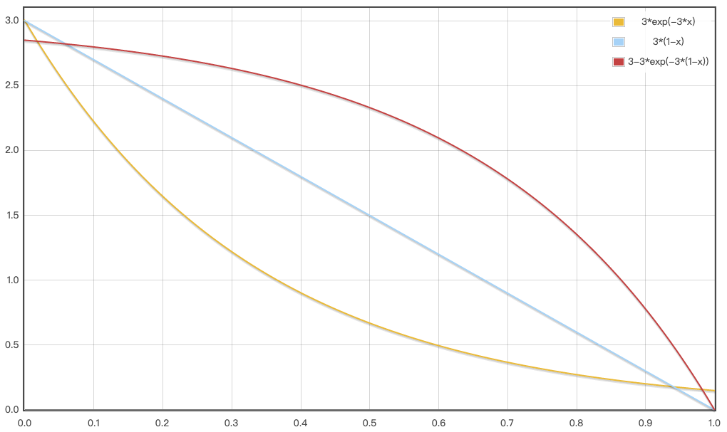
Figure 5: Visualization of the noise schedule of Noise decay A, Noise decay B and Noise decay C.

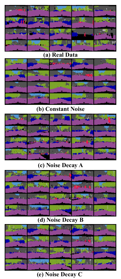
Figure 6: Additional samples from real data, Constant Noise, Noise decay A, Noise decay B and Noise decay C.

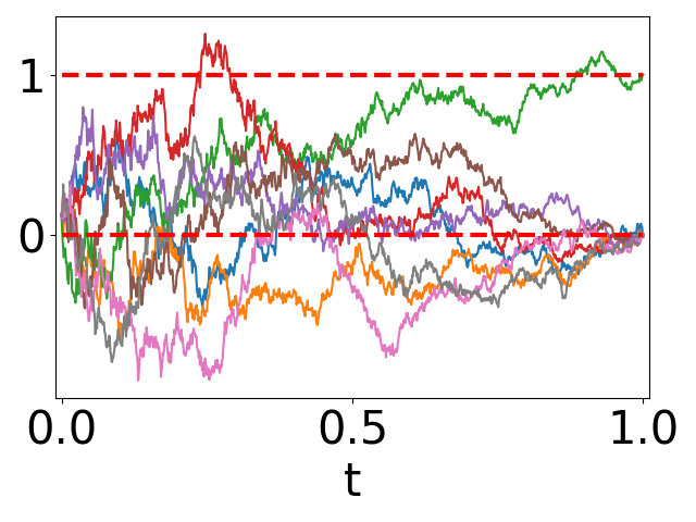
Figure 7: Diffusion process of one pixel (a $8$-dimensional vector) in CityScapes. As $t\rightarrow 1$, 7 of the dimensions reaches $0$, while 1 of the dimensions reaches $1$, turning the vector into a one-hot vector.

B.3 Continuous CIFAR10 generation

We provide additional results on generating CIFAR10 images in the continuous domain. The model is trained using the same training strategy as DDPM (Ho et al., 2020) with the code base provided in (Song et al., 2020b). Specifically, the neural network is the same U-Net structure as the implementation in (Song et al., 2020b). The optimizer is Adam with a learning rate of $0.0002$. According to common practice (Song and Ermon, 2020; Song et al., 2020b), the training is smoothed by exponential moving average (EMA) with a factor of $0.999$. The results are shown in Figure 8 and Table 5. We use $K=1000$ and $\mathrm{d}t=0.001$ for discretizing the SDE. Bridge variants yields similar generation quality as other diffusion models.

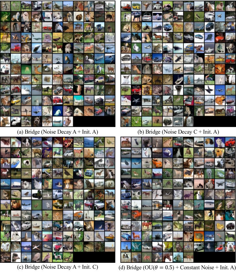
Figure 8: Samples for continuous CIFAR10 generation. Bridge variants can generate high-quality images.

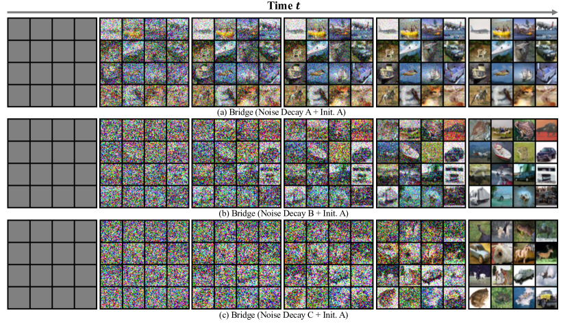
Figure 9: Sampling trajectory for continuous CIFAR10 generation with Noise Decay A, Noise Decay B, Noise Decay C. Bridge can generate images with different noise schedules.

B.4 Discrete CIFAR10 generation

The experiment details are similar to the continuous CIFAR10 generation, except that the domain of generation is limited to integer values. To account for the discretization error, after the final step, we apply rounding to the generated images to get real integer-valued images. We compare the value distribution of the generated images in Figure 10.

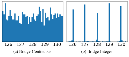
Figure 10: Final value distribution of the generated images with Bridge-Continuous and Bridge-Integer (before rounding) on CIFAR10. We only show the values in $[125.5,130.5]$ for visual clarity. Our Bridge-Integer generates discrete values.

Methods	IS	FID
Conditional
EBM (Du and Mordatch, 2019)	8.30	37.9
JEM (Grathwohl et al., 2019)	8.76	38.4
BigGAN (Brock et al., 2018)	9.22	14.73
StyleGAN2+ADA (Karras et al., 2020)	10.06	2.67
Unconditional
NCSN (Song and Ermon, 2019)	8.87	25.32
NCSNv2 (Song and Ermon, 2020)	8.40	10.87
DDPM ($L$) (Ho et al., 2020)	7.67	13.51
DDPM ($L_{simple}$) (Ho et al., 2020)	9.46	3.17
Schrödinger (Wang et al., 2021)	8.14	12.32
Bridge (Constant Noise + Init. A)	8.22	9.80
Bridge (Noise Decay A + Init. A)	8.83	6.76
Bridge (Noise Decay B + Init. A)	8.84	6.52
Bridge (Noise Decay C + Init. A)	8.62	7.62
Bridge (Noise Decay A + Init. B )	8.82	7.21
Bridge (Noise Decay A + Init. C )	8.75	6.28
Bridge (OU($\theta=0.1$) + Constant Noise + Init. A)	8.15	10.94
Bridge (OU($\theta=0.5$) + Constant Noise + Init. A)	8.19	10.85

Table 5: Additional results on continuous CIFAR10 generation. ‘Init.’ refers to ‘Initialization’. Bridge yields comparable IS and FID with other diffusion models.

Appendix C Broader Impact

This paper focuses on theoretical analysis of diffusion models. In terms of social impact, our method aims to open the black-box of diffusion generative models, and hence increase the interpretability and reliability of this family of ML models. Yet, it is not impossible to use the generative models for the generation of harmful contents. We believe how to incorporate the safety constraints into the generative models is still a valuable open question.

References

- Anderson (1982) Brian DO Anderson. Reverse-time diffusion equation models. Stochastic Processes and their Applications, 12(3):313–326, 1982.
- Austin et al. (2021) Jacob Austin, Daniel D Johnson, Jonathan Ho, Daniel Tarlow, and Rianne van den Berg. Structured denoising diffusion models in discrete state-spaces. Advances in Neural Information Processing Systems, 34:17981–17993, 2021.
- Bernardini et al. (1999) Fausto Bernardini, Joshua Mittleman, Holly Rushmeier, Cláudio Silva, and Gabriel Taubin. The ball-pivoting algorithm for surface reconstruction. IEEE transactions on visualization and computer graphics, 5(4):349–359, 1999.
- Brock et al. (2018) Andrew Brock, Jeff Donahue, and Karen Simonyan. Large scale gan training for high fidelity natural image synthesis. arXiv preprint arXiv:1809.11096, 2018.
- Burda et al. (2016) Yuri Burda, Roger B Grosse, and Ruslan Salakhutdinov. Importance weighted autoencoders. In ICLR (Poster), 2016.
- Chang et al. (2015) Angel X Chang, Thomas Funkhouser, Leonidas Guibas, Pat Hanrahan, Qixing Huang, Zimo Li, Silvio Savarese, Manolis Savva, Shuran Song, Hao Su, et al. Shapenet: An information-rich 3d model repository. arXiv preprint arXiv:1512.03012, 2015.
- Chen et al. (2020) Nanxin Chen, Yu Zhang, Heiga Zen, Ron J Weiss, Mohammad Norouzi, and William Chan. Wavegrad: Estimating gradients for waveform generation. In International Conference on Learning Representations, 2020.
- Cordts et al. (2016) Marius Cordts, Mohamed Omran, Sebastian Ramos, Timo Rehfeld, Markus Enzweiler, Rodrigo Benenson, Uwe Franke, Stefan Roth, and Bernt Schiele. The cityscapes dataset for semantic urban scene understanding. In Proc. of the IEEE Conference on Computer Vision and Pattern Recognition (CVPR), 2016.
- Dhariwal and Nichol (2021) Prafulla Dhariwal and Alexander Nichol. Diffusion models beat gans on image synthesis. Advances in Neural Information Processing Systems, 34, 2021.
- Doob and Doob (1984) Joseph L Doob and JI Doob. Classical potential theory and its probabilistic counterpart, volume 549. Springer, 1984.
- Du and Mordatch (2019) Yilun Du and Igor Mordatch. Implicit generation and modeling with energy based models. Advances in Neural Information Processing Systems, 32, 2019.
- Grathwohl et al. (2019) Will Grathwohl, Kuan-Chieh Wang, Jörn-Henrik Jacobsen, David Duvenaud, Mohammad Norouzi, and Kevin Swersky. Your classifier is secretly an energy based model and you should treat it like one. arXiv preprint arXiv:1912.03263, 2019.
- Heusel et al. (2017) Martin Heusel, Hubert Ramsauer, Thomas Unterthiner, Bernhard Nessler, and Sepp Hochreiter. Gans trained by a two time-scale update rule converge to a local nash equilibrium. Advances in neural information processing systems, 30, 2017.
- Ho et al. (2019) Jonathan Ho, Xi Chen, Aravind Srinivas, Yan Duan, and Pieter Abbeel. Flow++: Improving flow-based generative models with variational dequantization and architecture design. In International Conference on Machine Learning, pages 2722–2730. PMLR, 2019.
- Ho et al. (2020) Jonathan Ho, Ajay Jain, and Pieter Abbeel. Denoising diffusion probabilistic models. Advances in Neural Information Processing Systems, 33:6840–6851, 2020.
- Ho et al. (2022) Jonathan Ho, Chitwan Saharia, William Chan, David J Fleet, Mohammad Norouzi, and Tim Salimans. Cascaded diffusion models for high fidelity image generation. Journal of Machine Learning Research, 23(47):1–33, 2022.
- Hoogeboom et al. (2021) Emiel Hoogeboom, Didrik Nielsen, Priyank Jaini, Patrick Forré, and Max Welling. Argmax flows and multinomial diffusion: Learning categorical distributions. Advances in Neural Information Processing Systems, 34, 2021.
- Huang et al. (2021) Chin-Wei Huang, Jae Hyun Lim, and Aaron C Courville. A variational perspective on diffusion-based generative models and score matching. Advances in Neural Information Processing Systems, 34:22863–22876, 2021.
- Karras et al. (2020) Tero Karras, Miika Aittala, Janne Hellsten, Samuli Laine, Jaakko Lehtinen, and Timo Aila. Training generative adversarial networks with limited data. Advances in Neural Information Processing Systems, 33:12104–12114, 2020.
- Kong and Ping (2021) Zhifeng Kong and Wei Ping. On fast sampling of diffusion probabilistic models. In ICML Workshop on Invertible Neural Networks, Normalizing Flows, and Explicit Likelihood Models, 2021.
- Kong et al. (2020) Zhifeng Kong, Wei Ping, Jiaji Huang, Kexin Zhao, and Bryan Catanzaro. Diffwave: A versatile diffusion model for audio synthesis. In International Conference on Learning Representations, 2020.
- Lejay (2018) Antoine Lejay. The girsanov theorem without (so much) stochastic analysis. In Séminaire de Probabilités XLIX, pages 329–361. Springer, 2018.
- Léonard et al. (2014) Christian Léonard, Sylvie Rœlly, and Jean-Claude Zambrini. Reciprocal processes. a measure-theoretical point of view. Probability Surveys, 11:237–269, 2014.
- Liu et al. (2021) Xingchao Liu, Xin Tong, and Qiang Liu. Sampling with trusthworthy constraints: A variational gradient framework. Advances in Neural Information Processing Systems, 34:23557–23568, 2021.
- Luo and Hu (2021a) Shitong Luo and Wei Hu. Diffusion probabilistic models for 3d point cloud generation. In Proceedings of the IEEE/CVF Conference on Computer Vision and Pattern Recognition, pages 2837–2845, 2021a.
- Luo and Hu (2021b) Shitong Luo and Wei Hu. Score-based point cloud denoising. In Proceedings of the IEEE/CVF International Conference on Computer Vision, pages 4583–4592, 2021b.
- Nichol and Dhariwal (2021) Alexander Quinn Nichol and Prafulla Dhariwal. Improved denoising diffusion probabilistic models. In International Conference on Machine Learning, pages 8162–8171. PMLR, 2021.
- Oksendal (2013) Bernt Oksendal. Stochastic differential equations: an introduction with applications. Springer Science & Business Media, 2013.
- Peluchetti (2021) Stefano Peluchetti. Non-denoising forward-time diffusions. 2021.
- Ramesh et al. (2022) Aditya Ramesh, Prafulla Dhariwal, Alex Nichol, Casey Chu, and Mark Chen. Hierarchical text-conditional image generation with clip latents. arXiv preprint arXiv:2204.06125, 2022.
- Salimans et al. (2016) Tim Salimans, Ian Goodfellow, Wojciech Zaremba, Vicki Cheung, Alec Radford, and Xi Chen. Improved techniques for training gans. Advances in neural information processing systems, 29, 2016.
- Song et al. (2020a) Jiaming Song, Chenlin Meng, and Stefano Ermon. Denoising diffusion implicit models. In International Conference on Learning Representations, 2020a.
- Song and Ermon (2019) Yang Song and Stefano Ermon. Generative modeling by estimating gradients of the data distribution. Advances in Neural Information Processing Systems, 32, 2019.
- Song and Ermon (2020) Yang Song and Stefano Ermon. Improved techniques for training score-based generative models. Advances in neural information processing systems, 33:12438–12448, 2020.
- Song et al. (2020b) Yang Song, Jascha Sohl-Dickstein, Diederik P Kingma, Abhishek Kumar, Stefano Ermon, and Ben Poole. Score-based generative modeling through stochastic differential equations. In International Conference on Learning Representations, 2020b.
- Song et al. (2021) Yang Song, Conor Durkan, Iain Murray, and Stefano Ermon. Maximum likelihood training of score-based diffusion models. Advances in Neural Information Processing Systems, 34, 2021.
- Tzen and Raginsky (2019) Belinda Tzen and Maxim Raginsky. Theoretical guarantees for sampling and inference in generative models with latent diffusions. In Conference on Learning Theory, pages 3084–3114. PMLR, 2019.
- Uria et al. (2013) Benigno Uria, Iain Murray, and Hugo Larochelle. Rnade: The real-valued neural autoregressive density-estimator. Advances in Neural Information Processing Systems, 26, 2013.
- Van der Vaart (2000) Aad W Van der Vaart. Asymptotic statistics, volume 3. Cambridge university press, 2000.
- Vincent (2011) Pascal Vincent. A connection between score matching and denoising autoencoders. Neural computation, 23(7):1661–1674, 2011.
- Wang et al. (2021) Gefei Wang, Yuling Jiao, Qian Xu, Yang Wang, and Can Yang. Deep generative learning via schrödinger bridge. In International Conference on Machine Learning, pages 10794–10804. PMLR, 2021.
- Xiao et al. (2021) Zhisheng Xiao, Karsten Kreis, and Arash Vahdat. Tackling the generative learning trilemma with denoising diffusion gans. arXiv preprint arXiv:2112.07804, 2021.
- Zhou et al. (2021) Linqi Zhou, Yilun Du, and Jiajun Wu. 3d shape generation and completion through point-voxel diffusion. In Proceedings of the IEEE/CVF International Conference on Computer Vision, pages 5826–5835, 2021.