Addition of tabulated equation of state and neutrino leakage support to IllinoisGRMHD
Ariadna Murguia-Berthier
Abstract
We have added support for realistic, microphysical, finite-temperature equations of state (EOS) and neutrino physics via a leakage scheme to IllinoisGRMHD, an open-source GRMHD code for dynamical spacetimes in the Einstein Toolkit. These new features are provided by two new, NRPy+-based codes: NRPyEOS, which performs highly efficient EOS table lookups and interpolations, and NRPyLeakage, which implements a new, AMR-capable neutrino leakage scheme in the Einstein Toolkit. We have performed a series of strenuous validation tests that demonstrate the robustness of these new codes, particularly on the Cartesian AMR grids provided by Carpet. Furthermore, we show results from fully dynamical GRMHD simulations of single unmagnetized neutron stars, and magnetized binary neutron star mergers. This new version of IllinoisGRMHD, as well as NRPyEOS and NRPyLeakage, is pedagogically documented in Jupyter notebooks and fully open source. The codes will be proposed for inclusion in an upcoming version of the Einstein Toolkit.
I Introduction
Magnetized fluid flows in dynamical spacetimes are a key driver of multimessenger phenomena, a prominent example of which was the gravitational-wave signal GW170817 Abbott et al. (2017a) and the coincident short gamma-ray burst GRB170817A Abbott et al. (2017b), originating from a binary system of two merging neutron stars (NSs). Self-consistent simulations of these systems require software capable of modeling the diverse physics of the problem, from relativistic general relativistic magnetohydrodynamics (GRMHD) fluid flows, to the hot degenerate matter described by a microphysical, finite-temperature equation of state (EOS), to the changes in matter composition and energy due to the emission and absorption of neutrinos and photons, to the rapidly changing spacetime dynamics involved in the merger and black hole (BH) formation.
Given the high demand for accurate simulations of these systems, it is unsurprising that multiple groups have developed their own codes, some of which specialize in GRMHD for stationary spacetimes, which can be used e.g., for studying merger remnants Gammie et al. (2003); Noble et al. (2006, 2009); Murguia-Berthier et al. (2021); Anderson et al. (2006); while others are intended to model more generic GRMHD flows in dynamical spacetimes, which can be used for inspiral, merger, and post-merger dynamics Bruegmann et al. (2008); O’Connor and Ott (2010); Thierfelder et al. (2011); Giacomazzo and Rezzolla (2007); Cerda-Duran et al. (2008); Kiuchi et al. (2012); Dionysopoulou et al. (2013); Radice and Rezzolla (2012); Radice et al. (2014a, b); Mösta et al. (2014); White et al. (2016); Etienne et al. (2015, 2020); Kidder et al. (2017); Fernando et al. (2019); Felker and Stone (2018); Most et al. (2019); Cipolletta et al. (2020, 2021); Stone et al. (2020); Mewes et al. (2020); Tichy et al. (2020). Having many codes means that a variety of algorithmic choices are made during their development, some of which impact performance, some the code’s suitability to model certain physical systems, and others the physical realism of the simulations.
Examples of differences that affect a code’s performance and/or its ability to accurately model certain physical systems include the numerical resolution and adopted coordinate system (e.g., Cartesian, spherical, etc.); how spatial derivatives are represented numerically (e.g., finite difference, finite volume, discontinuous Galerkin, spectral, or even hybrid methods); the choice of EOS; and how neutrino effects are modeled; just to name a few.
Regarding the EOS, a common choice made by many codes is a simple ideal gas EOS, accounting for temperature effects through a thermal contribution Janka et al. (1993). Others improve the description of the cold (as opposed to thermal) portion of the EOS by adopting the so-called piecewise polytropic model (see e.g., Read et al. (2009) and references therein). Finally, some codes adopt microphysical, finite-temperature EOS tables constructed using data from astrophysical observations and nuclear physics experiments, like the ones available in the CompOSE Typel et al. (2015); Oertel et al. (2017); Typel et al. (2022) and Stellar Collapse stellarcollapse website (2022) databases. These tables provide the best description of nuclear matter available to date.
Regarding neutrino effects, one may consider the general relativistic radiation magnetohydrodynamics (GRRMHD) equations and model neutrino transport via Monte Carlo methods—by far the most computationally expensive option. These methods try to solve the seven-dimensional Boltzmann’s equation by grouping particles into packets that approximate the distribution function of neutrinos at random points. We mention here in particular the works of Foucart et al. Foucart et al. (2020, 2021a, 2021b) and Miller et al. Miller et al. (2019a, b), which have used this technique in the context of binary neutron star (BNS) mergers. It is important to note that this method becomes prohibitively expensive in the optically thick regime (high densities and temperatures), requiring e.g., enforcing a hard ceiling on the value of the absorption opacity of the fluid Foucart et al. (2021a).
Another approximate method for modeling neutrino physics is moment-based radiation transport. In this technique, the Boltzmann equation is recast as a system Thorne (1981); Shibata et al. (2011), which is then solved using similar numerical techniques to those for the GRMHD equations. Unlike the GRMHD equations, however, the system cannot be closed with an EOS, making its accuracy dependent on the choice of closure (see e.g., Richers (2020)). This method has also been used in many studies, including core-collapse Obergaulinger et al. (2014); O’Connor (2015); Kuroda et al. (2016); O’Connor and Couch (2018); Roberts et al. (2016); Skinner et al. (2019); Glas et al. (2019); Rahman et al. (2019); Laiu et al. (2021) and BNS Foucart et al. (2015, 2016a, 2016b); Radice et al. (2022); Sun et al. (2022).
Leakage schemes are perhaps the most popular approach for modeling neutrino physics van Riper and Lattimer (1981); Ruffert et al. (1996); Rosswog and Ramirez-Ruiz (2002); Rosswog and Liebendoerfer (2003); Sekiguchi (2010); Sekiguchi et al. (2011). In this approach, experimental data are used to parameterize analytic formulas for the neutrino emission and cooling rates in terms of the optical depths, resulting in a computationally inexpensive algorithm that has been adopted rather broadly O’Connor and Ott (2010); Ott et al. (2012); Neilsen et al. (2014); Radice et al. (2016); Siegel and Metzger (2018); Endrizzi et al. (2020); Murguia-Berthier et al. (2021). It is important to state that leakage scheme typically neglect the absorption of neutrinos and therefore do not account for heating and lepton number changes due to neutrinos in the ejecta Just et al. (2021).
While these studies differ in how neutrinos are modeled, one aspect most share in common is that thHey were performed using software that is not freely available to everyone. Exceptions include the GRMHD codes GR1D O’Connor and Ott (2010); O’Connor (2015), WhiskyTHC Radice and Rezzolla (2012); Radice et al. (2014a, b), GRHydro Mösta et al. (2014), IllinoisGRMHD Etienne et al. (2015, 2020), SpeCTRE Kidder et al. (2017); Deppe et al. (2022), and Spritz Cipolletta et al. (2020, 2021); Giacomazzo et al. (2020); the neutrino leakage codes ZelmaniLeak O’Connor and Ott (2010); Ott et al. (2012) and THC_Leakage Radice et al. (2016); the moment-based radiation transport codes ZelmaniM1 Roberts et al. (2016) and M1Grey Kidder et al. (2017); Deppe et al. (2022); and the GRRMHD Monte Carlo code bhlight Miller et al. (2019a).
Here we introduce a major update to IllinoisGRMHD—a concise open-source rewrite of the Illinois numerical relativity group’s GRMHD code Duez et al. (2005) (henceforth OrigGRMHD), which exists within the Einstein Toolkit. This new version, which is also open-source Werneck and Etienne (2022), supports both finite-temperature, microphysical EOSs—via a new NRPy+ Ruchlin et al. (2018) module called NRPyEOS Werneck and Etienne (2022)—and neutrino physics via a leakage scheme—using the recently developed NRPy+-based code NRPyLeakage Werneck and Etienne (2022). This updated version will be proposed for inclusion in a future Einstein Toolkit release.
For well over a decade, both OrigGRMHD and IllinoisGRMHD have been used to model a plethora of astrophysical scenarios, including magnetized binary neutron stars (BNS) Liu et al. (2008); Paschalidis et al. (2012); Ruiz and Shapiro (2017); Tsokaros et al. (2019); Raithel et al. (2021); Sun et al. (2022); Armengol et al. (2021), binary BH-NS Etienne et al. (2008, 2009, 2012a, 2012b); Paschalidis et al. (2015); Ruiz et al. (2018, 2020a), BH accretion disks Farris et al. (2011, 2012); Gold et al. (2014a, b); Khan et al. (2018); Porth et al. (2019); Wessel et al. (2021), binary white dwarf-NS Paschalidis et al. (2011a, b), rotating NSs Etienne et al. (2006); Espino et al. (2019), gravitational collapse of supermassive stars Sun et al. (2017), magnetized Bondi accretion Etienne et al. (2010), and magnetized hypermassive neutron stars (HMNS) Duez et al. (2006a, b); Liu et al. (2007); Shibata et al. (2006a, b); Stephens et al. (2007); Ruiz et al. (2020b), to name a few. We also highlight Frankfurt/IllinoisGRMHD Most et al. (2019), whose feature set exceeds that of the original IllinoisGRMHD, but like OrigGRMHD is currently a closed-source code.
In contrast to these codes, IllinoisGRMHD is open source and part of the Einstein Toolkit Loffler et al. (2012), and in this work we introduce Einstein Toolkit thorns (or modules) for NRPyEOS and NRPyLeakage, named NRPyEOSET and NRPyLeakageET, respectively.111We will refer to these as simply NRPyEOS and NRPyLeakage unless discussing thorn-exclusive features. This new version of IllinoisGRMHD, along with NRPyEOS and NRPyLeakage, will be proposed for inclusion in a future release of the Einstein Toolkit, but in the meantime all codes are freely available for download at Werneck and Etienne (2022).
This paper is organized as follows. Sec. II provides an overview of the mathematical formulation of the GRMHD equations and of the neutrino leakage scheme. Sec. III describes the numerical methods and technical aspects of our codes. Sec. IV contains a series of challenging validation tests of the code, as well as results from simulations of single NSs, and magnetized, equal-mass BNS systems, with eventual BH formation. Sec. V contains closing remarks and plans for future work.
II Basic equations
Throughout the paper Greek letters are used to denote spacetime indices (range 0–3) and lowercase Roman letters to denote spatial indices (range 1–3), assuming Einstein summation convention. Unless stated otherwise, geometrized units are adopted, additionally assuming that . Temperatures are measured in .
The spacetime evolution is governed by Einstein’s equations,
| (1) |
where is the Einstein tensor and is the total stress-energy tensor. As written, these equations are not in a form immediately suitable for numerical integration. One such form is the initial value formulation built upon first splitting into the Arnowitt–Deser–Misner (ADM) form Arnowitt et al. (1962)
| (2) |
where , , and are the lapse function, the shift vector, and the metric, all defined on spatial hypersurfaces of constant coordinate time . With this decomposition Einstein’s equations can be split into sets of hyperbolic (time-evolution) and elliptic (constraints) PDEs, similar to Maxwell’s equations in differential form (see e.g., Baumgarte and Shapiro (2010) for a pedagogical review). The resulting ADM evolution and constraint equations are in fact not numerically stable, and must be reformulated further. The Baumgarte–Shapiro–Shibata–Nakamura (BSSN) formulation Nakamura et al. (1987); Shibata and Nakamura (1995); Baumgarte and Shapiro (1999) is one such reformulation in which additional auxiliary and conformal variables are introduced in order to make the resulting set of equations strongly hyperbolic, enabling stable, long-term time integration of Einstein’s equations on the computer.
The remainder of this section is dedicated to the GRMHD formulation used by IllinoisGRMHD, as well as an overview of the neutrino leakage scheme adopted by NRPyLeakage.
II.1 General relativistic magnetohydrodynamics
The GRMHD equations with neutrino leakage can be written as
| (3) | ||||
| (4) | ||||
| (5) | ||||
| (6) |
which are the conservation of baryon number, conservation of lepton number, conservation of energy-momentum, and homogeneous Maxwell’s equations, respectively. In the above, () is the baryon (lepton) number density, is the fluid four-velocity, is the baryon mass, is the dual of the Faraday tensor , and is the Levi-Civita tensor. Ideal MHD () is assumed throughout. The source terms and account for changes in lepton number and energy, respectively, due to the emission and absorption of neutrinos. The precise form of and is detailed in the next section on neutrino leakage.
The energy-momentum tensor is assumed to be that of a perfect fluid, plus an electromagnetic contribution, given by
| (7) |
where is the baryon density, is the specific enthalpy, is the specific internal energy, is the fluid pressure, is the rescaled 4-magnetic field in the fluid frame, where
| (8) | ||||
| (9) |
and is the magnetic field in the frame normal to the hypersurface.
To source Einstein’s equations must be updated from one time step to the next, which requires evolving the matter fields in time. To accomplish this, Eqs. (3)–(6) are rewritten in conservative form:
| (10) |
where and are the flux and source vectors, respectively. Furthermore, is the vector of conservative variables, with the vector of primitive variables. IllinoisGRMHD adopts the Valencia formalism Anton et al. (2006); Banyuls et al. (1997), whereby
| (11) |
Here, is the electron fraction, is the temperature, and is the fluid three-velocity. Notice that this choice of primitive three-velocity differs from the Valencia three-velocity used in other codes (see e.g., Baiotti et al. (2003, 2003); Giacomazzo and Rezzolla (2007); Mösta et al. (2014); Cipolletta et al. (2020, 2021)); IllinoisGRMHD adopts the 3-velocity that appears in the induction equation Eq. (14). These two velocities are related via
| (12) |
The conservative variables can be written in terms of the primitive variables as
| (13) |
where and is the Lorentz factor.
There are many numerical advantages associated with writing the GRMHD equations in conservative form. First, ignoring neutrino effects, the source terms vanish in flat space with Cartesian coordinates and this form of the equations, when combined with an appropriate finite-volume scheme, guarantees conservation of total rest mass, lepton number, energy, and momentum to roundoff error. Second, conservation is guaranteed up to errors in when the sources are nonzero. Third, IllinoisGRMHD adopts finite-volume methods, which are superior at handling ultrarelativistic flows as compared to easier-to-implement and more-efficient artificial viscosity schemes Marti et al. (1991); Anninos and Fragile (2003). Fourth, this conservative formulation enables us to easily use a high-resolution shock-capturing (HRSC) scheme, designed to minimize Gibbs’ oscillations near shocks, to name a few advantages.
An important consideration when implementing a GRMHD code is how to handle the magnetic induction equation, obtained from the spatial components of Eq. (6). In conservative form, this equation may be written as
| (14) |
If Eq. (14) were to be propagated forward in time, evaluating its spatial partial derivatives without special techniques, violations of the “no magnetic monopoles” condition (which follows from the time component of Eq. 6)
| (15) |
will grow with each iteration. Ensuring this constraint remains satisfied, particularly on AMR grids, is a nontrivial endeavor. We adopt the same strategy as the one used in Etienne et al. (2010, 2012c), which is to evolve the electromagnetic (EM) four-potential instead of the magnetic fields directly. In this case, numerical errors associated with evolving do not impact violations of Eq. (15), as the magnetic field is computed as the “curl” (i.e., a Newtonian curl with definition appropriately generalized for GR) of the vector potential, and the divergence of the curl is by definition zero (here to roundoff error, once a numerical approximation for partial derivative is chosen).
The decomposition of the vector potential gives (see e.g., Baumgarte and Shapiro (2021) for a pedagogical review)
| (16) |
where is the unit vector normal to the spatial hypersurface, is the purely spatial (i.e., ) magnetic potential, is the electric potential, and is the totally antisymmetric Levi-Civita symbol, with . Thus Eq. (14) becomes
| (17) |
We fix the EM gauge by adopting a covariant version of the “generalized Lorenz gauge condition”,
| (18) |
which was first introduced by the Illinois relativity group in Etienne et al. (2012c); Farris et al. (2012). Here is a parameter with units of inverse length, chosen so that the Courant–Friedrichs–Lewy (CFL) condition is always satisfied. Typically is set to , where is the time step of the coarsest refinement level (see Mewes et al. (2020) for further details). This gauge condition results in the additional evolution equation
| (19) |
where .
Except for Eqs. (17) and (19), the remaining GRMHD equations are evolved using Eq. (10) and a HRSC scheme, as described in Etienne et al. (2015). For completeness, the remaining components of the flux vector are given by
| (20) |
and those of the source vector are given by
| (21) |
where
| (22) |
and is the extrinsic curvature.
Specifying the matter EOS closes this system of equations. To this end, IllinoisGRMHD supports both analytic, hybrid EOSs Janka et al. (1993) as well as microphysical, finite-temperature, fully tabulated EOSs.
For tabulated EOSs, hydrodynamic quantities are given as functions of the density , the electron fraction , and the temperature . As needed, the temperature can be recovered from the pressure, specific internal energy, or entropy by using either a Newton–Raphson method or bisection, with the latter yielding superior results in highly degenerate regions of parameter space.
These table operations are handled by NRPyEOS, a pedagogically documented and infrastructure-agnostic NRPy+ module that generates table interpolation routines based on the Einstein Toolkit’s core EOS driver thorn EOS_Omni, which is itself based on the original code by O’Connor & Ott O’Connor and Ott (2022). NRPyEOS provides a clean and clear user interface, generating specialized routines that compute only needed hydrodynamic quantities, avoiding unnecessary interpolations and thus greatly increasing the overall performance of GRMHD simulations that make use of tabulated EOSs.
A concrete example is the computation of the neutrino opacities and emission and cooling rates, for which NRPyLeakage requires five table quantities: , which are the chemical potentials of the electron, neutron, and proton, and the neutron and proton mass fractions, respectively. The general-purpose routine EOS_Omni_full is the only one available in EOS_Omni to compute such quantities. This routine, however, interpolates a total of 17 table quantities, 11 of which are unused for our purposes, resulting in it being twice as slow as the specialized routine generated by NRPyEOS.
For hybrid EOSs, hydrodynamic quantities are analytic functions of the density and the specific internal energy. The pressure is given by
| (23) |
where
| (24) |
accounts for thermal effects, with a constant parameter that determines the conversion efficiency of kinetic to thermal energy at shocks, and and are computed assuming either a gamma-law or piecewise polytropic EOS (see e.g., Read et al. (2009)).
II.2 Neutrino leakage
NRPyLeakage—a new infrastructure-agnostic neutrino leakage code generated by NRPy+ and fully documented in pedagogical Jupyter notebooks—enables us to incorporate basic neutrino physics in our simulations. Our implementation follows the prescription of Ruffert et al. (1996); Galeazzi et al. (2013); Siegel and Metzger (2018) to compute the neutrino number and energy emission rates, as well as the neutrino opacities. We also consider nucleon-nucleon Bremsstrahlung Burrows et al. (2006) following the ZelmaniLeak code O’Connor and Ott (2010); Ott et al. (2012); O’Connor and Ott (2011). Unlike Ruffert et al. (1996) and ZelmaniLeak, however, we adopt a local, iterative algorithm in order to compute the neutrino optical depths following Neilsen et al. (2014); Siegel and Metzger (2018) (see also Murguia-Berthier et al. (2021)) , yielding far more efficient computations of optical depths than that implemented in ZelmaniLeak when the modeled system is far from spherical symmetry. Further, the Einstein Toolkit version of the code has been carefully designed to work seamlessly with the Cartesian AMR grids provided by Carpet Schnetter et al. (2004).
Neutrinos are accounted for via the following reactions: -processes, i.e., electrons () being captured by protons () and positrons () being captured by neutrons (),
| (25) | ||||
| (26) |
electron-positron pair annihilation,
| (27) |
transverse plasmon () decay,
| (28) |
and nucleon-nucleon Bremsstrahlung,
| (29) |
In the reactions above are the electron, muon, and tau neutrinos, with their antineutrinos, and heavy nuclei. Our implementation assumes that the contributions from heavy lepton neutrinos and antineutrinos are all the same, and we use the notation to refer to any one species throughout.
The production of neutrinos via these processes lead to changes in the electron fraction and energy of the system, which are accounted for in the source terms and of Eqs. (4) and (5). More specifically,
| (30) | ||||
| (31) |
where the effective rates are given by
| (32) | ||||
| (33) |
and the diffusion time scales using
| (34) |
where are the neutrino optical depths, the total neutrino transport opacity (see Sec. III.2), Rosswog and Liebendoerfer (2003); O’Connor and Ott (2010); Siegel and Metzger (2018); Murguia-Berthier et al. (2021), and . The free emission time scales are given by
| (35) |
where and are the neutrino number and energy density, respectively, and the total free emission and cooling rates are given by
| (36) | ||||
| (37) |
Note that -processes only contribute when .
For small densities and temperatures—the optically thin regime—the optical depths vanish and the medium is essentially transparent to neutrinos. Diffusion occurs on much shorter time scales than free-streaming, and therefore the effective rates become the free ones. For large densities and temperatures—the optically thick regime—optical depths are large and the neutrinos interact with the matter, such that diffusion happens on long time scales and free-streaming on short ones due to the increase in the emission and cooling rates, implying and . The leakage scheme provides a smooth interpolation between the diffusive and free-streaming regimes (see Ruffert et al. (1996) for details). We postpone the discussion on how the optical depths are computed in NRPyLeakage until Sec. III.2.
III Numerical methods
Most of the core numerical algorithms in IllinoisGRMHD remain the same as in the original version announced in 2015; these algorithms were reimplemented from OrigGRMHD as they were found most robust when modeling a large variety of astrophysical scenarios. Core algorithms, as described in Etienne et al. (2015), include the HRSC scheme, the Harten–Lax–van Leer approximate Riemann solver Harten et al. (1983), the piecewise parabolic method Colella and Woodward (1984) used to reconstruct the primitive variables at the cell interfaces, the staggering of the electric and magnetic potentials and of the magnetic field, the algorithm to compute the magnetic fields from the magnetic potential, the Runge–Kutta time integration, and outflow boundary conditions.
Key algorithmic changes introduced here include an updated conservative-to-primitive infrastructure, which has been expanded to include new effective 1D routines that are well-suited for tabulated EOSs, and the interface with the newly developed codes NRPyEOS and NRPyLeakage. We reserve the remainder of this section to discussing these updates in detail.
III.1 Conservative-to-primitive recovery
The energy-momentum tensor in the GR field equations and the GRMHD equations are written as functions of the primitive variables. So after updating the conservative variables at each time iteration, the primitive variables (“primitives”) must be computed from the conservative variables (“conservatives”). This is a nontrivial step, as there are no algebraic expressions to compute the conservatives from the primitives, requiring the implementation of a root-finding algorithm to solve a set of coupled nonlinear equations.
As numerical errors—such as truncation error originating from spatial and temporal finite differencing, as well as interpolation and prolongation operations—can cause the conservative variables to stray away from their valid range, sometimes this inversion becomes impossible. Because of this, we perform a series of checks on conservative variables to ensure they are valid before attempting to recover the primitive variables. We refer the reader to Appendix A of Etienne et al. (2012a) for details on how these bounds are checked and enforced.
For gamma-law and hybrid EOSs, the primary primitive recovery routine used in IllinoisGRMHD is the 2D scheme of Noble et al. Noble et al. (2006) (henceforth “Noble 2D”).222The dimensionality of the scheme is associated with how many equations are used to recover the primitive variables: 1D schemes use one equation and one unknown, 2D schemes use two equations and two unknowns, etc. We have also implemented the 1D scheme of the same reference, as well as 1D routines that replace the energy by the entropy, which is passively advected alongside the other variables assuming a conservation equation, as in Noble et al. (2009). The user is then given the option to use one or more of these last three routines as backups to the Noble 2D one.
The entropy routines perform well in regions of high magnetization and low densities, where the other two can be less robust, but we stress that they should only be used as backups, as the entropy is not conserved at shocks and therefore cannot always be reliably used to recover the primitives. If the Noble 2D and backup routines are unable to recover the primitives, a final backup routine due to Font et al. Font et al. (2000) is used, for which the pressure is reset to its cold value and thus an inversion is guaranteed (see Appendix A of Etienne et al. (2012a) for more details).
For tabulated EOSs, Newton–Raphson-based routines become very sensitive to the initial guesses provided for the primitive values. IllinoisGRMHD does not keep track of the values of the primitives at the previous time step, making it difficult to use routines such as the Noble 2D and the closely related routines by Antón et al. Anton et al. (2006), Giacomazzo & Rezzolla Giacomazzo and Rezzolla (2007), and Cerdá-Durán et al. Cerda-Duran et al. (2008) (see also Murguia-Berthier et al. (2021)).
As reviewed in Siegel et al. (2018), some routines require better initial guesses than others. In particular, we find that the 1D routines of Neilsen et al. Neilsen et al. (2014) and Palenzuela et al. Palenzuela et al. (2015), as well as the one by Newman & Hamlin Newman and Hamlin (2014), which only require an initial guess for the temperature, are very robust at recovering primitive variables even for relatively poor initial guesses. Our implementation of these routines is based on the open-source infrastructure by Siegel Siegel (2022), and we extend the implementation by adding to the routines the option of using the entropy instead of the energy during primitive recovery.
Performing an EOS table inversion with the entropy yields far smaller temperature errors than when using the energy—particularly in regions of high densities and low temperatures—and therefore, unsurprisingly, the modified routines recover the primitive variables with far smaller errors than the original. Unfortunately, because the entropy evolution assumes that entropy is conserved (an approximation that completely fails near shocks), these new routines are also only suitable as backup routines. As the entropy backup is rarely applied, and generally applied only far from shocks, we find it quite useful.
A primitive recovery step begins with guesses and or , corresponding to the atmospheric and maximum temperatures allowed in the simulation, which exist at or within the EOS table bounds. In this paper the values and are adopted. A density guess is obtained using and the electron fraction is recovered analytically from . All other primitives are computed from these using the EOS.
Both the Palenzuela et al. and Newman & Hamlin routines are iterative and result in updates to the Lorentz factor and specific internal energy (or entropy), requiring EOS table inversions to compute the temperature at every iteration. Starting with the energy version of the routines and , a primitive recovery is attempted using the Palenzuela et al. routine. A failure leads to a new attempt using the Newman & Hamlin routine. In case this fails, the temperature guess is reset to and the previous steps are repeated. If all previous steps fail, the process is repeated with the entropy version of the routines. If at the end of this step primitive recovery is still unsuccessful, the point is flagged and the recovery continues for the remaining grid points.
After sweeping the numerical grid once, we loop over flagged points, look at their neighbors and check for how many of them the primitive recovery has succeeded. If not enough neighbors are found the run is terminated, as clusters of failures indicate serious problems in the evolution. When the number of neighbors is sufficient, the conservative variables at the flagged points are set to
| (38) |
where denotes the average of the conservative variables at the neighboring points for which primitive recovery succeeded. This is repeated up to four times, successfully increasing the weight to , , , and in each new attempt. If primitive recovery is unsuccessful at this point, they are reset to their atmosphere values (, , and ).
We note that recovery failures are quite rare—particularly those in which all of the backup techniques fail—and typically occur in dynamically irrelevant regions: in the low density atmosphere or deep inside BH horizons. However, because production-quality simulations involve primitive recovery attempts, occasional failures are a near certainty. In the case of failures, adjusting the fluid 3-velocity components to zero is rather undesirable as it could greatly and discontinuously influence the magnetic field dynamics in regions that are magnetically dominated. With this in mind, we have dedicated considerable effort in making our backup strategies robust, avoiding velocity resets as much as possible.
Finally, we note that we have not extended the Font et al. routine to work with tabulated EOS, but this will be done in a future work. We also plan on using the tabulated EOS version of RePrimAnd Kastaun et al. (2021) once it becomes available.
III.2 Computation of optical depth
In NRPyLeakage we consider the following reactions contribute to the total transport opacities :
| (39) | |||||||||
| (40) | |||||||||
| (41) | |||||||||
| (42) |
The first two of these reactions are inverse -processes— absorption onto neutrons and absorption onto protons, respectively—and are the dominant contributions to the optical depths of and . The last two reactions describe neutral-current-scattering off neutrons, which provide the dominant contribution to the optical depths of heavy-lepton neutrinos. Explicit formulae for obtaining can be found in Appendix A of Ruffert et al. (1996).
Computing the local neutrino optical depths generally involves a global integration of along some path , i.e.,
| (43) |
One common option, implemented in the open-source code ZelmaniLeak, is to integrate along radial rays (see e.g., O’Connor and Ott (2010); Ott et al. (2012); O’Connor and Ott (2011)), which for simulations that use Cartesian coordinates require an auxiliary spherical grid. One interpolates data to the spherical grid, computes the opacities, and then performs the integration. This approach is particularly well-suited to study core collapse and other nearly spherically symmetric systems. However, for systems far from spherical symmetry, such as BNS and BH accretion disks, computing the optical depths this way can be very inefficient, as the resolution of the auxiliary spherical grids would need to be increased tremendously to produce accurate optical depths.
In order to have an algorithm that is both efficient and more generally applicable, we instead compute the optical depths with the local approach proposed in Neilsen et al. (2014) (see also Siegel and Metzger (2018); Murguia-Berthier et al. (2021)). The optical depths are first integrated to all of their nearest neighbors and then updated using the results that lead to the smallest optical depths, i.e.,
| (44) |
where is the grid spacing along the th-direction. For simplicity, we do not integrate diagonally. In this way neutrinos are allowed to explore many possible paths out of regions with relatively high optical thickness, following the path of least resistance. In our implementation, we assume that the outer boundary of the computational domain is transparent to neutrinos and thus have zero optical depths.
Because the opacities themselves depend on the optical depths, the following iterative approach is used to compute the initial optical depths at all gridpoints in the simulation domain. First the optical depths are initialized to zero, leading to an initial estimate of the opacities. This initial estimate is used to update the optical depths according to Eq. (44), which in turn allows us to recompute the opacities, and so on. One might also interpret this algorithm as considering only nearest neighbors in the first iteration, next-to-nearest neighbors in the second, next-to-next-to-nearest neighbors in the third, etc. In this way our algorithm enables neutrinos to map out paths of least resistance through arbitrary media.
When the grid structure contains multiple refinement levels, we adopt a multi-grid “V” cycle at each iteration: the optical depths are computed on a given refinement level and, unless we are at the finest one, the solution is prolongated to the next finer one; we move to the next finer refinement level and repeat the previous step; once the finest refinement level is reached the solution is restricted to the coarser levels, completing one iteration.
The algorithm is stopped once an equilibrium is reached, measured by the overall relative change in the optical depths between consecutive iterations ,
| (45) |
Once falls below a user-specified threshold (typically ) or the prescribed maximum allowed number of iterations (typically ) is exceeded, the algorithm stops.
IV Results
This section presents stress tests of these new algorithms implemented in IllinoisGRMHD, with the aim of demonstrating both the correctness of our implementation as well as its robustness when modeling challenging astrophysical scenarios.
To this end, we first present results from challenging unit tests of the conservative-to-primitive infrastructure and the optical depth framework. Further, to validate NRPyLeakage, we evolve a simple optically thin gas and compare results between IllinoisGRMHD and a trusted code with a physically identical but independently developed neutrino leakage scheme, HARM3D+NUC. Next to demonstrate the reliability of our new tabulated EOS implementation, NRPyEOS, we evolve isolated, unmagnetized NSs without neutrino leakage at different grid resolutions with different EOS tables. We consider the test as passed if numerically driven oscillations converge to zero with increased resolution at an order consistent with the reconstruction scheme (between second and third order for PPM).
The remaining tests focus on full-scale simulations of physical scenarios that lie at the heart of multimessenger astrophysics. We simulate magnetized, equal-mass BNS systems that lead to a remnant BH with an accretion disk that is evolved for several dynamical timescales. We perform simulations with and without our new neutrino leakage scheme, comparing the qualitative differences between them. Stably modeling these last two systems, in particular, is extremely difficult if the new algorithms are not implemented correctly, thus acting as the most strenuous tests conducted in our study.
In tests involving tabulated EOSs, we use three different fully-tabulated microphysical EOSs: the Lattimer–Swesty EOS with incompressibility modulus Lattimer and Swesty (1991) (henceforth LS220), the Steiner–Hempel–Fisher EOS Steiner et al. (2013) (henceforth SFHo), and the SLy4 EOS of Chabanat et al. (1998). For the first three, we use the tables by O’Connor–Ott O’Connor and Ott (2010), while for the last one we use the table by Schneider–Roberts–Ott Schneider et al. (2017), all of which are freely available at stellarcollapse website (2022). These choices of EOS were made largely to facilitate direct comparisons with HARM3D+NUC in the case of BH accretion disks.
Finally, we note that the EOS tables were cleaned with a simple script to change the reference mass used in the tables in such a way that the specific internal energy is never negative. We also clean up some of the table entries to avoid superluminal sound speeds. These are standard procedures when using EOS tables from stellarcollapse website (2022).
IV.1 Primitive variables recovery
In order to validate our implementation of primitive recovery routines described in Sec. III.1, we perform similar tests to the ones described in Siegel et al. (2018); Murguia-Berthier et al. (2021). First a set of primitive variables is specified and conservatives computed. Then the primitive recovery routine is selected and the conservatives injected into it. The primitives that are output from the recovery routine are compared with the input primitives, producing an estimate of how well the tested routine is able to recover the correct primitive variables. We refer to this as a “ to to ” test.
We measure the primitive recovery error at each recovery as a sum of relative errors across all primitive variables in the primitives vector
| (46) |
where and represent the original and recovered primitive variables, respectively, and the sum includes all variables in Eq. (11).
For a given EOS, we perform two separate tests in which we use points to evenly discretize non-constant hydrodynamic quantities. In the first test we consider , and arbitrarily fix the electron fraction to , the Lorentz factor to , and the magnetic pressure to ; in the second we consider , , and arbitrarily fix , , and . The pressure, specific internal energy, and entropy are computed using the EOS table, while the spatial components of the velocities and magnetic fields are set randomly from and , respectively. Finally, we compute the conservative variables using Eq. (13) assuming flat space.
We use this setup to test the Palenzuela et al. and the Newman & Hamlin routines as implemented in IllinoisGRMHD. As described in Sec. III.1, each routine is given two chances to recover the primitives, with initial guesses and, in case of failure, . In Fig. 1 we present the test results.
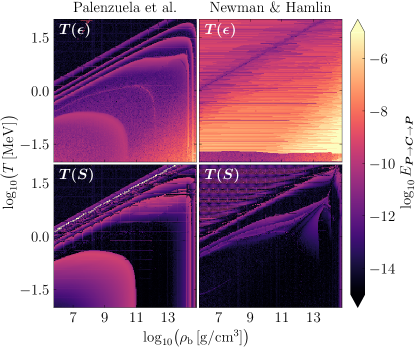
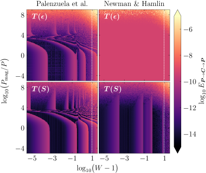
As our implementation allows for one to use either the specific internal energy or the entropy to recover the temperature, we perform tests using both. Our results indicate that using the entropy generally leads to errors that are at least comparable to, but often smaller than, those obtained using the energy. However, because IllinoisGRMHD currently adopts an approximate entropy evolution equation (assuming entropy is conserved), we are unable to reliably use the entropy as our default variable for primitive recovery. During actual numerical evolutions, we thus limit use of the entropy variable to a backup when recovery using the specific internal energy fails.
Further stress tests of the routines indicate they are robust for magnetizations as high as , although the recovery errors increase for . We also found that the routines typically fail to recover the primitives for , which is not worrisome given we impose a hard ceiling on the Lorentz factor which is much smaller than this value ( in the simulations presented in this paper).
IV.2 Optically thin gas
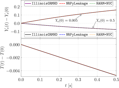
To validate our neutrino leakage implementation NRPyLeakage, we model an isotropic gas of constant density at rest in flat space assuming the SLy4 EOS. We note that this system has been chosen for its simplicity, not its physical relevance, as it allows us to validate the implementation of our leakage scheme against a trusted code.
In this scenario, the GRMHD equations simplify to
| (47) |
These equations are solved straightforwardly with a standalone code, which supports both NRPyLeakage and the leakage scheme of HARM3D+NUC. We then compare the results from these equations against those generated when IllinoisGRMHD evolves the full set of GRMHD equations. Agreement between IllinoisGRMHD and the standalone code provides an external validation of NRPyLeakage in the optically thin regime, as well as its integration within IllinoisGRMHD.
The solution has the following behavior. When the electron fraction is large (small), electron (positron) capture by protons (neutrons) is favored, resulting in a decrease (increase) of electron neutrinos (antineutrinos) and a decrease (increase) of the electron fraction with time. Note that, by construction, and thus the specific internal energy and temperature are always expected to decrease.
We perform two tests to verify the expected behavior of the system as described above. In one test we set the initial electron fraction to , while in the other we set it to . In both cases the density and initial temperature of the gas are set to and , respectively. Other hydrodynamic quantities, like the initial specific internal energy, are computed as needed using the SLy4 EOS of Schneider et al. (2017).
In Fig. 2 we show the excellent agreement between the results obtained by the different codes.333The leakage scheme in HARM3D+NUC assumes that the optical depths are always large when computing the neutrino degeneracy parameters. This is a reasonable assumption, given that most physical systems of interest are not transparent to neutrinos. Nevertheless, this causes a discrepancy between the leakage scheme in HARM3D+NUC and NRPyLeakage. For the sake of the comparison made here, we slightly modified the way HARM3D+NUC computes the neutrino degeneracy parameters to match what is done in NRPyLeakage; i.e., using Eqs. (A3) and (A4) in Ruffert et al. (1996).
IV.3 Optically thick sphere
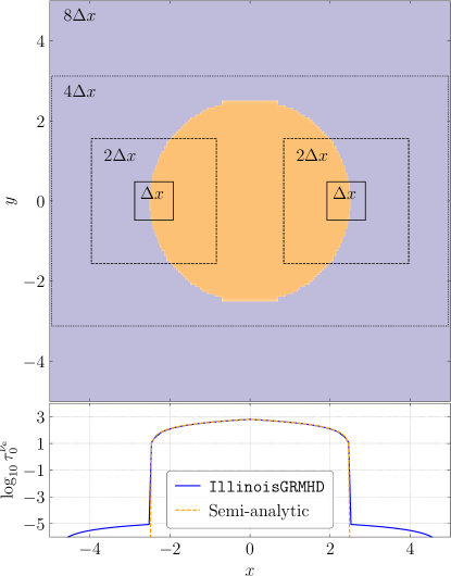
We next demonstrate the robustness of our implementation of the optical depth initialization algorithm on Cartesian AMR grids. To this end, a simple case of a sphere of constant density, electron fraction, and temperature is considered, for which the opacities vanish everywhere except in the interior of the sphere.
Given the opacities for this spherically symmetric system, the optical depths can also be determined semi-analytically by performing the integral Eq. (43) along radial rays, allowing us to validate our iterative algorithm. Since are constant, so are the opacities, yielding
| (48) |
The sphere is assumed to have radius , constant density , electron fracton , and temperature in an optically thin medium with , , and . We adopt the SLy4 EOS of Schneider et al. (2017).
Our grid is a Cartesian box of side-length with four refinement levels, as illustrated in the upper panel of Fig. 3. We add two refinement centers located at , each with three levels of refinement. Of course, this grid structure would never be used to simulate a spherical object, but because the surface of the sphere crosses multiple refinement boundaries, it provides a significantly challenging test for our optical depth initialization algorithm as detailed in Sec. III.2. We find excellent agreement with the semi-analytic results obtained using the opacities from the iterative algorithm in Eq. (48) , as shown in the bottom panel of the figure.
IV.4 Tolman–Oppenheimer–Volkoff star
As our next validation test, we evolve unmagnetized, stable Tolman–Oppenheimer–Volkoff (TOV) NSs. In this test, we disable neutrino leakage to ensure the NS maintains this equilibrium solution in the continuum limit. That is to say, in the limit of infinite numerical resolution, we expect zero oscillations in our simulated NSs.
When placing the stars in our finite resolution numerical grids however, numerical errors induce stellar oscillations. Because these oscillations are largely caused by truncation error associated with IllinoisGRMHD’s reconstruction scheme, they should converge to zero as we increase the resolution of the numerical grid. To confirm this, we perform simulations at three different resolutions—hereafter low (LR), medium (MR), and high (HR)—and demonstrate that the oscillations converge away at the expected rate.
To obtain initial data, a tabulated EOS is chosen and the TOV equations are solved using NRPy+’s TOV solver. Three different EOS tables are used: LS220, SFHo, and SLy4. The initial temperature is fixed to , while the initial electron fraction is determined by imposing the neutrino-free beta-equilibrium condition , where is the neutrino chemical potential. The initial data are then evolved forward in time with the Einstein Toolkit, using Baikal Etienne (2022) and IllinoisGRMHD to perform the spacetime and GRMHD evolutions, respectively.
The numerical grid structure contains five factor-of-two levels of Cartesian AMR, with resolutions on the finest level of . The stars are evolved for approximately dynamical timescales
| (49) |
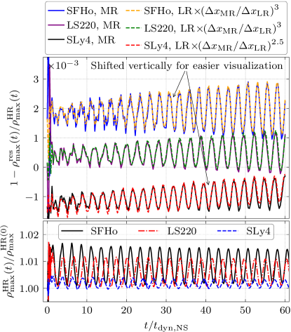
where is the maximum initial density (i.e., the density at the center of the NS). We monitor the maximum density on the grid as a function of time, with results from the HR runs displayed on the bottom panel of Fig. 4.
The top panel of Fig. 4 displays the relative errors, , of the oscillations from the MR and LR runs against the oscillations from the HR run. Assuming , we find
| (50) |
Thus, for a numerical scheme that is -order accurate, we expect that multiplying the relative errors of the LR run by will yield similar errors as the MR run. Generally we would expect the numerical errors to be dominated by our reconstruction method (PPM), which is between second and third order. This is indeed the observed behavior—the convergence order of our numerical scheme is found to be .
IV.5 Magnetized binary neutron stars
With the core new features validated, we now turn our attention to fully dynamical GRMHD simulations of a magnetized, equal-mass BNS system, modeling the inspiral, merger, and the resulting remnant BH. We adopt the LS220 microphysical, finite-temperature EOS, and simulate the system both with and without neutrino leakage enabled. This self-validation test is quite challenging, and is bound to result in unphysical behavior or, in the worst case, code crashes, if there are issues in our implementation.
Initial data are obtained using LORENE Gourgoulhon et al. (2001); Feo et al. (2017); Gourgoulhon et al. (2016, 2022). The initial separation of the system is and the gravitational (baryonic) mass of each NS is (), while the total ADM mass of the system is . The interior of each NS is seeded with a poloidal magnetic field with maximum initial value (see Appendix C of Etienne et al. (2015)). The initial temperature is set to and the electron fraction is determined by imposing the neutrino-free beta-equilibrium condition.
Baikal, which solves Einstein’s equations in the BSSN formalism, is used to evolve the spacetime. Again the Carpet AMR infrastructure is adopted to set up a grid with eight refinement levels by factors of two, with the resolution at the finest level . Upon BH formation, two additional refinement levels are added to better resolve the puncture, and thus the highest resolution on the grid becomes .
Performing the simulation using the Einstein Toolkit gives us access to outstanding diagnostic thorns, of which prominent examples include AHFinderDirect Thornburg (2004)—used to locate and compute the shape of apparent horizons—and QuasiLocalMeasures Dreyer et al. (2003); Schnetter et al. (2006)—used to compute useful quasi-local quantities like the BH mass and spin. Additionally, IllinoisGRMHD carefully monitors the number of times the primitive recovery infrastructure resorts to backup strategies, as well as the strategies used, aborting the simulation if any major error is detected. For the two simulations performed in this paper, we have not observed atmosphere resets or conservative averages (see Sec. III.1), which reflects the robustness of our conservative-to-primitive implementation.
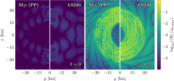
Satisfaction of the Einstein constraints reflect the health of BNS simulations in a holistic sense. As evidence that our updated implementation of IllinoisGRMHD is working correctly, we carefully monitor the Hamiltonian constraint violation throughout the numerical evolution. In Fig. 5 the magnitude of these violations with the LS220 tabulated EOS is compared against an evolution of an SLy piecewise polytropic EOS (PPEOS) BNS evolution performed with a trusted version of IllinoisGRMHD with hybrid equation of state support (adopting a PPEOS for the cold pressure). Both are equal-mass binaries (but run without any symmetries imposed), with each neutron star having a baryonic mass of and in the tabulated and PPEOS cases, respectively. The initial separations are different, so as to reuse existing data; this has no bearing on our assessment. The left panel of Fig. 5 displays side-by-side comparisons of this diagnostic at and, in the right panel, after a full orbit at .444Note that corresponds to different physical times in different simulations, but is unambiguously defined as the time it takes the stars to complete their first orbit. Initial violations are smaller for the PPEOS case, as the LORENE initial data possessed higher spectral resolution. The small initial constraint violation difference is quickly dominated by numerical-evolution errors, such that after one full orbit, constraint violations quickly reach a steady-state a few orders of magnitude higher than in the initial data. Generally we would expect that errors due to EOS table interpolations would result in slightly higher constraint violations in the tabulated EOS case, but we find that both runs exhibit quite comparable results.
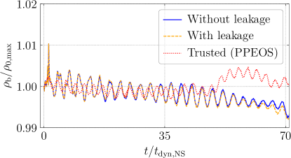
As in the TOV tests, we also track the maximum density on the grid over time—i.e., the density at the center of the NSs during inspiral. Fig. 6 shows the evolution of this quantity for 70 dynamical timescales, which happens to be shortly before merger in the tabulated EOS (LS220) case. As can be seen in the figure, the maximum density remains constant to 0.75% of its initial value throughout, indicating that the hydrostatic equilibrium of the NSs, imposed by the initial data, is maintained through merger, and to a degree that is comparable or better when comparing the latest IllinoisGRMHD against the trusted PPEOS version. Further, as expected, data in this figure demonstrate that neutrino leakage has no impact on the central densities of the neutron stars.
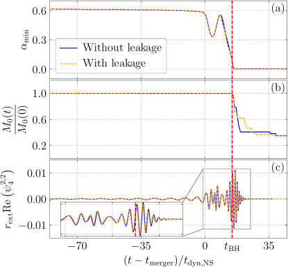
Next we focus on the merger of the tabulated EOS (LS220) BNS simulations, comparing results both with and without neutrino leakage enabled. BH formation occurs in coincidence with the collapse of the lapse function toward zero. When , we trigger Carpet to add additional refinement levels to our grid (as previously described) so that the moderately spinning black hole is sufficiently resolved.
Further, post-merger oscillations of are monitored as an indication of how close the merger remnant (a very short-lived HMNS in this case) is to BH formation. As can be seen in Fig. 7(a), our simulations lead to a HMNS that undergoes a single oscillation prior to collapse to a BH, with an apparent horizon detected after merger. Comparing with a couple other equal-mass results in the literature with similar initial NS masses adopting this EOS, we find that both result in a short-lived HMNS remnant that collapses to a BH between (Kastaun and Galeazzi (2015), with each NS having isolated ADM mass ) and (Bernuzzi et al. (2016), with each NS having isolated ADM mass ). However a clean, apples-to-apples comparison cannot be made, as simulations in these references did not include magnetic fields, chose different initial separations, and adopted different numerical resolutions/grids. Indeed, further work is sorely needed to cleanly validate current HMNS lifetime estimates across different codes, and we plan to perform such comparisons in future work.
As further validation that our conservative GRMHD scheme is working correctly, conservation of rest mass, i.e.,
| (51) |
is carefully monitored. Provided GRMHD flows do not cross AMR refinement levels or a black hole forms, this conservation should be maintained to roundoff error. Indeed, Fig. 7(b) demonstrates that the initial value is conserved to 0.001% throughout the inspiral for over 75 dynamical timescales. During and after BH formation, a significant amount of rest mass forms and falls into the horizon, where ceilings on maximum density are imposed for numerical stability and resulting in a loss of rest mass.
Finally, the gravitational wave signal, from the inspiralling of two NSs through the oscillations of the HMNS, to the ringing BH, is one of the key theoretical predictions derived from these simulations. In Fig. 7(c) we display the real component of the dominant, mode of extracted at . We note that in this panel of the figure we also subtract the time that it takes for the wave to propagate from the center of the grid to .
Minor differences in the signal are observed between simulations with and without neutrino leakage, which we attribute to the great increase in neutrino production after the massive shock—and consequent heating—that occurs when the NSs merge. As the neutrinos leak, they carry energy and deleptonize the system, which help explain the small differences in the gravitational wave signals.
| Neutrino leakage enabled | Neutrino leakage disabled |

| Neutrino leakage enabled | Neutrino leakage disabled |
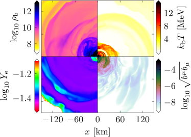
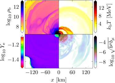
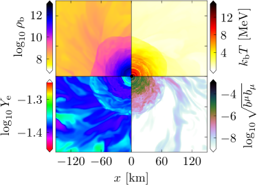
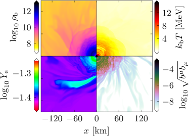
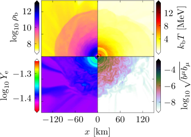
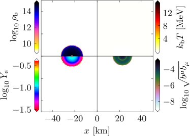
The gravitational wave signal already provides a hint that the inspiral phase of both simulations are virtually the same, and we confirm this behavior by looking at other quantities. In Fig. 8 snapshots of density, temperature, electron fraction, and are plotted on the orbital plane during the inspiral for the simulations with and without neutrino leakage. Indeed we observe no significant differences throughout.
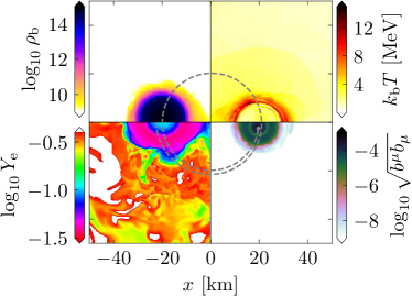
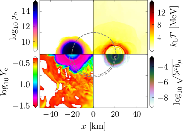
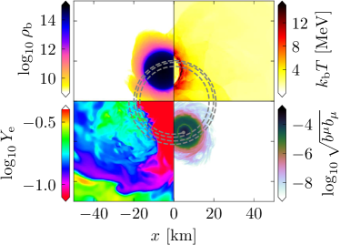
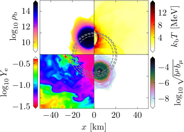
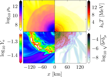
However, the post-merger phase of these simulations exhibit noticeable differences, as shown in Fig. 9. The BH accretion disk is slightly less neutron rich in the simulation with neutrino leakage enabled, with a large region of larger electron fraction being visible in the outer layers of the accretion disk. Notably, the same behavior is observed in HARM3D+NUC when studying magnetized BH accretion disks (see Fig. 11 of Murguia-Berthier et al. (2021)). A detailed analysis of the global quantities that characteriza the disk evolution (e.g., mass, radius, accretion rate, average , etc) will be the subject of a future work.
In this study we are only presenting results up to after black hole formation, when the spacetime already appears to be sufficiently static. We plan to use the recently developed HandOff code to transfer simulation data from IllinoisGRMHD to HARM3D+NUC and continue the post-merger phase for . Results of these continuation runs will be reported in a future publication.
V Conclusions & Future Work
Modeling magnetized compact binary systems in particular, and magnetized fluid flows in general, is of paramount importance for multimessenger astronomy. Simulating these systems accurately and reliably may not only lead to insights on phenomena we do not yet fully understand, but also provide crucial reference points for detections of gravitational waves and their electromagnetic and/or neutrino counterparts.
Given the importance of these simulations, many groups have developed GRMHD codes capable of performing them. Among these codes, the original GRMHD code developed by the Illinois numerical relativity group is particularly notable for its reliability and robustness when simulating a very broad range of astrophysical phenomena. Since IllinoisGRMHD acts as an open-source, drop-in replacement of the original code, it inherits all of the original code’s qualities while being faster and more concise.
The new version of IllinoisGRMHD presented in this work aims at improving not only technical aspects of the code, but also the physical realism of the simulations that it can perform. To this end, two key new features were added: support for microphysical, finite-temperature, tabulated EOSs via a new NRPy+-based code—NRPyEOS; and neutrino physics via a leakage scheme using another NRPy+-based code—NRPyLeakage.
IllinoisGRMHD has been developed to facilitate widespread community adoption. To this end, it was designed to be user-friendly, modular/extensible, robust, and performant/scalable. The development of this new version of the code shares all of these core principles, and it is with them in mind that we are making the code open-source and freely available for download Werneck and Etienne (2022).
In terms of user-friendliness, the code is well-documented, properly commented, and requires only basic programming skills to understand and run, traits also shared by NRPyEOS and NRPyLeakage. In the near future, we will release a series of Jupyter notebooks that meticulously document all of these codes.
Designed as thorns for the Einstein Toolkit and with clear separation of key algorithms in mind, all of these codes are both modular and extensible. To preserve the robustness of IllinoisGRMHD, every new addition has been rigorously tested to ensure maximum reliability and optimal performance. A systematic study of the scalability of the new version of IllinoisGRMHD, however, is not a focus of this work, in part because the core AMR infrastructure in the Einstein Toolkit is undergoing a major upgrade that will greatly improve scalability. IllinoisGRMHD will be made compatible with this updated infrastructure in the coming months.
It is widely known that moving from a simple, analytic EOS to a tabulated EOS and adding a neutrino leakage scheme negatively affects the code’s overall performance. In the case of IllinoisGRMHD, the new version of the code is about slower than the hybrid equation of state version. This performance impact is comparable to those observed by the authors of other codes, such as Spritz. A code comparison study that showcases the performance and impact of different algorithmic choices made by different GRMHD codes will be the subject of future work.
The BNS results presented in this paper exist as a part of a larger project. Because of this, we have taken special care to ensure that all of the new features in IllinoisGRMHD are consistent with those in HARM3D+NUC Murguia-Berthier et al. (2021). The simulation data will be transferred from IllinoisGRMHD to HARM3D+NUC (a code specially designed to accurately and reliably model BH accretion disks) using our recently developed HandOff code Armengol et al. (2021), and the simulation will continue for . Results of these simulations will be presented in a future paper.
Acknowledgments
The authors would like to thank E. O’Connor for his comments on how nucleon-nucleon Bremsstrahlung is implemented in GR1D. We would also like to thank M. Campanelli, Y. Zlochower, and T. Piran for useful discussions , as well as the anonymous referees for useful suggestions. The plots in this paper have been generated using Matplotlib Hunter (2007); all plotting scripts can be made available upon request. This work was primarily funded through NASA award TCAN-80NSSC18K1488. L.R.W. and Z.B.E. gratefully acknowledge support from NSF awards PHY-1806596, PHY-2110352, OAC-2004311, as well as NASA award ISFM-80NSSC18K0538. The material is based upon work supported by NASA under award number 80GSFC21M0002. A.M-B. is supported by NASA through the NASA Hubble Fellowship grant HST-HF2-51487.001-A awarded by the Space Telescope Science Institute, which is operated by the Association of Universities for Research in Astronomy, Inc., for NASA, under contract NAS5-26555. This research made use of Idaho National Laboratory computing resources which are supported by the Office of Nuclear Energy of the U.S. Department of Energy and the Nuclear Science User Facilities under Contract No. DE-AC07-05ID14517, as well as TACC’s Frontera NSF projects PHY20010 and AST20021. Additional resources were provided by the RIT’s Green Pairies Cluster, acquired with NSF MRI grant PHY1726215.
References
- Abbott et al. (2017a) B. P. Abbott et al. (LIGO Scientific and Virgo), Phys. Rev. Lett. 119, 161101 (2017a), arXiv:1710.05832 [gr-qc] .
- Abbott et al. (2017b) B. P. Abbott et al., Astrophys. J. 848, L12 (2017b), arXiv:1710.05833 [astro-ph.HE] .
- Gammie et al. (2003) C. F. Gammie, J. C. McKinney, and G. Toth, Astrophys. J. 589, 444 (2003), arXiv:astro-ph/0301509 .
- Noble et al. (2006) S. C. Noble, C. F. Gammie, J. C. McKinney, and L. Del Zanna, Astrophys. J. 641, 626 (2006), arXiv:astro-ph/0512420 .
- Noble et al. (2009) S. C. Noble, J. H. Krolik, and J. F. Hawley, Astrophys. J. 692, 411 (2009), arXiv:0808.3140 [astro-ph] .
- Murguia-Berthier et al. (2021) A. Murguia-Berthier et al., Astrophys. J. 919, 95 (2021), arXiv:2106.05356 [astro-ph.HE] .
- Anderson et al. (2006) M. Anderson, E. Hirschmann, S. L. Liebling, and D. Neilsen, Class. Quant. Grav. 23, 6503 (2006), arXiv:gr-qc/0605102 .
- Bruegmann et al. (2008) B. Bruegmann, J. A. Gonzalez, M. Hannam, S. Husa, U. Sperhake, and W. Tichy, Phys. Rev. D 77, 024027 (2008), arXiv:gr-qc/0610128 .
- O’Connor and Ott (2010) E. O’Connor and C. D. Ott, Class. Quant. Grav. 27, 114103 (2010), arXiv:0912.2393 [astro-ph.HE] .
- Thierfelder et al. (2011) M. Thierfelder, S. Bernuzzi, and B. Bruegmann, Phys. Rev. D 84, 044012 (2011), arXiv:1104.4751 [gr-qc] .
- Giacomazzo and Rezzolla (2007) B. Giacomazzo and L. Rezzolla, Class. Quantum Grav. 24, S235 (2007), arXiv:gr-qc/0701109 .
- Cerda-Duran et al. (2008) P. Cerda-Duran, J. A. Font, L. Anton, and E. Muller, Astron. Astrophys. 492, 937 (2008), arXiv:0804.4572 [astro-ph] .
- Kiuchi et al. (2012) K. Kiuchi, K. Kyutoku, and M. Shibata, Phys. Rev. D 86, 064008 (2012), arXiv:1207.6444 [astro-ph.HE] .
- Dionysopoulou et al. (2013) K. Dionysopoulou, D. Alic, C. Palenzuela, L. Rezzolla, and B. Giacomazzo, Phys. Rev. D 88, 044020 (2013), arXiv:1208.3487 [gr-qc] .
- Radice and Rezzolla (2012) D. Radice and L. Rezzolla, Astron. Astrophys. 547, A26 (2012), arXiv:1206.6502 [astro-ph.IM] .
- Radice et al. (2014a) D. Radice, L. Rezzolla, and F. Galeazzi, Mon. Not. Roy. Astron. Soc. 437, L46 (2014a), arXiv:1306.6052 [gr-qc] .
- Radice et al. (2014b) D. Radice, L. Rezzolla, and F. Galeazzi, Class. Quant. Grav. 31, 075012 (2014b), arXiv:1312.5004 [gr-qc] .
- Mösta et al. (2014) P. Mösta, B. C. Mundim, J. A. Faber, R. Haas, S. C. Noble, T. Bode, F. Löffler, C. D. Ott, C. Reisswig, and E. Schnetter, Class. Quantum Grav. 31, 015005 (2014), arXiv:1304.5544 [gr-qc] .
- White et al. (2016) C. J. White, J. M. Stone, and C. F. Gammie, Astrophys. J. Suppl. 225, 22 (2016), arXiv:1511.00943 [astro-ph.HE] .
- Etienne et al. (2015) Z. B. Etienne, V. Paschalidis, R. Haas, P. Mösta, and S. L. Shapiro, Class. Quant. Grav. 32, 175009 (2015), arXiv:1501.07276 [astro-ph.HE] .
- Etienne et al. (2020) Z. B. Etienne, V. Paschalidis, R. Haas, P. Moesta, and S. L. Shapiro, “IllinoisGRMHD: GRMHD code for dynamical spacetimes,” Astrophysics Source Code Library, record ascl:2004.003 (2020), ascl:2004.003 .
- Kidder et al. (2017) L. E. Kidder et al., J. Comput. Phys. 335, 84 (2017), arXiv:1609.00098 [astro-ph.HE] .
- Fernando et al. (2019) M. Fernando, D. Neilsen, E. W. Hirschmann, and H. Sundar, in Proceedings of the ACM International Conference on Supercomputing, ICS ’19 (Association for Computing Machinery, New York, NY, USA, 2019) p. 1–12.
- Felker and Stone (2018) K. G. Felker and J. M. Stone, Journal of Computational Physics 375, 1365 (2018), arXiv:1711.07439 [astro-ph.IM] .
- Most et al. (2019) E. R. Most, L. J. Papenfort, and L. Rezzolla, Mon. Not. Roy. Astron. Soc. 490, 3588 (2019), arXiv:1907.10328 [astro-ph.HE] .
- Cipolletta et al. (2020) F. Cipolletta, J. V. Kalinani, B. Giacomazzo, and R. Ciolfi, Class. Quant. Grav. 37, 135010 (2020), arXiv:1912.04794 [astro-ph.HE] .
- Cipolletta et al. (2021) F. Cipolletta, J. V. Kalinani, E. Giangrandi, B. Giacomazzo, R. Ciolfi, L. Sala, and B. Giudici, Class. Quant. Grav. 38, 085021 (2021), arXiv:2012.10174 [astro-ph.HE] .
- Stone et al. (2020) J. M. Stone, K. Tomida, C. J. White, and K. G. Felker, apjs 249, 4 (2020), arXiv:2005.06651 [astro-ph.IM] .
- Mewes et al. (2020) V. Mewes, Y. Zlochower, M. Campanelli, T. W. Baumgarte, Z. B. Etienne, F. G. Lopez Armengol, and F. Cipolletta, Phys. Rev. D 101, 104007 (2020), arXiv:2002.06225 [gr-qc] .
- Tichy et al. (2020) W. Tichy, A. Adhikari, and L. Ji, Bulletin of the American Physical Society 65 (2020).
- Janka et al. (1993) H. T. Janka, T. Zwerger, and R. Moenchmeyer, aap 268, 360 (1993).
- Read et al. (2009) J. S. Read, B. D. Lackey, B. J. Owen, and J. L. Friedman, Phys. Rev. D 79, 124032 (2009), arXiv:0812.2163 [astro-ph] .
- Typel et al. (2015) S. Typel, M. Oertel, and T. Klähn, Phys. Part. Nucl. 46, 633 (2015), arXiv:1307.5715 [astro-ph.SR] .
- Oertel et al. (2017) M. Oertel, M. Hempel, T. Klähn, and S. Typel, Rev. Mod. Phys. 89, 015007 (2017), arXiv:1610.03361 [astro-ph.HE] .
- Typel et al. (2022) S. Typel et al., pre-print (2022), arXiv:2203.03209 [astro-ph.HE] .
- stellarcollapse website (2022) stellarcollapse website, (Accessed in 2022), https://stellarcollapse.org/.
- Foucart et al. (2020) F. Foucart, M. D. Duez, F. Hebert, L. E. Kidder, H. P. Pfeiffer, and M. A. Scheel, Astrophys. J. Lett. 902, L27 (2020), arXiv:2008.08089 [astro-ph.HE] .
- Foucart et al. (2021a) F. Foucart, M. D. Duez, F. Hebert, L. E. Kidder, P. Kovarik, H. P. Pfeiffer, and M. A. Scheel, Astrophys. J. 920, 82 (2021a), arXiv:2103.16588 [astro-ph.HE] .
- Foucart et al. (2021b) F. Foucart, P. Moesta, T. Ramirez, A. J. Wright, S. Darbha, and D. Kasen, Phys. Rev. D 104, 123010 (2021b), arXiv:2109.00565 [astro-ph.HE] .
- Miller et al. (2019a) J. M. Miller, B. R. Ryan, and J. C. Dolence, Astrophys. J. Suppl. 241, 30 (2019a), arXiv:1903.09273 [astro-ph.IM] .
- Miller et al. (2019b) J. M. Miller, B. R. Ryan, J. C. Dolence, A. Burrows, C. J. Fontes, C. L. Fryer, O. Korobkin, J. Lippuner, M. R. Mumpower, and R. T. Wollaeger, Phys. Rev. D 100, 023008 (2019b), arXiv:1905.07477 [astro-ph.HE] .
- Thorne (1981) K. S. Thorne, mnras 194, 439 (1981).
- Shibata et al. (2011) M. Shibata, K. Kiuchi, Y.-i. Sekiguchi, and Y. Suwa, Prog. Theor. Phys. 125, 1255 (2011), arXiv:1104.3937 [astro-ph.HE] .
- Richers (2020) S. Richers, Phys. Rev. D 102, 083017 (2020), arXiv:2009.09046 [astro-ph.HE] .
- Obergaulinger et al. (2014) M. Obergaulinger, O. Just, H. T. Janka, M. A. Aloy, and C. Aloy, ASP Conf. Ser. 488, 255 (2014).
- O’Connor (2015) E. O’Connor, Astrophys. J. Suppl. 219, 24 (2015), arXiv:1411.7058 [astro-ph.HE] .
- Kuroda et al. (2016) T. Kuroda, T. Takiwaki, and K. Kotake, Astrophys. J. Suppl. 222, 20 (2016), arXiv:1501.06330 [astro-ph.HE] .
- O’Connor and Couch (2018) E. P. O’Connor and S. M. Couch, Astrophys. J. 854, 63 (2018), arXiv:1511.07443 [astro-ph.HE] .
- Roberts et al. (2016) L. F. Roberts, C. D. Ott, R. Haas, E. P. O’Connor, P. Diener, and E. Schnetter, Astrophys. J. 831, 98 (2016), arXiv:1604.07848 [astro-ph.HE] .
- Skinner et al. (2019) M. A. Skinner, J. C. Dolence, A. Burrows, D. Radice, and D. Vartanyan, Astrophys. J. Suppl. 241, 7 (2019), arXiv:1806.07390 [astro-ph.IM] .
- Glas et al. (2019) R. Glas, O. Just, H. T. Janka, and M. Obergaulinger, Astrophys. J. 873, 45 (2019), arXiv:1809.10146 [astro-ph.HE] .
- Rahman et al. (2019) N. Rahman, O. Just, and H. T. Janka, Mon. Not. Roy. Astron. Soc. 490, 3545 (2019), arXiv:1901.10523 [astro-ph.HE] .
- Laiu et al. (2021) M. P. Laiu, E. Endeve, R. Chu, J. A. Harris, and O. E. B. Messer, Astrophys. J. Suppl. 253, 52 (2021), arXiv:2102.02186 [astro-ph.HE] .
- Foucart et al. (2015) F. Foucart, E. O’Connor, L. Roberts, M. D. Duez, R. Haas, L. E. Kidder, C. D. Ott, H. P. Pfeiffer, M. A. Scheel, and B. Szilagyi, Phys. Rev. D 91, 124021 (2015), arXiv:1502.04146 [astro-ph.HE] .
- Foucart et al. (2016a) F. Foucart, R. Haas, M. D. Duez, E. O’Connor, C. D. Ott, L. Roberts, L. E. Kidder, J. Lippuner, H. P. Pfeiffer, and M. A. Scheel, Phys. Rev. D 93, 044019 (2016a), arXiv:1510.06398 [astro-ph.HE] .
- Foucart et al. (2016b) F. Foucart, E. O’Connor, L. Roberts, L. E. Kidder, H. P. Pfeiffer, and M. A. Scheel, Phys. Rev. D 94, 123016 (2016b), arXiv:1607.07450 [astro-ph.HE] .
- Radice et al. (2022) D. Radice, S. Bernuzzi, A. Perego, and R. Haas, Mon. Not. Roy. Astron. Soc. 512, 1499 (2022), arXiv:2111.14858 [astro-ph.HE] .
- Sun et al. (2022) L. Sun, M. Ruiz, S. L. Shapiro, and A. Tsokaros, pre-print (2022), arXiv:2202.12901 [astro-ph.HE] .
- van Riper and Lattimer (1981) K. A. van Riper and J. M. Lattimer, Astrophys. J. 249, 270 (1981).
- Ruffert et al. (1996) M. H. Ruffert, H. T. Janka, and G. Schaefer, Astron. Astrophys. 311, 532 (1996), arXiv:astro-ph/9509006 .
- Rosswog and Ramirez-Ruiz (2002) S. Rosswog and E. Ramirez-Ruiz, Mon. Not. Roy. Astron. Soc. 336, L7 (2002), arXiv:astro-ph/0207576 .
- Rosswog and Liebendoerfer (2003) S. Rosswog and M. Liebendoerfer, Mon. Not. Roy. Astron. Soc. 342, 673 (2003), arXiv:astro-ph/0302301 .
- Sekiguchi (2010) Y. Sekiguchi, Prog. Theor. Phys. 124, 331 (2010), arXiv:1009.3320 [astro-ph.HE] .
- Sekiguchi et al. (2011) Y. Sekiguchi, K. Kiuchi, K. Kyutoku, and M. Shibata, Phys. Rev. Lett. 107, 051102 (2011), arXiv:1105.2125 [gr-qc] .
- Ott et al. (2012) C. D. Ott, E. Abdikamalov, E. O’Connor, C. Reisswig, R. Haas, P. Kalmus, S. Drasco, A. Burrows, and E. Schnetter, Phys. Rev. D 86, 024026 (2012), arXiv:1204.0512 [astro-ph.HE] .
- Neilsen et al. (2014) D. Neilsen, S. L. Liebling, M. Anderson, L. Lehner, E. O’Connor, and C. Palenzuela, Phys. Rev. D 89, 104029 (2014), arXiv:1403.3680 [gr-qc] .
- Radice et al. (2016) D. Radice, F. Galeazzi, J. Lippuner, L. F. Roberts, C. D. Ott, and L. Rezzolla, Mon. Not. Roy. Astron. Soc. 460, 3255 (2016), arXiv:1601.02426 [astro-ph.HE] .
- Siegel and Metzger (2018) D. M. Siegel and B. D. Metzger, Astrophys. J. 858, 52 (2018), arXiv:1711.00868 [astro-ph.HE] .
- Endrizzi et al. (2020) A. Endrizzi, A. Perego, F. M. Fabbri, L. Branca, D. Radice, S. Bernuzzi, B. Giacomazzo, F. Pederiva, and A. Lovato, Eur. Phys. J. A 56, 15 (2020), arXiv:1908.04952 [astro-ph.HE] .
- Just et al. (2021) O. Just, S. Goriely, H.-T. Janka, S. Nagataki, and A. Bauswein, Mon. Not. Roy. Astron. Soc. 509, 1377 (2021), arXiv:2102.08387 [astro-ph.HE] .
- Deppe et al. (2022) N. Deppe, W. Throwe, L. E. Kidder, N. L. Vu, F. Hébert, J. Moxon, C. Armaza, G. S. Bonilla, Y. Kim, P. Kumar, G. Lovelace, A. Macedo, K. C. Nelli, E. O’Shea, H. P. Pfeiffer, M. A. Scheel, S. A. Teukolsky, N. A. Wittek, et al., “SpECTRE v2022.04.04,” 10.5281/zenodo.6412468 (2022).
- Giacomazzo et al. (2020) B. Giacomazzo, F. Cipolletta, J. Kalinani, R. Ciolfi, L. Sala, B. Giudici, and E. Giangrandi, “The spritz code,” (2020).
- Duez et al. (2005) M. D. Duez, Y. T. Liu, S. L. Shapiro, and B. C. Stephens, Phys. Rev. D 72, 024028 (2005), arXiv:astro-ph/0503420 .
- Werneck and Etienne (2022) L. R. Werneck and Z. B. Etienne, “IllinoisGRMHD GitHub repository,” (Accessed in 2022), https://github.com/IllinoisGRMHD/.
- Ruchlin et al. (2018) I. Ruchlin, Z. B. Etienne, and T. W. Baumgarte, Phys. Rev. D 97, 064036 (2018), arXiv:1712.07658 [gr-qc] .
- Liu et al. (2008) Y. T. Liu, S. L. Shapiro, Z. B. Etienne, and K. Taniguchi, Phys. Rev. D 78, 024012 (2008), arXiv:0803.4193 [astro-ph] .
- Paschalidis et al. (2012) V. Paschalidis, Z. B. Etienne, and S. L. Shapiro, Phys. Rev. D 86, 064032 (2012), arXiv:1208.5487 [astro-ph.HE] .
- Ruiz and Shapiro (2017) M. Ruiz and S. L. Shapiro, Phys. Rev. D 96, 084063 (2017), arXiv:1709.00414 [astro-ph.HE] .
- Tsokaros et al. (2019) A. Tsokaros, M. Ruiz, V. Paschalidis, S. L. Shapiro, and K. Uryū, Phys. Rev. D 100, 024061 (2019), arXiv:1906.00011 [gr-qc] .
- Raithel et al. (2021) C. Raithel, V. Paschalidis, and F. Özel, Phys. Rev. D 104, 063016 (2021), arXiv:2104.07226 [astro-ph.HE] .
- Armengol et al. (2021) F. G. L. Armengol et al., pre-print (2021), arXiv:2112.09817 [astro-ph.HE] .
- Etienne et al. (2008) Z. B. Etienne, J. A. Faber, Y. T. Liu, S. L. Shapiro, K. Taniguchi, and T. W. Baumgarte, Phys. Rev. D 77, 084002 (2008), arXiv:0712.2460 [astro-ph] .
- Etienne et al. (2009) Z. B. Etienne, Y. T. Liu, S. L. Shapiro, and T. W. Baumgarte, Phys. Rev. D 79, 044024 (2009), arXiv:0812.2245 [astro-ph] .
- Etienne et al. (2012a) Z. B. Etienne, Y. T. Liu, V. Paschalidis, and S. L. Shapiro, Phys. Rev. D 85, 064029 (2012a), arXiv:1112.0568 [astro-ph.HE] .
- Etienne et al. (2012b) Z. B. Etienne, V. Paschalidis, and S. L. Shapiro, Phys. Rev. D 86, 084026 (2012b), arXiv:1209.1632 [astro-ph.HE] .
- Paschalidis et al. (2015) V. Paschalidis, M. Ruiz, and S. L. Shapiro, Astrophys. J. Lett. 806, L14 (2015), arXiv:1410.7392 [astro-ph.HE] .
- Ruiz et al. (2018) M. Ruiz, S. L. Shapiro, and A. Tsokaros, Phys. Rev. D 98, 123017 (2018), arXiv:1810.08618 [astro-ph.HE] .
- Ruiz et al. (2020a) M. Ruiz, V. Paschalidis, A. Tsokaros, and S. L. Shapiro, Phys. Rev. D 102, 124077 (2020a), arXiv:2011.08863 [astro-ph.HE] .
- Farris et al. (2011) B. D. Farris, Y. T. Liu, and S. L. Shapiro, Phys. Rev. D 84, 024024 (2011), arXiv:1105.2821 [astro-ph.HE] .
- Farris et al. (2012) B. D. Farris, R. Gold, V. Paschalidis, Z. B. Etienne, and S. L. Shapiro, Phys. Rev. Lett. 109, 221102 (2012), arXiv:1207.3354 [astro-ph.HE] .
- Gold et al. (2014a) R. Gold, V. Paschalidis, Z. B. Etienne, S. L. Shapiro, and H. P. Pfeiffer, Phys. Rev. D 89, 064060 (2014a), arXiv:1312.0600 [astro-ph.HE] .
- Gold et al. (2014b) R. Gold, V. Paschalidis, M. Ruiz, S. L. Shapiro, Z. B. Etienne, and H. P. Pfeiffer, Phys. Rev. D 90, 104030 (2014b), arXiv:1410.1543 [astro-ph.GA] .
- Khan et al. (2018) A. Khan, V. Paschalidis, M. Ruiz, and S. L. Shapiro, Phys. Rev. D 97, 044036 (2018), arXiv:1801.02624 [astro-ph.HE] .
- Porth et al. (2019) O. Porth et al. (Event Horizon Telescope), Astrophys. J. Suppl. 243, 26 (2019), arXiv:1904.04923 [astro-ph.HE] .
- Wessel et al. (2021) E. Wessel, V. Paschalidis, A. Tsokaros, M. Ruiz, and S. L. Shapiro, Phys. Rev. D 103, 043013 (2021), arXiv:2011.04077 [astro-ph.HE] .
- Paschalidis et al. (2011a) V. Paschalidis, Z. Etienne, Y. T. Liu, and S. L. Shapiro, Phys. Rev. D 83, 064002 (2011a), arXiv:1009.4932 [astro-ph.HE] .
- Paschalidis et al. (2011b) V. Paschalidis, Y. T. Liu, Z. Etienne, and S. L. Shapiro, Phys. Rev. D 84, 104032 (2011b), arXiv:1109.5177 [astro-ph.HE] .
- Etienne et al. (2006) Z. B. Etienne, Y. T. Liu, and S. L. Shapiro, Phys. Rev. D 74, 044030 (2006), arXiv:astro-ph/0609634 .
- Espino et al. (2019) P. L. Espino, V. Paschalidis, T. W. Baumgarte, and S. L. Shapiro, Phys. Rev. D 100, 043014 (2019), arXiv:1906.08786 [astro-ph.HE] .
- Sun et al. (2017) L. Sun, V. Paschalidis, M. Ruiz, and S. L. Shapiro, Phys. Rev. D 96, 043006 (2017), arXiv:1704.04502 [astro-ph.HE] .
- Etienne et al. (2010) Z. B. Etienne, Y. T. Liu, and S. L. Shapiro, Phys. Rev. D 82, 084031 (2010), arXiv:1007.2848 [astro-ph.HE] .
- Duez et al. (2006a) M. D. Duez, Y. T. Liu, S. L. Shapiro, M. Shibata, and B. C. Stephens, Phys. Rev. Lett. 96, 031101 (2006a), arXiv:astro-ph/0510653 .
- Duez et al. (2006b) M. D. Duez, Y. T. Liu, S. L. Shapiro, and M. Shibata, Phys. Rev. D 73, 104015 (2006b), arXiv:astro-ph/0605331 .
- Liu et al. (2007) Y. T. Liu, S. L. Shapiro, and B. C. Stephens, Phys. Rev. D 76, 084017 (2007), arXiv:0706.2360 [astro-ph] .
- Shibata et al. (2006a) M. Shibata, M. D. Duez, Y. T. Liu, S. L. Shapiro, and B. C. Stephens, Phys. Rev. Lett. 96, 031102 (2006a), arXiv:astro-ph/0511142 .
- Shibata et al. (2006b) M. Shibata, Y. T. Liu, S. L. Shapiro, and B. C. Stephens, Phys. Rev. D 74, 104026 (2006b), arXiv:astro-ph/0610840 .
- Stephens et al. (2007) B. C. Stephens, M. D. Duez, Y. T. Liu, S. L. Shapiro, and M. Shibata, Class. Quant. Grav. 24, S207 (2007), arXiv:gr-qc/0610103 .
- Ruiz et al. (2020b) M. Ruiz, A. Tsokaros, and S. L. Shapiro, Phys. Rev. D 101, 064042 (2020b), arXiv:2001.09153 [astro-ph.HE] .
- Loffler et al. (2012) F. Loffler et al., Class. Quant. Grav. 29, 115001 (2012), arXiv:1111.3344 [gr-qc] .
- Arnowitt et al. (1962) R. Arnowitt, S. Deser, and C. W. Misner, in Gravitation: An Introduction to Current Research, edited by L. Witten (Wiley, New York, 1962) pp. 227–265, arXiv:gr-qc/0405109 .
- Baumgarte and Shapiro (2010) T. W. Baumgarte and S. L. Shapiro, Numerical Relativity: Solving Einstein’s Equations on the Computer (Cambridge University Press, 2010).
- Nakamura et al. (1987) T. Nakamura, K.-I. Oohara, and Y. Kojima, Prog. Theor. Phys. Suppl. 90, 1 (1987).
- Shibata and Nakamura (1995) M. Shibata and T. Nakamura, Phys. Rev. D 52, 5428 (1995).
- Baumgarte and Shapiro (1999) T. W. Baumgarte and S. L. Shapiro, Phys. Rev. D 59, 024007 (1999), arXiv:gr-qc/9810065 .
- Anton et al. (2006) L. Anton, O. Zanotti, J. A. Miralles, J. M. Marti, J. M. Ibanez, J. A. Font, and J. A. Pons, Astrophys. J. 637, 296 (2006), arXiv:astro-ph/0506063 .
- Banyuls et al. (1997) F. Banyuls, J. A. Font, J. M. A. Ibanez, J. M. A. Marti, and J. A. Miralles, Astrophys. J. 476, 221 (1997).
- Baiotti et al. (2003) L. Baiotti, I. Hawke, P. J. Montero, and L. Rezzolla, Memorie della Societa Astronomica Italiana Supplementi 1, 210 (2003), arXiv:1004.3849 [gr-qc] .
- Marti et al. (1991) J. M. Marti, J. M. Ibanez, and J. A. Miralles, Phys. Rev. D 43, 3794 (1991).
- Anninos and Fragile (2003) P. Anninos and P. C. Fragile, Astrophys. J. Suppl. 144, 243 (2003), arXiv:astro-ph/0206265 .
- Etienne et al. (2012c) Z. B. Etienne, V. Paschalidis, Y. T. Liu, and S. L. Shapiro, Phys. Rev. D 85, 024013 (2012c), arXiv:1110.4633 [astro-ph.HE] .
- Baumgarte and Shapiro (2021) T. W. Baumgarte and S. L. Shapiro, Numerical Relativity: Starting from Scratch (Cambridge University Press, 2021).
- O’Connor and Ott (2022) E. O’Connor and C. D. Ott, “eosdrivercxx bitbucket repository,” (Accessed in 2022), https://bitbucket.org/zelmani/eosdrivercxx.
- Galeazzi et al. (2013) F. Galeazzi, W. Kastaun, L. Rezzolla, and J. A. Font, Phys. Rev. D 88, 064009 (2013), arXiv:1306.4953 [gr-qc] .
- Burrows et al. (2006) A. Burrows, S. Reddy, and T. A. Thompson, Nucl. Phys. A 777, 356 (2006), arXiv:astro-ph/0404432 .
- O’Connor and Ott (2011) E. O’Connor and C. D. Ott, arXiv e-prints (2011), arXiv:1103.2117 [astro-ph.HE] .
- Schnetter et al. (2004) E. Schnetter, S. H. Hawley, and I. Hawke, Class. Quant. Grav. 21, 1465 (2004), arXiv:gr-qc/0310042 .
- Harten et al. (1983) A. Harten, P. D. Lax, and B. v. Leer, SIAM Review 25, 35 (1983), https://doi.org/10.1137/1025002 .
- Colella and Woodward (1984) P. Colella and P. R. Woodward, J. Comput. Phys. 54, 174 (1984).
- Font et al. (2000) J. A. Font, M. A. Miller, W.-M. Suen, and M. Tobias, Phys. Rev. D 61, 044011 (2000), arXiv:gr-qc/9811015 .
- Siegel et al. (2018) D. M. Siegel, P. Mösta, D. Desai, and S. Wu, Astrophys. J. 859, 71 (2018), arXiv:1712.07538 [astro-ph.HE] .
- Palenzuela et al. (2015) C. Palenzuela, S. L. Liebling, D. Neilsen, L. Lehner, O. L. Caballero, E. O’Connor, and M. Anderson, Phys. Rev. D 92, 044045 (2015), arXiv:1505.01607 [gr-qc] .
- Newman and Hamlin (2014) W. I. Newman and N. D. Hamlin, SIAM Journal on Scientific Computing 36, B661 (2014), https://doi.org/10.1137/140956749 .
- Siegel (2022) D. Siegel, “GRMHD_con2prim bitbucket repository,” (Accessed in 2022), https://bitbucket.org/dsiegel/grmhd_con2prim/.
- Kastaun et al. (2021) W. Kastaun, J. V. Kalinani, and R. Ciolfi, Phys. Rev. D 103, 023018 (2021), arXiv:2005.01821 [gr-qc] .
- Lattimer and Swesty (1991) J. M. Lattimer and F. D. Swesty, Nucl. Phys. A 535, 331 (1991).
- Steiner et al. (2013) A. W. Steiner, M. Hempel, and T. Fischer, Astrophys. J. 774, 17 (2013), arXiv:1207.2184 [astro-ph.SR] .
- Chabanat et al. (1998) E. Chabanat, P. Bonche, P. Haensel, J. Meyer, and R. Schaeffer, Nucl. Phys. A 635, 231 (1998), [Erratum: Nucl.Phys.A 643, 441–441 (1998)].
- Schneider et al. (2017) A. S. Schneider, L. F. Roberts, and C. D. Ott, Phys. Rev. C 96, 065802 (2017), arXiv:1707.01527 [astro-ph.HE] .
- Etienne (2022) Z. B. Etienne, “nrpytutorial: the NRPy+ GitHub repository,” (Accessed in 2022), https://github.com/zachetienne/nrpytutorial.
- Gourgoulhon et al. (2001) E. Gourgoulhon, P. Grandclement, K. Taniguchi, J.-A. Marck, and S. Bonazzola, Phys. Rev. D 63, 064029 (2001), arXiv:gr-qc/0007028 .
- Feo et al. (2017) A. Feo, R. De Pietri, F. Maione, and F. Löffler, Class. Quant. Grav. 34, 034001 (2017), arXiv:1608.02810 [gr-qc] .
- Gourgoulhon et al. (2016) E. Gourgoulhon, P. Grandclément, J.-A. Marck, J. Novak, and K. Taniguchi, “LORENE: Spectral methods differential equations solver,” Astrophysics Source Code Library, record ascl:1608.018 (2016), ascl:1608.018 .
- Gourgoulhon et al. (2022) E. Gourgoulhon, P. Grandclément, and J. Novak, “LORENE: Langage Objet pour la RElativité NumériquE,” (Accessed in 2022), https://lorene.obspm.fr.
- Thornburg (2004) J. Thornburg, Class. Quant. Grav. 21, 743 (2004), arXiv:gr-qc/0306056 .
- Dreyer et al. (2003) O. Dreyer, B. Krishnan, D. Shoemaker, and E. Schnetter, Phys. Rev. D 67, 024018 (2003), arXiv:gr-qc/0206008 .
- Schnetter et al. (2006) E. Schnetter, B. Krishnan, and F. Beyer, Phys. Rev. D 74, 024028 (2006), arXiv:gr-qc/0604015 .
- Kastaun and Galeazzi (2015) W. Kastaun and F. Galeazzi, Phys. Rev. D 91, 064027 (2015), arXiv:1411.7975 [gr-qc] .
- Bernuzzi et al. (2016) S. Bernuzzi, D. Radice, C. D. Ott, L. F. Roberts, P. Moesta, and F. Galeazzi, Phys. Rev. D 94, 024023 (2016), arXiv:1512.06397 [gr-qc] .
- Hunter (2007) J. D. Hunter, Computing in Science & Engineering 9, 90 (2007).