Unbalancing Binary Trees

Abstract

Assuming Zipf’s Law to be accurate, we show that existing techniques for partially optimizing binary trees produce results that are approximately 10% worse than true optimal. We present a new approximate optimization technique that runs in $O(n\log n)$ time and produces trees approximately 1% worse than optimal. The running time is comparable to that of the Garsia-Wachs algorithm but the technique can be applied to the more useful case where the node being searched for is expected to be contained in the tree as opposed to outside of it.

1 Introduction

Binary trees are often used to store and index large amounts of data. Many such trees are balanced in the sense that the left and right children of any particular parent are similar in size. A consequence of this is that every node can be reached in at most $\log_{2}(n)$ steps from the root of the tree, where $n$ is the tree’s size.

While a bound on worst case performance is obviously desirable, a bound on average-case performance may be more important in an environment where large trees are searched often. Note that in cases where searches are frequent indeed, statistical information gathered from past searches can be used to determine the probability $p(x)$ that a particular node $x$ in the tree is the target of a randomly selected query. If we denote the depth of a node $x$ by $d(x)$, the problem of optimizing for average-case performance becomes that of finding a tree structure $T$ for which the cost

$$c(T)=\sum_{x\in T}p(x)d(x)$$

is minimized, where $T$ is the set of all nodes in some particular tree and $c(T)$ is the expected cost of a single lookup in the tree.

A variety of authors have considered this problem, and two approaches have historically been taken. Some researchers have focused on finding a globally optimal tree, while others have focused on methods that construct approximately optimal trees. As one might expect, the complexity of the approximate methods is lower than their exact counterparts. Knuth Knuth:binary provides a reasonable summary with focus on the construction of globally optimal trees, while Nagaraj Nagaraj:binary provides a somewhat broader description.

Finding a globally optimal tree in general takes time $O(n^{2})$, prohibitive given the size of modern search trees. There are two possible improvements:

1. Karpinski et.al. Karpinski:optimal have developed an $O(n^{1.6})$ algorithm if there is a fixed lower bound on the relative probability of any particular node in the sense that there is some fixed $\delta$ such that if $\{v_{1},\dots,v_{n}\}$ is an ordering of the values in the tree, then the probability that a query is between $v_{i-1}$ and $v_{i+1}$ is always at least $\delta/n$. This assumption of relative uniformity among the weights of the nodes is unlikely to be valid in practice because of Zipf’s law (Zipf, , and Section 2) and the fact that the harmonic sequence $\sum_{i=1}^{n}\frac{1}{i}$ diverges. In any event, $n^{1.6}$ is itself unlikely to be viable for large trees.

2. Garsia and Wachs Garsia-Wachs and many successors (Hu:binary, ; Karpinski:binary, ; Mehlhorn:optimal, , and others) have considered $O(n\log n)$ algorithms in the special case where it is known that the element $v$ being searched for is not in fact in the tree in question, and the goal is therefore to find two consecutive existing values $v_{i},v_{i+1}$ with $v_{i}<v<v_{i+1}$. It is perhaps not surprising that the complexity is lower in this case, since the placement of the internal nodes is less important if the search must proceed to the fringe of the tree in any case. Once again, however, this work is of limited practical use in a setting where (for example) one is trying to make Internet search more efficient – after all, when is the last time you did a Google search and got no results?

A wide variety of authors have also considered fast (generally $O(n\log n)$) methods for constructing nearly optimal binary trees. The three most popular ideas appear to be the following:

1. Splay trees were introduced by Sleater and Tarjan Tarjan:splay . The tree is initially constructed randomly, but every query moves its target to the top of the tree, hopefully causing frequent queries to have small depths. Splay trees are intended to be adjusted online as queries are received, as opposed to depending on a knowledge of relative probabilities in advance.

2. Treaps were developed by Aragon and Seidel Aragon:treap ; Seidel:treap although the method is hinted at earlier by Mehlhorn Mehlhorn:nearly . In this approach, the binary tree is constructed by inserting points in probability order. Although the average case complexity is within a constant factor of optimal, Mehlhorn points out that in the worst case, the tree produced may be quite far from optimal. Mehlhorn argues that the method should be discarded for that reason.

3. Weight-balanced binary trees also appear in Mehlhorn’s work Mehlhorn:nearly . In the construction of the tree or any subtree, the node at the root is the one that most evenly divides the aggregated probabilities of the residual nodes between the left and right subtrees.

   If $H$ is the entropy of the frequency distribution of the nodes in the tree, Mehlhorn shows that the cost $C$ of the tree constructed in this fashion is bounded below by $H/{\log 3}\approx 0.63H$ and above by

   $$2+H/[1-\log(\sqrt{5}-1)]\approx 1.44H,$$

   and that these bounds apply to the optimal tree as well. For $H\geq 14.5$, the lower bound was subsequently improved by De Prisco and De Santis DePS:lower to

   $$H+H\log H-(H+1)\log(H+1)\geq H-\log H-1-\frac{1}{H}\approx H-1.$$

For treaps and weight-balanced trees, it can be shown that the average case performance of the data structure in question is within some constant factor of optimal. (Indeed, for weight-balanced trees, the cost is within a constant factor of optimal in every case.) This is suspected to be the case for splay trees as well, but this “dynamic optimality conjecture” has not been proven. The best result of this general type appears to be due to Lecomte and Weinstein Lecomte:tango , who show that Tango Trees Demaine:tango are within a factor of $O(\log(\log(n)))$ of optimal.

In today’s world, however, where significant computing resources are devoted to finding objects on the Internet, even a pure constant factor is arguably not good enough. All of the above methods (except Tango Trees) were developed in an environment where it was assumed that tree searches would be approximately as common as insertions. Such an assumption is obviously no longer valid today; I (thankfully!) search the Internet far more frequently than I modify it in a publicly accessible way.

Our goal in this paper is to describe a technique that unbalances binary trees in a way that improves their average-case performance. The technique that we will present can run in time $O(n)$, although performance will be better as run time is permitted to increase, and is guaranteed to improve the expected performance of the tree being optimized.

We discuss our basic experimental framework and the baseline corresponding to existing techniques in the next section, and our new ideas are introduced in Section 3. Experimental results are presented in Section 4, and suggestions for future work appear in Section 5.

2 Baseline

We will work with randomly generated binary trees of 100 to $10^{7}$ nodes. In each case, we follow Knuth Knuth:binary and assign weights to the nodes using Zipf’s Law Zipf , so that the $n^{th}$ most popular node has relative probability $1/n$. A variety of other authors have concluded both through observation (Breslau:zipf, ; Cunha:zipf, , and others) and theory (Huberman:zipf, , and others) that Zipf’s Law reasonably approximates the relative number of accesses to any particular web site, and therefore presumably the number of searches for a particular word or phrase on the Internet as well.

For each size of tree investigated, we consider five basic types of trees: simple binary trees, treaps, weight-balanced trees, splay trees, and trees that are provably optimal given the underlying weight distribution. For splay trees, we generate random but appropriately distributed queries and repeatedly move the node being searched for to the root of the tree. The number of queries generated is $3n$, where $n$ is the size of the tree.

Optimal orderings were only computed for trees of 50,000 nodes or fewer. Both the time and (more importantly) the memory needed by the best known algorithm here Knuth:binary are $O(n^{2})$ where $n$ is the number of nodes in the tree, and $n>50000$ was simply too large to be practical on the machine being used (a 32-core AMD Ryzen with 128GB of memory).

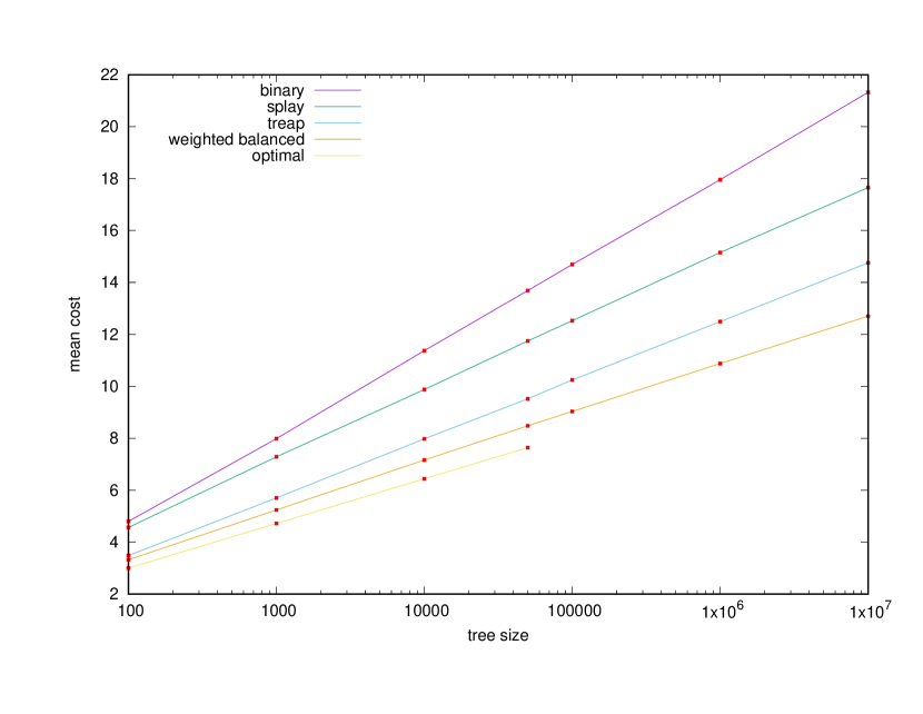
Figure 1: : Baseline performance

All experiments used 500 samples for each size considered, and the basic results appear in Figure 1. Tree size is on the $x$-axis using a log scale, and the average number of node expansions during a single (assumed to be successful) search is on the $y$-axis.

The curves in the legend are ordered from worst to best; simple binary trees perform the worst (not surprisingly), followed by splay trees, followed by treaps, and weight-balanced binary trees perform the best. Expected cost is essentially linear in the log of the size of the search tree, as one might expect.

3 Technique

We now turn to our new idea, which is simply to hill climb using rotations to improve the expected cost of the tree.

Definition 3.1

Let $T$ be a tree. $T$ will be called weighted if there is a function $p:T\rightarrow\hbox to0.0pt{\rm I\hss}\,{\rm R}$ that assigns a weight to each node in $T$ and for which $\sum_{x\in T}p(x)=1$.

If $x\in T$ is not the root of $T$, we will denote the parent of $x$ by $\pi(x)$.

We will use $\emptyset$ as a placeholder for a node that is not in $T$. So, for example, we take $\pi(x)$ to be $\emptyset$ if $x$ is the root of the tree.

If $T$ is binary and $x\in T$, we denote the left child of $x$ by $l(x)$ and the right child of $x$ by $r(x)$. Thus $x$ is a fringe node if $l(x)=r(x)=\emptyset$. We denote the sibling of $x$ by $\sigma(x)$.

For a node $x\in T$, we will define the depth of $x$, to be denoted by $d(x)$, to be $d(\emptyset)=0$ and $d(x)=1+d(\pi(x))$ otherwise.

Given a weighted tree $T$, the cost of $T$, to be denoted $c(T)$, will be defined to be

$$c(T)=\sum_{x\in T}d(x)p(x).$$

One additional property that will be of interest to us is a node that is either the left child of the left child of its grandparent, or the right child of the right child of its grandparent.

Definition 3.2

Let $T$ be a binary tree, and $x\in T$ not the root node. We will define the like-minded child of $x$, to be denoted by $\lambda(x)$, to be:

$$\lambda(x)=\cases{l(x),&if $x=l(\pi(x))$;\cr r(x)&if $x=r(\pi(x))$.}$$

Many algorithms manipulate binary trees via what are known as rotations. As an example, if $T$ is of the form shown in Figure 2, where each of $c$, $d$ and $e$ may be the roots of further subtrees, the result of operating on $T$ with a right rotation is the new tree shown in Figure 3.

Figure 2:  

Figure 3:  

Note that the new tree retains the ordering of the original (presumably $c<b<d<a<e$), and that $c$, $d$ and $e$ remain apparent fringe nodes in the new tree so that if they are in fact the roots of subtrees, those subtrees can remain attached as previously. The rotation here is generally referred to as the right rotation rooted at $a$, where $a$ is the root of the subtree being rotated.

Similarly, we will say that a left rotation at $b$ produces Figure 2 from Figure 3.

Definition 3.3

Let $T$ be a tree, and let $x\in T$ be a non-root node. By the result of bumping $x$ in $T$, to be denoted by $T^{x}$, we will mean the result of right rotating $T$ at $\pi(x)$ if $x$ is the left child of $\pi(x)$, and the result of left rotating $T$ at $\pi(x)$ if $x$ is the right child of $\pi(x)$. If $r$ is the root of $T$, we will take $T^{r}$ to be $T$ itself.

Thus Figure 3 shows the result of bumping $b$ in Figure 2, and Figure 2 is the result of bumping $a$ in Figure 3.

Recall that we are assuming that for any particular node $x\in T$, the weight $p(x)$ is the probability that $x$ is the target of a randomly selected search query. The essential point underlying our ideas is that the impact of bumping $x\in T$ can be computed exactly based purely on values of a handful of nodes surrounding $x$.

Definition 3.4

For a node $x$ in a tree $T$, we will denote by ${\overline{x}}$ the subtree of $T$ rooted at $x$. We will denote by ${\overline{p}}(x)$ the aggregated weight of the points in ${\overline{x}}$:

$${\overline{p}}(x)=\sum_{y\in{\overline{x}}}p(y).$$

We take $\overline{\emptyset}=\emptyset$ (the empty set), and thus ${\overline{p}}(\emptyset)=0$.

Proposition 3.5

Let $T$ be a weighted binary tree, and $x$ a non-root node in $T$. Then

$$C(T)-C(T^{x})=p(x)+{\overline{p}}(\lambda(x))-p(\pi(x))-{\overline{p}}(\sigma(x))$$ (1)

Proof. This is clear. Examining Figures 2 and 3, we see that the node $b$ has its depth reduced by 1, reducing the expected cost of a lookup by $p(b)$; the node $a=\pi(b)$ has its depth increased by 1. The entire subtree rooted at $c=\lambda(b)$ has its depth decreased by 1, reducing the cost by ${\overline{p}}(\lambda(b))$ while the subtree rooted at $e=\sigma(b)$ has its depth increased by 1. Right bumps are similar, and (1) follows.  

Definition 3.6

We will refer to the quantity in (1) as the merit of bumping $x$, denoting it by $\mu(x,T)$, or simply by $\mu(x)$ if no ambiguity is possible.

If $T$ is a weighted binary tree, we will say that the result of bumping $T$, to be denoted $\beta(T)$, is:

$$\beta(T)=\cases{\{T\},&if $\mu(x,T)\leq 0$ for all $x\in T$;\cr\{T^{x}|\mu(x,T)\mbox{is maximal}\},&if $\mu(x,T)>0$ for some $x\in T$.}$$

For an integer $k\geq 0$, we define $\beta^{k}(T)$ recursively by $\beta^{0}(T)=\{T\}$ and

$$\beta^{k}(T)=\cup_{t\in\beta^{k-1}(T)}\beta(t)$$

The notation would be somewhat simpler (but less precise) if we either assumed there to be a unique $x\in T$ for which $\mu(x)$ was maximal, or allowed $\beta(T)$ to be the result of bumping $T$ by an arbitrarily selected $x$ if multiple choices were available.

Since we only bump trees at nodes that have positive merit, we immediately have:

Lemma 3.7

Let $T$ be a weighted binary tree and $T^{\prime}$ any element of $\beta(T)$. Then $c(T)\geq c(T^{\prime})$, with equality if and only if $\beta(T)=T$.  

Proposition 3.8

Let $T$ be a weighted binary tree. Then there is some finite $k$ such that $\beta^{k+1}(T)=\beta^{k}(T)$.

Proof. The result will hold for any $k\geq N$, where $N$ is the total number of binary trees of the given size. Since each tree has a fixed associated cost, there can be no sequence of properly increasing costs (as per the lemma) of size greater than $N$.  

Proposition 3.9

Let $T$ be a weighted binary tree of size $n$. Then if $k$ is a positive integer, an element of $\beta^{k}(T)$ can be found in time

$$O((n+k)\log(\min(n,k))).$$

Proof. The result will follow from the following:

1. It is possible to compute both ${\overline{p}}(x)$ and $\mu(x)$ for all $x\in T$ in time $O(n)$ in an initialization phase, along with

2. A list of at least $\min(n,k)$ nodes, sorted by merit, that can be initialized in time $O(n\log(\min(n,k)))$,

3. When a node is bumped, it is possible to update the various ${\overline{p}}(x)$ and $\mu(x)$ in time $O(1)$, and

4. It is possible to update the merit-sorted list of nodes in time $O(\log(\min(n,k)))$.

The proposition then follows immediately, since the running time is $O(n+n\log(\min(n,k)))$ for the initialization and $O(1+\log(\min(n,k)))$ for each of $k$ iterations. The total running time is thus as described in the statement of the proposition.

1. ${\overline{p}}$ can be computed for all of the nodes in the tree in time $O(n)$ by simply working back from the fringe. $\mu$ can then be computed, also in time $O(n)$, by virtue of Proposition 1.

2. Given merits for all of the nodes, the $k$ highest-merit nodes can be found in time $O(n\log k)$. If $k>n$, it suffices to simply sort the merits, so that the time is therefore $O(n\log(\min(n,k)))$.

3. Consider Figures 2 and 3. When a node $x$ is bumped, the value of ${\overline{p}}(x)$ will change only for $x$ itself, since its parent is now a child, and $x$’s parent $\pi(x)$, since both $x$ and one of the subtrees rooted at a child of $x$ are no longer descendants of $\pi(x)$. Computing ${\overline{p}}(z)$ for each of these two nodes takes constant time.

   Similarly, $\mu(z)$ changes only for the nodes labeled $a$ through $e$ in the figures. Again, the update takes constant time.

4. When the merits are recomputed, inserting any new positive values into the list of nodes to bump takes time $O(\log s)$, where $s$ is the size of that list, with $s\leq\min(n,k)$ as a result. Note that we don’t need to search the entire tree for a node to “replace” the one that was just bumped; if we only plan on bumping $k$ nodes in total, we will be interested in one fewer node on the next iteration.  

4 Experimental results

It follows from the results of the previous section that we can use our ideas to reduce the expected cost of searching a binary tree, and that doing so can be done in a timely fashion. It is not clear, of course, whether the methods will be effective in practice.

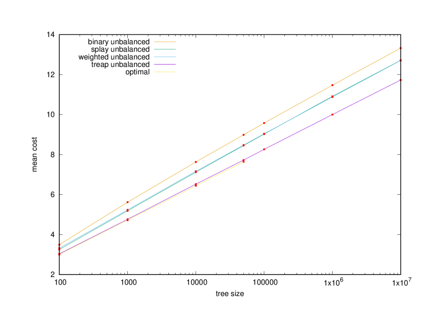
Figure 4: : Algorithm performance after unbalancing the trees

For each of the four basic tree constructions described in Section 2, we bumped nodes with the highest merit until quiescence, so that the tree could not be improved further with our simple method. The results are shown in Figure 4.

Two immediate observations are that the cost remains essentially linear in the logarithm of the tree size, and that the techniques we have proposed are by no means a panacea. They work well for some trees and clearly less well for others. Balanced binary trees, for example, provided the worst performance both before and after the trees are unbalanced.

Beyond that, however, the results are more interesting. Unbalanced splay trees and unbalanced weight-balanced trees perform virtually identically, even though their performance was starkly different before unbalancing. (In actuality, the weight-balanced trees benefited almost not at all from our ideas; the splay trees improved substantially.)

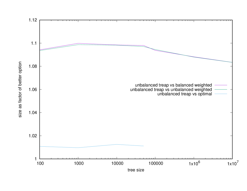
Figure 5: : Comparative performances

Perhaps more surprising is that after unbalancing, the treaps have become easily the most effective method, and their performance is very nearly optimal for all tree sizes. As shown in Figure 5, the approximately 9–10% improvement optimization (relative to either weight-balanced trees or their unbalanced versions) will provide computationally meaningful savings in practice; the 1% difference between the unbalanced treaps and optimal trees is much less interesting.

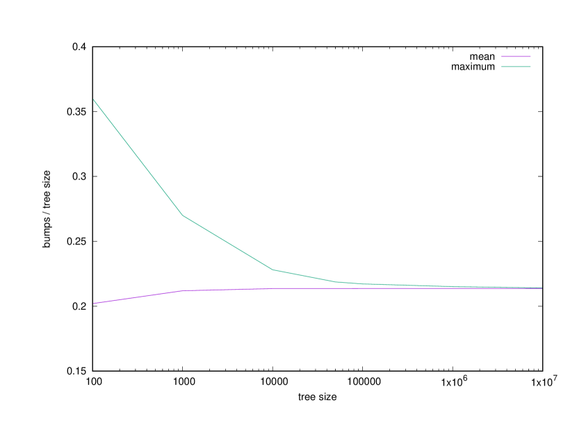
Figure 6: : Mean and maximum number of bumps, as a fraction of tree size

Of course, given the weak bounds on the number of possible bumps before quiescence, our methods might not be viable in practice after all. Data regarding this (for unbalancing treaps, which appears to be the situation of interest) appears in Figure 6. For each size tree, we show both the mean number of bumps improving a treap of that size, and the maximum number of bumps. As can be seen, both numbers stabilize at $b\approx 0.21n$, where $b$ is the number of bumps. It follows from Proposition 3.9 that the optimized tree can be found in time $O(n\log(n))$, a complexity identical to the cost of building the tree in the first place.

Figure 7: : A tree that cannot be locally optimized

Before concluding, we should expand slightly on our earlier remark that our ideas are not a panacea; consider the tree in Figure 7 where the nodes are labeled with their respective probabilities..

This tree is locally optimal under rotation, since either a left or right rotation will move one high probability node up and the other down (for no net benefit), but move the low probability node down for a net loss. The optimal tree, which has one high probability node at the root and the other at depth 1, cannot be reached in a single rotation from the tree in the figure.

5 Conclusion and future work

The techniques that we have described appear to lead to clear and measurable improvements in access times for binary trees, but only scratch the surface of potential applications. Some obvious candidates for future work:

Non-binary trees

There is no reason to restrict our ideas to binary trees; any data structure where a similar measure of merit can be computed locally should be amenable to similar treatment.

Unbalancing restrictions

It is possible to apply additional constraints when selecting a node to bump. As an example, if we begin with a binary tree where the maximum node depth is $d$, we could require that no node can be bumped if it pushes another node below depth $d$. This would lead to guaranteed performance improvements with no impact on worst-case performance. We could also obviously limit the maximum depth of a post-bump node in some less restrictive way. Since it is possible to compute and maintain $d({\overline{x}})$ for each node $x$, the impact on computational expense should be minimal.

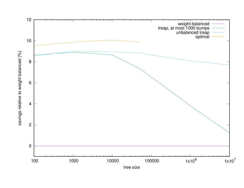
Figure 8: : Impact of limiting the number of bumps

Termination before quiescence

Alternatively, one could limit the number of bumps to be a sublinear function of tree size in some way, although this may be difficult without significantly impacting performance. Figure 8, for example, shows performance both for optimized treaps and for treaps where at most 1000 bumps were permitted before the optimization was stopped. As can be seen, allowing our methods to proceed until quiescence provides significant improvement without changing the overall complexity of constructing the tree. Of course, we have no guarantee that the number of bumps will be linear in tree size, and we could obviously limit the number of bumps to (say) 50% of the number of nodes in the tree. Given the “maximum” curve in Figure 6, doing so would not impact any of the results we have presented.

Multiple bumps

One can imagine situations where bumping a node once degrades overall performance, but bumping it twice provides an improvement. In general, updating the merits after a single bump involves recomputing values for 5 nodes; updating the merits after a bump of $l$ levels will involve recomputing values for $2l+3$ nodes.

It follows that as long as the depth of the tree is bounded at some fixed multiple of $\log(n)$, we can consider not just single bumps but bumps of any number of levels and only add a factor of $\log(n)$ to the worst-case running time. Of course, given that we are producing trees with search costs within 1% of optimal, the additional complexity of such considerations may not be warranted.

Testing all of these ideas should be straightforward.

Conflict of interest

Funding:

Not applicable.

Conflicts or competing interest:

None.

Availability of data, material and code:

Code and other materials will be provided upon request. The author reserves the right to patent the techniques described here. In the event that such patents are filed and granted, publication of this paper carries with it a permanent, royalty-free license for noncommercial use of the technology herein described.

References

- (1) Adamic, L., Huberman, B.: Zipf’s law and the internet. Glottometrics 3 (2001)
- (2) Aragon, C.R., Seidel, R.: Randomized search trees. In: Proc. 30th Symp. Foundations of Computer Science (FOCS-89), pp. 540–545. IEEE (1989)
- (3) Breslau, L., Pei Cao, Li Fan, Phillips, G., Shenker, S.: Web caching and Zipf-like distributions: Evidence and implications. In: Proc. Eighteenth Annual Joint Conference of the IEEE Computer and Communications Societies. The Future is Now (Cat. No.99CH36320), vol. 1, pp. 126–134 vol.1 (1999)
- (4) Cunha, C., Bestavros, A., Crovella, M.: Characteristics of www client-based traces. Tech. rep., Boston University, USA (1995)
- (5) Demaine, E.D., Harmon, D., Iacono, J., Kane, D., Patrascu, M.: The geometry of binary search trees. In: Proc. 20th Ann. ACM-SIAM Symp. on Discrete Algorithms (SODA-09), pp. 496–505. ACM (2009)
- (6) Garsia, A.M., Wachs, M.L.: A new algorithm for minimum cost binary trees. SIAM J. Comput. 6, 622–642 (1977)
- (7) Hu, T., Tucker, A.: Optimal computer search trees and variable-length alphabetical codes. SIAM J. Applied Math. 21, 514–532 (1971)
- (8) Karpinski, M., Larmore, L.L., Rytter, W.: Sequential and parallel subquadratic work algorithms for constructing approximately optimal binary search trees. In: Proc. 7th Ann. ACM-SIAM Symp. on Discrete Algorithms (SODA-96), pp. 36–41. ACM (1996)
- (9) Karpinski, M., Larmore, L.L., Rytter, W.: Correctness of constructing optimal alphabetic trees revisited. Theor. Comp. Sci. 180, 309–324 (1997)
- (10) Knuth, D.E.: The Art of Computer Programming 3: Sorting and Searching, chap. 6, pp. 400,436–453. Addison-Wesley, Upper Saddle River, NJ (1998)
- (11) Lecomte, V., Weinstein, O.: Settling the relationship between Wilber’s bounds for dynamic optimality. Tech. rep., Columbia University, USA (2019). ArXiv:1912.02858
- (12) Mehlhorn, K.: Nearly optimal binary search trees. Acta Informatica 5, 287–295 (1975)
- (13) Mehlhorn, K., Tsagarakis, M.: On the isomorphism of two algorithms: Hu/Tucker and Garsia/Wachs. In: Les arbres en algèbre et en programmation (4ème Colloq.), pp. 159–172 (1979)
- (14) Nagaraj, S.: Optimal binary search trees. Theor. Comp. Sci. 188, 1–44 (1997)
- (15) Prisco, R.D., Santis, A.D.: New lower bounds on the cost of binary search trees. Theor. Comp. Sci. 156, 315–325 (1996)
- (16) Seidel, R., Aragon, C.R.: Randomized search trees. Algorithmica 16, 464–497 (1996)
- (17) Sleator, D.D., Tarjan, R.E.: Self-adjusting binary search trees. J. of the ACM 32, 652–686 (1985)
- (18) Zipf, G.: Selected Studies of the Principle of Relative Frequency in Language. Harvard University Press (1932)