Exploiting stellar explosion induced by the QCD phase transition in large-scale neutrino detectors
Abstract
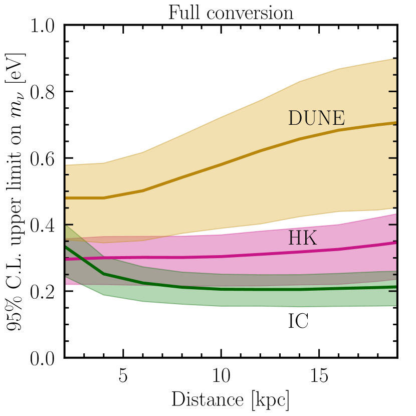
The centers of the core-collapse supernovae are one of the densest environments in the Universe. Under such conditions, it is conceivable that a first-order phase transition from ordinary nuclear matter to the quark-gluon plasma occurs. This transition releases a large amount of latent heat that can drive a supernova explosion and may imprint a sharp signature in the neutrino signal. We show how this snap feature, if observed at large-scale neutrino detectors, can set competitive limits on the neutrino masses and assist the localization of the supernova via triangulation. The 95%C.L. limit on the neutrino mass can reach 0.16 eV in Ice-Cube, 0.22 eV in Hyper-Kamiokande, and 0.58 eV in DUNE, for a supernova at a distance of 10 kpc. For the same distance and in the most optimistic neutrino conversion case, the triangulation method can constrain the angular uncertainty of the supernova localization within in the considered pairs of the detectors, leading to an improvement up to an order of magnitude with respect to the often considered in the literature rise time of the neutronization burst.
I Introduction
The detection of electron antineutrinos from SN 1987A Hirata et al. (1987); Bionta et al. (1987); Alexeyev et al. (1988) was a significant milestone in multimessenger astronomy. It provided direct evidence that, in their latest stages of life, massive stars emit a considerable fraction of the gravitational binding energy in the form of neutrinos. Many aspects of core-collapse supernovae (CCSNe) are well investigated (for recent reviews see, e.g, Refs. Janka (2017); Burrows and Vartanyan (2021)). During the infall phase each element of matter moves with constant entropy Brown et al. (1982). After reaching sufficiently high densities, electrons get captured on heavy nuclei and protons, producing an initial sharp burst of electron neutrinos with typical luminosities of the order few erg Bethe et al. (1979); Fuller et al. (1982). This is followed by a smooth signal of neutrinos of all flavors created primarily by pair-production processes during the accretion and cooling of the newly formed protoneutron star Mirizzi et al. (2016); Horiuchi and Kneller (2018).
There are several questions regarding CCSNe that remain unanswered. One unsettled crucial issue is the mechanism by which CCSNe explosions occur. The most widely explored hypothesis is the delayed neutrino heating mechanism Colgate and White (1966); Bethe and Wilson (1985). This scenario, in a simplified fashion, can be explained in the following way: after the core bounce, the stalled shock wave is revived by an increase in thermal pressure due to reabsorption (neutrino heating) of a fraction of the neutrinos emitted (neutrino cooling) from the protoneutron star. In reality, the process of neutrino decoupling from the matter, which dictates the neutrino heating and cooling rates, is a complex phenomenon determined by the neutrino absorption, emission, and scattering reactions with the matter Raffelt (2001); Fischer et al. (2012). The neutrino heating aids in the development of hydrodynamical instabilities Blondin et al. (2003); Tamborra et al. (2014); Couch and Ott (2015); Abdikamalov et al. (2015) which in turn have been shown to produce explosions in many of the state-of-the-art three-dimensional supernova simulations. However, these models only explode for stars with masses below approximately and do not produce large explosion energies (hypernovae) Galama et al. (1998); Stanek et al. (2003); Hjorth et al. (2003); Della Valle et al. (2006).
Besides neutrino heating, other explosion mechanisms have also been proposed, e.g., magnetorotational supernova mechanism LeBlanc and Wilson (1970); Takiwaki et al. (2009); Mösta et al. (2015); Obergaulinger and Aloy (2021); Matsumoto et al. (2022), the acoustic mechanism Burrows et al. (2006); Gossan et al. (2020), and sterile neutrino decays Fuller et al. (2009); Rembiasz et al. (2018); Mastrototaro et al. (2020) and conversions Qian et al. (1993); Sigl (1995); Hidaka and Fuller (2006); Suliga et al. (2020). One of the most notable of them is the quark-hadron phase transition (QHPT) mechanism Sagert et al. (2009); Fischer et al. (2011, 2018); Zha et al. (2021); Fischer (2021); Kuroda et al. (2022); Bauswein et al. (2022); Lin et al. (2022); Jakobus et al. (2022) in which the stellar explosion is connected with a first-order phase transition from nuclear to quark matter. The latent heat released during the transition can launch a second shock wave which can help drive the explosion. As this fast shock passes the neutrinosphere, a sharp burst containing mostly electron antineutrinos is released. The detection of such a sharp feature in the neutrino signal would not only strongly support the occurrence of the phase transition in SN cores but also enable testing the physics affecting neutrino propagation.
In this work, we show that the detection of the QHPT peak in neutrino signal by the three existing and future large-scale detectors – Ice-Cube Halzen and Raffelt (2009), Hyper-Kamiokande Abe et al. (2018), and DUNE Abi et. al. (2020) – can set competitive limits on neutrino masses and can greatly improve the precision of localization of the supernova Dasgupta et al. (2010). Two effects make this feasible – the sharpness and intensity of the QHPT peak.
This paper is organized as follows; in Sec. II we briefly describe the supernova explosion mechanism due to QHPT, show the nominal neutrino signal expected from the QHPT, and discuss the impact of neutrino conversions inside the star on the neutrino propagation through the supernova medium. In Sec. III we summarize the status of supernova triangulation and the limits on neutrino masses, and show how they can be improved by employing the rise time of the sharp signal feature. Sections IV and V describe the detectors employed in our work and the results obtained, respectively. Finally, we summarize and discuss our results in Sec. VI.
II Neutrino signal from QCD Phase Transition Supernova
In this section, we review the supernova explosion mechanism due to a quark-hadron phase transition (Sec. II.1) and highlight how it compares to neutrino fluxes without such transition (Sec. II.2). In short, the QHPT produces an additional narrow peak in the neutrino signal during the accretion phase, as we elaborate below.
II.1 Quark-hadron phase transition as an engine for supernova explosion
When a star with a mass M⊙ has reached the end of its life and its core has attained sufficiently high densities, the photodisintegration of heavy nuclei as well as electron captures on nuclei and free protons reduce the pressure in the inner core and eventually lead to collapse on a dynamical timescale Janka (2017). Electron captures produce a huge amount of electron neutrinos that get trapped inside the core once the central density exceeds few g cm-3 Bethe et al. (1979).
In the remaining collapse when nuclear saturation densities of about are reached, the collapse is halted by the repulsive short-range nuclear forces, leading to a stiffening of the equation of state (EoS) and a (first) core bounce. A protoneutron star (PNS) is left at the center of the star and a shock wave is launched. As the shock crosses the neutrinosphere, the neutronization burst of electron neutrinos is released. The neutrino losses and continuous energy loss due to the dissociation of in-falling of heavy nuclei from the outer core quickly cause the shock to stall Bethe (1990); Woosley et al. (2002).
The following evolution of the EoS and shock wave determine whether the star explodes and what kind of a compact remnant is formed, a black hole (BH), a neutron star (NS), or another kind of compact star containing nonhadronic matter Gerlach (1968); Alford et al. (2013); Espino and Paschalidis (2022). Given that the state of matter at densities well exceeding the nuclear saturation density is highly uncertain, the question about the composition of the central object is not unsubstantiated.
The possibility of a phase transition between the hadronic and quark matter has been studied extensively in the context of CCSNe Migdal et al. (1979); Takahara and Sato (1988); Gentile et al. (1993); Pons et al. (2001); Drago et al. (2008); Nakazato et al. (2008); Sagert et al. (2009); Fischer et al. (2011, 2018); Zha et al. (2021); Fischer (2021); Kuroda et al. (2022); Bauswein et al. (2022); Lin et al. (2022); Jakobus et al. (2022). In several cases, it has been found that close to saturation density, for high temperatures and low proton fractions, the phase transition can occur in the early postbounce phase of a CCSN. In such cases, the accelerated contraction of the PNS in the mixed quark-hadron phase may lead to development of a pure quark phase. The associated stiffening of the EoS causes an abrupt halt of further contraction; a second strong shock wave forms, which can merge with the initial stalled bounce shock and trigger the SN explosion Sagert et al. (2009).
The QHPT provides an alternative mechanism for a successful SN explosion. It has also been shown to create explosions for otherwise nonexploding SN models Fischer et al. (2018). Moreover, the propagation of the second shock across the neutrinospheres releases an additional ms burst of neutrinos. Such a burst is dominated by because matter in PNS is neutron rich, and in the presence of a large abundance of positrons due to high temperatures achieved during the shock propagation positron capture dominates over electron capture, favoring production of over , and . We investigate the value of detecting this sharp feature in the SN neutrino signal in the remaining of our work.
II.2 Numerical model
For our benchmark QHPT SN neutrino signal, we use the results from a one-dimensional general-relativistic radiation-hydrodynamical simulation with Boltzmann neutrino transport from Ref. Fischer et al. (2018) of a 50 CCSN progenitor evolved using the AGILE-BOLTZTRAN tool Liebendoerfer et al. (2004); Mezzacappa and Bruenn (1993); a hadron-quark hybrid EoS where deconfinement is taken into account via an effective string-flip potential was developed for the simulation Fischer et al. (2018) based on Refs. Bastian (2021); Kaltenborn et al. (2017). The developed EOS is within approximately 95%C.L. region constraints from combining the gravitational wave observation of the binary neutron star merger and X-ray plus radio observations of the pulsars Riley et al. (2021); Raaijmakers et al. (2021). The used model results in a successful explosion with an energy approximately erg at the shock breakout.
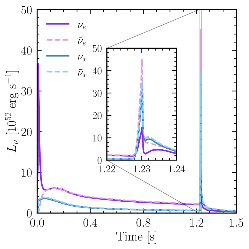
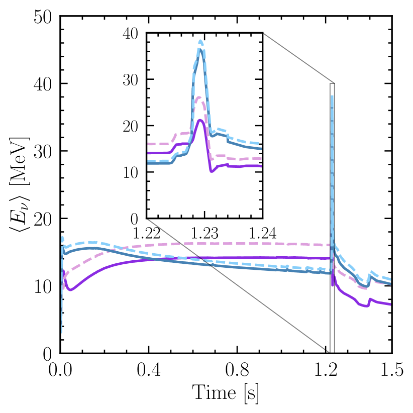
Figure 1 shows the temporal evolution of neutrino luminosities (left panel) and average energies (right panel) from the employed QHPT SN model Fischer et al. (2018). At early times one can see the neutronization burst of neutrinos released after the core bounce. At around s, after the creation of the pure quark matter phase, the second hydrodynamical shock takes over the standing bounce shock and triggers the onset of the SN explosion Fischer et al. (2018). A few tens of milliseconds later (around s) the shock reaches the neutrinosphere and a second millisecond burst of is released. Comparing its duration to the neutronization burst, the QHPT burst is much sharper Sagert et al. (2009); Fischer et al. (2011, 2018), with the width related to the energetics of the second shock. In addition, as the QHPT shock travels through the neutrinospheres and heats up the matter, the mean neutrino energies increase sharply analogously to the luminosities.
II.3 Neutrino spectra
To construct the neutrino fluxes from the QHPT SN, we assume that the outgoing neutrino spectra obey Fermi-Dirac distributions with negligible chemical potential, since the amount of spectral pinching in the signal after the neutronization phase is expected to be small as compared to the neutronization burst phase Janka (2017); this is also true for the QHPT CCSN model we use, where the pinching parameter () during the burst varies between 2 and 4. These distributions can be easily recovered using the parametrization form Keil et al. (2003); Keil (2003); Tamborra et al. (2012),
| (1) |
where is the neutrino energy, is the average neutrino energy, and the normalization factor . The pinching parameter for the Fermi-Dirac distribution is . Finally, the differential flux of neutrinos (, where indicates or , as to first order they are indistinguishable for the purposes of supernova modeling) can be obtained as follows:
| (2) |
where is the luminosity of neutrino flavor , and is the distance to the SN.
II.4 Neutrino flavor conversion in dense medium
While propagating through the SN medium, neutrinos undergo flavor conversions due to their self-interactions and coherent forward scattering of the medium particles. The former is a highly nonlinear phenomenon subject to numerous ongoing studies aiming to understand its impact on the neutrino flavor evolution (see, e.g., Refs. Duan et al. (2010); Chakraborty et al. (2016); Tamborra and Shalgar (2020); Patwardhan et al. (2021) and references therein). The latter effect leads to the well-known Mikheyev-Smirnov-Wolfenstein (MSW) resonance effects, experimentally observed for solar neutrinos Wolfenstein (1978); Mikheev and Smirnov (1986). As a result of the MSW conversions, neutrino eigenstates change their flavor reflecting the changes in the density of electrons they traveled through.
In order to take into account all the uncertainties related to the flavor transformation in the dense stellar environment, in this work we consider two extreme conversion scenarios, i.e., the no conversion case and full conversion between and ( and ). In the case of electron neutrino detectors, this should coincide with the maximal variation in the uncertainty on the parameters of interest. For electron antineutrino detectors, however, that might not be the case, as although the luminosity of is larger than the one, the mean energies display the opposite behavior (see Fig. 1). In Sec. V we show that for electron antineutrino detectors, the no conversion scenario yields the best results.
III EXPLOITING THE SHARP FEATURE OF THE NEUTRINO SIGNAL
In this section, we outline how the observation of the QHPT peak in the neutrino signal can be used to improve the localization of the supernova in the sky (Sec. III.1) and constrain the absolute neutrino mass (Sec. III.2).
III.1 Triangulation
Since neutrinos interact weakly with matter, they escape almost unimpeded from the extremely dense regions of an exploding SN, making them the first messengers to inform us of the occurrence of the gravitational collapse. Due to their frequent interactions with the star’s envelope, photons emerge more slowly with an hours to days delay compared to neutrinos Nakamura et al. (2016). In addition, the electromagnetic radiation might be obscured by dust surrounding the star as well as the interstellar medium or be absent for stars directly forming BHs. In such cases observing neutrinos may be the only way to obtain the information about the SN, apart from the possible simultaneous detection of gravitational waves Antonioli et al. (2004); Pagliaroli et al. (2009); Warren et al. (2020); Pajkos et al. (2021); Halim et al. (2021). Any prompt information about the SN direction represents a valuable tool to alert astronomers and allow for a rapid multimessenger follow-up.
Two types of localization techniques have been considered for SN neutrinos. The first one uses an individual detector for pointing and is based on angular distributions of neutrino-matter interaction products, which can be correlated with the neutrino direction. In this case, a single experiment can independently determine the SN direction and its uncertainty. One of the most considered channels is neutrino elastic scattering on electrons, which is a highly anisotropic interaction Beacom and Vogel (1999); Tomas et al. (2003). The outgoing electron is scattered in the direction of the incoming neutrino momentum, allowing detectors with sufficient spatial resolution to reconstruct the direction of the neutrino source. As a reference, pointing with elastic scattering in Hyper-Kamiokande may reach precision of 1∘-1.3∘ Abe et al. (2018).
In the context of multimessenger astronomy, it is always a good practice to use as much information as possible. In this regard, the complementary method that has been considered is triangulation Beacom and Vogel (1999); Mühlbeier et al. (2013); Brdar et al. (2018); Hansen et al. (2020); Linzer and Scholberg (2019); Coleiro et al. (2020); Sarfati et al. (2022), which is based on measuring the arrival time delay between pairs of widely separated detectors around the globe. Such technique requires an immediate sharing of data among the different experiments.
Past works on this subject have focused on two features of the neutrino signal, the neutronization burst Beacom and Vogel (1999); Scholberg et al. (2010); Mühlbeier et al. (2013); Brdar et al. (2018); Hansen et al. (2020); Linzer and Scholberg (2019); Coleiro et al. (2020) and the signal demise at BH formation Mühlbeier et al. (2013); Brdar et al. (2018); Hansen et al. (2020); Sarfati et al. (2022). The key property shared by these features is their swift change in the number of neutrinos. During the neutronization burst, the electron neutrino signal sharply increases over a tens of ms timescale, whereas a rapid cutoff of neutrinos in the span of few ms follows the BH formation.
Our work seeks to test the feasibility of using the neutrino flux peak caused by the QHPT to time the neutrino signal in an effort to triangulate a SN. The advantage of this approach over using the neutronization burst is that the QHPT peak has a much shorter rise time, on the order of ms. It also does not rely on the SN creating a BH to produce a neutrino cutoff, which occurs an estimated 10%-40% of the time based on theory Ertl et al. (2016); Couch et al. (2020); Sukhbold et al. (2016) and observations Adams et al. (2017a, b); Neustadt et al. (2021) and may suffer from gravitational redshift softening the cutoff for black hole formation Wang et al. (2021).
III.2 Absolute neutrino mass
While the observation of neutrino oscillations confirmed the existence of nonzero neutrino masses Fukuda et al. (1998); Hirata et al. (1992); Bellerive et al. (2016), from the oscillation experiments alone we can only learn about the squared mass differences. The measured squared mass splittings, however, do set the lower limit on neutrino masses assuming that the lightest neutrino mass state is massless. In the case of normal ordering (NO) it is , whereas for the inverted ordering (IO) , where denotes the active neutrino mass state index.
The strongest upper limit on the sum of the neutrino masses comes from cosmological observations and is approximately Zyla et al. (2020). While it may be tempting to consider this value as a strong hint for NO, these limits vary with various assumptions about the employed statistical procedures (see, e.g., Refs. Gariazzo et al. (2018); Jimenez et al. (2022); Chudaykin et al. (2022); Gariazzo et al. (2022)). Terrestrial experiments can also set upper limits on the neutrino mass based on energy and momentum conservation. The most stringent limit comes from the Karlsruhe Tritium Neutrino experiment (KATRIN) Angrik et al. (2005), which looks at the end point of the electron spectrum from beta decay of tritium, and is eV Aker et al. (2022).
The existence of nonzero neutrino masses is not without consequences for neutrinos produced in CCSNe. It not only facilitates neutrino conversions but also introduces energy-dependent time delays in the neutrino flux arriving at the Earth Zatsepin (1968). The delay of a neutrino mass state () with energy () can be calculated as
| (3) |
where is the distance to the SN. The detection of a neutrino signal from a nearby SN can then be used to set limits on the neutrino masses Zatsepin (1968). The observation of neutrinos from SN 1987A set the mass limit of at 95% C.L Loredo and Lamb (2002); Pagliaroli et al. (2010), where all three active neutrino mass states are assumed to have the same mass because the mass squared differences are much smaller than this limit.
The limits coming from a detection of neutrinos from a future CCSN calculated with different techniques (e.g., functional fit to the signal or timing first neutrino event with the gravitational wave signal) and detectors vary between approximately Nardi and Zuluaga (2004, 2005); Pagliaroli et al. (2010); Lu et al. (2015); Rossi-Torres et al. (2015); Hansen et al. (2020); Pompa et al. (2022) for the benchmark distance to the SN of 10 kpc. The limit is expected to be significantly more stringent than the one from SN 1987A neutrinos, mostly thanks to improvements in the detection of MeV-energy neutrinos from SN Scholberg (2012); Al Kharusi et al. (2021).
In addition, using the sharp end of the neutrino signal in case of BH formation sets a limit on the neutrino mass of , again depending not only on the type and volume of the considered detectors Beacom et al. (2000); Hansen et al. (2020) but also on the decay length of the signal. The latter is determined by the environment where the BH formation occurs. In cases where the accretion flow cannot be neglected Gullin et al. (2022) it prolongs the neutrino signal causing the obtained mass limit to weaken.
In this work, we investigate the feasibility of employing the neutrino burst from QHPT SN in setting the upper limits on the absolute neutrino mass. Given the sharpness of the QHPT peak, we expect that the observation of such signal in large-scale neutrino detectors will result in a more stringent limit on the neutrino mass than the one obtained from the detection of the neutronization burst.
We note that there also have been works investigating the possibility of determining the neutrino mass ordering with the neutronization rise time Serpico et al. (2012); Brdar and Xu (2022) assuming only the impact of neutrino interactions with matter on the conversion probabilities. Since, however, we take a conservative approach with respect to the impact of neutrino-neutrino interactions on the neutrino flavor evolution inside the supernova core (see Sec. II.4), we are not exploring this scenario.
IV Detection of the Neutrino Burst
In order to resolve the sharp peak due to QHPT, we employ three of the largest existing and upcoming neutrino experiments: Hyper-Kamiokande (HK), Ice-Cube (IC), and the Deep Underground Neutrino Experiment (DUNE), which are described shortly in Secs. IV.1 - IV.3; the characteristics and angular coordinates for the three considered detectors are summarized in Table 1.

Detector Interaction Fiducial mass Number of Energy threshold Latitude Longitude Distance between detectors channel [kt] targets [MeV] [deg] [deg] [km] IC -90 0 D HK D DUNE Ar D
In each of the three considered detectors, the energy-integrated event rate from the interaction channel can be calculated with the following formula:
| (4) |
where is the efficiency of the detector, which reflects what percentage of the detected signal can be directly translated into the event rate, is the number of targets in the detector volume, is the differential cross section for the interaction , is the threshold energy for the detector with the corresponding neutrino energy, and is the maximum energy that can be transferred to the detectable particle.
IV.1 Hyper-Kamiokande
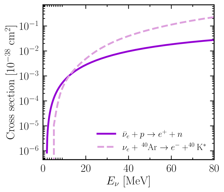
HK Abe et al. (2018), which is currently under construction in Japan, is a 217 kt water Cherenkov detector. The main detection channel for MeV-energy-range SN neutrinos is inverse beta decay (IBD): . This detection channel relies on observing the Cherenkov radiation emitted by the positron to identify the individual neutrino IBD reaction. In our work we neglect the small contribution coming from other reactions such as elastic scattering on electrons or neutral current neutrino-oxygen scattering, and focus only on the IBD channel. While it makes our analysis more conservative, it does not significantly affect the results. We compute the HK event rate using Eq. 4 with the cross section for IBD Strumia and Vissani (2003); Ricciardi et al. (2022) shown in Fig. 3 as a function of the neutrino energy, positron energy threshold 5 MeV, and 100% efficiency Abe et al. (2018). The temporal resolution of HK is expected to be of the order of ns Abe et al. (2018). According to the Ref. Linzer and Scholberg (2019) the background rate in 217 kton HK can be as large as ; however, since we are focusing on a short time window for the QHPT peak (few ms) and do not look for time differences between single events, we neglect any contribution from background events in our analysis.
IV.2 Ice-Cube
The IC neutrino observatory is an ice Cherenkov neutrino detector located at the South Pole Halzen and Klein (2010). It consists of 5160 digital optical modules (DOMs), each of a volume capable of observing MeV-energy-range neutrinos from SN through IBD Abbasi et al. (2011). While in this energy range IC cannot resolve the energy of individual neutrinos, the overall background rate will be enhanced signifying the SN signal. The temporal resolution for IC can reach down to few ns Freiherr Heereman von Zuydtwyck (2015).
To obtain the photoelectron counts in the IC detector we follow the procedure described in Ref. Abbasi et al. (2011). The total IBD event rate in the volume of the detector can be estimated with
| (5) |
where is the dead-time efficiency. With the dead time , the background noise can be reduced to the level of Abbasi et al. (2011). The IBD rate without accounting for background noise and the dead-time correction [which serves as the energy dependent efficiency () of the detector], is given by Abbasi et al. (2011)
| (6) |
where is the number of DOMs, is the density of targets in the ice, is the effective volume for a single photon, is the number of Cherenkov radiated photons by an electron with energy , and is the differential IBD cross section.
IV.3 DUNE
DUNE near and far detectors will be constructed in Batavia and South Dakota, United States Abi et. al. (2020), respectively. For the purpose of SN neutrino detection, we consider the far detector which is planned to be a 40 kton liquid argon time projection chamber. Liquid argon has a particular sensitivity to the component of a SN neutrino burst, since the main detection channel for MeV-energy neutrinos is . The observable for this channel is the plus deexcitation products from the excited final state. We use the total cross section for this charged-current reaction as reported in Refs. Abi et al. (2021); Abi et. al. (2020), obtained by simulating the interaction of MeV neutrinos with nuclei in liquid argon through the event generator MARLEY, see Fig. 3. Comparable cross section has been calculated in Ref. Suzuki and Honma (2013); Toshio Suzuki (2022). The energy-dependent detector efficiency together with the energy threshold are taken from Ref. Abi et al. (2021). DUNE can also detect and by the charged-current and neutral current interactions on argon. However, we neglect these contributions as they are suppressed by at least an order of magnitude compared to induced event rate Abi et al. (2021). The background rate in DUNE originating from solar neutrinos Capozzi et al. (2019), fast neutrons Li et al. (2021) and spallation Zhu et al. (2019) is expected to be approximately ; therefore, similarly as for HK, we neglect the contribution from the background in our analysis.
IV.4 Event rates
Figure 2 shows the total neutrino event rate in the three considered detectors IC (green lines), HK (pink lines), and DUNE (yellow lines) from the QHPT SN occurring at a distance of 10 kpc from the Earth for the no conversion (solid lines) and full conversion (dash-dotted lines) cases.
The highest event rate for DUNE is for the case of full conversion due to a higher luminosity and average neutrino energy for than (see Fig. 1). For water Cherenkov detectors, the event rates during the QHPT peak in both conversion scenarios are comparable; the larger luminosity compared to is balanced by smaller average energy of versus at the peak (see Fig. 1). During the pre-QHPT-burst phase the difference in the event rates for the two conversion scenarios is more prominent.
The event rate in DUNE is low compared to HK and IC due to the smaller detector volume and lower efficiency, especially for neutrino energies between 5-12 MeV. It is also worth noting that the event rate in the IC detector during the QHPT peak dominates the background noise, which is not the case for SN models without QHPT Abbasi et al. (2011).
In all three detectors the QHPT neutrino burst is distinguishable from a neutrino signal without such feature at approximately more than level for both conversion scenarios until a distance of kpc. Therefore, in Sec. V we limit our analyses to that distance.
V METHODS AND RESULTS
In this section we present our results on SN triangulation and limits on absolute neutrino mass from the detection of the sharp QHPT peak in the SN neutrino signal. In Sec. V.1 we summarize the method to determine the timing of the neutrino signal. Later in Sec. V.2–V.3 we show our findings for SN triangulation, while in Sec. V.4 we calculate the sensitivity to the absolute neutrino mass.
V.1 Timing the neutrino signal
The time delay recorded by different neutrino detectors can be used to infer the SN neutrino arrival direction with the triangulation method Beacom and Vogel (1999); Mühlbeier et al. (2013); Brdar et al. (2018); Hansen et al. (2020); Linzer and Scholberg (2019); Coleiro et al. (2020); Sarfati et al. (2022). In order to use this method, we first calculate the time delays between pairs of detectors and their uncertainties by fitting the rise time of the QHPT peak in the neutrino event rates (see Fig. 2).
Two factors limit the determination of the neutrino arrival time: first, the temporal resolution of the investigated detectors, and second, the theoretical uncertainty coming from the simulations’ time step size. In our case, the latter is the limiting factor; thus, we bin the event rates in 0.1 ms bins for each detector, which is of the order of the temporal resolution of the simulation’s data output in the vicinity of the neutrino peak caused by the QHPT.
Similarly, as in Ref. Halzen and Raffelt (2009), to calculate the rise time of the QHPT peak, we fit the neutrino event rates with the following linear function:
| (7) |
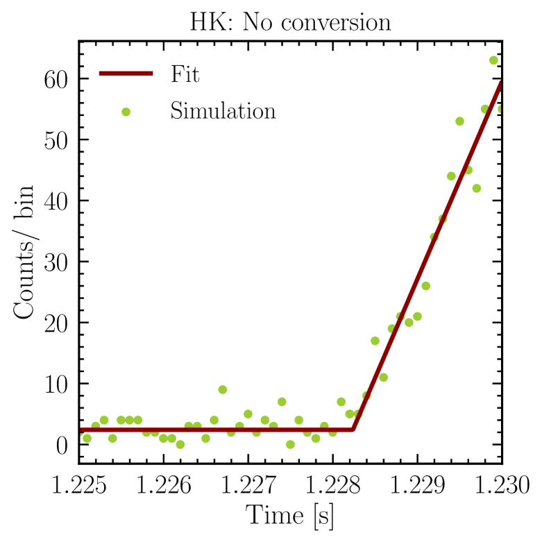
where is the flat event rate before the QHPT peak appearance, is the start time of the QHPT peak that we are determining, and is a fitting parameter. We apply the fitting function between s, where the flat signal dominates, and s, where we expect the QHPT burst to peak. Note that the choice of a linear fitting function over, for example, an exponential one, is well motivated given the sharpness of the considered signal. The upper panel of the Fig. 4 illustrates an example of the fitting procedure adopted for the HK event rate in case of no neutrino conversions.
By assuming Poisson statistics, for any combination among IC, HK, and DUNE, we generate pairs of random burst signals. This number of trials ensures negligible variations in the obtained results. For each realization, we fit the rise time of the QHPT burst in each of the two detectors and calculate the time difference between them. Such time difference, which is due only to the fact that the considered detectors are not identical under one conversion scenario, is what represents the bias in Eq. 10 (see Sec. V.2). The means and the standard deviations of the obtained in that way distributions are reported in Table 2, for the case of no conversion and full neutrino conversion. Histograms of the time distribution are also shown in Fig. 7. The difference between the rise time and its error strongly depends on the conversion scenario in case of pairing with DUNE. The latter gives the largest uncertainty, mainly due to the low statistics. Nevertheless, the full conversion scenario is still significantly better than the no conversion case, both because of a larger number of events, and a more pronounced ratio peak to preburst signal.
| Detectors | No conversion | Full conversion |
|---|---|---|
| [ms] | ||
| IC-HK | ||
| IC-DUNE | ||
| HK-DUNE | ||
| (min, max) [deg] | ||
| IC-HK | ||
| IC-DUNE | ||
| HK-DUNE | ||
| 95% C.L. upper limit on [eV] | ||
| IC | ||
| HK | ||
| DUNE | ||
V.2 The triangulation method
We have established the bias in the measurement of the rise time due the different detector properties for the set conversion scenario. Now, in order to employ the triangulation method, we compute the temporal delay between the arrival times of the neutrino pulse in different telescopes. For two detectors on Earth located at and , the recorded time delay can be expressed as:
| (8) |
where is the speed of light, the distance between the detectors listed in Table 1, and n is the unit vector that indicates the direction from which the neutrinos arrive. For a SN occurring at right ascension and declination , this vector is given by:
| (9) |
We assume that the SN is located at the galactic center with deg and deg, and the collapse happens on the vernal equinox at noon coordinate universal time (UTC). Following Refs. Linzer and Scholberg (2019); Sarfati et al. (2022) we define the total time delay as:
| (10) |
where is the bias provided in Table 2. The uncertainty on is obtained by adding in quadrature the one on and , resulting in a factor increase with respect to .
Given a time delay with an error , the uncertainty on the determination of (Eq. 8) is
| (11) |
which can be estimated as follows Beacom and Vogel (1999); Linzer and Scholberg (2019):
| (12) |
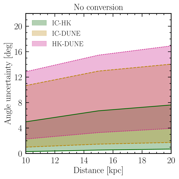
These are the two extremal angular uncertainties, the former one for large angles (up to ), and the latter for small ones ( ), which limit the determination of the SN location. Their values are reported in Table 2 for each pair of detectors for SN at a distance of 10 kpc. As opposed to no conversion, in the case of full conversion the pairing with DUNE improves significantly the pointing precision because of a smaller error on . All detector pairs provide a competitive minimum angular uncertainty if compared to using elastic scattering on electrons. The bottom panel of the Fig. 4 shows the range of angular uncertainties as a function of the distance to the SN for the case of no conversion. Due to a decrease in the number of events in all considered detectors with increasing distance to the SN the error on the determination of the SN location grows.
V.3 Combined analysis
In order to calculate the confidence regions of the SN localization in the sky, we perform a combined analysis using the results from all three detectors. Similarly as in Ref. Sarfati et al. (2022), to take into account correlations among the detectors, we construct the following function Barlow (Wiley, Chichester, 1989):
| (13) |
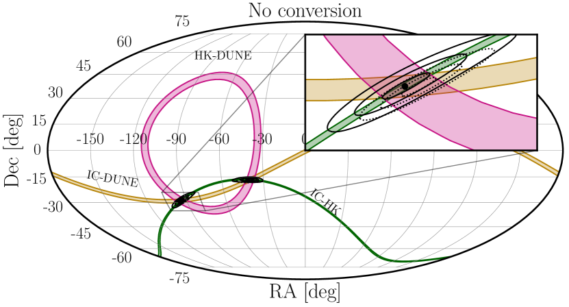
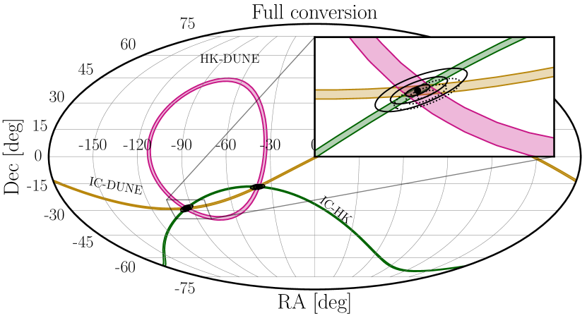
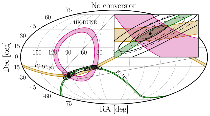
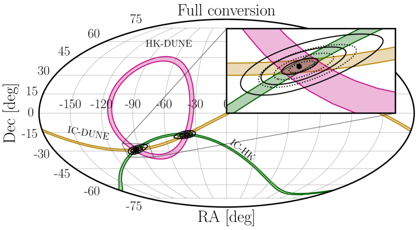
where is the theoretically expected time difference for a SN located at , is the expected measured time difference for the true SN located at as defined in Eq. 8, and the covariance matrix. The minimum of the function gives the best estimate for the angles of the real SN location in the sky. The resulting sky regions for each pair of detectors are shown in Fig. 5 at , , and C.L., for both oscillation scenarios.
The unique determination of the SN direction on the sky requires the information from at least four detectors. In our work, to demonstrate the potential of using the QHPT peak to determine the SN direction we use the information from three neutrino detectors, which limits the SN localization to two solutions (see Figs. 5 and 8). Addition of the fourth detector with similar characteristics as the ones employed in our works, e.g., Super-Kamiokande (SK) Abe et al. (2016) or Jiangmen Underground Neutrino Observatory (JUNO) JUN (2022) will allow to determine a unique location of the SN.
V.4 Sensitivity to the absolute neutrino mass
The presence of any sharp feature in the SN neutrino signal may be used to constrain the absolute neutrino mass Zatsepin (1968); Beacom et al. (2000); Loredo and Lamb (2002); Nardi and Zuluaga (2004, 2005); Pagliaroli et al. (2010); Lu et al. (2015); Rossi-Torres et al. (2015); Hansen et al. (2020); Pompa et al. (2022) because massive neutrinos introduce distinct energy-dependent time delays (SNe emit non-monoenergetic neutrino spectrum, see Eq. 1). The neutrino flux (Eq. 2) arriving at the Earth is modified by the neutrino mass as , with , where is energy dependent time delay introduced by nonzero given by Eq. 3. The nonzero neutrino mass causes low-energy neutrinos to arrive later than high-energy ones. Therefore, the sharper the expected feature, the better the mass limit because more massive neutrinos smear the peak out onwards later times.
To find the 95% C.L. upper limits on the neutrino mass and their uncertainties, we use the likelihood ratio method and assume that the calculated ratios can be well approximated by the distribution with 1 degree of freedom under the Wilks’ theorem Wilks (1938) (see Appendix C for the results without that assumption). The sensitivity to the neutrino mass is thus calculated using the following formula
| (14) |
with the likelihood ratio given by Cowan et al. (2011)
| (15) |
where is the best fit value corresponding to . The likelihood functions is expressed by the Poisson distributions as
| (16) |
where is the bin number, , is the number of expected events for hypothesis, and is the simulated number of observed events drawn for the zero neutrino mass hypothesis.
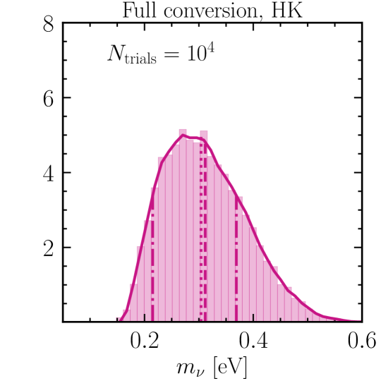
Fixed a neutrino detector, a conversion scenario, and a distance to the SN, we draw the number of observed events from the hypothesis in the time window 1.225 - 1.233 s with 0.1 ms bins, and use Eqs. 15–16 to calculate the for . The neutrino mass, which corresponds to the critical value of the distribution for the 95% C.L. (equal to 3.81 for 1 degree of freedom (d.o.f)), is the calculated upper limit from a single trial. We repeat this procedure many times () to construct the probability density distribution of the limits from single trials (Fig. 9 in Appendix B). The median of the obtained distribution is the final 95% C.L. on the absolute neutrino mass. Since the distributions are not Gaussian (see Fig. 9 in Appendix B), we determine the 68% C.L. uncertainty on the median 95% C.L. upper limit via the Feldman-Cousins procedure to ensure consistent coverage Feldman and Cousins (1998). The lower and upper uncertainties on the 95% C.L. upper limit are the solutions to
| (17) |
where is the constructed probability density distribution and . The calculated 95% C.L. upper limits for a SN at a distance 10 kpc for all three considered detectors, and both oscillation scenarios are summarized in Table 2.
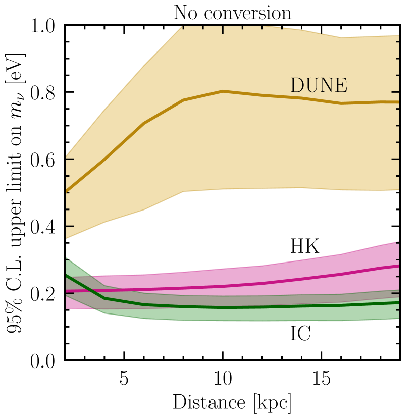
Figure 6 shows the 95%C.L. upper limits on the neutrino mass and their uncertainty from the HK (pink), IC (green), and DUNE (yellow) as a function of the distance to the SN for both considered neutrino conversion cases. These limits and their uncertainty range were calculated for to save the computational expenses. We have checked that increasing the number of trials does not affect the limits and their uncertainties more than approximately 2%. For example, in the the full conversion scenario from HK detector for and SN at a distance 10 kpc the median, mean, lower uncertainty, and upper uncertainty of the limit are 0.304, 0.312, 0.215, and 0.369, respectively (see the left panel of Fig. 10 in Appendix C), whereas for these numbers change to 0.305, 0.313, 0.215, and 0.373 (see the Table 2 and the lower right panel of the Fig. 9 in Appendix B).
The IC experiment results in the best limits on the neutrino mass from QHPT peak for SN at distances greater than approximately 5 kpc due to its largest volume and lowest energy threshold among the considered detectors. For SN occurring closer to the Earth, however, the HK detector yields better limits because the dead-time efficiency significantly reduces the neutrino signal in the IC during the QHPT peak. DUNE, owing to the smallest volume and lowest effective threshold, is expected to provide the weakest limits on the neutrino mass.
In addition, in the case of no conversion, the calculated limits are stronger in HK and IC than in the full conversion case, and the opposite is true for DUNE. This is due to the hierarchy of the luminosities and mean energies of the different neutrino flavors emitted from the SN (see Fig. 1). The mean energies and luminosities for are the lowest during the QHPT peak; therefore, the limits from DUNE in the no conversion case are worse than in full conversion. On the other hand, the mean energies of are larger than , but the luminosity of is larger than . Combining that with shorter time delays for more energetic neutrinos (Eq. 3) leads to better limits in the no conversion than full conversion case for IC and HK. The effect is, however, not as striking as for DUNE.
We have also checked that including a normalization uncertainty in the likelihood calculation and marginalizing over it does not affect our results significantly. This is because the nonzero neutrino masses reduce the left side of the QHPT neutrino peak while extending the right slope, effectively widening and flattening the peak, an effect that cannot be mimicked by changing the normalization.
VI Discussion and Conclusions
Core-collapse supernovae are one of the most complex phenomena in the universe. Not only are they a site of production of the heavy elements which enable the existence of life, but their cores are also one of the densest environments we can indirectly probe. At such densities, the matter may no longer consist only of hadronic degrees of freedom but undergo a phase transition to quark matter. It has been shown that such transition can cause a prominent burst of in the early postbounce phase after the neutronization burst release. The detection of such a sharp feature in the neutrino signal from a core-collapse supernova at the Earth would not only strongly back the existence of the quark-hadron phase transition, but also allow us to set stringent limits on the neutrino masses and help to identify the supernova location by the triangulation technique.
In this work, we show that triangulating supernova using the quark-hadron phase transition peak can significantly improve the pointing precision of the supernova localization within the galactic neighborhood compared to using the neutronization peak. Given the characteristic flavor composition, energy dependence of the sharp burst, and considered detectors, the case with full conversion between the neutrino flavors leads to the best determination of the collapsing star’s location, i.e., angular uncertainty for a supernova at distance of 10 kpc. In the case of no conversion between the flavors the pointing precising reduces to .
Our method leads up to times improvement in comparison to utilizing the neutronization burst Beacom and Vogel (1999); Mühlbeier et al. (2013); Brdar et al. (2018); Hansen et al. (2020); Linzer and Scholberg (2019); Coleiro et al. (2020) to triangulate supernova, while comparable results have been found by using the endpoint of the neutrino signal for progenitors directly forming black holes Mühlbeier et al. (2013); Brdar et al. (2018); Hansen et al. (2020); Sarfati et al. (2022). Even though better techniques to pinpoint the SN location exist, i.e., using the directionality of interaction channels such as neutrino elastic scattering off electrons, an optimal approach is to gather all the available information by exploiting all existing methods and complementary strategies.
We also show that observation of the sharp burst associated with the quark-hadron phase transition can set competitive limits on the neutrino mass. We find that IC can reach the 95% C.L. sensitivity of 0.16 eV, HK 0.22 eV, and DUNE 0.58 eV for supernova at a distance 10 kpc from the Earth for favorable conversion scenarios, i.e., no conversions for HK and IC, and full flavor swap for DUNE. The limits for the opposite conversion scenarios are 0.21 eV, 0.30 eV, and 0.80 eV for IC, HK, and DUNE, respectively. The calculated upper limits on the neutrino mass are more stringent than the ones from the laboratory experiments 0.8 eV Aker et al. (2022) and the limits obtained from the supernova neutronization burst analyses Nardi and Zuluaga (2004, 2005); Pagliaroli et al. (2010); Lu et al. (2015); Rossi-Torres et al. (2015); Hansen et al. (2020); Pompa et al. (2022). In addition, they are comparable to the bounds found using the end time of the neutrino signal from a black-hole-forming core-collapse supernova in cases with low accretion Beacom et al. (2000); Hansen et al. (2020). We expect that detectors with comparable characteristics that encompass energy thresholds, time resolutions and effective volumes such as, e.g., SK or JUNO, can yield similar results to the ones found in our paper.
The existence of the hadron-quark phase transition in the core-collapse supernova may not only be imprinted in the neutrino signal, but also gravitational waves Blacker et al. (2020). In such a case, the time difference between the gravitational wave and neutrino signals may also be used to ascertain the neutrino mass limits, as in the neutronization burst and BH formation cases Pagliaroli et al. (2009); Hansen et al. (2020). Moreover, the quark-hadron phase transition can result in increased entropy and neutron richness in the neutrino-driven wind Fischer et al. (2020), setting an optimal condition for the process.
In our work, we rely on a specific model of the core-collapse supernova with a burst released by the quark-hadron phase transition. The results presented here, however, should not change significantly for different models because the heights and widths of the peak are comparable in those, see e.g., Refs. Dasgupta et al. (2010); Jakobus et al. (2022). Nevertheless, it would be interesting to see a study focused on how the theoretical uncertainties inherent in the modeling of the phase transition in the supernova affect the emitted neutrino spectra.
Acknowledgements.
We are grateful for helpful discussions with George Fuller, Massimiliano Lincetto, Shashank Shalgar, Toshio Suzuki, Mark Vagins, Anna Watts, and especially Peter Denton, Rasmus Hansen, and Kate Scholberg. We also thank Tobias Fischer for useful insights and access to the supernova-models. T.P would like to thank Irene Tamborra for the support during the course of this project. This work was supported in part by the National Science Foundation Grants No. PHY-2020275 and PHY-2108339. T.P acknowledges support from the Carlsberg Foundation (CF18-0183). A.M.S. and A.B.B would like to thank Kavli Institute for Theoretical Physics (KITP) for the hospitality during this work. KITP issupported in part by the National Science Foundation under Grant No. NSF PHY-1748958. We acknowledge the use of the matplotlib Hunter (2007) and Astropy python packages Astropy Collaboration et al. (2013, 2018).Appendix A Histograms: timing the neutrino signal
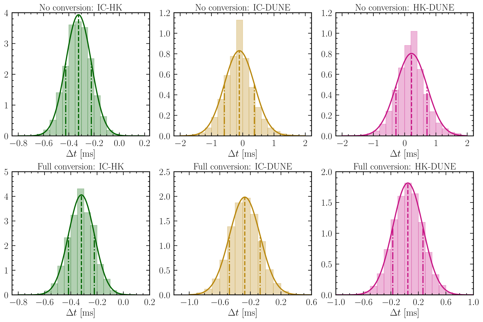
We show the constructed distribution of the biases between the pairs of the considered detectors for the QHPT neutrino burst time determination in Fig. 7 for a SN at a distance of 10 kpc. In all of the displayed cases, the calculated distribution are well fitted with the Gaussians (solid lines) characterized by the mean (dashed lines) and standard deviation (dash-dotted lines) from .
Additionally, in Fig. 8 we show how the determination of the SN localization on the sky weakens in case the distance to the Earth increases to 20 kpc.
Appendix B Histograms: neutrino mass limit
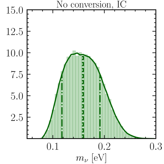

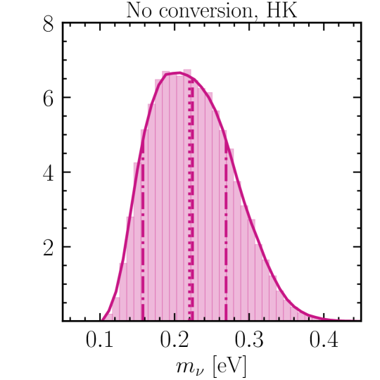
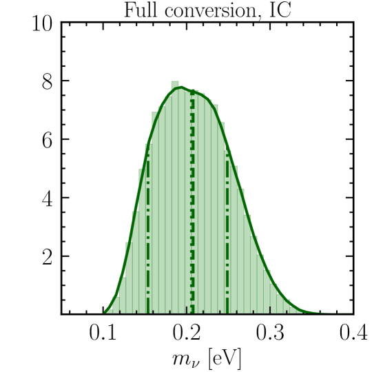
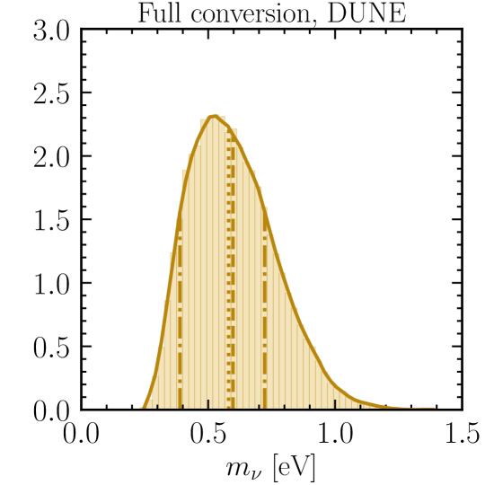
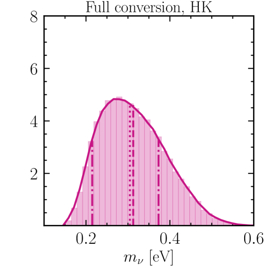
Fig. 9 shows the probability density distributions of the upper limits on the absolute neutrino mass calculated using the QHPT peak in the neutrino signal from a SN at a distance 10 kpc from the Earth from IC (left panels; green), DUNE (middle panels; yellow), and HK (right panels; pink) in the no conversion (upper panels) and full conversion oscillation scenarios for . Although the means (dashed lines) and medians (dotted lines) for each distribution do not differ significantly the skewed high mass tail causes the distribution to diverge from the normal distribution and produces an asymmetric uncertainty band for the calculated mass limits.
Appendix C Changes of the critical value for low neutrino mass
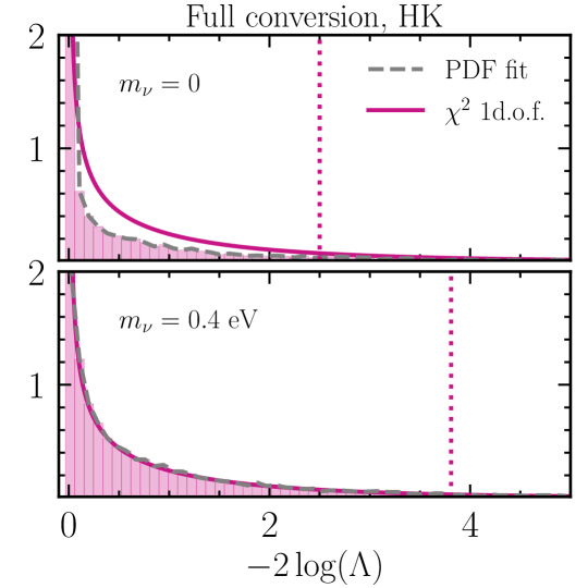
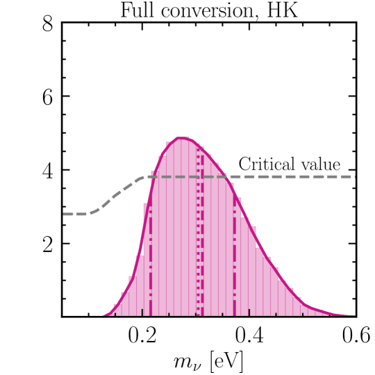
The critical value for the hypotheses tested using the likelihood method is often times approximated by the critical value for the distribution with the number of d.o.f. corresponding to the number of free parameters of the model, i.e., Wilks’ theorem Wilks (1938). We have checked that using the Wilks’ theorem approximation is valid for sufficiently high masses, whereas for small ones, the critical value obtained from using the Feldman-Cousins prescription Feldman and Cousins (1998) is smaller. The middle panel illustrates the above on the HK ”Full conversion” example. Assuming the eV hypothesis being true, we draw event rates and calculate the likelihood distribution. It turns out that it closely follow the distribution with 1 d.o.f. hence, the critical value of that particular mass is also well approximated by the critical value distribution with 1 d.o.f. This is, however, not true for . Due to this effect, the critical value for low masses is reduced. The limits obtained using the true critical value (gray dashed line in right panel of Fig. 10), however, change only slightly, as can be seen in the right panel of Fig. 10. The main difference with respect to distributions calculated assuming Wilks’ theorem is a more extended left side tail of the distribution leading to slightly lower limit on the neutrino mass. The used approach, Wilks’ theorem approximation, therefore, does not make the limits calculated in our work significantly discrepant from the ones obtained by relaxing that assumption.
References
- Hirata et al. (1987) K. Hirata, T. Kajita, M. Koshiba, M. Nakahata, Y. Oyama, N. Sato, A. Suzuki, M. Takita, Y. Totsuka, T. Kifune, T. Suda, K. Takahashi, T. Tanimori, K. Miyano, M. Yamada, E. W. Beier, L. R. Feldscher, S. B. Kim, A. K. Mann, F. M. Newcomer, R. Van, W. Zhang, and B. G. Cortez, “Observation of a neutrino burst from the supernova sn1987a,” Phys. Rev. Lett. 58, 1490–1493 (1987).
- Bionta et al. (1987) R. M. Bionta et al., “Observation of a Neutrino Burst in Coincidence with Supernova SN 1987a in the Large Magellanic Cloud,” Phys. Rev. Lett. 58, 1494 (1987).
- Alexeyev et al. (1988) E.N. Alexeyev, L.N. Alexeyeva, I.V. Krivosheina, and V.I. Volchenko, “Detection of the neutrino signal from sn 1987a in the lmc using the inr baksan underground scintillation telescope,” Physics Letters B 205, 209–214 (1988).
- Janka (2017) H. Th. Janka, “Neutrino Emission from Supernovae,” (2017), 10.1007/978-3-319-21846-5_4, arXiv:1702.08713 [astro-ph.HE] .
- Burrows and Vartanyan (2021) Adam Burrows and David Vartanyan, “Core-Collapse Supernova Explosion Theory,” Nature 589, 29–39 (2021), arXiv:2009.14157 [astro-ph.SR] .
- Brown et al. (1982) G. E. Brown, H. A. Bethe, and Gordon Baym, “Supernova theory,” Nucl. Phys. A 375, 481–532 (1982).
- Bethe et al. (1979) H. A. Bethe, G. E. Brown, J. Applegate, and J. M. Lattimer, “Equation of state in the gravitational collapse of stars,” Nucl. Phys. A 324, 487–533 (1979).
- Fuller et al. (1982) George M. Fuller, William A. Fowler, and Michael J. Newman, “Stellar Weak Interaction Rates for Intermediate Mass Nuclei. 2. A = 21 to A = 60,” Astrophys. J. 252, 715–740 (1982).
- Mirizzi et al. (2016) Alessandro Mirizzi, Irene Tamborra, Hans-Thomas Janka, Ninetta Saviano, Kate Scholberg, Robert Bollig, Lorenz Hudepohl, and Sovan Chakraborty, “Supernova Neutrinos: Production, Oscillations and Detection,” Riv. Nuovo Cim. 39, 1–112 (2016), arXiv:1508.00785 [astro-ph.HE] .
- Horiuchi and Kneller (2018) Shunsaku Horiuchi and James P Kneller, “What can be learned from a future supernova neutrino detection?” J. Phys. G 45, 043002 (2018), arXiv:1709.01515 [astro-ph.HE] .
- Colgate and White (1966) Stirling A. Colgate and Richard H. White, “The Hydrodynamic Behavior of Supernovae Explosions,” Astrophys. J. 143, 626 (1966).
- Bethe and Wilson (1985) Hans A. Bethe and James R. Wilson, “Revival of a stalled supernova shock by neutrino heating,” Astrophys. J. 295, 14–23 (1985).
- Raffelt (2001) Georg G. Raffelt, “Muon-neutrino and tau-neutrino spectra formation in supernovae,” Astrophys. J. 561, 890–914 (2001), arXiv:astro-ph/0105250 .
- Fischer et al. (2012) T. Fischer, G. Martinez-Pinedo, M. Hempel, and M. Liebendorfer, “Neutrino spectra evolution during proto-neutron star deleptonization,” Phys. Rev. D 85, 083003 (2012), arXiv:1112.3842 [astro-ph.HE] .
- Blondin et al. (2003) John M. Blondin, Anthony Mezzacappa, and Christine DeMarino, “Stability of standing accretion shocks, with an eye toward core collapse supernovae,” Astrophys. J. 584, 971–980 (2003), arXiv:astro-ph/0210634 .
- Tamborra et al. (2014) Irene Tamborra, Florian Hanke, Hans-Thomas Janka, Bernhard Müller, Georg G. Raffelt, and Andreas Marek, “Self-sustained asymmetry of lepton-number emission: A new phenomenon during the supernova shock-accretion phase in three dimensions,” Astrophys. J. 792, 96 (2014), arXiv:1402.5418 [astro-ph.SR] .
- Couch and Ott (2015) Sean M. Couch and Christian D. Ott, “The Role of Turbulence in Neutrino-Driven Core-Collapse Supernova Explosions,” Astrophys. J. 799, 5 (2015), arXiv:1408.1399 [astro-ph.HE] .
- Abdikamalov et al. (2015) Ernazar Abdikamalov, Christian D. Ott, David Radice, Luke F. Roberts, Roland Haas, Christian Reisswig, Philipp Mösta, Hannah Klion, and Erik Schnetter, “Neutrino-driven Turbulent Convection and Standing Accretion Shock Instability in Three-Dimensional Core-Collapse Supernovae,” Astrophys. J. 808, 70 (2015), arXiv:1409.7078 [astro-ph.HE] .
- Galama et al. (1998) T. J. Galama et al., “Discovery of the peculiar supernova 1998bw in the error box of GRB 980425,” Nature 395, 670 (1998), arXiv:astro-ph/9806175 .
- Stanek et al. (2003) Krzysztof Z. Stanek et al., “Spectroscopic discovery of the supernova 2003dh associated with GRB 030329,” Astrophys. J. Lett. 591, L17–L20 (2003), arXiv:astro-ph/0304173 .
- Hjorth et al. (2003) Jens Hjorth et al., “A Very energetic supernova associated with the gamma-ray burst of 29 March 2003,” Nature 423, 847–850 (2003), arXiv:astro-ph/0306347 .
- Della Valle et al. (2006) M. Della Valle et al., “Hypernova signatures in the late rebrightening of grb 050525a,” Astrophys. J. Lett. 642, L103–L106 (2006), arXiv:astro-ph/0604109 .
- LeBlanc and Wilson (1970) J. M. LeBlanc and J. R. Wilson, “A Numerical Example of the Collapse of a Rotating Magnetized Star,” Astrophys. J. 161, 541 (1970).
- Takiwaki et al. (2009) Tomoya Takiwaki, Kei Kotake, and Katsuhiko Sato, “Special Relativistic Simulations of Magnetically-dominated Jets in Collapsing Massive Stars,” Astrophys. J. 691, 1360–1379 (2009), arXiv:0712.1949 [astro-ph] .
- Mösta et al. (2015) Philipp Mösta, Christian D. Ott, David Radice, Luke F. Roberts, Erik Schnetter, and Roland Haas, “A large scale dynamo and magnetoturbulence in rapidly rotating core-collapse supernovae,” Nature 528, 376 (2015), arXiv:1512.00838 [astro-ph.HE] .
- Obergaulinger and Aloy (2021) Martin Obergaulinger and Miguel-Ángel Aloy, “Magnetorotational core collapse of possible GRB progenitors. III. Three-dimensional models,” Mon. Not. Roy. Astron. Soc. 503, 4942–4963 (2021), arXiv:2008.07205 [astro-ph.HE] .
- Matsumoto et al. (2022) Jin Matsumoto, Yuta Asahina, Tomoya Takiwaki, Kei Kotake, and Hiroyuki R. Takahashi, “Magnetic support for neutrino-driven explosion of 3D non-rotating core-collapse supernova models,” Mon. Not. Roy. Astron. Soc. 516, 1752–1767 (2022), arXiv:2202.07967 [astro-ph.HE] .
- Burrows et al. (2006) Adam Burrows, Eli Livne, Luc Dessart, Christian Ott, and Jeremiah Murphy, “A new mechanism for core-collapse supernova explosions,” Astrophys. J. 640, 878–890 (2006), arXiv:astro-ph/0510687 .
- Gossan et al. (2020) Sarah E. Gossan, Jim Fuller, and Luke F. Roberts, “Wave heating from proto-neutron star convection and the core-collapse supernova explosion mechanism,” Mon. Not. Roy. Astron. Soc. 491, 5376–5391 (2020), arXiv:1910.07599 [astro-ph.HE] .
- Fuller et al. (2009) George M. Fuller, Alexander Kusenko, and Kalliopi Petraki, “Heavy sterile neutrinos and supernova explosions,” Phys. Lett. B 670, 281–284 (2009), arXiv:0806.4273 [astro-ph] .
- Rembiasz et al. (2018) Tomasz Rembiasz, Martin Obergaulinger, Manuel Masip, M. Ángeles Pérez-García, Miguel-Ángel Aloy, and Conrado Albertus, “Heavy sterile neutrinos in stellar core-collapse,” Phys. Rev. D 98, 103010 (2018), arXiv:1806.03300 [astro-ph.HE] .
- Mastrototaro et al. (2020) Leonardo Mastrototaro, Alessandro Mirizzi, Pasquale Dario Serpico, and Arman Esmaili, “Heavy sterile neutrino emission in core-collapse supernovae: Constraints and signatures,” JCAP 01, 010 (2020), arXiv:1910.10249 [hep-ph] .
- Qian et al. (1993) Yong-Zhong Qian, George M. Fuller, Grant J. Mathews, Ron Mayle, James R. Wilson, and S. E. Woosley, “A Connection between flavor mixing of cosmologically significant neutrinos and heavy element nucleosynthesis in supernovae,” Phys. Rev. Lett. 71, 1965–1968 (1993).
- Sigl (1995) G. Sigl, “Neutrino mixing constraints and supernova nucleosynthesis,” Phys. Rev. D 51, 4035–4044 (1995), arXiv:astro-ph/9410094 .
- Hidaka and Fuller (2006) Jun Hidaka and George M. Fuller, “Dark matter sterile neutrinos in stellar collapse: Alteration of energy/lepton number transport and a mechanism for supernova explosion enhancement,” Phys. Rev. D 74, 125015 (2006), arXiv:astro-ph/0609425 .
- Suliga et al. (2020) Anna M. Suliga, Irene Tamborra, and Meng-Ru Wu, “Lifting the core-collapse supernova bounds on keV-mass sterile neutrinos,” JCAP 08, 018 (2020), arXiv:2004.11389 [astro-ph.HE] .
- Sagert et al. (2009) I. Sagert, T. Fischer, M. Hempel, G. Pagliara, J. Schaffner-Bielich, A. Mezzacappa, F. K. Thielemann, and M. Liebendorfer, “Signals of the QCD phase transition in core-collapse supernovae,” Phys. Rev. Lett. 102, 081101 (2009), arXiv:0809.4225 [astro-ph] .
- Fischer et al. (2011) T. Fischer, I. Sagert, G. Pagliara, M. Hempel, J. Schaffner-Bielich, T. Rauscher, F. K. Thielemann, R. Kappeli, G. Martinez-Pinedo, and M. Liebendorfer, “Core-collapse supernova explosions triggered by a quark-hadron phase transition during the early post-bounce phase,” Astrophys. J. Suppl. 194, 39 (2011), arXiv:1011.3409 [astro-ph.HE] .
- Fischer et al. (2018) Tobias Fischer, Niels-Uwe F. Bastian, Meng-Ru Wu, Petr Baklanov, Elena Sorokina, Sergei Blinnikov, Stefan Typel, Thomas Klähn, and David B. Blaschke, “Quark deconfinement as a supernova explosion engine for massive blue supergiant stars,” Nature Astron. 2, 980–986 (2018), arXiv:1712.08788 [astro-ph.HE] .
- Zha et al. (2021) Shuai Zha, Evan P. O’Connor, and André da Silva Schneider, “Progenitor Dependence of Hadron-quark Phase Transition in Failing Core-collapse Supernovae,” Astrophys. J. 911, 74 (2021), arXiv:2103.02268 [astro-ph.HE] .
- Fischer (2021) Tobias Fischer, “QCD phase transition drives supernova explosion of a very massive star: Dependence on metallicity of the progenitor star,” Eur. Phys. J. A 57, 270 (2021), arXiv:2108.00196 [astro-ph.HE] .
- Kuroda et al. (2022) Takami Kuroda, Tobias Fischer, Tomoya Takiwaki, and Kei Kotake, “Core-collapse Supernova Simulations and the Formation of Neutron Stars, Hybrid Stars, and Black Holes,” Astrophys. J. 924, 38 (2022), arXiv:2109.01508 [astro-ph.HE] .
- Bauswein et al. (2022) Andreas Bauswein, David Blaschke, and Tobias Fischer, “Effects of a strong phase transition on supernova explosions, compact stars and their mergers,” (2022) arXiv:2203.17188 [nucl-th] .
- Lin et al. (2022) Zidu Lin, Shuai Zha, Evan P. O’Connor, and Andrew W. Steiner, “Detectability of hadron-quark phase transition in neutrino signals of failing core-collapse supernova,” (2022), arXiv:2203.05141 [astro-ph.HE] .
- Jakobus et al. (2022) Pia Jakobus, Bernhard Mueller, Alexander Heger, Anton Motornenko, Jan Steinheimer, and Horst Stoecker, “The Role of the Hadron-Quark Phase Transition in Core-Collapse Supernovae,” (2022), 10.1093/mnras/stac2352, arXiv:2204.10397 [astro-ph.HE] .
- Halzen and Raffelt (2009) Francis Halzen and Georg G. Raffelt, “Reconstructing the supernova bounce time with neutrinos in IceCube,” Phys. Rev. D 80, 087301 (2009), arXiv:0908.2317 [astro-ph.HE] .
- Abe et al. (2018) K. Abe et al. (Hyper-Kamiokande), “Hyper-Kamiokande Design Report,” (2018), arXiv:1805.04163 [physics.ins-det] .
- Abi et. al. (2020) Babak Abi et. al. (DUNE), “Deep Underground Neutrino Experiment (DUNE), Far Detector Technical Design Report, Volume II: DUNE Physics,” (2020), arXiv:2002.03005 [hep-ex] .
- Dasgupta et al. (2010) Basudeb Dasgupta, Tobias Fischer, Shunsaku Horiuchi, Matthias Liebendorfer, Alessandro Mirizzi, Irina Sagert, and Jurgen Schaffner-Bielich, “Detecting the QCD phase transition in the next Galactic supernova neutrino burst,” Phys. Rev. D 81, 103005 (2010), arXiv:0912.2568 [astro-ph.HE] .
- Bethe (1990) H. A. Bethe, “Supernova mechanisms,” Rev. Mod. Phys. 62, 801–866 (1990).
- Woosley et al. (2002) S. E. Woosley, A. Heger, and T. A. Weaver, “The evolution and explosion of massive stars,” Rev. Mod. Phys. 74, 1015–1071 (2002).
- Gerlach (1968) Ulrich H. Gerlach, “Equation of State at Supranuclear Densities and the Existence of a Third Family of Superdense Stars,” Phys. Rev. 172, 1325–1330 (1968).
- Alford et al. (2013) Mark G. Alford, Sophia Han, and Madappa Prakash, “Generic conditions for stable hybrid stars,” Phys. Rev. D 88, 083013 (2013), arXiv:1302.4732 [astro-ph.SR] .
- Espino and Paschalidis (2022) Pedro L. Espino and Vasileios Paschalidis, “Fate of twin stars on the unstable branch: Implications for the formation of twin stars,” Phys. Rev. D 105, 043014 (2022), arXiv:2105.05269 [astro-ph.HE] .
- Migdal et al. (1979) Arkady B. Migdal, A. I. Chernoutsan, and I. N. Mishustin, “PION CONDENSATION AND DYNAMICS OF NEUTRON STARS,” Phys. Lett. B 83, 158–160 (1979).
- Takahara and Sato (1988) M. Takahara and K. Sato, “Phase Transitions in the Newly Born Neutron Star and Neutrino Emissions From SN1987A,” Prog. Theor. Phys. 80, 861–867 (1988).
- Gentile et al. (1993) N. A. Gentile, M. B. Aufderheide, G. J. Mathews, F. D. Swesty, and G. M. Fuller, “The QCD phase transition and supernova core collapse,” Astrophys. J. 414, 701–711 (1993).
- Pons et al. (2001) Jose A. Pons, Andrew W. Steiner, Madappa Prakash, and James M. Lattimer, “Evolution of protoneutron stars with quarks,” Phys. Rev. Lett. 86, 5223–5226 (2001), arXiv:astro-ph/0102015 .
- Drago et al. (2008) Alessandro Drago, Giuseppe Pagliara, Giulia Pagliaroli, Francesco Lorenzo Villante, and Francesco Vissani, “Formation of quark phases in compact stars and SN explosion,” AIP Conf. Proc. 1056, 256–263 (2008), arXiv:0809.0518 [astro-ph] .
- Nakazato et al. (2008) Ken’ichiro Nakazato, Kohsuke Sumiyoshi, and Shoichi Yamada, “Astrophysical Implications of Equation of State for Hadron-Quark Mixed Phase: Compact Stars and Stellar Collapses,” Phys. Rev. D 77, 103006 (2008), arXiv:0804.0661 [astro-ph] .
- Liebendoerfer et al. (2004) M. Liebendoerfer, O. E. B. Messer, A. Mezzacappa, S. W. Bruenn, C. Y. Cardall, and F. K. Thielemann, “A Finite difference representation of neutrino radiation hydrodynamics for spherically symmetric general relativistic supernova simulations,” Astrophys. J. Suppl. 150, 263–316 (2004), arXiv:astro-ph/0207036 .
- Mezzacappa and Bruenn (1993) A. Mezzacappa and S. W. Bruenn, “A numerical method for solving the neutrino Boltzmann equation coupled to spherically symmetric stellar core collapse,” Astrophys. J. 405, 669–684 (1993).
- Bastian (2021) Niels-Uwe F. Bastian, “Phenomenological quark-hadron equations of state with first-order phase transitions for astrophysical applications,” Phys. Rev. D 103, 023001 (2021), arXiv:2009.10846 [nucl-th] .
- Kaltenborn et al. (2017) Mark Alexander Randolph Kaltenborn, Niels-Uwe Friedrich Bastian, and David Bernhard Blaschke, “Quark-nuclear hybrid star equation of state with excluded volume effects,” Phys. Rev. D 96, 056024 (2017), arXiv:1701.04400 [astro-ph.HE] .
- Riley et al. (2021) Thomas E. Riley et al., “A NICER View of the Massive Pulsar PSR J0740+6620 Informed by Radio Timing and XMM-Newton Spectroscopy,” Astrophys. J. Lett. 918, L27 (2021), arXiv:2105.06980 [astro-ph.HE] .
- Raaijmakers et al. (2021) G. Raaijmakers, S. K. Greif, K. Hebeler, T. Hinderer, S. Nissanke, A. Schwenk, T. E. Riley, A. L. Watts, J. M. Lattimer, and W. C. G. Ho, “Constraints on the Dense Matter Equation of State and Neutron Star Properties from NICER’s Mass–Radius Estimate of PSR J0740+6620 and Multimessenger Observations,” Astrophys. J. Lett. 918, L29 (2021), arXiv:2105.06981 [astro-ph.HE] .
- Keil et al. (2003) Mathias Th. Keil, Georg G. Raffelt, and Hans-Thomas Janka, “Monte Carlo study of supernova neutrino spectra formation,” Astrophys. J. 590, 971–991 (2003), arXiv:astro-ph/0208035 .
- Keil (2003) Mathias Thorsten Keil, “Supernova neutrino spectra and applications to flavor oscillations, Master’s thesis,” (2003), arXiv:astro-ph/0308228 .
- Tamborra et al. (2012) Irene Tamborra, Bernhard Muller, Lorenz Hudepohl, Hans-Thomas Janka, and Georg Raffelt, “High-resolution supernova neutrino spectra represented by a simple fit,” Phys. Rev. D 86, 125031 (2012), arXiv:1211.3920 [astro-ph.SR] .
- Duan et al. (2010) Huaiyu Duan, George M. Fuller, and Yong-Zhong Qian, “Collective Neutrino Oscillations,” Ann. Rev. Nucl. Part. Sci. 60, 569–594 (2010), arXiv:1001.2799 [hep-ph] .
- Chakraborty et al. (2016) Sovan Chakraborty, Rasmus Hansen, Ignacio Izaguirre, and Georg Raffelt, “Collective neutrino flavor conversion: Recent developments,” Nucl. Phys. B 908, 366–381 (2016), arXiv:1602.02766 [hep-ph] .
- Tamborra and Shalgar (2020) Irene Tamborra and Shashank Shalgar, “New Developments in Flavor Evolution of a Dense Neutrino Gas,” (2020), 10.1146/annurev-nucl-102920-050505, arXiv:2011.01948 [astro-ph.HE] .
- Patwardhan et al. (2021) Amol V. Patwardhan, Michael J. Cervia, and A. B. Balantekin, “Spectral splits and entanglement entropy in collective neutrino oscillations,” Phys. Rev. D 104, 123035 (2021), arXiv:2109.08995 [hep-ph] .
- Wolfenstein (1978) L. Wolfenstein, “Neutrino Oscillations in Matter,” Phys. Rev. D 17, 2369–2374 (1978).
- Mikheev and Smirnov (1986) S. P. Mikheev and A. Yu. Smirnov, “Neutrino Oscillations in a Variable Density Medium and Neutrino Bursts Due to the Gravitational Collapse of Stars,” Sov. Phys. JETP 64, 4–7 (1986), [,311(1986)], arXiv:0706.0454 [hep-ph] .
- Nakamura et al. (2016) Ko Nakamura, Shunsaku Horiuchi, Masaomi Tanaka, Kazuhiro Hayama, Tomoya Takiwaki, and Kei Kotake, “Multimessenger signals of long-term core-collapse supernova simulations: synergetic observation strategies,” Mon. Not. Roy. Astron. Soc. 461, 3296–3313 (2016), arXiv:1602.03028 [astro-ph.HE] .
- Antonioli et al. (2004) Pietro Antonioli et al., “SNEWS: The Supernova Early Warning System,” New J. Phys. 6, 114 (2004), arXiv:astro-ph/0406214 .
- Pagliaroli et al. (2009) G. Pagliaroli, F. Vissani, E. Coccia, and W. Fulgione, “Neutrinos from Supernovae as a Trigger for Gravitational Wave Search,” Phys. Rev. Lett. 103, 031102 (2009), arXiv:0903.1191 [hep-ph] .
- Warren et al. (2020) MacKenzie L. Warren, Sean M. Couch, Evan P. O’Connor, and Viktoriya Morozova, “Constraining Properties of the Next Nearby Core-collapse Supernova with Multimessenger Signals,” Astrophys. J. 898, 139 (2020), arXiv:1912.03328 [astro-ph.HE] .
- Pajkos et al. (2021) Michael A. Pajkos, MacKenzie L. Warren, Sean M. Couch, Evan P. O’Connor, and Kuo-Chuan Pan, “Determining the Structure of Rotating Massive Stellar Cores with Gravitational Waves,” Astrophys. J. 914, 80 (2021), arXiv:2011.09000 [astro-ph.HE] .
- Halim et al. (2021) Odysse Halim, Claudio Casentini, Marco Drago, Viviana Fafone, Kate Scholberg, Carlo Francesco Vigorito, and Giulia Pagliaroli, “Multimessenger analysis strategy for core-collapse supernova search: gravitational waves and low-energy neutrinos,” JCAP 11, 021 (2021), arXiv:2107.02050 [astro-ph.HE] .
- Beacom and Vogel (1999) John F. Beacom and P. Vogel, “Can a supernova be located by its neutrinos?” Phys. Rev. D 60, 033007 (1999), arXiv:astro-ph/9811350 .
- Tomas et al. (2003) R. Tomas, D. Semikoz, G. G. Raffelt, M. Kachelriess, and A. S. Dighe, “Supernova pointing with low-energy and high-energy neutrino detectors,” Phys. Rev. D 68, 093013 (2003), arXiv:hep-ph/0307050 .
- Mühlbeier et al. (2013) T. Mühlbeier, H. Nunokawa, and R. Zukanovich Funchal, “Revisiting the Triangulation Method for Pointing to Supernova and Failed Supernova with Neutrinos,” Phys. Rev. D 88, 085010 (2013), arXiv:1304.5006 [astro-ph.HE] .
- Brdar et al. (2018) Vedran Brdar, Manfred Lindner, and Xun-Jie Xu, “Neutrino astronomy with supernova neutrinos,” JCAP 04, 025 (2018), arXiv:1802.02577 [hep-ph] .
- Hansen et al. (2020) Rasmus S. L. Hansen, Manfred Lindner, and Oliver Scholer, “Timing the neutrino signal of a Galactic supernova,” Phys. Rev. D 101, 123018 (2020), arXiv:1904.11461 [hep-ph] .
- Linzer and Scholberg (2019) N. B. Linzer and K. Scholberg, “Triangulation pointing to core-collapse supernovae with next-generation neutrino detectors,” Phys. Rev. D 100, 103005 (2019).
- Coleiro et al. (2020) A. Coleiro, M. Colomer Molla, D. Dornic, M. Lincetto, and V. Kulikovskiy, “Combining neutrino experimental light-curves for pointing to the next galactic core-collapse supernova,” Eur. Phys. J. C 80, 856 (2020), arXiv:2003.04864 [astro-ph.HE] .
- Sarfati et al. (2022) Lila Sarfati, Rasmus S. L. Hansen, and Irene Tamborra, “Triangulating black hole forming stellar collapses through neutrinos,” Phys. Rev. D 105, 023011 (2022).
- Scholberg et al. (2010) Kate Scholberg, Armin Burgmeier, and Roger Wendell, “Obtaining supernova directional information using the neutrino matter oscillation pattern,” Phys. Rev. D 81, 043007 (2010), arXiv:0910.3174 [astro-ph.IM] .
- Ertl et al. (2016) T. Ertl, H.-Th. Janka, S. E. Woosley, T. Sukhbold, and M. Ugliano, “A two-parameter criterion for classifying the explodability of massive stars byb the neutrino-driven mechanism,” The Astrophysical Journal 818, 124 (2016).
- Couch et al. (2020) Sean M. Couch, MacKenzie L. Warren, and Evan P. O’Connor, “Simulating turbulence-aided neutrino-driven core-collapse supernova explosions in one dimension,” The Astrophysical Journal 890, 127 (2020).
- Sukhbold et al. (2016) Tuguldur Sukhbold, T. Ertl, S. E. Woosley, Justin M. Brown, and H.-T. Janka, “Core-collapse supernovae from 9 to 12 solar masses based on neutrino-powered explosions,” The Astrophysical Journal 821, 38 (2016).
- Adams et al. (2017a) S. M. Adams, C. S. Kochanek, J. R. Gerke, K. Z. Stanek, and X. Dai, “The search for failed supernovae with the Large Binocular Telescope: confirmation of a disappearing star,” Monthly Notices of the Royal Astronomical Society 468, 4968–4981 (2017a), https://academic.oup.com/mnras/article-pdf/468/4/4968/16638468/stx816.pdf .
- Adams et al. (2017b) S. M. Adams, C. S. Kochanek, J. R. Gerke, and K. Z. Stanek, “The search for failed supernovae with the Large Binocular Telescope: constraints from 7 yr of data,” Monthly Notices of the Royal Astronomical Society 469, 1445–1455 (2017b), https://academic.oup.com/mnras/article-pdf/469/2/1445/17272527/stx898.pdf .
- Neustadt et al. (2021) J M M Neustadt, C S Kochanek, K Z Stanek, C Basinger, T Jayasinghe, C T Garling, S M Adams, and J Gerke, “The search for failed supernovae with the Large Binocular Telescope: a new candidate and the failed SN fraction with 11 yr of data,” Monthly Notices of the Royal Astronomical Society 508, 516–528 (2021), https://academic.oup.com/mnras/article-pdf/508/1/516/40440715/stab2605.pdf .
- Wang et al. (2021) Jia-Shian Wang, Jeff Tseng, Samuel Gullin, and Evan P. O’Connor, “Nonradial neutrino emission upon black hole formation in core collapse supernovae,” Phys. Rev. D 104, 104030 (2021), arXiv:2109.11430 [astro-ph.HE] .
- Fukuda et al. (1998) Y. Fukuda et al. (Super-Kamiokande), “Evidence for oscillation of atmospheric neutrinos,” Phys. Rev. Lett. 81, 1562–1567 (1998), arXiv:hep-ex/9807003 .
- Hirata et al. (1992) K. S. Hirata et al. (Kamiokande-II), “Observation of a small atmospheric muon-neutrino / electron-neutrino ratio in Kamiokande,” Phys. Lett. B 280, 146–152 (1992).
- Bellerive et al. (2016) A. Bellerive, J. R. Klein, A. B. McDonald, A. J. Noble, and A. W. P. Poon (SNO), “The Sudbury Neutrino Observatory,” Nucl. Phys. B 908, 30–51 (2016), arXiv:1602.02469 [nucl-ex] .
- Zyla et al. (2020) P.A. Zyla et al. (Particle Data Group), “Review of Particle Physics,” PTEP 2020, 083C01 (2020).
- Gariazzo et al. (2018) S. Gariazzo, M. Archidiacono, P. F. de Salas, O. Mena, C. A. Ternes, and M. Tórtola, “Neutrino masses and their ordering: Global Data, Priors and Models,” JCAP 03, 011 (2018), arXiv:1801.04946 [hep-ph] .
- Jimenez et al. (2022) Raul Jimenez, Carlos Pena-Garay, Kathleen Short, Fergus Simpson, and Licia Verde, “Neutrino Masses and Mass Hierarchy: Evidence for the Normal Hierarchy,” (2022), arXiv:2203.14247 [hep-ph] .
- Chudaykin et al. (2022) Anton Chudaykin, Dmitry Gorbunov, and Nikita Nedelko, “Exploring CDM extensions with SPT-3G and Planck data: 4 evidence for neutrino masses, full resolution of the Hubble crisis by dark energy with phantom crossing, and all that,” (2022), arXiv:2203.03666 [astro-ph.CO] .
- Gariazzo et al. (2022) Stefano Gariazzo et al., “Neutrino mass and mass ordering: No conclusive evidence for normal ordering,” (2022), arXiv:2205.02195 [hep-ph] .
- Angrik et al. (2005) J. Angrik et al. (KATRIN), “KATRIN design report 2004,” (2005).
- Aker et al. (2022) M. Aker et al. (KATRIN), “Direct neutrino-mass measurement with sub-electronvolt sensitivity,” Nature Phys. 18, 160–166 (2022), arXiv:2105.08533 [hep-ex] .
- Zatsepin (1968) G. T. Zatsepin, “On the possibility of determining the upper limit of the neutrino mass by means of the flight time,” Pisma Zh. Eksp. Teor. Fiz. 8, 333–334 (1968).
- Loredo and Lamb (2002) Thomas J. Loredo and Don Q. Lamb, “Bayesian analysis of neutrinos observed from supernova SN-1987A,” Phys. Rev. D 65, 063002 (2002), arXiv:astro-ph/0107260 .
- Pagliaroli et al. (2010) G. Pagliaroli, F. Rossi-Torres, and F. Vissani, “Neutrino mass bound in the standard scenario for supernova electronic antineutrino emission,” Astropart. Phys. 33, 287–291 (2010), arXiv:1002.3349 [hep-ph] .
- Nardi and Zuluaga (2004) Enrico Nardi and Jorge I. Zuluaga, “Exploring the sub-eV neutrino mass range with supernova neutrinos,” Phys. Rev. D 69, 103002 (2004), arXiv:astro-ph/0306384 .
- Nardi and Zuluaga (2005) Enrico Nardi and Jorge I. Zuluaga, “Constraints on neutrino masses from a galactic supernova neutrino signal at present and future detectors,” Nucl. Phys. B 731, 140–163 (2005), arXiv:hep-ph/0412104 .
- Lu et al. (2015) Jia-Shu Lu, Jun Cao, Yu-Feng Li, and Shun Zhou, “Constraining Absolute Neutrino Masses via Detection of Galactic Supernova Neutrinos at JUNO,” JCAP 05, 044 (2015), arXiv:1412.7418 [hep-ph] .
- Rossi-Torres et al. (2015) F. Rossi-Torres, M. M. Guzzo, and E. Kemp, “Boundaries on Neutrino Mass from Supernovae Neutronization Burst by Liquid Argon Experiments,” (2015), arXiv:1501.00456 [hep-ph] .
- Pompa et al. (2022) Federica Pompa, Francesco Capozzi, Olga Mena, and Michel Sorel, “An absolute mass measurement with the DUNE experiment,” (2022), arXiv:2203.00024 [hep-ph] .
- Scholberg (2012) Kate Scholberg, “Supernova Neutrino Detection,” Ann. Rev. Nucl. Part. Sci. 62, 81–103 (2012), arXiv:1205.6003 [astro-ph.IM] .
- Al Kharusi et al. (2021) S. Al Kharusi et al. (SNEWS), “SNEWS 2.0: a next-generation supernova early warning system for multi-messenger astronomy,” New J. Phys. 23, 031201 (2021), arXiv:2011.00035 [astro-ph.HE] .
- Beacom et al. (2000) John F. Beacom, R. N. Boyd, and A. Mezzacappa, “Technique for direct eV scale measurements of the mu and tau neutrino masses using supernova neutrinos,” Phys. Rev. Lett. 85, 3568–3571 (2000), arXiv:hep-ph/0006015 .
- Gullin et al. (2022) Samuel Gullin, Evan P. O’Connor, Jia-Shian Wang, and Jeff Tseng, “Neutrino Echos following Black Hole Formation in Core-collapse Supernovae,” Astrophys. J. 926, 212 (2022), arXiv:2109.13242 [astro-ph.HE] .
- Serpico et al. (2012) Pasquale D. Serpico, Sovan Chakraborty, Tobias Fischer, Lorenz Hudepohl, Hans-Thomas Janka, and Alessandro Mirizzi, “Probing the neutrino mass hierarchy with the rise time of a supernova burst,” Phys. Rev. D 85, 085031 (2012), arXiv:1111.4483 [astro-ph.SR] .
- Brdar and Xu (2022) Vedran Brdar and Xun-Jie Xu, “Timing and multi-channel: novel method for determining the neutrino mass ordering from supernovae,” JCAP 08, 067 (2022), arXiv:2204.13135 [hep-ph] .
- Abbasi et al. (2011) R. Abbasi et al. (IceCube), “IceCube Sensitivity for Low-Energy Neutrinos from Nearby Supernovae,” Astron. Astrophys. 535, A109 (2011), [Erratum: Astron.Astrophys. 563, C1 (2014)], arXiv:1108.0171 [astro-ph.HE] .
- Abi et al. (2021) B. Abi et al. (DUNE), “Supernova neutrino burst detection with the Deep Underground Neutrino Experiment,” Eur. Phys. J. C 81, 423 (2021), arXiv:2008.06647 [hep-ex] .
- Strumia and Vissani (2003) Alessandro Strumia and Francesco Vissani, “Precise quasielastic neutrino/nucleon cross-section,” Phys. Lett. B 564, 42–54 (2003), arXiv:astro-ph/0302055 .
- Ricciardi et al. (2022) Giulia Ricciardi, Natascia Vignaroli, and Francesco Vissani, “An accurate evaluation of electron (anti-)neutrino scattering on nucleons,” JHEP 08, 212 (2022), arXiv:2206.05567 [hep-ph] .
- Halzen and Klein (2010) Francis Halzen and Spencer R. Klein, “IceCube: An Instrument for Neutrino Astronomy,” Rev. Sci. Instrum. 81, 081101 (2010), arXiv:1007.1247 [astro-ph.HE] .
- Freiherr Heereman von Zuydtwyck (2015) David Freiherr Heereman von Zuydtwyck, “HitSpooling: An Improvement for the Supernova Neutrino Detection System in IceCube, Ph.D. thesis,” (2015).
- Suzuki and Honma (2013) Toshio Suzuki and Michio Honma, “Neutrino Capture Reactions on 40Ar,” Phys. Rev. C 87, 014607 (2013), arXiv:1211.4078 [nucl-th] .
- Toshio Suzuki (2022) Toshio Suzuki, “private communication,” (2022).
- Capozzi et al. (2019) Francesco Capozzi, Shirley Weishi Li, Guanying Zhu, and John F. Beacom, “DUNE as the Next-Generation Solar Neutrino Experiment,” Phys. Rev. Lett. 123, 131803 (2019), arXiv:1808.08232 [hep-ph] .
- Li et al. (2021) Shirley Weishi Li, Luke F. Roberts, and John F. Beacom, “Exciting Prospects for Detecting Late-Time Neutrinos from Core-Collapse Supernovae,” Phys. Rev. D 103, 023016 (2021), arXiv:2008.04340 [astro-ph.HE] .
- Zhu et al. (2019) Guanying Zhu, Shirley Weishi Li, and John F. Beacom, “Developing the MeV potential of DUNE: Detailed considerations of muon-induced spallation and other backgrounds,” Phys. Rev. C 99, 055810 (2019), arXiv:1811.07912 [hep-ph] .
- Barlow (Wiley, Chichester, 1989) R. J. Barlow, “Statistics: A guide to the use of statistical methods in the physical sciences,” (Wiley, Chichester, 1989).
- Abe et al. (2016) K. Abe et al. (Super-Kamiokande), “Real-Time Supernova Neutrino Burst Monitor at Super-Kamiokande,” Astropart. Phys. 81, 39–48 (2016), arXiv:1601.04778 [astro-ph.HE] .
- JUN (2022) “JUNO physics and detector,” Prog. Part. Nucl. Phys. 123, 103927 (2022).
- Wilks (1938) S. S. Wilks, “The Large-Sample Distribution of the Likelihood Ratio for Testing Composite Hypotheses,” Annals Math. Statist. 9, 60–62 (1938).
- Cowan et al. (2011) Glen Cowan, Kyle Cranmer, Eilam Gross, and Ofer Vitells, “Asymptotic formulae for likelihood-based tests of new physics,” Eur. Phys. J. C 71, 1554 (2011), [Erratum: Eur.Phys.J.C 73, 2501 (2013)], arXiv:1007.1727 [physics.data-an] .
- Feldman and Cousins (1998) Gary J. Feldman and Robert D. Cousins, “A Unified approach to the classical statistical analysis of small signals,” Phys. Rev. D 57, 3873–3889 (1998), arXiv:physics/9711021 .
- Blacker et al. (2020) Sebastian Blacker, Niels-Uwe F. Bastian, Andreas Bauswein, David B. Blaschke, Tobias Fischer, Micaela Oertel, Theodoros Soultanis, and Stefan Typel, “Constraining the onset density of the hadron-quark phase transition with gravitational-wave observations,” Phys. Rev. D 102, 123023 (2020), arXiv:2006.03789 [astro-ph.HE] .
- Fischer et al. (2020) Tobias Fischer, Meng-Ru Wu, Benjamin Wehmeyer, Niels-Uwe F. Bastian, Gabriel Martínez-Pinedo, and Friedrich-Karl Thielemann, “Core-collapse Supernova Explosions Driven by the Hadron-quark Phase Transition as a Rare -process Site,” Astrophys. J. 894, 9 (2020), arXiv:2003.00972 [astro-ph.HE] .
- Hunter (2007) John D. Hunter, “Matplotlib: A 2D Graphics Environment,” Comput. Sci. Eng. 9, 90–95 (2007).
- Astropy Collaboration et al. (2013) Astropy Collaboration, T. P. Robitaille, E. J. Tollerud, P. Greenfield, M. Droettboom, E. Bray, T. Aldcroft, M. Davis, A. Ginsburg, A. M. Price-Whelan, W. E. Kerzendorf, A. Conley, N. Crighton, K. Barbary, D. Muna, H. Ferguson, F. Grollier, M. M. Parikh, P. H. Nair, H. M. Unther, C. Deil, J. Woillez, S. Conseil, R. Kramer, J. E. H. Turner, L. Singer, R. Fox, B. A. Weaver, V. Zabalza, Z. I. Edwards, K. Azalee Bostroem, D. J. Burke, A. R. Casey, S. M. Crawford, N. Dencheva, J. Ely, T. Jenness, K. Labrie, P. L. Lim, F. Pierfederici, A. Pontzen, A. Ptak, B. Refsdal, M. Servillat, and O. Streicher, “Astropy: A community Python package for astronomy,” Astronomy & Astrophysics 558, A33 (2013), arXiv:1307.6212 [astro-ph.IM] .
- Astropy Collaboration et al. (2018) Astropy Collaboration, A. M. Price-Whelan, B. M. Sipőcz, H. M. Günther, P. L. Lim, S. M. Crawford, S. Conseil, D. L. Shupe, M. W. Craig, N. Dencheva, A. Ginsburg, J. T. Vand erPlas, L. D. Bradley, D. Pérez-Suárez, M. de Val-Borro, T. L. Aldcroft, K. L. Cruz, T. P. Robitaille, E. J. Tollerud, C. Ardelean, T. Babej, Y. P. Bach, M. Bachetti, A. V. Bakanov, S. P. Bamford, G. Barentsen, P. Barmby, A. Baumbach, K. L. Berry, F. Biscani, M. Boquien, K. A. Bostroem, L. G. Bouma, G. B. Brammer, E. M. Bray, H. Breytenbach, H. Buddelmeijer, D. J. Burke, G. Calderone, J. L. Cano Rodríguez, M. Cara, J. V. M. Cardoso, S. Cheedella, Y. Copin, L. Corrales, D. Crichton, D. D’Avella, C. Deil, É. Depagne, J. P. Dietrich, A. Donath, M. Droettboom, N. Earl, T. Erben, S. Fabbro, L. A. Ferreira, T. Finethy, R. T. Fox, L. H. Garrison, S. L. J. Gibbons, D. A. Goldstein, R. Gommers, J. P. Greco, P. Greenfield, A. M. Groener, F. Grollier, A. Hagen, P. Hirst, D. Homeier, A. J. Horton, G. Hosseinzadeh, L. Hu, J. S. Hunkeler, Ž. Ivezić, A. Jain, T. Jenness, G. Kanarek, S. Kendrew, N. S. Kern, W. E. Kerzendorf, A. Khvalko, J. King, D. Kirkby, A. M. Kulkarni, A. Kumar, A. Lee, D. Lenz, S. P. Littlefair, Z. Ma, D. M. Macleod, M. Mastropietro, C. McCully, S. Montagnac, B. M. Morris, M. Mueller, S. J. Mumford, D. Muna, N. A. Murphy, S. Nelson, G. H. Nguyen, J. P. Ninan, M. Nöthe, S. Ogaz, S. Oh, J. K. Parejko, N. Parley, S. Pascual, R. Patil, A. A. Patil, A. L. Plunkett, J. X. Prochaska, T. Rastogi, V. Reddy Janga, J. Sabater, P. Sakurikar, M. Seifert, L. E. Sherbert, H. Sherwood-Taylor, A. Y. Shih, J. Sick, M. T. Silbiger, S. Singanamalla, L. P. Singer, P. H. Sladen, K. A. Sooley, S. Sornarajah, O. Streicher, P. Teuben, S. W. Thomas, G. R. Tremblay, J. E. H. Turner, V. Terrón, M. H. van Kerkwijk, A. de la Vega, L. L. Watkins, B. A. Weaver, J. B. Whitmore, J. Woillez, V. Zabalza, and Astropy Contributors, “The Astropy Project: Building an Open-science Project and Status of the v2.0 Core Package,” The Astronomical Journal 156, 123 (2018), arXiv:1801.02634 [astro-ph.IM] .