Breaking down the magnonic Wiedemann-Franz law in the hydrodynamic regime

Abstract

Recent experiments have shown an indication of a hydrodynamic magnon behavior in ultrapure ferromagnetic insulators; however, its direct observation is still lacking. Here, we derive a set of coupled hydrodynamic equations and study the thermal and spin conductivities for such a magnon fluid. We reveal the drastic breakdown of the magnonic Wiedemann-Franz law as a hallmark of the hydrodynamics regime, which will become key evidence for the experimental realization of an emergent hydrodynamic magnon behavior. Therefore, our results pave the way towards the direct observation of magnon fluids.

Introduction.— Quantum transport has attracted a profound growth of interest owing to its fundamental importance and many applications. Recent significant developments in experimental techniques have further boosted the study of quantum transport. Notably in ultraclean systems, strong interactions between particles drastically affect the transport properties, resulting in an emergent hydrodynamic behavior: examples include electrons Molenkamp and de Jong (1994); Amoretti et al. (2020); Polini and Geim (2020), phonons Guo and Wang (2015); Cepellotti et al. (2015), cold atoms Cao et al. (2011); Filippone et al. (2016); Husmann et al. (2018), and quark-gluon plasmas Shuryak (2004); Adamczyk et al. (2017). In these systems, the conventional non-interacting description for particles breaks down where momentum-conserving scatterings become dominant, which in turn introduces a novel nonequilibrium state inherent in the so-called hydrodynamic regime. The most-studied example is the hydrodynamic charge transport in metals or semiconductors, which gives rise to an active research field called electron hydrodynamics Moll et al. (2016); Bandurin et al. (2016); Levitov and Falkovich (2016); Alekseev (2016); Krishna Kumar et al. (2017); Bandurin et al. (2018); Sulpizio et al. (2019); Gallagher et al. (2019); Ella et al. (2019); Jenkins et al. (2020); Vool et al. (2021); Gusev et al. (2018); Berdyugin et al. (2019); Aharon-Steinberg et al. (2022); Guo et al. (2017); Keser et al. (2021); Principi and Vignale (2015); Crossno et al. (2016); Gooth et al. (2018); Jaoui et al. (2018); Zarenia et al. (2019a, b); Andersen et al. (2019); Zarenia et al. (2020). This concept has revealed various unconventional transport phenomena such as the negative nonlocal resistance Bandurin et al. (2016); Levitov and Falkovich (2016), the Poiseuille flow Ella et al. (2019); Jenkins et al. (2020); Vool et al. (2021), the Hall viscosity Gusev et al. (2018); Berdyugin et al. (2019); Aharon-Steinberg et al. (2022), the geometric control of the flow Guo et al. (2017); Keser et al. (2021), and the violation of the Wiedemann-Franz (WF) law Principi and Vignale (2015); Crossno et al. (2016); Gooth et al. (2018); Jaoui et al. (2018); Zarenia et al. (2019a, b); Andersen et al. (2019); Zarenia et al. (2020).

Recent experiments on ultrapure ferromagnetic insulators (FMI) have opened up new pathways for magnon hydrodynamics van der Sar et al. (2015); Du et al. (2017); Prasai et al. (2017). Magnons in FMI attract special attention as a promising candidate for a spin information carrier Kruglyak et al. (2010); Serga et al. (2010); Kajiwara et al. (2010); Chumak et al. (2015); Otani et al. (2017); Althammer (2018) with good coherence and without dissipation of the Joule heating compared to conduction electrons in metals Uchida et al. (2010); Cornelissen et al. (2015); Goennenwein et al. (2015); Li et al. (2016); Demidov et al. (2017); Olsson et al. (2020); Schlitz et al. (2021). Therefore, hydrodynamic magnon transport implies exhibiting extraordinary features HALPERIN and HOHENBERG (1969); Reiter (1968); Michel and Schwabl (1969, 1970); Ulloa et al. (2019); Rodriguez-Nieva et al. (2022); Li et al. (2022) as well as electron hydrodynamics and has a potential for innovative functionalities beyond the conventional non-interacting magnon picture. However, the direct observation of magnon fluids remains an open issue due to the lack of probes to access the time and length scales characteristic of this regime.

In this Letter, we derive a set of coupled hydrodynamic equations for a magnon fluid in topologically trivial bulk FMI by focusing on the most dominant time scales. Based on the obtained equations, we investigate the thermal and spin conductivities for magnon systems in the hydrodynamic regime. In the conventional transport regime, the ratio between the two conductivities has a material-independent universal value, which is known as the magnonic Wiedemann-Franz (WF) law Nakata et al. (2015, 2017a, 2017b); Nakata and Ohnuma (2021); Nakata et al. (2022): a magnon-analog of the celebrated WF law Franz and Wiedemann (1853). Here, as a hallmark of the hydrodynamic regime, we reveal that the ratio shows a large deviation from the law, implying that magnon-magnon interactions impact on the two conductivites in radically different ways. Therefore, our results are expected to become key evidence for the emergence of a hydrodynamic magnon behavior and lead to the direct observation of magnon fluids.

Formulation.— We outline how to derive a set of coupled hydrodynamic equations for a magnon fluid (for details, see the Supplemental Material ). We start from the magnon Boltzmann equation Zhang et al. (2004); Matsumoto and Murakami (2011a, b); Zhang and Zhang (2012a, b); Rezende et al. (2014, 2016); Cornelissen et al. (2016); Schmidt et al. (2018); Liu et al. (2019); Costa and Sampaio (2019) which governs the evolution of the magnon distribution function $n_{{\bf\it k}}({\bf\it r},t)$ in the phase space:

$$\partialderivative{n_{{\bf\it k}}}{t}+\partialderivative{\omega_{{\bf\it k}}}{{\bf\it k}}\dotproduct\partialderivative{n_{{\bf\it k}}}{{\bf\it r}}=\mathcal{C}^{\mathrm{mm}}_{\mathrm{N}}[n_{{\bf\it k}}]-\frac{n_{{\bf\it k}}-N_{{\bf\it k}}}{\tau_{\mathrm{U}}},$$ (1)

where $\omega_{{\bf\it k}}$ is the dispersion of magnons with momentum ${\bf\it k}$. For ultrapure FMI, we only consider magnon-number conserving exchange interactions as magnon-magnon scattering processes, which can be divided into the contribution of normal (N) process and Umklapp (U) one in the usual manner, and neglect the dipolar interactions. We have also assumed the absence of external driving forces and relaxation time approximation for U process with $\tau_{\mathrm{U}}$. $\mathcal{C}_{\mathrm{N}}^{\mathrm{mm}}$ is the collision integral for N process. Here, N process conserves the momentum, while U process does not. As N scattering rates are very large, an out-of-equilibrium distribution $n_{{\bf\it k}}$ will decay first into the drifting distribution $n_{{\bf\it k}}^{(0)}$ given by Eq. (3), and from this state it will relax towards static thermal equilibrium. Instead, U process tends to relax the magnon populations towards local thermal equilibrium $N_{{\bf\it k}}$ which is given by the Bose-Einstein distribution with a finite chemical potential $\mu$ due to the magnon number conservation.

From the collision integral $\mathcal{C}^{\mathrm{mm}}_{\mathrm{N}}$ in Eq. (1), we can identify the collision invariants $\mathcal{N}_{\lambda}$, which are defined as $\int[\differential{{\bf\it k}}]\mathcal{C}^{\mathrm{mm}}_{\mathrm{N}}\mathcal{N}_{\lambda}=0$ with $\int[\differential{{\bf\it k}}]\equiv\int\differential[3]{{\bf\it k}}/(2\pi)^{3}$. $\mathcal{C}^{\mathrm{mm}}_{\mathrm{N}}$ guarantees that the quantities $\mathcal{N}_{\lambda}=(1,\hbar{\bf\it k},\hbar\omega_{{\bf\it k}})$ do not change in the evolution of the distribution function. Following the standard approach Lifshitz and Pitaevskii (1981); Lucas and Fong (2018); Narozhny (2019); Narozhny and Schütt (2019); Narozhny and Gornyi (2021); Kiselev and Schmalian (2020); Narozhny (2022), the conservation laws for number, momentum, and energy densities are obtained as follows:

$$\partialderivative{t}\langle\mathcal{N}_{0}\rangle +\divergence{\bf\it\mathcal{J}}^{\mathcal{N}_{0}}=0,$$ (2a)

$$\partialderivative{t}\langle\mathcal{N}_{i}\rangle +\divergence{\bf\it\mathcal{J}}^{\mathcal{N}_{i}}=-\frac{\langle\mathcal{N}_{i}\rangle}{\tau_{\mathrm{U}}},$$ (2b)

$$\partialderivative{t}\langle\mathcal{N}_{4}\rangle +\divergence{\bf\it\mathcal{J}}^{\mathcal{N}_{4}}=0,$$ (2c)

where we have defined the fluxes ${\bf\it\mathcal{J}}^{\mathcal{N}_{\lambda}}$ corresponding to each invariant density $\langle\mathcal{N}_{\lambda}\rangle\equiv\int[\differential{{\bf\it k}}]\mathcal{N}_{\lambda}n_{{\bf\it k}}$. $-\langle\mathcal{N}_{i}\rangle/\tau_{\mathrm{U}}$ is the momentum relaxation force stems from U process.

In the hydrodynamic regime, the system reaches local equilibrium via N magnon-magnon scatterings, which conserve the total number, momentum, and energy of the magnon system. For this reason, we assume that the distribution functions in the zeroth order are described as

$$n_{{\bf\it k}}^{(0)}=\left[\exp\left\{\frac{\hbar\omega_{{\bf\it k}}-\hbar{\bf\it k}\dotproduct{\bf\it v}-\tilde{\mu}}{k_{\mathrm{B}}T}\right\}-1\right]^{-1},$$ (3)

which is referred to as the local equilibrium distribution function. Notably, $(-\tilde{\mu}/T,-{\bf\it v}/T,1/T)$ are the position- and time-dependent intensive thermodynamic parameters, which are conjugate to each collision invariant $\mathcal{N}_{\lambda}=(1,\hbar{\bf\it k},\hbar\omega_{{\bf\it k}})$ of the magnon system. Here, the drift velocity ${\bf\it v}$ is a Lagrange multiplier enforcing the momentum conservation. $\tilde{\mu}$ is the chemical potential in the frame which moves with the fluid: $\tilde{\mu}=\mu-m^{\ast}{\bf\it v}^{2}/2$. We use the quadratic dispersion for magnons $\hbar\omega_{{\bf\it k}}=\hbar^{2}{\bf\it k}^{2}/2m^{\ast}$ with the effective mass $m^{\ast}$ for similicity and conputability Rodriguez-Nieva et al. (2022). Under these conditions, $n^{(0)}_{{\bf\it k}}$ is transformed into $N_{{\bf\it k}}$ under the Galilean transformation from the frame in which the fluid moves with the velocity ${\bf\it v}$ to the frame in which it is at rest: $\hbar{\bf\it k}\to\hbar{\bf\it k}+m^{\ast}{\bf\it v}$. Note that the non-equilibrium magnon chemical potential $\mu$ Cornelissen et al. (2016); Du et al. (2017); Demidov et al. (2017); Olsson et al. (2020); Schlitz et al. (2021) is present here due to the magnon number conservation under both N and U processes. The magnon chemical potential is an essential ingredient for heat and spin transport.

Deviation from the local equilibrium distribution $n_{{\bf\it k}}^{\prime}=n_{{\bf\it k}}-n_{{\bf\it k}}^{(0)}$ creates the dissipative number, momentum, and energy fluxes: ${\bf\it J}={\bf\it J}^{(0)}+{\bf\it J}^{\prime}$, $\Pi_{ji}=\Pi_{ji}^{(0)}+\Pi^{\prime}_{ji}$, and ${\bf\it Q}={\bf\it Q}^{(0)}+{\bf\it Q}^{\prime}$ with ${\bf\it J}^{(0)}=0$, $\Pi_{ji}^{(0)}=P\delta_{ji}$, and ${\bf\it Q}^{(0)}=0$. By using these quantities, the hydrodynamic equations are obtained as follows:

$$\partialderivative{n}{t}+\divergence(n{\bf\it v}+{\bf\it J}^{\prime})=0,$$ (4a)

$$\rho\left(\partialderivative{t}+{\bf\it v}\dotproduct\gradient\right)v_{i}+\partialderivative{x_{i}}P+\partialderivative{x_{j}}\Pi_{ji}^{\prime}=-\frac{\rho{v}_{i}}{\tau_{\mathrm{U}}},$$ (4b)

$$\partialderivative{u}{t}+\divergence(u{\bf\it v}+{\bf\it Q}^{\prime})+P\divergence{\bf\it v}+\Pi^{\prime}_{ji}\partialderivative{v_{i}}{x_{j}}=\frac{\rho{\bf\it v}^{2}}{\tau_{\mathrm{U}}},$$ (4c)

where $n$, $\rho{\bf\it v}=m^{\ast}n{\bf\it v}$, and $u$ are the magnon number, momentum, and internal energy densities. The force that drives the magnon flow is the gradient of the magnon pressure $P$. Heat currents ${\bf\it Q}={\bf\it Q}^{\prime}$ can be obtained only when considering the deviation from the local equilibrium. Here, U process produces not only the momentum relaxation but also the internal energy relaxation to the lattice environment. Although similar hydrodynamic equations are derived in Ref. Rodriguez-Nieva et al. (2022) from the same starting point Eq. (3), the inequivalence of the momentum density and the number flux stems from fluctuations around the local equilibrium here, which is different from the correction to the particle current operator due to the magnon-magnon interactions Rodriguez-Nieva et al. (2022). Furthermore, our theory includes the momentum relaxation processes which have a significant importance for the main results.

Entropy production.— The entropy production is one of intriguing aspects of the hydrodynamic approach Chaikin and Lubensky (1995). After straightforward calculations, the entropy production rate is obtained as the balance equation for the entropy density $s=u+P-\mu n$:

$$\partialderivative{s}{t}+\divergence\left(s{\bf\it v}+\frac{{\bf\it Q}^{\prime}-\mu{\bf\it J}^{\prime}}{T}\right)$$

$$={\bf\it Q}^{\prime}\dotproduct\gradient\left(\frac{1}{T}\right)+\frac{\Pi_{ji}^{\prime}}{T}\partial_{j}(-v_{i})+{\bf\it J}^{\prime}\dotproduct\gradient\left(-\frac{\mu}{T}\right)$$

$$\quad+\frac{1}{T}\frac{\rho{\bf\it v}^{2}}{\tau_{\mathrm{U}}}.$$ (5)

The entropy production rate is given by the product of thermodynamic driving forces and their conjugate dissipative currents. We should note that the adiabatic evolution condition, ${\bf\it Q}^{\prime}={\bf\it J}^{\prime}=\Pi_{ji}^{\prime}=0$, reproduces the dissipationless equations in Eqs. (4). Furthermore, these pairs obey the Onsager reciprocity relations Onsager (1931a, b). These relations describe the effects on an irreversible flux of an extensive conserved quantity by intensive thermodynamic variables. For example, gradients in the magnon chemical potential can be treated as conjugate forces for spin transport in the Onsager relations. By analogy with the thermo-electric Onsager relations, thermo-spin Onsager relations connect magnonic spin and heat currents.

Thermal and spin conductivities.— Based on the obtained hydrodynamic equations Eqs. (4) and the entropy production rate Eq.  (5), we investigate the spin and heat currents in the hydrodynamic regime. In the following analysis, we consider the linear response under constant gradients of the temperature and chemical potential. In order to calculate the dissipative heat and magnon currents, we also perform the relaxation time approximation for N process,

$$\mathcal{C}^{\mathrm{mm}}_{\mathrm{N}}[n_{{\bf\it k}}]=-\frac{n_{{\bf\it k}}-n^{(0)}_{{\bf\it k}}}{\tau_{\mathrm{N}}}.$$ (6)

For the purpose of obtaining the linear thermal conductivity, we assume the deviation from the local equilibrium distribution $\delta n_{{\bf\it k}}=n_{{\bf\it k}}-n_{{\bf\it k}}^{(0)}$ is small to justify the use of the linearized Boltzmann equation. Then, $\delta n_{{\bf\it k}}$ is obtained as

$$\delta n_{{\bf\it k}} \simeq-\left(\frac{1}{\tau_{\mathrm{N}}}+\frac{1}{\tau_{\mathrm{U}}}\right)^{-1}$$

$$\times\left[\left(\partialderivative{t}+\partialderivative{\omega_{{\bf\it k}}}{{\bf\it k}}\dotproduct\gradient\right)n_{{\bf\it k}}^{(0)}+\frac{n_{{\bf\it k}}^{(0)}-N_{{\bf\it k}}}{\tau_{\mathrm{U}}}\right].$$ (7)

We further assume that $\delta n_{{\bf\it k}}$ satisfies the conditions: $\int[\differential{{\bf\it k}}]\mathcal{N}_{\lambda}\delta n_{{\bf\it k}}=0$. Under these conditions, the densities of conserved quantities $\langle\mathcal{N}_{\lambda}({\bf\it r},t)\rangle=\langle\mathcal{N}_{\lambda}({\bf\it r},t)\rangle^{(0)}$ are determined by the local equilibrium distribution $n_{{\bf\it k}}^{(0)}$. This assumption is necessary for not violating the conservation laws under the relaxation time approximation Hattori et al. (2022).

In the following analysis, we ignore $\partial/\partial t$ because we are interested in steady state transport properties. Substituting $\delta n_{{\bf\it k}}$ into hydrodynamic variables, we obtain the magnon and heat currents in the linear response regime respectively:

$${\bf\it J} =-\frac{\tau_{\mathrm{N}}}{\tau_{\mathrm{N}}+\tau_{\mathrm{U}}}n_{\mathrm{m}}^{(0)}{\bf\it v}+\left(\frac{1}{\tau_{\mathrm{N}}}+\frac{1}{\tau_{\mathrm{U}}}\right)^{-1}\frac{T}{m^{\ast}}$$

$$\times\biggl{[}n_{\mathrm{m}}^{(0)}\gradient\left(-\frac{\mu}{T}\right)+(u^{(0)}+P)\gradient\left(\frac{1}{T}\right)\biggr{]},$$ (8a)

$${\bf\it Q} =-\frac{\tau_{\mathrm{N}}}{\tau_{\mathrm{N}}+\tau_{\mathrm{U}}}(u^{(0)}+P){\bf\it v}+\left(\frac{1}{\tau_{\mathrm{N}}}+\frac{1}{\tau_{\mathrm{U}}}\right)^{-1}\frac{T}{m^{\ast}}$$

$$\times\biggl{[}(u^{(0)}+P)\gradient\left(-\frac{{\mu}}{T}\right)+\frac{7}{3}\langle\mathcal{N}_{4}^{2}\rangle_{\mathrm{eq}}\gradient\left(\frac{1}{T}\right)\biggr{]},$$ (8b)

where $\langle\mathcal{N}_{4}^{2}\rangle_{\mathrm{eq}}\equiv\int[\differential{{\bf\it k}}](\hbar\omega_{{\bf\it k}})^{2}N_{{\bf\it k}}$. The transport coefficients $\mathcal{L}_{ij}$ in the linear response regime are defined as,

$$\left(\begin{array}[]{c}{\bf\it J}\\ {\bf\it Q}\end{array}\right)=\left(\begin{array}[]{cc}\mathcal{L}_{11}&\mathcal{L}_{12}\\ \mathcal{L}_{21}&\mathcal{L}_{22}\end{array}\right)\left(\begin{array}[]{c}\gradient(-\mu/T)\\ \gradient(1/T)\end{array}\right).$$

In the hydrodynamic regime, the transport coefficients are described by the drift velocity ${\bf\it v}$. In our hydrodynamic equations, $\gradient P=-n_{\mathrm{m}}^{(0)}T[\gradient(-\mu/T)+\alpha\gradient(1/T)]$ drives magnon flows with $\alpha=(u^{(0)}+P)/n_{\mathrm{m}}^{(0)}$. By solving Eq. (4b) as $\rho_{\mathrm{m}}^{(0)}{\bf\it v}=\tau_{\mathrm{U}}\mathcal{V}n_{\mathrm{m}}^{(0)}T[\gradient(-\mu/T)+\alpha\gradient(1/T)]$, the components of $\mathcal{L}_{ij}$ are obtained as,

$$\mathcal{L}_{11} =\left(\frac{1}{\tau_{\mathrm{N}}}+\frac{1}{\tau_{\mathrm{U}}}\right)^{-1}n_{\mathrm{m}}^{(0)}\frac{T}{m^{\ast}}\left(1-\mathcal{V}\right),$$ (9a)

$$\mathcal{L}_{12} =\left(\frac{1}{\tau_{\mathrm{N}}}+\frac{1}{\tau_{\mathrm{U}}}\right)^{-1}(u^{(0)}+P)\frac{T}{m^{\ast}}\left(1-\mathcal{V}\right)$$ (9b)

$$=\mathcal{L}_{21}=\alpha\mathcal{L}_{11},$$ (9c)

$$\mathcal{L}_{22} =\left(\frac{1}{\tau_{\mathrm{N}}}+\frac{1}{\tau_{\mathrm{U}}}\right)^{-1}(u^{(0)}+P)\frac{T}{m^{\ast}}$$

$$\quad\times\left(\frac{7}{2}k_{\mathrm{B}}T\frac{\mathrm{Li}_{7/2}(z)}{\mathrm{Li}_{5/2}(z)}-\mathcal{V}\alpha\right),$$ (9d)

where we have introduced the polylogarithm function $\mathrm{Li}_{s}(z)\equiv\sum_{n=1}^{\infty}z^{n}/n^{s}$, the fugacity $z\equiv e^{\mu/k_{\mathrm{B}}T}$, and the renormalized velocity $\mathcal{V}$. $\mathcal{V}$ deviates from unity when viscous effects are switched on. As can be seen from Eqs. (9), the transport coefficients $\mathcal{L}_{ij}$ obey the Onsager reciprocity relations.

In the following, we consider magnon fluids in bulk FMI in order to justify neglecting nonlocal effects. Substituting $\mathcal{V}\approx 1$ in Eqs. (9), we obtain the spin and thermal conductivities as

$$\sigma_{\mathrm{m}} =\tau_{\mathrm{U}}\frac{1}{m^{\ast}}\frac{\hbar}{\Lambda_{T}^{3}}\mathrm{Li}_{3/2}(z),$$ (10a)

$$\kappa_{\mathrm{m}} =\left(\frac{1}{\tau_{\mathrm{N}}}+\frac{1}{\tau_{\mathrm{U}}}\right)^{-1}\frac{1}{m^{\ast}}\frac{k_{\mathrm{B}}^{2}T}{\Lambda_{T}^{3}}\left[\frac{35}{4}\mathrm{Li}_{7/2}(z)-\frac{25}{4}\frac{\mathrm{Li}_{5/2}^{2}(z)}{\mathrm{Li}_{3/2}(z)}\right],$$ (10b)

where $\Lambda_{T}\equiv\sqrt{2\pi\hbar/m^{\ast}k_{\mathrm{B}}T}$ is the thermal de Broglie wavelength. Here, we have defined the spin and thermal conductivities as $\hbar(n_{\mathrm{m}}^{(0)}{\bf\it v}+{\bf\it J})=\sigma_{\mathrm{m}}\gradient(-{\mu})$ and ${\bf\it Q}=\kappa_{\mathrm{m}}\gradient(-T)$. While the spin conductivity is not affected by momentum-conserving N process because the spin current here is the momentum flow of magnons, the thermal conductivity is drastically changed by both processes as a hallmark of the hydrodynamic regime.

Breakdown of the magnonic WF law.— We are now ready to discuss the breakdown of the magnonic WF law in the hydrodynamic regime. The magnonic WF law claims that the thermal and spin conductivities satisfy the relation Nakata et al. (2015, 2017a, 2017b); Nakata and Ohnuma (2021); Nakata et al. (2022),

$$\left.\frac{\kappa_{\mathrm{m}}}{\sigma_{\mathrm{m}}T}\right|_{\mathrm{non-int}} =\frac{k_{\mathrm{B}}^{2}}{\hbar}\left[\frac{35}{4}\frac{\zeta(7/2)}{\zeta(3/2)}-\frac{25}{4}\frac{\zeta^{2}(5/2)}{\zeta^{2}(3/2)}\right],$$ (11)

where this ratio shows the material-independent universal value so-called the magnonic Lorenz number: a magnon-analog of the well-known WF law Franz and Wiedemann (1853). Here, we have used the fact that the polylogarithm function $\mathrm{Li}_{s}(z)$ can be approximated by the Riemann zeta function $\zeta(s)=\sum_{n=1}^{\infty}1/n^{s}$ for $z\approx 1$. In the hydrodynamic regime, the ratio becomes

$$\left.\frac{\kappa_{\mathrm{m}}}{\sigma_{\mathrm{m}}T}\right|_{\mathrm{hydro}}=\left(\frac{\tau_{\mathrm{N}}}{\tau_{\mathrm{N}}+\tau_{\mathrm{U}}}\right)\left.\frac{\kappa_{\mathrm{m}}}{\sigma_{\mathrm{m}}T}\right|_{\mathrm{non-int}},$$ (12)

which indicates that the standard form of the magnonic WF law is reduced by a factor $\tau_{\mathrm{N}}/(\tau_{\mathrm{N}}+\tau_{\mathrm{U}})$ owing to the difference in the relaxation processes between spin and heat currents in Eq. (10). Eq. (12) is the main result of this Letter. Especially in the hydrodynamic regime, $\tau_{\mathrm{N}}\ll\tau_{\mathrm{U}}$, large deviations from the law are implied by this factor.

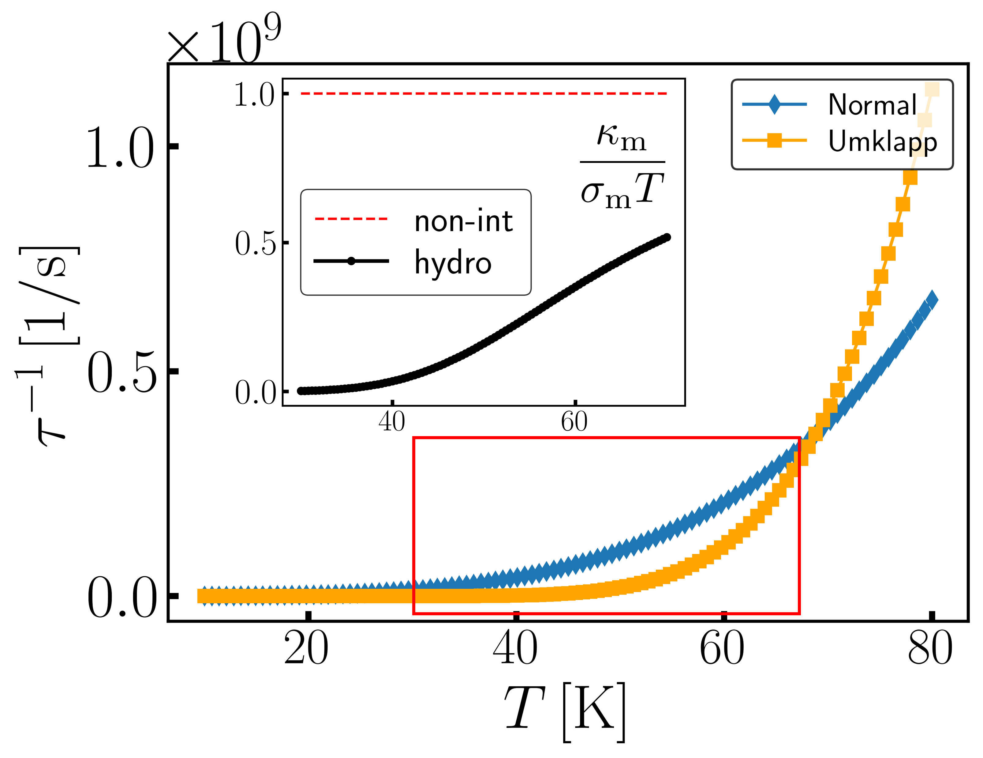
Figure 1: Breaking down the magnonic Wiedemann-Franz law. Temperature dependence of relaxation rates $\tau^{-1}$ for both Normal and Umklapp magnon-magnon scatterings are depicted. The red box shows the area satisfying $\tau_{\mathrm{N}}\ll\tau_{\mathrm{U}}$, namely, the hydrodynamic regime. The inset shows the ratio $\kappa_{\mathrm{m}}/\sigma_{\mathrm{m}}T|_{\mathrm{hydro}}$, calculated from Eq. (12) in units of the magnonic Lorenz number $\kappa_{\mathrm{m}}/\sigma_{\mathrm{m}}T|_{\mathrm{non-int}}$. When the system enters the hydrodynamic regime, the ratio shows a large deviation from unity.

Discussion.— Finally, we will discuss the experimental feasibility of the breakdown of the magnonic WF law. According to Refs. Bhandari and Verma (1966); Boona and Heremans (2014); Bender et al. (2014); Rückriegel et al. (2014), relaxation times are estimated as $\tau_{\mathrm{N}}^{-1}\sim(T/T_{\mathrm{e}})^{3}k_{\mathrm{B}}T/\hbar$ and $\tau_{\mathrm{U}}^{-1}\sim\sqrt{T/T_{\mathrm{e}}}\exp(-12T_{\mathrm{e}}/T)k_{\mathrm{B}}T/\hbar$ with $T_{\mathrm{e}}=2SJ/k_{\mathrm{B}}\sim 37$ K for yttrium-iron-garnet (YIG). The difference in temperature dependences of these two relaxation times originates from possible regions in reciprocal space under the scattering processes limited by overall conservation of energy and momentum modulo reciprocal lattice vectors Michel and Schwabl (1969, 1970); Ziman (1960); Forney and Jäckle (1973). Fig. [1] illustrates the temperature dependences of scattering rates $1/\tau$. The red box dictates the area satisfying $\tau_{\mathrm{N}}\ll\tau_{\mathrm{U}}$, namely, the hydrodynamic regime. The ratio $\kappa_{\mathrm{m}}/\sigma_{\mathrm{m}}T|_{\mathrm{hydro}}$ in units of the magnonic Lorenz number $\kappa_{\mathrm{m}}/\sigma_{\mathrm{m}}T|_{\mathrm{non-int}}$ is depicted in the inset of Fig. [1]. When the magnon system enters the hydrodynamic regime, the ratio shows a large deviation from unity, which in turn results in the drastic breakdown of the magnonic WF law. We should discuss the effect of the dipolar interactions in realistic magnets which violates the magnon number conservation. The magnon dumping rate due to the dipolar interactions is in the order of $10^{6}$ s^-1 Rodriguez-Nieva et al. (2022) and is much slower than $\tau^{-1}_{\mathrm{N}}$ and $\tau_{\mathrm{U}}^{-1}$ [see Fig. 1]. Therefore, we neglect the dipolar interactions here and the hydrodynamic description which includes the number conservation law is valid under the dynamics we are interested in.

As the system enters the collisionless regime where the hydrodynamic description is invalid, an emergent sound mode referred to as the zero-magnon mode appears in low dimensional Heisenberg ferromagnets Goll et al. (2020). Although it needs microscopic calculations and is beyond the scope of our study, the impact of the zero-magnon mode on the magnonic Lorenz number may be an interesting future work.

Conclusion.—In summary, we have developed a basic framework of magnon hydrodynamics for topologically trivial bulk FMI, which is composed of the hydrodynamic equations Eqs. (4) and the entropy production rate Eq. (5). Based on these equations, we have first investigated the dissipative magnon and heat currents, which obey the Onsager reciprocity relations, and then the thermal and spin conductivities. As a hallmark of the hydrodynamic regime, we have revealed that the ratio between the two conductivities shows a large deviation from the standard form so-called the magnonic WF law. Here, we have identified an origin of the drastic breakdown as the difference in relaxation processes between spin and heat currents, which is unique to the hydrodynamic regime. The violation of the magnonic WF law does not depend on the details of the magnon dispersion: a universal feature of the hydrodynamic regime. Therefore, our results may yield key evidence for the experimental realization and detection of magnon fluids in a wide range of materials.

Supplemental Materials for
“Breaking down the magnonic Wiedemann-Franz law in hydrodynamic regime”

Ryotaro Sano

Mamoru Matsuo

I Derivation of the hydrodynamic equations for Magnon Fluids

I.1 I. Boltzmann Equation

In this section, we outline how to derive the conservation laws for magnon fluids. We start from the magnon Boltzmann equation,

$$\partialderivative{n_{{\bf\it k}}({\bf\it r},t)}{t}+\dot{{\bf\it r}}\dotproduct\partialderivative{n_{{\bf\it k}}({\bf\it r},t)}{{\bf\it r}}+\dot{{\bf\it k}}\dotproduct\partialderivative{n_{{\bf\it k}}({\bf\it r},t)}{{\bf\it k}}=\mathcal{C}[n_{{\bf\it k}}],$$ (S.13)

which governs the evolution of the magnon distribution function $n_{{\bf\it k}}({\bf\it r},t)$ in the phase space. The semiclassical equations of motion for magnons read

$$\dot{{\bf\it r}}=\partialderivative{\omega_{{\bf\it k}}}{{\bf\it k}},\qquad\dot{{\bf\it k}}=0,$$ (S.14)

where the external driving force is absent for simplicity. $\hbar\omega_{{\bf\it k}}$ is the energy of the magnon with the momentum ${\bf\it k}$. The collision integral $\mathcal{C}$ is divided into the contribution of normal (N) process and Umklapp (U) one in the usual manner,

$$\mathcal{C}[n_{{\bf\it k}}]=\mathcal{C}^{\mathrm{mm}}_{\mathrm{N}}[n_{{\bf\it k}}]+\mathcal{C}^{\mathrm{mm}}_{\mathrm{U}}[n_{{\bf\it k}}].$$ (S.15)

Note that we only consider magnon number-conserving scatterings in the following. For an interacting magnon gas, the collision integral for N process under the first Born approximation is given by  Hau (2008)

$$\mathcal{C}^{\mathrm{mm}}_{\mathrm{N}}[n_{{\bf\it k}}]=\int[\differential{{\bf\it k}^{\prime}}]\int[\differential{{\bf\it k}_{1}}]\int[\differential{{\bf\it k}_{1}^{\prime}}]w^{\mathrm{mm}}_{\mathrm{N}}({\bf\it k},{\bf\it k}_{1};{\bf\it k}^{\prime},{\bf\it k}^{\prime}_{1})[(1+n_{{\bf\it k}})(1+n_{{\bf\it k}_{1}})n_{{\bf\it k}^{\prime}}n_{{\bf\it k}_{1}^{\prime}}-n_{{\bf\it k}}n_{{\bf\it k}_{1}}(1+n_{{\bf\it k}^{\prime}})(1+n_{{\bf\it k}_{1}^{\prime}})],$$ (S.16)

where the intrinsic transition probability per unit time is

$$w^{\mathrm{mm}}_{\mathrm{N}}({\bf\it k},{\bf\it k}_{1};{\bf\it k}^{\prime},{\bf\it k}^{\prime}_{1})=\frac{2\pi}{\hbar}\frac{1}{2}\absolutevalue{W^{\mathrm{mm}}({\bf\it k},{\bf\it k}_{1};{\bf\it k}^{\prime},{\bf\it k}^{\prime}_{1})+W^{\mathrm{mm}}({\bf\it k}_{1},{\bf\it k},{\bf\it k}_{1}^{\prime},{\bf\it k}^{\prime})}^{2}\delta(\hbar\omega_{{\bf\it k}}+\hbar\omega_{{\bf\it k}_{1}}-\hbar\omega_{{\bf\it k}^{\prime}}-\hbar\omega_{{\bf\it k}^{\prime}_{1}})\delta({\bf\it k}+{\bf\it k}_{1}-{\bf\it k}^{\prime}-{\bf\it k}^{\prime}_{1}).$$ (S.17)

Here, $W({\bf\it k},{\bf\it k}_{1};{\bf\it k}^{\prime},{\bf\it k}_{1}^{\prime})=\matrixelement{{\bf\it k},{\bf\it k}_{1}}{\hat{W}}{{\bf\it k}^{\prime},{\bf\it k}_{1}^{\prime}}$ is the interaction matrix element. Eq. (S.17) shows that N process conserves both energy and momentum during the collisions. On the other hand, we assume the relaxation approximation for the U process which does not conserve the momentum,

$$\mathcal{C}^{\mathrm{mm}}_{\mathrm{U}}[n_{{\bf\it k}}]=-\frac{n_{{\bf\it k}}({\bf\it r},t)-N_{{\bf\it k}}({\bf\it r},t)}{\tau_{\mathrm{U}}}.$$ (S.18)

Therefore, U processes tend to relax the magnon populations towards local thermal equilibrium $N_{{\bf\it k}}$.

We introduce an arbitrary function $\mathcal{N}({\bf\it k},n_{{\bf\it k}})$ which depends on the momentum ${\bf\it k}$ and the distribution $n_{{\bf\it k}}$. Its local density is defined as

$$\langle\mathcal{N}({\bf\it r},t)\rangle\equiv\int[\differential{{\bf\it k}}]\mathcal{N}({\bf\it k},n_{{\bf\it k}})n_{{\bf\it k}}.$$ (S.19)

The change of this function due to the N collisions is calculated as

$$\left.\partialderivative{\langle\mathcal{N}({\bf\it r},t)\rangle}{t}\right|_{\mathrm{coll:N}} =\int[\differential{{\bf\it k}}]\left.\partialderivative{[\mathcal{N}({\bf\it k},n_{{\bf\it k}})n_{{\bf\it k}}]}{t}\right|_{\mathrm{coll:N}}=\int[\differential{{\bf\it k}}]\mathcal{C}^{\mathrm{mm}}_{\mathrm{N}}[n_{{\bf\it k}}]\partialderivative{[\mathcal{N}({\bf\it k},n_{{\bf\it k}})n_{{\bf\it k}}]}{n_{{\bf\it k}}}$$

$$=\int[\differential{{\bf\it k}}]\int[\differential{{\bf\it k}^{\prime}}]\int[\differential{{\bf\it k}_{1}}]\int[\differential{{\bf\it k}_{1}^{\prime}}]w_{\mathrm{N}}^{\mathrm{mm}}({\bf\it k},{\bf\it k}_{1};{\bf\it k}^{\prime},{\bf\it k}_{1}^{\prime})\partialderivative{[\mathcal{N}({\bf\it k},n_{{\bf\it k}})n_{{\bf\it k}}]}{n_{{\bf\it k}}}$$

$$\times[(1+n_{{\bf\it k}})(1+n_{{\bf\it k}_{1}})n_{{\bf\it k}^{\prime}}n_{{\bf\it k}_{1}^{\prime}}-n_{{\bf\it k}}n_{{\bf\it k}_{1}}(1+n_{{\bf\it k}^{\prime}})(1+n_{{\bf\it k}_{1}^{\prime}})].$$ (S.20)

Exploiting the symmetry of the intrinsic transition probability $w_{\mathrm{N}}^{\mathrm{mm}}({\bf\it k},{\bf\it k}_{1};{\bf\it k}^{\prime},{\bf\it k}_{1}^{\prime})$ with respect to the exchange of particle coordinates

$$w_{\mathrm{N}}^{\mathrm{mm}}({\bf\it k},{\bf\it k}_{1};{\bf\it k}^{\prime},{\bf\it k}_{1}^{\prime}) =w_{\mathrm{N}}^{\mathrm{mm}}({\bf\it k}_{1},{\bf\it k};{\bf\it k}^{\prime}_{1},{\bf\it k}^{\prime})$$ (S.21a)

$$=w_{\mathrm{N}}^{\mathrm{mm}}({\bf\it k}^{\prime},{\bf\it k}^{\prime}_{1};{\bf\it k},{\bf\it k}_{1})=w_{\mathrm{N}}^{\mathrm{mm}}({\bf\it k}_{1}^{\prime},{\bf\it k}^{\prime};{\bf\it k}_{1},{\bf\it k}),$$ (S.21b)

Eq. (S.20) is rewritten as

$$\int[\differential{{\bf\it k}}]\mathcal{C}^{\mathrm{mm}}_{\mathrm{N}}[n_{{\bf\it k}}]\partialderivative{[\mathcal{N}({\bf\it k},n_{{\bf\it k}})n_{{\bf\it k}}]}{n_{{\bf\it k}}} =\frac{1}{4}\int[\differential{{\bf\it k}}]\int[\differential{{\bf\it k}^{\prime}}]\int[\differential{{\bf\it k}_{1}}]\int[\differential{{\bf\it k}_{1}^{\prime}}]w_{\mathrm{N}}^{\mathrm{mm}}({\bf\it k},{\bf\it k}_{1};{\bf\it k}^{\prime},{\bf\it k}_{1}^{\prime})$$

$$\times\left\{\partialderivative{[\mathcal{N}({\bf\it k},n_{{\bf\it k}})n_{{\bf\it k}}]}{n_{{\bf\it k}}}+\partialderivative{[\mathcal{N}({\bf\it k}_{1},n_{{\bf\it k}_{1}})n_{{\bf\it k}_{1}}]}{n_{{\bf\it k}_{1}}}-\partialderivative{[\mathcal{N}({\bf\it k}^{\prime},n_{{\bf\it k}^{\prime}})n_{{\bf\it k}^{\prime}}]}{n_{{\bf\it k}^{\prime}}}-\partialderivative{[\mathcal{N}({\bf\it k}^{\prime}_{1},n_{{\bf\it k}_{1}^{\prime}})n_{{\bf\it k}_{1}^{\prime}}]}{n_{{\bf\it k}_{1}^{\prime}}}\right\}$$

$$\times[(1+n_{{\bf\it k}})(1+n_{{\bf\it k}_{1}})n_{{\bf\it k}^{\prime}}n_{{\bf\it k}_{1}^{\prime}}-n_{{\bf\it k}}n_{{\bf\it k}_{1}}(1+n_{{\bf\it k}^{\prime}})(1+n_{{\bf\it k}_{1}^{\prime}})].$$ (S.22)

I.2 II. H-Theorem

Now we consider the following choice for $\mathcal{N}$:

$$\mathcal{N}({\bf\it k},n_{{\bf\it k}})n_{{\bf\it k}}=(1+n_{{\bf\it k}})\log(1+n_{{\bf\it k}})-n_{{\bf\it k}}\log n_{{\bf\it k}}.$$ (S.23)

The partial derivative with respect to $n_{{\bf\it k}}$ yields

$$\partialderivative{[\mathcal{N}({\bf\it k},n_{{\bf\it k}})n_{{\bf\it k}}]}{n_{{\bf\it k}}}=\log\frac{n_{{\bf\it k}}}{1+n_{{\bf\it k}}},$$ (S.24)

and Eq. (S.22) becomes

$$\int[\differential{{\bf\it k}}]\mathcal{C}^{\mathrm{mm}}_{\mathrm{N}}[n_{{\bf\it k}}]\partialderivative{[\mathcal{N}({\bf\it k},n_{{\bf\it k}})n_{{\bf\it k}}]}{n_{{\bf\it k}}} =-\frac{1}{4}\int[\differential{{\bf\it k}}]\int[\differential{{\bf\it k}^{\prime}}]\int[\differential{{\bf\it k}_{1}}]\int[\differential{{\bf\it k}_{1}^{\prime}}]w_{\mathrm{N}}^{\mathrm{mm}}({\bf\it k},{\bf\it k}_{1};{\bf\it k}^{\prime},{\bf\it k}_{1}^{\prime})\log\left[\frac{(1+n_{{\bf\it k}})(1+n_{{\bf\it k}_{1}})n_{{\bf\it k}^{\prime}}n_{{\bf\it k}_{1}^{\prime}}}{n_{{\bf\it k}}n_{{\bf\it k}_{1}}(1+n_{{\bf\it k}^{\prime}})(1+n_{{\bf\it k}^{\prime}_{1}})}\right]$$

$$\times[(1+n_{{\bf\it k}})(1+n_{{\bf\it k}_{1}})n_{{\bf\it k}^{\prime}}n_{{\bf\it k}_{1}^{\prime}}-n_{{\bf\it k}}n_{{\bf\it k}_{1}}(1+n_{{\bf\it k}^{\prime}})(1+n_{{\bf\it k}_{1}^{\prime}})]$$

$$\equiv\left.\partialderivative{H({\bf\it r},t)}{t}\right|_{\mathrm{coll:N}}.$$ (S.25)

The integrand is of the form $(x-y)\log(x/y)$, and hence nonnegative. Thus, the H-function always decrease in the approach to equilibrium. This is the famaous Boltzmann’s H-theorem.

The H-theorem shows that the entropy density, which for a Bose gas is given by

$$s({\bf\it r},t) \equiv-k_{\mathrm{B}}H({\bf\it r},t)$$ (S.26a)

$$=-k_{\mathrm{B}}\int[\differential{{\bf\it k}}]\Bigl{\{}(1+n_{{\bf\it k}})\log(1+n_{{\bf\it k}})-n_{{\bf\it k}}\log n_{{\bf\it k}}\Bigr{\}},$$ (S.26b)

reaches a maximum in equilibrium. Here, $k_{\mathrm{B}}$ is Boltzmann’s constant.

I.3 III. Collision Invariants

We will show that the Boltzmann equation Eq. (S.13) describes indeed an approach to the well-known Bose-Einstein equilibrium distribution. For this purpose, we first formalize the conservation laws. Here, we define the collision invariants $\mathcal{N}_{\lambda}$ as

$$\int[\differential{{\bf\it k}}]\mathcal{C}^{\mathrm{mm}}_{\mathrm{N}}[n_{{\bf\it k}}]\mathcal{N}_{\lambda}=0.$$ (S.27)

From this definition and Eq. (S.22), we immediately identify $\mathcal{N}_{\lambda}$ as,

$$\mathcal{N}_{0}=1,\qquad\mathcal{N}_{i}=\hbar k_{i},\qquad\mathcal{N}_{4}=\hbar\omega_{{\bf\it k}}.$$ (S.28)

Multiplying the Boltzmann equation Eq.(S.13) by the collision invariants $\mathcal{N}_{\lambda}$ gives the conservation laws for each invariant density respectively:

$$\partialderivative{t}\int[\differential{{\bf\it k}}]\mathcal{N}_{\lambda}n_{{\bf\it k}}+\divergence\int[\differential{{\bf\it k}}]\partialderivative{\omega_{{\bf\it k}}}{{\bf\it k}}\mathcal{N}_{\lambda}n_{{\bf\it k}}=\partialderivative{t}\langle\mathcal{N}_{\lambda}\rangle+\divergence{\bf\it\mathcal{J}}^{\mathcal{N}_{\lambda}}$$ (S.29a)

$$\quad=\int[\differential{{\bf\it k}}](\mathcal{C}^{\mathrm{mm}}_{\mathrm{N}}[n_{{\bf\it k}}]+\mathcal{C}^{\mathrm{mm}}_{\mathrm{U}}[n_{{\bf\it k}}])\mathcal{N}_{\lambda}=\int[\differential{{\bf\it k}}]\mathcal{C}^{\mathrm{mm}}_{\mathrm{U}}[n_{{\bf\it k}}]\mathcal{N}_{\lambda}=-\int[\differential{{\bf\it k}}]\frac{n_{{\bf\it k}}-N_{{\bf\it k}}}{\tau_{\mathrm{U}}}\mathcal{N}_{\lambda},$$ (S.29b)

where we have defined the invariant densities $$\langle\mathcal{N}_{\lambda}\rangle {\bf\it\mathcal{J}}^{\mathcal{N}_{\lambda}}$$ and corresponding fluxes as follows:

$$\langle\mathcal{N}_{\lambda}({\bf\it r},t)\rangle=\int[\differential{{\bf\it k}}]\mathcal{N}_{\lambda}n_{{\bf\it k}}({\bf\it r},t),\qquad{\bf\it\mathcal{J}}^{\mathcal{N}_{\lambda}}({\bf\it r},t)=\int[\differential{{\bf\it k}}]\partialderivative{\omega_{{\bf\it k}}}{{\bf\it k}}\mathcal{N}_{\lambda}n_{{\bf\it k}}({\bf\it r},t).$$ (S.29c)

I.4 IV. Local Equilibrium Distribution

The local equilibrium distribution $n_{{\bf\it k}}^{(0)}$ is derived from the term in square brackets in Eq. (S.25) has to vanish:

$$\log\frac{n^{(0)}_{{\bf\it k}}}{1+n^{(0)}_{{\bf\it k}}}+\log\frac{n^{(0)}_{{\bf\it k}_{1}}}{1+n^{(0)}_{{\bf\it k}_{1}}}=\log\frac{n^{(0)}_{{\bf\it k}^{\prime}}}{1+n^{(0)}_{{\bf\it k}^{\prime}}}+\log\frac{n^{(0)}_{{\bf\it k}^{\prime}_{1}}}{1+n^{(0)}_{{\bf\it k}^{\prime}_{1}}}.$$ (S.30)

This indicates that $\log[n^{(0)}/(1+n^{(0)})]$ is also a conserved quantity. Owing to basic conservation laws Eqs. (S.29) which we obtained, this quantity can be expressed as a linear combination of the collision invariants $\mathcal{N}_{\lambda}$:

$$\log\frac{n^{(0)}_{{\bf\it k}}}{1+n^{(0)}_{{\bf\it k}}}=-\sum_{\lambda}\beta_{\lambda}\mathcal{N}_{\lambda},$$ (S.31)

with

$$\beta_{0}=\frac{-\tilde{\mu}}{k_{\mathrm{B}}T},\qquad\beta_{i}=\frac{-{\bf\it v}}{k_{\mathrm{B}}T},\qquad\beta_{4}=\frac{1}{k_{\mathrm{B}}T},$$ (S.32)

where $\tilde{\mu}=\mu-m^{\ast}{\bf\it v}^{2}/2$ is the magnon chemical potential in the frame which moves with fluid and ${\bf\it v}$ is the drift velocity of the magnon system. All the expressions in Eq. (S.32) can be slowly varying functions of ${\bf\it r}$ and $t$. Such a situation is called a local equilibrium and Eq. (S.31) has the solution

$$n_{{\bf\it k}}^{(0)}({\bf\it r},t)=n_{\mathrm{B}}\biggl{(}\sum_{\lambda}\beta_{\lambda}({\bf\it r},t)\mathcal{N}_{\lambda}\biggr{)}=\left[\exp\left\{\frac{\hbar\omega_{{\bf\it k}}-\hbar{\bf\it k}\dotproduct{\bf\it v}({\bf\it r},t)-\tilde{\mu}({\bf\it r},t)}{k_{\mathrm{B}}T({\bf\it r},t)}\right\}-1\right]^{-1},$$ (S.33)

which is referred to as the local equilibrium distribution. Here, $n_{\mathrm{B}}(x)=1/(e^{x}-1)$ is the Bose-Einstein function and we use the quadratic dispersion for magnons $\hbar\omega_{{\bf\it k}}=\hbar^{2}{\bf\it k}^{2}/2m^{\ast}$ with the effective mass $m^{\ast}$. A similar derivation for the Boltzmann equation with U scattering process results in an equilibrium magnon distribution of the form

$$\qquad N_{{\bf\it k}}({\bf\it r},t)=\left[\exp\left\{\frac{\hbar\omega_{{\bf\it k}}-\mu({\bf\it r},t)}{k_{\mathrm{B}}T({\bf\it r},t)}\right\}-1\right]^{-1},$$ (S.34)

because the drift velocity of magnons, whose total momentum is not conserved, is identical to zero.

I.5 V. Hydrodynamic Equations

We are now ready to derive the hydrodynamic equations from the conservation laws Eqs. (S.29). In the following analysis, we assume that the local equilibrium distribution $n_{{\bf\it k}}^{(0)}$ is transformed into the equilibrium distribution $N_{{\bf\it k}}$ under the Galilean transformation from the frame in which the fluid moves with the velocity ${\bf\it v}$ to the frame in which it is at rest: $\hbar{\bf\it k}\to\hbar{\bf\it k}+m^{\ast}{\bf\it v}$.

I.5.1 Number Conservation

First, we start from the number conservation law by setting $\mathcal{N}_{0}=1$,

$$\langle\mathcal{N}_{0}\rangle =\int[\differential{{\bf\it k}}]n_{{\bf\it k}}\equiv n({\bf\it r},t),$$ (S.35a)

$${\bf\it\mathcal{J}}^{\mathcal{N}_{0}} =\int[\differential{{\bf\it k}}]\partialderivative{\omega_{{\bf\it k}}}{{\bf\it k}}n_{{\bf\it k}}=\int[\differential{{\bf\it k}}]\left(\partialderivative{\omega_{{\bf\it k}}}{{\bf\it k}}-{\bf\it v}\right)n_{{\bf\it k}}+{\bf\it v}\int[\differential{{\bf\it k}}]n_{{\bf\it k}}$$

$$={\bf\it J}+n({\bf\it r},t){\bf\it v}({\bf\it r},t).$$ (S.35b)

Here, we have defined $${\bf\it J}$$ as

$${\bf\it J}\equiv\int[\differential{{\bf\it k}}]\left(\partialderivative{\omega_{{\bf\it k}}}{{\bf\it k}}-{\bf\it v}\right)n_{{\bf\it k}},$$ (S.35c)

whose physical meaning becomes clear when we consider the entropy production.

After all, we obtain the number conservation law as follows:

$$\partialderivative{n}{t}+\divergence(n{\bf\it v}+{\bf\it J})=0.$$ (S.36)

I.5.2 Momentum Conservation

Next, we calculate the momentum conservation law by setting $\mathcal{N}_{i}=\hbar k_{i}$,

$$\langle\mathcal{N}_{i}\rangle =\int[\differential{{\bf\it k}}]\hbar k_{i}n_{{\bf\it k}}\equiv m^{\ast}nv_{i}\equiv\rho v_{i},$$ (S.37a)

$$\mathcal{J}_{j}^{\mathcal{N}_{i}} =\int[\differential{{\bf\it k}}]\partialderivative{\omega_{{\bf\it k}}}{k_{j}}\hbar k_{i}n_{{\bf\it k}}=\int[\differential{{\bf\it k}}]\left(\partialderivative{\omega_{{\bf\it k}}}{k_{j}}-v_{j}\right)\left(\hbar k_{i}-m^{\ast}v_{i}\right)n_{{\bf\it k}}+\int[\differential{{\bf\it k}}]\left(m^{\ast}\partialderivative{\omega_{{\bf\it k}}}{k_{j}}v_{i}+v_{j}\hbar k_{i}\right)n_{{\bf\it k}}-m^{\ast}v_{j}v_{i}\int[\differential{{\bf\it k}}]n_{{\bf\it k}}$$

$$=\Pi_{ji}+m^{\ast}\mathcal{J}_{j}^{\mathcal{N}_{0}}v_{i}+v_{j}\langle\mathcal{N}_{i}\rangle-\rho v_{j}v_{i}=\Pi_{ji}+m^{\ast}\mathcal{J}_{j}^{\mathcal{N}_{0}}v_{i},$$ (S.37b)

where we have defined the stress tensor as

$$\Pi_{ji}\equiv\int[\differential{{\bf\it k}}]\left(\partialderivative{\omega_{{\bf\it k}}}{k_{j}}-v_{j}\right)\left(\hbar k_{i}-m^{\ast}v_{i}\right)n_{{\bf\it k}}.$$ (S.37c)

Therefore, the balance equation for momentum is obtained as

$$\partialderivative{t}(\rho v_{i})+\partialderivative{x_{j}}\left[(\rho v_{j}+J_{j})v_{i}\right]+\partialderivative{x_{j}}\Pi_{ji}=-\frac{\rho v_{i}}{\tau_{\mathrm{U}}},$$ (S.38a)

or

$$\rho\partialderivative{v_{i}}{t}+(\rho v_{j}+J_{j})\partialderivative{v_{i}}{x_{j}}+\partialderivative{x_{j}}\Pi_{ji}=-\frac{\rho v_{i}}{\tau_{\mathrm{U}}},$$ (S.38b)

with the help of Eq. (S.36). Multiplying Eq. (S.38b) by $v_{i}$ and summing over $i$, we obtain the following relation,

$$\rho v_{i}\partialderivative{v_{i}}{t}+(\rho v_{j}+J_{j})v_{i}\partialderivative{v_{i}}{x_{j}} =\partialderivative{t}\left(\frac{\rho}{2}v_{i}v_{i}\right)+\partialderivative{x_{j}}\left[\left(\rho v_{j}+J_{j}\right)\frac{v_{i}v_{i}}{2}\right]-\frac{v_{i}v_{i}}{2}\underbrace{\left[\partialderivative{\rho}{t}+\partialderivative{x_{j}}(\rho v_{j}+J_{j})\right]}_{0}$$

$$=\partialderivative{t}\left(\frac{\rho}{2}v_{i}v_{i}\right)+\partialderivative{x_{j}}\left[(\rho v_{j}+J_{j})\frac{v_{i}v_{i}}{2}\right].$$ (S.39a)

Therefore, we can express Eq. (S.38b) in another form:

$$\partialderivative{t}\left(\frac{\rho}{2}v_{i}v_{i}\right)+\partialderivative{x_{j}}\left[(\rho v_{j}+J_{j})\frac{v_{i}v_{i}}{2}\right]+v_{i}\partialderivative{x_{j}}\Pi_{ji}=-\frac{\rho v_{i}v_{i}}{\tau_{\mathrm{U}}}.$$ (S.39b)

I.5.3 Energy conservation

Finally, we calculate the energy conservation law by setting $\mathcal{N}_{4}=\hbar\omega_{{\bf\it k}}$,

$$\langle\mathcal{N}_{4}\rangle =\int[\differential{{\bf\it k}}]\hbar\omega_{{\bf\it k}}n_{{\bf\it k}}=\int[\differential{{\bf\it k}}]\frac{(\hbar{\bf\it k}-m^{\ast}{\bf\it v})^{2}}{2m}n_{{\bf\it k}}+\int[\differential{{\bf\it k}}]\hbar k_{i}v_{i}n_{{\bf\it k}}-\frac{m^{\ast}}{2}{\bf\it v}^{2}\int[\differential{{\bf\it k}}]n_{{\bf\it k}}$$

$$=u+\langle\mathcal{N}_{i}\rangle v_{i}-\frac{\rho}{2}{\bf\it v}^{2}=u+\frac{\rho}{2}{\bf\it v}^{2},$$ (S.40a)

$$\mathcal{J}_{j}^{\mathcal{N}_{4}} \equiv\int[\differential{{\bf\it k}}]\partialderivative{\omega_{{\bf\it k}}}{k_{j}}\hbar\omega_{{\bf\it k}}n_{{\bf\it k}}$$

$$=\int[\differential{{\bf\it k}}]\left(\partialderivative{\omega_{{\bf\it k}}}{k_{j}}-v_{j}\right)\frac{(\hbar{\bf\it k}-m^{\ast}{\bf\it v})^{2}}{2m^{\ast}}n_{{\bf\it k}}+\int[\differential{{\bf\it k}}]\left(\partialderivative{\omega_{{\bf\it k}}}{k_{j}}-v_{j}\right)(\hbar{\bf\it k}-m^{\ast}{\bf\it v})\dotproduct{\bf\it v}n_{{\bf\it k}}+\frac{m^{\ast}}{2}{\bf\it v}^{2}\int[\differential{{\bf\it k}}]\left(\partialderivative{\omega_{{\bf\it k}}}{k_{j}}-v_{j}\right)n_{{\bf\it k}}$$

$$\quad+v_{j}\int[\differential{{\bf\it k}}]\hbar\omega_{{\bf\it k}}n_{{\bf\it k}}$$

$$=Q_{j}+\Pi_{ji}v_{i}+\frac{{\bf\it v}^{2}}{2}(\mathcal{J}_{j}^{\mathcal{N}_{0}}-\rho v_{j})+\langle\mathcal{N}_{4}\rangle v_{j}=Q_{j}+\Pi_{ji}v_{i}+\frac{{\bf\it v}^{2}}{2}J_{j}+\left(u+\frac{\rho}{2}{\bf\it v}^{2}\right)v_{j},$$ (S.40b)

where we have defined the internal energy density $$u {\bf\it Q}$$ and the heat current as

$$u\equiv\int[\differential{{\bf\it k}}]\frac{(\hbar{\bf\it k}-m^{\ast}{\bf\it v})^{2}}{2m^{\ast}}n_{{\bf\it k}},\qquad{\bf\it Q}\equiv\int[\differential{{\bf\it k}}]\left(\partialderivative{\omega_{{\bf\it k}}}{{\bf\it k}}-{\bf\it v}\right)\frac{(\hbar{\bf\it k}-m^{\ast}{\bf\it v})^{2}}{2m^{\ast}}n_{{\bf\it k}}.$$ (S.40c)

Therefore, the energy conservation law becomes

$$\partialderivative{t}\left(u+\frac{\rho}{2}{\bf\it v}^{2}\right)+\partialderivative{x_{j}}\left[uv_{j}+Q_{j}+(\rho v_{j}+J_{j})\frac{{\bf\it v}^{2}}{2}\right]+\partialderivative{x_{j}}(\Pi_{ji}v_{i})=0,$$ (S.41)

or

$$\partialderivative{u}{t}+\divergence(u{\bf\it v}+{\bf\it Q})+\Pi_{ji}\partialderivative{x_{j}}v_{i}=\frac{\rho v_{i}v_{i}}{\tau_{\mathrm{U}}},$$ (S.42)

by employing Eq. (S.39b).

I.6 VI. Deviation from the Local Equilibrium Distribution

By considering the deviation from the local equilibrium distribution as $n_{{\bf\it k}}^{\prime}=n_{{\bf\it k}}-n_{{\bf\it k}}^{(0)}$, the fluxes for each conserved quantity are devided into two contribution:

$${\bf\it J}={\bf\it J}^{(0)}+{\bf\it J}^{\prime},\qquad\Pi_{ji}=\Pi^{(0)}_{ji}+\Pi_{ji}^{\prime},\qquad{\bf\it Q}={\bf\it Q}^{(0)}+{\bf\it Q}^{\prime},$$ (S.43a)

with

$${\bf\it J}^{(0)} =\int[\differential{{\bf\it k}}]\left(\partialderivative{\omega_{{\bf\it k}}}{{\bf\it k}}-{\bf\it v}\right)n_{{\bf\it k}}^{(0)}=\int[\differential{{\bf\it k}}]\partialderivative{\omega_{{\bf\it k}}}{{\bf\it k}}N_{{\bf\it k}}=0,$$ (S.43b)

$$\Pi_{ji}^{(0)} =\int[\differential{{\bf\it k}}]\left(\partialderivative{\omega_{{\bf\it k}}}{k_{j}}-v_{j}\right)\left(\hbar k_{i}-m^{\ast}v_{i}\right)n_{{\bf\it k}}^{(0)}=\int[\differential{{\bf\it k}}]\partialderivative{\omega_{{\bf\it k}}}{k_{j}}\hbar k_{i}N_{{\bf\it k}}=P\delta_{ij},$$ (S.43c)

$${\bf\it Q}^{(0)} =\int[\differential{{\bf\it k}}]\left(\partialderivative{\omega_{{\bf\it k}}}{{\bf\it k}}-{\bf\it v}\right)\frac{(\hbar{\bf\it k}-m^{\ast}{\bf\it v})^{2}}{2m^{\ast}}n^{(0)}_{{\bf\it k}}=\int[\differential{{\bf\it k}}]\partialderivative{\omega_{{\bf\it k}}}{{\bf\it k}}\frac{(\hbar{\bf\it k})^{2}}{2m^{\ast}}N_{{\bf\it k}}=0,$$ (S.43d)

where we have introduced the pressure $$P$$ as

$$P\equiv-k_{\mathrm{B}}T\int[\differential{{\bf\it k}}]\log[1-e^{-\beta(\hbar\omega_{{\bf\it k}}-\mu)}].$$ (S.43e)

By using these quantities, the hydrodynamic equations Eqs. (S.39b) and  (S.42) are rewritten as

$$\rho\partialderivative{v_{i}}{t}+(\rho v_{j}+J_{j}^{\prime})\partialderivative{v_{i}}{x_{j}}+\partialderivative{x_{i}}P+\partialderivative{x_{j}}\Pi_{ji}^{\prime}=-\frac{\rho v_{i}}{\tau_{\mathrm{U}}},$$ (S.44)

$$\partialderivative{u}{t}+\divergence(u{\bf\it v})+P\divergence{\bf\it v}+\divergence{\bf\it Q}^{\prime}+\Pi^{\prime}_{ji}\partialderivative{v_{i}}{x_{j}}=\frac{\rho{\bf\it v}^{2}}{\tau_{\mathrm{U}}}.$$ (S.45)

Comparing with the phenomelogical hydrodynamics, ${\bf\it J}^{\prime}$, $\Pi_{ji}^{\prime}$, and $\mathbf{Q}^{\prime}$ correspond to the diffusion current, the viscous stress, and the heat current respectively. Namely, dissipative currents emerge only when considering the deviation from the local equilibrium.

II Entropy production

By employing nonequilibrium thermodynamics, we first assume that the Gibbs-Duhem equation

$$Ts=u+P-\mu n,$$ (S.46)

and the thermodynamic relation

$$s\differential{T}=\differential{P}-n\differential{\mu}.$$ (S.47)

Then, we rewrite Eq. (S.46) by using our invariant densities as

$$Ts=\langle\mathcal{N}_{4}\rangle-\langle\mathcal{N}_{i}\rangle v_{i}+P-\tilde{\mu}\langle\mathcal{N}_{0}\rangle.$$ (S.48)

From Eqs. (S.47) and  (S.48), we obtain

$$T\differential{s} =\differential{u}-\mu\differential{n}$$

$$=\differential{\langle\mathcal{N}_{4}\rangle}-v_{i}\differential{\langle\mathcal{N}_{i}\rangle}-\tilde{\mu}\differential{\langle\mathcal{N}_{0}\rangle}.$$ (S.49)

From this equation, we obtain the following relations,

$$\partialderivative{s}{t} =\frac{1}{T}\partialderivative{\langle\mathcal{N}_{4}\rangle}{t}-\frac{v_{i}}{T}\partialderivative{\langle\mathcal{N}_{i}\rangle}{t}-\frac{\tilde{\mu}}{T}\partialderivative{\mathcal{N}_{0}}{t},$$ (S.50a)

$$\gradient s =\frac{1}{T}\gradient\langle\mathcal{N}_{4}\rangle-\frac{v_{i}}{T}\gradient\langle\mathcal{N}_{i}\rangle-\frac{\tilde{\mu}}{T}\gradient\mathcal{N}_{0},$$ (S.50b)

By using the conservation laws we derived, we construct the entropy production equation as follows:

$$\partialderivative{s}{t}+\divergence(s{\bf\it v})=\partialderivative{s}{t}+s\divergence{\bf\it v}+{\bf\it v}\dotproduct\gradient s$$

$$=-\divergence\frac{({\bf\it\mathcal{J}}^{\mathcal{N}_{4}}-\langle\mathcal{N}_{4}\rangle{\bf\it v})-v_{i}({\bf\it\mathcal{J}}^{\mathcal{N}_{i}}-\langle\mathcal{N}_{i}\rangle{\bf\it v})-\tilde{\mu}({\bf\it\mathcal{J}}^{\mathcal{N}_{0}}-\langle\mathcal{N}_{0}\rangle{\bf\it v})}{T}$$

$$\quad+({\bf\it\mathcal{J}}^{\mathcal{N}_{4}}-\langle\mathcal{N}_{4}\rangle{\bf\it v})\dotproduct\gradient\left(\frac{1}{T}\right)+\frac{P}{T}(\divergence{\bf\it v})+({\bf\it\mathcal{J}}^{\mathcal{N}_{i}}-\langle\mathcal{N}_{i}\rangle{\bf\it v})\dotproduct\gradient\left(-\frac{v_{i}}{T}\right)+({\bf\it\mathcal{J}}^{\mathcal{N}_{0}}-\langle\mathcal{N}_{0}\rangle{\bf\it v})\dotproduct\gradient\left(-\frac{\tilde{\mu}}{T}\right).$$ (S.51)

Substituting the form of hydrodynamic variables into each invariant density and corresponding flux, the entropy production rate becomes

$$\partialderivative{s}{t}+\divergence\left(s{\bf\it v}+\frac{{\bf\it Q}^{\prime}-{\mu}{\bf\it J}^{\prime}}{T}\right)$$

$$={\bf\it Q}^{\prime}\dotproduct\gradient\left(\frac{1}{T}\right)+\frac{\Pi_{ji}^{\prime}}{T}\partial_{j}(-v_{i})+{\bf\it J}^{\prime}\dotproduct\gradient\left(-\frac{\mu}{T}\right)+\frac{1}{T}\frac{\rho{\bf\it v}^{2}}{\tau_{\mathrm{U}}},$$ (S.52a)

$$=\frac{{\bf\it Q}^{\prime}-{\mu}{\bf\it J}^{\prime}}{T}\dotproduct\left(-\frac{\gradient T}{T}\right)+\frac{\Pi_{ji}^{\prime}}{T}\gradient_{j}(-v_{i})+\frac{{\bf\it J}^{\prime}}{T}\dotproduct\gradient(-{\mu})+\frac{1}{T}\frac{\rho{\bf\it v}^{2}}{\tau_{\mathrm{U}}}.$$ (S.52b)

As can be seen, the entropy is irreversively produced by the dissipation currents stem from the deviation from the local equilibrium. The entropy production rate Eq. (S.52b) is given by the product of dissipation currents and corresponding thermodynamic forces:

$$\left(\partialderivative{s}{t}\right)_{\mathrm{irr}}=\sum_{i}Y_{i}X_{i}.$$ (S.53)

If we write the response of the general currents $Y_{i}$ induced by such thermodynamic forces $X_{i}$ as

$$Y_{i}=\sum_{j}\mathcal{L}_{ij}X_{i},$$ (S.54)

the response coefficients $\mathcal{L}_{ij}$ becomes symmetric $\mathcal{L}_{ij}=\mathcal{L}_{ji}$, which is well-known as the Onsager’s reciprocal relations.

III Heat current

In this section, we derive the heat current by considering deviation from the local equilibrium distribution $n_{{\bf\it k}}^{(0)}$. In the following analysis, we also assume the relaxation approximation for N process:

$$C_{\mathrm{N}}^{\mathrm{mm}}[n_{{\bf\it k}}]=-\frac{n_{{\bf\it k}}({\bf\it r},t)-n^{(0)}_{{\bf\it k}}({\bf\it r},t)}{\tau_{\mathrm{N}}}.$$ (S.55)

For the purpose of obtaining the spin and thermal conductivities, we expand the magnon distribution function around local equilibrium: $n_{{\bf\it k}}=n_{{\bf\it k}}^{(0)}+\delta n_{{\bf\it k}}$. Assuming that the deviation from local equilibrium is small to justify the use of the linearized Boltzmann equation, we can calculate $\delta n_{{\bf\it k}}$ by neglecting its time and spacial derivatives,

$$\left(\partialderivative{t}+\partialderivative{\omega_{{\bf\it k}}}{{\bf\it k}}\dotproduct\gradient\right)n_{{\bf\it k}}\simeq\left(\partialderivative{t}+\partialderivative{\omega_{{\bf\it k}}}{{\bf\it k}}\dotproduct\gradient\right)n_{{\bf\it k}}^{(0)}$$

$$\quad=-\frac{\delta n_{{\bf\it k}}}{\tau_{\mathrm{N}}}-\frac{n_{{\bf\it k}}^{(0)}+\delta n_{{\bf\it k}}-N_{{\bf\it k}}}{\tau_{\mathrm{U}}}=-\left(\frac{1}{\tau_{\mathrm{N}}}+\frac{1}{\tau_{\mathrm{U}}}\right)\delta n_{{\bf\it k}}-\frac{n_{{\bf\it k}}^{(0)}-N_{{\bf\it k}}}{\tau_{\mathrm{U}}}.$$ (S.56a)

Therefore, we obtain the deviation $$\delta n_{{\bf\it k}}$$ in the first approximation as,

$$\delta n_{{\bf\it k}}\simeq-\left(\frac{1}{\tau_{\mathrm{N}}}+\frac{1}{\tau_{\mathrm{U}}}\right)^{-1}\left[\left(\partialderivative{t}+\partialderivative{\omega_{{\bf\it k}}}{{\bf\it k}}\dotproduct\gradient\right)n_{{\bf\it k}}^{(0)}+\frac{n_{{\bf\it k}}^{(0)}-N_{{\bf\it k}}}{\tau_{\mathrm{U}}}\right].$$ (S.56b)

Furthermore, we assume that $\delta n_{{\bf\it k}}$ satisfies the following condition,

$$\int[\differential{{\bf\it k}}]\mathcal{N}_{\lambda}\delta n_{{\bf\it k}}=0,$$ (S.57a)

which results in the fact that the invariant densities is determined only by the local distribution function:

$$\langle\mathcal{N}_{\lambda}\rangle=\int[\differential{{\bf\it k}}]\mathcal{N}_{\lambda}(n_{{\bf\it k}}^{(0)}+\delta n_{{\bf\it k}})=\int[\differential{{\bf\it k}}]\mathcal{N}_{\lambda}n_{{\bf\it k}}^{(0)}=\langle\mathcal{N}_{\lambda}\rangle^{(0)}.$$ (S.57b)

This condition is necessary for not violating the conservation laws under the relaxation time approximation for N process. In the following analysis, we restrict ourselves to steady states and therefore neglect the time derivative $\partial/\partial t$ in Eq. (S.56b).

By substituting Eq. (S.56b) into Eq. (S.40c), we can calculate the heat current as,

$${\bf\it Q} =\int[\differential{{\bf\it k}}]\left(\partialderivative{\omega_{{\bf\it k}}}{{\bf\it k}}-{\bf\it v}\right)\frac{(\hbar{\bf\it k}-m^{\ast}{\bf\it v})^{2}}{2m^{\ast}}\delta n_{{\bf\it k}}$$

$$\simeq-\left(\frac{1}{\tau_{\mathrm{N}}}+\frac{1}{\tau_{\mathrm{U}}}\right)^{-1}\int[\differential{{\bf\it k}}]\left(\partialderivative{\omega_{{\bf\it k}}}{{\bf\it k}}-{\bf\it v}\right)\frac{(\hbar{\bf\it k}-m^{\ast}{\bf\it v})^{2}}{2m^{\ast}}\left[\partialderivative{\omega_{{\bf\it k}}}{{\bf\it k}}\dotproduct\gradient n_{{\bf\it k}}^{(0)}+\frac{n_{{\bf\it k}}^{(0)}-N_{{\bf\it k}}}{\tau_{\mathrm{U}}}\right]$$

$$\equiv{\bf\it Q}^{\gradient}+{\bf\it Q}^{\tau}.$$ (S.58a)

Here we have defined $${\bf\it Q}^{\gradient} {\bf\it Q}^{\tau}$$ and as

$${\bf\it Q}^{\gradient} \equiv-\left(\frac{1}{\tau_{\mathrm{N}}}+\frac{1}{\tau_{\mathrm{U}}}\right)^{-1}\int[\differential{{\bf\it k}}]\left(\partialderivative{\omega_{{\bf\it k}}}{{\bf\it k}}-{\bf\it v}\right)\frac{(\hbar{\bf\it k}-m^{\ast}{\bf\it v})^{2}}{2m^{\ast}}\partialderivative{\omega_{{\bf\it k}}}{{\bf\it k}}\dotproduct\gradient n_{{\bf\it k}}^{(0)},$$ (S.58b)

$${\bf\it Q}^{\tau} \equiv-\left(\frac{1}{\tau_{\mathrm{N}}}+\frac{1}{\tau_{\mathrm{U}}}\right)^{-1}\int[\differential{{\bf\it k}}]\left(\partialderivative{\omega_{{\bf\it k}}}{{\bf\it k}}-{\bf\it v}\right)\frac{(\hbar{\bf\it k}-m^{\ast}{\bf\it v})^{2}}{2m^{\ast}}\frac{n_{{\bf\it k}}^{(0)}-N_{{\bf\it k}}}{\tau_{\mathrm{U}}}.$$ (S.58c)

The contribution from U process ${\bf\it Q}^{\tau}$ can be easily calculated by using the relation Eq. (S.43d) as,

$${\bf\it Q}^{\tau} =\frac{1}{\tau_{\mathrm{U}}}\left(\frac{1}{\tau_{\mathrm{N}}}+\frac{1}{\tau_{\mathrm{U}}}\right)^{-1}\int[\differential{{\bf\it k}}]\left(\partialderivative{\omega_{{\bf\it k}}}{{\bf\it k}}-{\bf\it v}\right)\frac{(\hbar{\bf\it k}-m^{\ast}{\bf\it v})^{2}}{2m^{\ast}}N_{{\bf\it k}}$$

$$=\frac{-1}{\tau_{\mathrm{U}}}\left(\frac{1}{\tau_{\mathrm{N}}}+\frac{1}{\tau_{\mathrm{U}}}\right)^{-1}\int[\differential{{\bf\it k}}]\left\{\frac{(\hbar{\bf\it k})^{2}}{2m^{\ast}}{\bf\it v}+{\partialderivative{\omega_{{\bf\it k}}}{{\bf\it k}}}(\hbar{\bf\it k}\dotproduct{\bf\it v})+\left(\frac{m^{\ast}}{2}{\bf\it v}^{2}\right){\bf\it v}\right\}N_{{\bf\it k}}$$

$$=\frac{-1}{\tau_{\mathrm{U}}}\left(\frac{1}{\tau_{\mathrm{N}}}+\frac{1}{\tau_{\mathrm{U}}}\right)^{-1}\left(u^{(0)}+P+\frac{\rho^{(0)}}{2}{\bf\it v}^{2}\right){\bf\it v}.$$ (S.59)

On the other hand, the contribution from spatial gradients ${\bf\it Q}^{\gradient}$ needs to identify the spatial dependence of $n_{{\bf\it k}}^{(0)}$. $n_{{\bf\it k}}^{(0)}$ depends on space through $\tilde{\mu}$, ${\bf\it v}$, and $T$, thus $\gradient n_{{\bf\it k}}^{(0)}$ can be calculated as,

$$\gradient n_{{\bf\it k}}^{(0)} =\sum_{\lambda}\partialderivative{n_{{\bf\it k}}^{(0)}}{\beta_{\lambda}}\gradient\beta_{\lambda}$$

$$=\biggl{[}\sum_{\lambda}\mathcal{N}_{\lambda}\gradient\beta_{\lambda}\biggr{]}\left.\partialderivative{n_{\mathrm{B}}(x)}{x}\right|_{x=\sum_{\lambda}\beta_{\lambda}\mathcal{N}_{\lambda}}$$

$$=T\left[\hbar\omega_{{\bf\it k}}\gradient\left(\frac{1}{T}\right)+\hbar k_{j}\gradient\left(-\frac{v_{j}}{T}\right)+\gradient\left(-\frac{\tilde{\mu}}{T}\right)\right]\partialderivative{n_{{\bf\it k}}^{(0)}}{(\hbar\omega_{{\bf\it k}})}.$$ (S.60)

Therefore, ${\bf\it Q}^{\gradient}$ is further decomposed into three contributions: ${\bf\it Q}^{\gradient}={\bf\it Q}^{\gradient T}+{\bf\it Q}^{\gradient{\bf\it v}}+{\bf\it Q}^{\gradient\mu}$,

$${\bf\it Q}^{\gradient T} =-\left(\frac{1}{\tau_{\mathrm{N}}}+\frac{1}{\tau_{\mathrm{U}}}\right)^{-1}T\int[\differential{{\bf\it k}}]\left(\partialderivative{\omega_{{\bf\it k}}}{{\bf\it k}}-{\bf\it v}\right)\frac{(\hbar{\bf\it k}-m^{\ast}{\bf\it v})^{2}}{2m^{\ast}}\hbar\omega_{{\bf\it k}}\left\{\partialderivative{\omega_{{\bf\it k}}}{{\bf\it k}}\dotproduct\gradient\left(\frac{1}{T}\right)\right\}\partialderivative{n_{{\bf\it k}}^{(0)}}{(\hbar\omega_{{\bf\it k}})}$$

$$=-\left(\frac{1}{\tau_{\mathrm{N}}}+\frac{1}{\tau_{\mathrm{U}}}\right)^{-1}T\int[\differential{{\bf\it k}}]\left(\partialderivative{\omega_{{\bf\it k}}}{{\bf\it k}}-{\bf\it v}\right)\frac{(\hbar{\bf\it k}-m^{\ast}{\bf\it v})^{2}}{2m^{\ast}}\frac{(\hbar{\bf\it k}-m^{\ast}{\bf\it v})^{2}}{2m^{\ast}}\left\{\left(\partialderivative{\omega_{{\bf\it k}}}{{\bf\it k}}-{\bf\it v}\right)\dotproduct\gradient\left(\frac{1}{T}\right)\right\}\partialderivative{n_{{\bf\it k}}^{(0)}}{(\hbar\omega_{{\bf\it k}})}$$

$$\qquad-\left(\frac{1}{\tau_{\mathrm{N}}}+\frac{1}{\tau_{\mathrm{U}}}\right)^{-1}T\int[\differential{{\bf\it k}}]\left(\partialderivative{\omega_{{\bf\it k}}}{{\bf\it k}}-{\bf\it v}\right)\frac{(\hbar{\bf\it k}-m^{\ast}{\bf\it v})^{2}}{2m^{\ast}}\frac{(\hbar{\bf\it k}-m^{\ast}{\bf\it v})^{2}}{2m^{\ast}}\left\{{\bf\it v}\dotproduct\gradient\left(\frac{1}{T}\right)\right\}\partialderivative{n_{{\bf\it k}}^{(0)}}{(\hbar\omega_{{\bf\it k}})}$$

$$\qquad-\left(\frac{1}{\tau_{\mathrm{N}}}+\frac{1}{\tau_{\mathrm{U}}}\right)^{-1}T\int[\differential{{\bf\it k}}]\left(\partialderivative{\omega_{{\bf\it k}}}{{\bf\it k}}-{\bf\it v}\right)\frac{(\hbar{\bf\it k}-m^{\ast}{\bf\it v})^{2}}{2m^{\ast}}\left(\hbar{\bf\it k}-m^{\ast}{\bf\it v}\right)\dotproduct{\bf\it v}\left\{\left(\partialderivative{\omega_{{\bf\it k}}}{{\bf\it k}}-{\bf\it v}\right)\dotproduct\gradient\left(\frac{1}{T}\right)\right\}\partialderivative{n_{{\bf\it k}}^{(0)}}{(\hbar\omega_{{\bf\it k}})}$$

$$\qquad-\left(\frac{1}{\tau_{\mathrm{N}}}+\frac{1}{\tau_{\mathrm{U}}}\right)^{-1}T\int[\differential{{\bf\it k}}]\left(\partialderivative{\omega_{{\bf\it k}}}{{\bf\it k}}-{\bf\it v}\right)\frac{(\hbar{\bf\it k}-m^{\ast}{\bf\it v})^{2}}{2m^{\ast}}\left(\hbar{\bf\it k}-m^{\ast}{\bf\it v}\right)\dotproduct{\bf\it v}\left\{{\bf\it v}\dotproduct\gradient\left(\frac{1}{T}\right)\right\}\partialderivative{n_{{\bf\it k}}^{(0)}}{(\hbar\omega_{{\bf\it k}})}$$

$$\qquad-\left(\frac{1}{\tau_{\mathrm{N}}}+\frac{1}{\tau_{\mathrm{U}}}\right)^{-1}T\int[\differential{{\bf\it k}}]\left(\partialderivative{\omega_{{\bf\it k}}}{{\bf\it k}}-{\bf\it v}\right)\frac{(\hbar{\bf\it k}-m^{\ast}{\bf\it v})^{2}}{2m^{\ast}}\frac{m^{\ast}}{2}{\bf\it v}^{2}\left\{\left(\partialderivative{\omega_{{\bf\it k}}}{{\bf\it k}}-{\bf\it v}\right)\dotproduct\gradient\left(\frac{1}{T}\right)\right\}\partialderivative{n_{{\bf\it k}}^{(0)}}{(\hbar\omega_{{\bf\it k}})}$$

$$\qquad-\left(\frac{1}{\tau_{\mathrm{N}}}+\frac{1}{\tau_{\mathrm{U}}}\right)^{-1}T\int[\differential{{\bf\it k}}]\left(\partialderivative{\omega_{{\bf\it k}}}{{\bf\it k}}-{\bf\it v}\right)\frac{(\hbar{\bf\it k}-m^{\ast}{\bf\it v})^{2}}{2m^{\ast}}\frac{m^{\ast}}{2}{\bf\it v}^{2}\left\{{\bf\it v}\dotproduct\gradient\left(\frac{1}{T}\right)\right\}\partialderivative{n_{{\bf\it k}}^{(0)}}{(\hbar\omega_{{\bf\it k}})}.$$ (S.61a)

$${\bf\it Q}^{\gradient{\bf\it v}} =-\left(\frac{1}{\tau_{\mathrm{N}}}+\frac{1}{\tau_{\mathrm{U}}}\right)^{-1}T\int[\differential{{\bf\it k}}]\left(\partialderivative{\omega_{{\bf\it k}}}{{\bf\it k}}-{\bf\it v}\right)\frac{(\hbar{\bf\it k}-m^{\ast}{\bf\it v})^{2}}{2m^{\ast}}\left\{\partialderivative{\omega_{{\bf\it k}}}{{\bf\it k}}\dotproduct\gradient\left(-\frac{v_{j}}{T}\right)\right\}\hbar k_{j}\partialderivative{n_{{\bf\it k}}^{(0)}}{(\hbar\omega_{{\bf\it k}})}$$

$$=-\left(\frac{1}{\tau_{\mathrm{N}}}+\frac{1}{\tau_{\mathrm{U}}}\right)^{-1}T\int[\differential{{\bf\it k}}]\left(\partialderivative{\omega_{{\bf\it k}}}{{\bf\it k}}-{\bf\it v}\right)\frac{(\hbar{\bf\it k}-m^{\ast}{\bf\it v})^{2}}{2m^{\ast}}\left\{\left(\partialderivative{\omega_{{\bf\it k}}}{{\bf\it k}}-{\bf\it v}\right)\dotproduct\gradient\left(-\frac{v_{j}}{T}\right)\right\}(\hbar k_{j}-m^{\ast}v_{j})\partialderivative{n_{{\bf\it k}}^{(0)}}{(\hbar\omega_{{\bf\it k}})}$$

$$\qquad-\left(\frac{1}{\tau_{\mathrm{N}}}+\frac{1}{\tau_{\mathrm{U}}}\right)^{-1}T\int[\differential{{\bf\it k}}]\left(\partialderivative{\omega_{{\bf\it k}}}{{\bf\it k}}-{\bf\it v}\right)\frac{(\hbar{\bf\it k}-m^{\ast}{\bf\it v})^{2}}{2m^{\ast}}\left\{{\bf\it v}\dotproduct\gradient\left(-\frac{v_{j}}{T}\right)\right\}(\hbar k_{j}-m^{\ast}v_{j})\partialderivative{n_{{\bf\it k}}^{(0)}}{(\hbar\omega_{{\bf\it k}})}$$

$$\qquad-\left(\frac{1}{\tau_{\mathrm{N}}}+\frac{1}{\tau_{\mathrm{U}}}\right)^{-1}T\int[\differential{{\bf\it k}}]\left(\partialderivative{\omega_{{\bf\it k}}}{{\bf\it k}}-{\bf\it v}\right)\frac{(\hbar{\bf\it k}-m^{\ast}{\bf\it v})^{2}}{2m^{\ast}}\left\{\left(\partialderivative{\omega_{{\bf\it k}}}{{\bf\it k}}-{\bf\it v}\right)\dotproduct\gradient\left(-\frac{v_{j}}{T}\right)\right\}m^{\ast}v_{j}\partialderivative{n_{{\bf\it k}}^{(0)}}{(\hbar\omega_{{\bf\it k}})}$$

$$\qquad-\left(\frac{1}{\tau_{\mathrm{N}}}+\frac{1}{\tau_{\mathrm{U}}}\right)^{-1}T\int[\differential{{\bf\it k}}]\left(\partialderivative{\omega_{{\bf\it k}}}{{\bf\it k}}-{\bf\it v}\right)\frac{(\hbar{\bf\it k}-m^{\ast}{\bf\it v})^{2}}{2m^{\ast}}\left\{{\bf\it v}\dotproduct\gradient\left(-\frac{v_{j}}{T}\right)\right\}m^{\ast}v_{j}\partialderivative{n_{{\bf\it k}}^{(0)}}{(\hbar\omega_{{\bf\it k}})},$$ (S.61b)

$${\bf\it Q}^{\gradient\mu} =-\left(\frac{1}{\tau_{\mathrm{N}}}+\frac{1}{\tau_{\mathrm{U}}}\right)^{-1}T\int[\differential{{\bf\it k}}]\left(\partialderivative{\omega_{{\bf\it k}}}{{\bf\it k}}-{\bf\it v}\right)\frac{(\hbar{\bf\it k}-m^{\ast}{\bf\it v})^{2}}{2m^{\ast}}\left\{\partialderivative{\omega_{{\bf\it k}}}{{\bf\it k}}\dotproduct\gradient\left(-\frac{\tilde{\mu}}{T}\right)\right\}\partialderivative{n_{{\bf\it k}}^{(0)}}{(\hbar\omega_{{\bf\it k}})}$$

$$=-\left(\frac{1}{\tau_{\mathrm{N}}}+\frac{1}{\tau_{\mathrm{U}}}\right)^{-1}T\int[\differential{{\bf\it k}}]\left(\partialderivative{\omega_{{\bf\it k}}}{{\bf\it k}}-{\bf\it v}\right)\frac{(\hbar{\bf\it k}-m^{\ast}{\bf\it v})^{2}}{2m^{\ast}}\left\{\left(\partialderivative{\omega_{{\bf\it k}}}{{\bf\it k}}-{\bf\it v}\right)\dotproduct\gradient\left(-\frac{\tilde{\mu}}{T}\right)\right\}\partialderivative{n_{{\bf\it k}}^{(0)}}{(\hbar\omega_{{\bf\it k}})}$$

$$\qquad-\left(\frac{1}{\tau_{\mathrm{N}}}+\frac{1}{\tau_{\mathrm{U}}}\right)^{-1}T\int[\differential{{\bf\it k}}]\left(\partialderivative{\omega_{{\bf\it k}}}{{\bf\it k}}-{\bf\it v}\right)\frac{(\hbar{\bf\it k}-m^{\ast}{\bf\it v})^{2}}{2m^{\ast}}\left\{{\bf\it v}\dotproduct\gradient\left(-\frac{\tilde{\mu}}{T}\right)\right\}\partialderivative{n_{{\bf\it k}}^{(0)}}{(\hbar\omega_{{\bf\it k}})}.$$ (S.61c)

By employing the Galilei transformation $\hbar{\bf\it k}\to\hbar{\bf\it k}+m^{\ast}{\bf\it v}$: $n_{{\bf\it k}+m^{\ast}{\bf\it v}/\hbar}^{(0)}=N_{{\bf\it k}}$, odd functions with respect to ${\bf\it k}$ in Eqs. (S.61) vanish and yield the following results,

$${\bf\it Q}^{\gradient T} =-\left(\frac{1}{\tau_{\mathrm{N}}}+\frac{1}{\tau_{\mathrm{U}}}\right)^{-1}T\int[\differential{{\bf\it k}}]\partialderivative{\omega_{{\bf\it k}}}{{\bf\it k}}\frac{(\hbar{\bf\it k})^{2}}{2m^{\ast}}\frac{(\hbar{\bf\it k})^{2}}{2m^{\ast}}\left\{\partialderivative{\omega_{{\bf\it k}}}{{\bf\it k}}\dotproduct\gradient\left(\frac{1}{T}\right)\right\}\partialderivative{N_{{\bf\it k}}}{(\hbar\omega_{{\bf\it k}})}$$

$$\qquad-\left(\frac{1}{\tau_{\mathrm{N}}}+\frac{1}{\tau_{\mathrm{U}}}\right)^{-1}T\int[\differential{{\bf\it k}}]\partialderivative{\omega_{{\bf\it k}}}{{\bf\it k}}\frac{(\hbar{\bf\it k})^{2}}{2m^{\ast}}({\bf\it v}\dotproduct\hbar{\bf\it k})\left\{({\bf\it v}\dotproduct\gradient)\left(\frac{1}{T}\right)\right\}\partialderivative{N_{{\bf\it k}}}{(\hbar\omega_{{\bf\it k}})}$$

$$\qquad-\left(\frac{1}{\tau_{\mathrm{N}}}+\frac{1}{\tau_{\mathrm{U}}}\right)^{-1}T\int[\differential{{\bf\it k}}]\partialderivative{\omega_{{\bf\it k}}}{{\bf\it k}}\frac{(\hbar{\bf\it k})^{2}}{2m^{\ast}}\left(\frac{m^{\ast}}{2}{\bf\it v}^{2}\right)\left\{\partialderivative{\omega_{{\bf\it k}}}{{\bf\it k}}\dotproduct\gradient\left(\frac{1}{T}\right)\right\}\partialderivative{N_{{\bf\it k}}}{(\hbar\omega_{{\bf\it k}})},$$ (S.62a)

$${\bf\it Q}^{\gradient{\bf\it v}} =-\left(\frac{1}{\tau_{\mathrm{N}}}+\frac{1}{\tau_{\mathrm{U}}}\right)^{-1}T\int[\differential{{\bf\it k}}]\partialderivative{\omega_{{\bf\it k}}}{{\bf\it k}}\frac{(\hbar{\bf\it k})^{2}}{2m^{\ast}}\left\{{\bf\it v}\dotproduct\gradient\left(-\frac{v_{j}}{T}\right)\right\}\hbar k_{j}\partialderivative{N_{{\bf\it k}}}{(\hbar\omega_{{\bf\it k}})}$$

$$\qquad-\left(\frac{1}{\tau_{\mathrm{N}}}+\frac{1}{\tau_{\mathrm{U}}}\right)^{-1}T\int[\differential{{\bf\it k}}]\partialderivative{\omega_{{\bf\it k}}}{{\bf\it k}}\frac{(\hbar{\bf\it k})^{2}}{2m^{\ast}}\left\{\partialderivative{\omega_{{\bf\it k}}}{{\bf\it k}}\dotproduct\gradient\left(-\frac{v_{j}}{T}\right)\right\}m^{\ast}v_{j}\partialderivative{N_{{\bf\it k}}}{(\hbar\omega_{{\bf\it k}})},$$ (S.62b)

$${\bf\it Q}^{\gradient\mu} =-\left(\frac{1}{\tau_{\mathrm{N}}}+\frac{1}{\tau_{\mathrm{U}}}\right)^{-1}T\int[\differential{{\bf\it k}}]\partialderivative{\omega_{{\bf\it k}}}{{\bf\it k}}\frac{(\hbar{\bf\it k})^{2}}{2m^{\ast}}\left\{\partialderivative{\omega_{{\bf\it k}}}{{\bf\it k}}\dotproduct\gradient\left(-\frac{\tilde{\mu}}{T}\right)\right\}\partialderivative{N_{{\bf\it k}}}{(\hbar\omega_{{\bf\it k}})}.$$ (S.62c)

By employing the following formula,

$$\int[\differential{{\bf\it k}}]\partialderivative{\omega_{{\bf\it k}}}{k_{i}}\frac{(\hbar{\bf\it k})^{2}}{2m^{\ast}}\partialderivative{\omega_{{\bf\it k}}}{k_{j}}\partialderivative{N_{{\bf\it k}}}{(\hbar\omega_{{\bf\it k}})}=-\frac{u^{(0)}+P}{m^{\ast}}\delta_{ij},$$ (S.63a)

$$\int[\differential{{\bf\it k}}]\partialderivative{\omega_{{\bf\it k}}}{k_{i}}\frac{(\hbar{\bf\it k})^{2}}{2m^{\ast}}\partialderivative{\omega_{{\bf\it k}}}{k_{j}}\hbar\omega_{{\bf\it k}}\partialderivative{N_{{\bf\it k}}}{(\hbar\omega_{{\bf\it k}})}=-\left(\frac{4}{d}+1\right)\langle(\mathcal{N}_{4})^{2}\rangle_{\mathrm{eq}}\frac{\delta_{ij}}{m^{\ast}},\qquad d=2,3$$ (S.63b)

we finally obtain the hydrodynamic expression for the heat current:

$${\bf\it Q}^{\gradient T} =\left(\frac{1}{\tau_{\mathrm{N}}}+\frac{1}{\tau_{\mathrm{U}}}\right)^{-1}T\left[\left(\frac{4}{d}+1\right)\frac{\langle(\mathcal{N}_{4})^{2}\rangle_{\mathrm{eq}}}{m^{\ast}}+(u^{(0)}+P)\frac{{\bf\it v}^{2}}{2}\right]\gradient\left(\frac{1}{T}\right)$$

$$\qquad+\left(\frac{1}{\tau_{\mathrm{N}}}+\frac{1}{\tau_{\mathrm{U}}}\right)^{-1}T(u^{(0)}+P){\bf\it v}({\bf\it v}\dotproduct\gradient)\left(\frac{1}{T}\right),$$ (S.64a)

$${\bf\it Q}^{\gradient{\bf\it v}} =\left(\frac{1}{\tau_{\mathrm{N}}}+\frac{1}{\tau_{\mathrm{U}}}\right)^{-1}T(u^{(0)}+P)\left[({\bf\it v}\dotproduct\gradient)\left(-\frac{{\bf\it v}}{T}\right)+v_{j}\gradient\left(-\frac{v_{j}}{T}\right)\right],$$ (S.64b)

$${\bf\it Q}^{\gradient\mu} =\left(\frac{1}{\tau_{\mathrm{N}}}+\frac{1}{\tau_{\mathrm{U}}}\right)^{-1}T\frac{u^{(0)}+P}{m^{\ast}}\gradient\left(-\frac{\tilde{\mu}}{T}\right),$$ (S.64c)

where we have defined

$$\langle(\mathcal{N}_{4})^{2}\rangle_{\mathrm{eq}}\equiv\int[\differential{{\bf\it k}}](\hbar\omega_{{\bf\it k}})^{2}N_{{\bf\it k}}.$$ (S.65)

In summary, the heat current has the following contributions:

$${\bf\it Q}={\bf\it Q}^{\gradient\mu}+{\bf\it Q}^{\gradient{\bf\it v}}+{\bf\it Q}^{\gradient T}+{\bf\it Q}^{\tau},$$ (S.66)

whose components are given by Eqs. (S.59) and  (S.64).

IV Particle Current

The same calculations can be performed for the particle currents as

$${\bf\it J} =\int[\differential{{\bf\it k}}]\left(\partialderivative{\omega_{{\bf\it k}}}{{\bf\it k}}-{\bf\it v}\right)\delta n_{{\bf\it k}}$$

$$=-\left(\frac{1}{\tau_{\mathrm{N}}}+\frac{1}{\tau_{\mathrm{U}}}\right)^{-1}\int[\differential{{\bf\it k}}]\left(\partialderivative{\omega_{{\bf\it k}}}{{\bf\it k}}-{\bf\it v}\right)\left[\partialderivative{\omega_{{\bf\it k}}}{{\bf\it k}}\dotproduct\gradient n_{{\bf\it k}}^{(0)}+\frac{n_{{\bf\it k}}^{(0)}-N_{{\bf\it k}}}{\tau_{\mathrm{U}}}\right]$$

$$={\bf\it J}^{\gradient T}+{\bf\it J}^{\gradient{\bf\it v}}+{\bf\it J}^{\gradient\mu}+{\bf\it J}^{\tau},$$ (S.67)

whose components are given by

$${\bf\it J}^{\tau} =\frac{1}{\tau_{\mathrm{U}}}\left(\frac{1}{\tau_{\mathrm{N}}}+\frac{1}{\tau_{\mathrm{U}}}\right)^{-1}\int[\differential{{\bf\it k}}]\left(\partialderivative{\omega_{{\bf\it k}}}{{\bf\it k}}-{\bf\it v}\right)N_{{\bf\it k}},$$ (S.68a)

$${\bf\it J}^{\gradient T} =-\left(\frac{1}{\tau_{\mathrm{N}}}+\frac{1}{\tau_{\mathrm{U}}}\right)^{-1}T\int[\differential{{\bf\it k}}]\left(\partialderivative{\omega_{{\bf\it k}}}{{\bf\it k}}-{\bf\it v}\right)\hbar\omega_{{\bf\it k}}\left\{\partialderivative{\omega_{{\bf\it k}}}{{\bf\it k}}\dotproduct\gradient\left(\frac{1}{T}\right)\right\}\partialderivative{n_{{\bf\it k}}^{(0)}}{(\hbar\omega_{{\bf\it k}})}$$

$$=-\left(\frac{1}{\tau_{\mathrm{N}}}+\frac{1}{\tau_{\mathrm{U}}}\right)^{-1}T\int[\differential{{\bf\it k}}]\left(\partialderivative{\omega_{{\bf\it k}}}{{\bf\it k}}-{\bf\it v}\right)\frac{(\hbar{\bf\it k}-m^{\ast}{\bf\it v})^{2}}{2m^{\ast}}\left\{\left(\partialderivative{\omega_{{\bf\it k}}}{{\bf\it k}}-{\bf\it v}\right)\dotproduct\gradient\left(\frac{1}{T}\right)\right\}\partialderivative{n_{{\bf\it k}}^{(0)}}{(\hbar\omega_{{\bf\it k}})}$$

$$\qquad-\left(\frac{1}{\tau_{\mathrm{N}}}+\frac{1}{\tau_{\mathrm{U}}}\right)^{-1}T\int[\differential{{\bf\it k}}]\left(\partialderivative{\omega_{{\bf\it k}}}{{\bf\it k}}-{\bf\it v}\right)\frac{(\hbar{\bf\it k}-m^{\ast}{\bf\it v})^{2}}{2m^{\ast}}\left\{{\bf\it v}\dotproduct\gradient\left(\frac{1}{T}\right)\right\}\partialderivative{n_{{\bf\it k}}^{(0)}}{(\hbar\omega_{{\bf\it k}})}$$

$$\qquad-\left(\frac{1}{\tau_{\mathrm{N}}}+\frac{1}{\tau_{\mathrm{U}}}\right)^{-1}T\int[\differential{{\bf\it k}}]\left(\partialderivative{\omega_{{\bf\it k}}}{{\bf\it k}}-{\bf\it v}\right)(\hbar{\bf\it k}-m^{\ast}{\bf\it v})\dotproduct{\bf\it v}\left\{\left(\partialderivative{\omega_{{\bf\it k}}}{{\bf\it k}}-{\bf\it v}\right)\dotproduct\gradient\left(\frac{1}{T}\right)\right\}\partialderivative{n_{{\bf\it k}}^{(0)}}{(\hbar\omega_{{\bf\it k}})}$$

$$\qquad-\left(\frac{1}{\tau_{\mathrm{N}}}+\frac{1}{\tau_{\mathrm{U}}}\right)^{-1}T\int[\differential{{\bf\it k}}]\left(\partialderivative{\omega_{{\bf\it k}}}{{\bf\it k}}-{\bf\it v}\right)(\hbar{\bf\it k}-m^{\ast}{\bf\it v})\dotproduct{\bf\it v}\left\{{\bf\it v}\dotproduct\gradient\left(\frac{1}{T}\right)\right\}\partialderivative{n_{{\bf\it k}}^{(0)}}{(\hbar\omega_{{\bf\it k}})}$$

$$\qquad-\left(\frac{1}{\tau_{\mathrm{N}}}+\frac{1}{\tau_{\mathrm{U}}}\right)^{-1}T\int[\differential{{\bf\it k}}]\left(\partialderivative{\omega_{{\bf\it k}}}{{\bf\it k}}-{\bf\it v}\right)\frac{m^{\ast}}{2}{\bf\it v}^{2}\left\{\left(\partialderivative{\omega_{{\bf\it k}}}{{\bf\it k}}-{\bf\it v}\right)\dotproduct\gradient\left(\frac{1}{T}\right)\right\}\partialderivative{n_{{\bf\it k}}^{(0)}}{(\hbar\omega_{{\bf\it k}})}$$

$$\qquad-\left(\frac{1}{\tau_{\mathrm{N}}}+\frac{1}{\tau_{\mathrm{U}}}\right)^{-1}T\int[\differential{{\bf\it k}}]\left(\partialderivative{\omega_{{\bf\it k}}}{{\bf\it k}}-{\bf\it v}\right)\frac{m^{\ast}}{2}{\bf\it v}^{2}\left\{{\bf\it v}\dotproduct\gradient\left(\frac{1}{T}\right)\right\}\partialderivative{n_{{\bf\it k}}^{(0)}}{(\hbar\omega_{{\bf\it k}})},$$ (S.68b)

$${\bf\it J}^{\gradient{\bf\it v}} =-\left(\frac{1}{\tau_{\mathrm{N}}}+\frac{1}{\tau_{\mathrm{U}}}\right)^{-1}\int[\differential{{\bf\it k}}]\left(\partialderivative{\omega_{{\bf\it k}}}{{\bf\it k}}-{\bf\it v}\right)\left\{\partialderivative{\omega_{{\bf\it k}}}{{\bf\it k}}\dotproduct\gradient\left(-\frac{v_{j}}{T}\right)\right\}\hbar k_{j}\partialderivative{n_{{\bf\it k}}^{(0)}}{(\hbar\omega_{{\bf\it k}})}$$

$$=-\left(\frac{1}{\tau_{\mathrm{N}}}+\frac{1}{\tau_{\mathrm{U}}}\right)^{-1}T\int[\differential{{\bf\it k}}]\left(\partialderivative{\omega_{{\bf\it k}}}{{\bf\it k}}-{\bf\it v}\right)\left\{\left(\partialderivative{\omega_{{\bf\it k}}}{{\bf\it k}}-{\bf\it v}\right)\dotproduct\gradient\left(-\frac{v_{j}}{T}\right)\right\}(\hbar k_{j}-m^{\ast}v_{j})\partialderivative{n_{{\bf\it k}}^{(0)}}{(\hbar\omega_{{\bf\it k}})}$$

$$\qquad-\left(\frac{1}{\tau_{\mathrm{N}}}+\frac{1}{\tau_{\mathrm{U}}}\right)^{-1}T\int[\differential{{\bf\it k}}]\left(\partialderivative{\omega_{{\bf\it k}}}{{\bf\it k}}-{\bf\it v}\right)\left\{{\bf\it v}\dotproduct\gradient\left(-\frac{v_{j}}{T}\right)\right\}(\hbar k_{j}-m^{\ast}v_{j})\partialderivative{n_{{\bf\it k}}^{(0)}}{(\hbar\omega_{{\bf\it k}})}$$

$$\qquad-\left(\frac{1}{\tau_{\mathrm{N}}}+\frac{1}{\tau_{\mathrm{U}}}\right)^{-1}T\int[\differential{{\bf\it k}}]\left(\partialderivative{\omega_{{\bf\it k}}}{{\bf\it k}}-{\bf\it v}\right)\left\{\left(\partialderivative{\omega_{{\bf\it k}}}{{\bf\it k}}-{\bf\it v}\right)\dotproduct\gradient\left(-\frac{v_{j}}{T}\right)\right\}m^{\ast}v_{j}\partialderivative{n_{{\bf\it k}}^{(0)}}{(\hbar\omega_{{\bf\it k}})}$$

$$\qquad-\left(\frac{1}{\tau_{\mathrm{N}}}+\frac{1}{\tau_{\mathrm{U}}}\right)^{-1}T\int[\differential{{\bf\it k}}]\left(\partialderivative{\omega_{{\bf\it k}}}{{\bf\it k}}-{\bf\it v}\right)\left\{{\bf\it v}\dotproduct\gradient\left(-\frac{v_{j}}{T}\right)\right\}m^{\ast}v_{j}\partialderivative{n_{{\bf\it k}}^{(0)}}{(\hbar\omega_{{\bf\it k}})},$$ (S.68c)

$${\bf\it J}^{\gradient\mu} =-\left(\frac{1}{\tau_{\mathrm{N}}}+\frac{1}{\tau_{\mathrm{U}}}\right)^{-1}T\int[\differential{{\bf\it k}}]\left(\partialderivative{\omega_{{\bf\it k}}}{{\bf\it k}}-{\bf\it v}\right)\left\{\partialderivative{\omega_{{\bf\it k}}}{{\bf\it k}}\dotproduct\gradient\left(-\frac{\tilde{\mu}}{T}\right)\right\}\partialderivative{n_{{\bf\it k}}^{(0)}}{(\hbar\omega_{{\bf\it k}})}$$

$$=-\left(\frac{1}{\tau_{\mathrm{N}}}+\frac{1}{\tau_{\mathrm{U}}}\right)^{-1}T\int[\differential{{\bf\it k}}]\left(\partialderivative{\omega_{{\bf\it k}}}{{\bf\it k}}-{\bf\it v}\right)\left\{\left(\partialderivative{\omega_{{\bf\it k}}}{{\bf\it k}}-{\bf\it v}\right)\dotproduct\gradient\left(-\frac{\tilde{\mu}}{T}\right)\right\}\partialderivative{n_{{\bf\it k}}^{(0)}}{(\hbar\omega_{{\bf\it k}})}$$

$$\qquad-\left(\frac{1}{\tau_{\mathrm{N}}}+\frac{1}{\tau_{\mathrm{U}}}\right)^{-1}T\int[\differential{{\bf\it k}}]\left(\partialderivative{\omega_{{\bf\it k}}}{{\bf\it k}}-{\bf\it v}\right)\left\{{\bf\it v}\dotproduct\gradient\left(-\frac{\tilde{\mu}}{T}\right)\right\}\partialderivative{n_{{\bf\it k}}^{(0)}}{(\hbar\omega_{{\bf\it k}})}.$$ (S.68d)

By employing the formula Eqs. (S.63), these components are expressed in terms of hydrodynamic variables as,

$${\bf\it J}^{\tau} =-\frac{1}{\tau_{\mathrm{U}}}\left(\frac{1}{\tau_{\mathrm{N}}}+\frac{1}{\tau_{\mathrm{U}}}\right)^{-1}n^{(0)}{\bf\it v},$$ (S.69a)

$${\bf\it J}^{\gradient T} =\left(\frac{1}{\tau_{\mathrm{N}}}+\frac{1}{\tau_{\mathrm{U}}}\right)^{-1}T\left[\frac{u^{(0)}+P}{m^{\ast}}+n^{(0)}\frac{{\bf\it v}^{2}}{2}\right]\gradient\left(\frac{1}{T}\right)$$

$$\quad+\left(\frac{1}{\tau_{\mathrm{N}}}+\frac{1}{\tau_{\mathrm{U}}}\right)^{-1}Tn^{(0)}{\bf\it v}({\bf\it v}\dotproduct\gradient)\left(\frac{1}{T}\right),$$ (S.69b)

$${\bf\it J}^{\gradient{\bf\it v}} =\left(\frac{1}{\tau_{\mathrm{N}}}+\frac{1}{\tau_{\mathrm{U}}}\right)^{-1}Tn^{(0)}\left[({\bf\it v}\dotproduct\gradient)\left(-\frac{{\bf\it v}}{T}\right)+v_{j}\gradient\left(-\frac{v_{j}}{T}\right)\right],$$ (S.69c)

$${\bf\it J}^{\gradient\mu} =\left(\frac{1}{\tau_{\mathrm{N}}}+\frac{1}{\tau_{\mathrm{U}}}\right)^{-1}T\frac{n^{(0)}}{m^{\ast}}\gradient\left(-\frac{\tilde{\mu}}{T}\right).$$ (S.69d)

V transport coefficients

In order to check the validity of our theory, we investigate the transport coefficients $\mathcal{L}_{ij}$ which are defined as linear response of the particle and heat currents to the gradients of the magnon chemical potential and temperature:

$$\left(\begin{array}[]{c}{\bf\it J}\\ {\bf\it Q}\end{array}\right)=\left(\begin{array}[]{cc}\mathcal{L}_{11}&\mathcal{L}_{12}\\ \mathcal{L}_{21}&\mathcal{L}_{22}\end{array}\right)\left(\begin{array}[]{c}\gradient\left(-\mu/T\right)\\ \gradient\left(1/T\right)\end{array}\right),$$ (S.70)

In this section, we assume that the gradients of two ingredients are homogeneous and uniform velocity profile is realized. Therefore, we can ignore the contributions from ${\bf\it Q}^{\gradient{\bf\it v}}$. Furthermore, in the linear response regime, the particle and heat currents are approximated as

$${\bf\it J} \simeq\left(\frac{1}{\tau_{\mathrm{N}}}+\frac{1}{\tau_{\mathrm{U}}}\right)^{-1}T\frac{n^{(0)}}{m^{\ast}}\left[\gradient\left(-\frac{{\mu}}{T}\right)-\frac{1}{T}\frac{m^{\ast}{\bf\it v}}{\tau_{\mathrm{U}}}\right],$$ (S.71)

$${\bf\it Q} \simeq\left(\frac{1}{\tau_{\mathrm{N}}}+\frac{1}{\tau_{\mathrm{U}}}\right)^{-1}T\frac{u^{(0)}+P}{m^{\ast}}\left[\gradient\left(-\frac{\mu}{T}\right)+\left(\frac{4}{d}+1\right)\frac{\langle(\mathcal{N}_{4})^{2}\rangle_{\mathrm{eq}}}{u^{(0)}+P}\gradient\left(\frac{1}{T}\right)-\frac{1}{T}\frac{m^{\ast}{\bf\it v}}{\tau_{\mathrm{U}}}\right].$$ (S.72)

In order to obtain the coefficients $\mathcal{L}_{ij}$, we have to know the drift velocity ${\bf\it v}$ by solving the momentum conservation law Eq. (S.45),

$$\partialderivative{x_{i}}P+\partialderivative{\Pi_{ji}^{\prime}}{x_{j}}=-\frac{\rho v_{i}}{\tau_{\mathrm{U}}}.$$ (S.73)

In the following, we neglect $\partial_{j}\Pi_{ji}^{\prime}$ because this term only gives higher order contributions. Thus, the magnon fluid is driven by the gradient of the pressure,

$$\gradient P =\left(\frac{d}{2}+1\right)\frac{k_{\mathrm{B}}T}{\Lambda_{T}^{d}}\frac{\gradient T}{T}\mathrm{Li}_{d/2+1}(z)+\frac{k_{\mathrm{B}}T}{\Lambda_{T}^{d}}\gradient z\derivative{z}\mathrm{Li}_{d/2+1}(z)$$

$$=\frac{1}{\Lambda_{T}^{d}}\left[\left(\frac{d}{2}+1\right)\mathrm{Li}_{d/2+1}(z)k_{\mathrm{B}}T\frac{\gradient T}{T}+\mathrm{Li}_{d/2}(z)\left(\gradient\mu-\mu\frac{\gradient T}{T}\right)\right]$$

$$=\frac{-T}{\Lambda_{T}^{d}}\left[\left(\frac{d}{2}+1\right)\mathrm{Li}_{d/2+1}(z)k_{\mathrm{B}}T\gradient\left(\frac{1}{T}\right)+\mathrm{Li}_{d/2}(z)\gradient\left(-\frac{\mu}{T}\right)\right]$$

$$=-T\left[(u^{(0)}+P)\gradient\left(\frac{1}{T}\right)+n^{(0)}\gradient\left(-\frac{\mu}{T}\right)\right]$$

$$=-Tn^{(0)}\left[\gradient\left(-\frac{\mu}{T}\right)+\alpha\gradient\left(\frac{1}{T}\right)\right],$$ (S.74)

where $\alpha=(u^{(0)}+P)/n^{(0)}$ and we have used the relation

$$\derivative{z}\mathrm{Li}_{s+1}(z)=\frac{1}{z}\mathrm{Li}_{s}(z).$$ (S.75)

Therefore, we obtain the solution for Eq. (S.73) as

$${\bf\it v}=\frac{\tau_{\mathrm{U}}T}{m^{\ast}}\left[\gradient\left(-\frac{\mu}{T}\right)+\alpha\gradient\left(\frac{1}{T}\right)\right].$$ (S.76)

If the velocity profile becomes nonuniform due to viscous effects, for example the Poiseuille flow, ${\bf\it v}$ is of the form

$${\bf\it v}=\frac{\tau_{\mathrm{U}}T}{m^{\ast}}\left[\gradient\left(-\frac{\mu}{T}\right)+\alpha\gradient\left(\frac{1}{T}\right)\right]\left[1-\frac{\cosh(y/\ell)}{\cosh(w/2\ell)}\right],$$ (S.77)

where we consider a finite sample size $w$ in the $y$-direction: $-w/2\leq y\leq w/2$, and $\ell=\sqrt{\nu\tau_{\mathrm{U}}}$ with the kinematic viscosity $\nu$. For this reason, we introduce a renormalized velocity $\mathcal{V}$ in the velocity profile as

$${\bf\it v}=\frac{\tau_{\mathrm{U}}T}{m^{\ast}}\left[\gradient\left(-\frac{\mu}{T}\right)+\alpha\gradient\left(\frac{1}{T}\right)\right]\mathcal{V}.$$ (S.78)

Here, $\mathcal{V}$ deviates from unity when viscous effects are switched on. By using this quantity, the transport coefficients are obtained as follows:

$$\mathcal{L}_{11} =\left(\frac{1}{\tau_{\mathrm{N}}}+\frac{1}{\tau_{\mathrm{U}}}\right)^{-1}n^{(0)}\frac{T}{m^{\ast}}\left(1-\mathcal{V}\right),$$ (S.79a)

$$\mathcal{L}_{12} =\left(\frac{1}{\tau_{\mathrm{N}}}+\frac{1}{\tau_{\mathrm{U}}}\right)^{-1}(u^{(0)}+P)\frac{T}{m^{\ast}}\left(1-\mathcal{V}\right)=\alpha\mathcal{L}_{11},$$ (S.79b)

$$\mathcal{L}_{21} =\mathcal{L}_{12},$$ (S.79c)

$$\mathcal{L}_{22} =\left(\frac{1}{\tau_{\mathrm{N}}}+\frac{1}{\tau_{\mathrm{U}}}\right)^{-1}(u^{(0)}+P)\frac{T}{m^{\ast}}\left[\left(\frac{4}{d}+1\right)\frac{\langle(\mathcal{N}_{4})^{2}\rangle_{\mathrm{eq}}}{u^{(0)}+P}-\mathcal{V}\alpha\right],$$ (S.79d)

which obey the Onsager reciprocal relations.

We are now ready to define the spin and heat conductivities as

$$\hbar(n{\bf\it v}+{\bf\it J})=\sigma\gradient(-\mu),\qquad{\bf\it Q}=\kappa\gradient(-T).$$ (S.80)

In the present case, we set $\mathcal{V}=1$ by neglecting viscous effects, and then obtain two conductivities as

$$\sigma =\hbar\left[\frac{n\tau_{\mathrm{U}}}{m^{\ast}}+\frac{1}{T}\mathcal{L}_{11}\right]=\frac{n^{(0)}\hbar\tau_{\mathrm{U}}}{m^{\ast}},$$ (S.81a)

$$\kappa =\frac{1}{T^{2}}\left[\mathcal{L}_{22}-\frac{\mathcal{L}_{12}\mathcal{L}_{21}}{\mathcal{L}_{11}}\right]=\frac{1}{T^{2}}(\mathcal{L}_{22}-\alpha^{2}\mathcal{L}_{11})$$

$$=\left(\frac{1}{\tau_{\mathrm{N}}}+\frac{1}{\tau_{\mathrm{U}}}\right)^{-1}\frac{1}{T^{2}}\frac{T}{m^{\ast}}\left[\left(\frac{4}{d}+1\right)\langle(\mathcal{N}_{4})^{2}\rangle_{\mathrm{eq}}-\alpha^{2}n^{(0)}\right].$$ (S.81b)

Substituting analytic form of $n^{(0)}$ and $\langle(\mathcal{N}_{4})^{2}\rangle_{\mathrm{eq}}$ into Eqs. (S.81), we finally obtain the magnonic Lorentz number in the hydrodynamic regime:

$$\left.\frac{\kappa}{\sigma T}\right|_{\mathrm{hydro}} =\left(\frac{1}{\tau_{\mathrm{N}}}+\frac{1}{\tau_{\mathrm{U}}}\right)^{-1}\frac{1}{\tau_{\mathrm{U}}}\frac{k_{\mathrm{B}}^{2}}{\hbar}\left[\frac{(d+4)(d+2)}{4}\frac{\mathrm{Li}_{d/2+2}(z)}{\mathrm{Li}_{d/2}(z)}-\left(\frac{d+2}{2}\right)^{2}\frac{\mathrm{Li}_{d/2+1}^{2}(z)}{\mathrm{Li}_{d/2}^{2}(z)}\right]$$

$$=\frac{\tau_{\mathrm{N}}}{\tau_{\mathrm{N}}+\tau_{\mathrm{U}}}\left.\frac{\kappa}{\sigma T}\right|_{\mathrm{non-int}}.$$ (S.82)

VI detailed calculations

Under the assumption that magnons have a parabolic dispersion: $\hbar\omega_{{\bf\it k}}=\hbar^{2}{\bf\it k}^{2}/2m^{\ast}$, the density of states $D(\epsilon)$ is proportional to $\epsilon^{d/2-1}$ for $d$-dimensional systems. We list the detailed analytical calculations for hydrodynamic variables in the following,

$$n^{(0)}=\int[\differential{{\bf\it k}}]n_{{\bf\it k}}^{0}({\bf\it r},t)=D(1)\int\differential\epsilon\frac{\epsilon^{{d}/{2}-1}}{e^{(\epsilon-\mu)/k_{\mathrm{B}}T}-1}=D(1)(k_{\mathrm{B}}T)^{{d}/{2}}\int\differential{x}\frac{x^{d/2-1}}{e^{x}/z-1}=\frac{1}{\Lambda_{T}^{d}}\mathrm{Li}_{d/2}(z),$$ (S.83)

where $z=e^{\mu/k_{\mathrm{B}}T}$ is the fugacity of magnons and $\Lambda_{T}=\sqrt{\frac{2\pi\hbar^{2}}{m^{\ast}k_{\mathrm{B}}T}}$ is the thermal de Broglie wavelength. Furthermore, we have used the formula

$$\int\differential{x}\frac{x^{d/2-1}}{e^{x}/z-1} =\int\differential{x}ze^{-x}\frac{x^{d/2-1}}{1-ze^{-x}}=\int\differential{x}\sum_{n=1}^{\infty}(ze^{-x})^{n}x^{d/2-1}=\sum_{n=1}^{\infty}\frac{z^{n}}{n^{d/2}}\int\differential{\tau}e^{-\tau}\tau^{d/2-1}$$

$$=\Gamma\left(\frac{d}{2}\right)\mathrm{Li}_{d/2}(z),$$ (S.84)

where $\mathrm{Li}_{s}(z)=\sum_{n=1}^{\infty}z^{n}/n^{s}$ and $\Gamma(s)$ are the polylogarithm and gamma functions. Performing the same procedures, we obtain

$$P\equiv-k_{\mathrm{B}}T\int[\differential{{\bf\it k}}]\log[1-e^{-\beta(\hbar\omega_{{\bf\it k}}-\mu)}]=\frac{k_{\mathrm{B}}T}{\Lambda_{T}^{d}}\mathrm{Li}_{d/2+1}(z)=\frac{2}{d}u^{(0)},$$ (S.85)

$$u^{(0)}=\int[\differential{{\bf\it k}}]\hbar\omega_{{\bf\it k}}n_{{\bf\it k}}^{0}=D(1)(k_{\mathrm{B}}T)^{d/2+1}\mathrm{Li}_{d/2+1}(z)\Gamma\left(\frac{d}{2}+1\right)=\frac{d}{2}\frac{k_{\mathrm{B}}T}{\Lambda_{T}^{d/2}}\mathrm{Li}_{d/2+1}(z),$$ (S.86)

$$\langle(\mathcal{N}_{4})^{2}\rangle_{\mathrm{eq}}\equiv\int[\differential{{\bf\it k}}](\hbar\omega_{{\bf\it k}})^{2}N_{{\bf\it k}}=\left(\frac{d}{2}+1\right)\frac{d}{2}\frac{(k_{\mathrm{B}}T)^{2}}{\Lambda_{T}^{d}}\mathrm{Li}_{d/2+2}(z).$$ (S.87)

References

Molenkamp and de Jong (1994)L. W. Molenkamp and M. J. M. de Jong, “Electron-electron-scattering-induced size effects in a two-dimensional
wire,” Phys. Rev. B 49, 5038–5041 (1994).
Amoretti et al. (2020)Andrea Amoretti, Martina Meinero, Daniel K. Brattan, Federico Caglieris, Enrico Giannini, Marco Affronte, Christian Hess, Bernd Buechner,
Nicodemo Magnoli, and Marina Putti, “Hydrodynamical description for
magneto-transport in the strange metal phase of bi-2201,” Phys. Rev. Research 2, 023387 (2020).
Guo and Wang (2015)Yangyu Guo and Moran Wang, “Phonon hydrodynamics and its
applications in nanoscale heat transport,” Physics Reports 595, 1–44 (2015).
Cepellotti et al. (2015)Andrea Cepellotti, Giorgia Fugallo, Lorenzo Paulatto, Michele Lazzeri, Francesco Mauri, and Nicola Marzari, “Phonon
hydrodynamics in two-dimensional materials,” Nature
Communications 6, 6400
(2015).
Cao et al. (2011)C. Cao, E. Elliott,
J. Joseph, H. Wu, J. Petricka, T. Schäfer, and J. E. Thomas, “Universal quantum viscosity in a unitary fermi
gas,” Science 331, 58–61 (2011).
Filippone et al. (2016)Michele Filippone, Frank Hekking, and Anna Minguzzi, “Violation of
the wiedemann-franz law for one-dimensional ultracold atomic gases,” Phys. Rev. A 93, 011602 (2016).
Adamczyk et al. (2017)L. Adamczyk et al., “Global hyperon polarization in nuclear collisions,” Nature 548, 62–65
(2017).
Moll et al. (2016)Philip J. W. Moll, Pallavi Kushwaha, Nabhanila Nandi, Burkhard Schmidt, and Andrew P. Mackenzie, “Evidence for hydrodynamic electron flow in PdCoO2,” Science 351, 1061–1064
(2016).
Bandurin et al. (2016)D. A. Bandurin, I. Torre,
R. Krishna Kumar,
M. Ben Shalom, A. Tomadin, A. Principi, G. H. Auton, E. Khestanova, K. S. Novoselov, I. V. Grigorieva, L. A. Ponomarenko, A. K. Geim, and M. Polini, “Negative local resistance caused by viscous electron
backflow in graphene,” Science 351, 1055–1058 (2016).
Levitov and Falkovich (2016)Leonid Levitov and Gregory Falkovich, “Electron
viscosity, current vortices and negative nonlocal resistance in graphene,” Nature Physics 12, 672–676 (2016).
Alekseev (2016)P. S. Alekseev, “Negative
magnetoresistance in viscous flow of two-dimensional electrons,” Phys. Rev. Lett. 117, 166601 (2016).
Krishna Kumar et al. (2017)R. Krishna Kumar, D. A. Bandurin, F. M. D. Pellegrino, Y. Cao,
A. Principi, H. Guo, G. H. Auton, M. Ben Shalom, L. A. Ponomarenko, G. Falkovich, K. Watanabe, T. Taniguchi, I. V. Grigorieva, L. S. Levitov, M. Polini, and A. K. Geim, “Superballistic flow of viscous electron fluid through
graphene constrictions,” Nature Physics 13, 1182–1185 (2017).
Bandurin et al. (2018)Denis A. Bandurin, Andrey V. Shytov, Leonid S. Levitov, Roshan Krishna Kumar, Alexey I. Berdyugin, Moshe Ben Shalom, Irina V. Grigorieva, Andre K. Geim, and Gregory Falkovich, “Fluidity onset in graphene,” Nature Communications 9, 4533 (2018).
Sulpizio et al. (2019)Joseph A. Sulpizio, Lior Ella, Asaf Rozen, John Birkbeck,
David J. Perello,
Debarghya Dutta, Moshe Ben-Shalom, Takashi Taniguchi, Kenji Watanabe, Tobias Holder, Raquel Queiroz, Alessandro Principi, Ady Stern, Thomas Scaffidi, Andre K. Geim, and Shahal Ilani, “Visualizing Poiseuille flow of hydrodynamic electrons,” Nature 576, 75–79 (2019).
Gallagher et al. (2019)Patrick Gallagher, Chan-Shan Yang, Tairu Lyu,
Fanglin Tian, Rai Kou, Hai Zhang, Kenji Watanabe, Takashi Taniguchi, and Feng Wang, “Quantum-critical conductivity of the dirac fluid in graphene,” Science 364, 158–162 (2019).
Ella et al. (2019)Lior Ella, Asaf Rozen,
John Birkbeck, Moshe Ben-Shalom, David Perello, Johanna Zultak, Takashi Taniguchi, Kenji Watanabe, Andre K. Geim, Shahal Ilani, and Joseph A. Sulpizio, “Simultaneous voltage and current density imaging
of flowing electrons in two dimensions,” Nature
Nanotechnology 14, 480–487 (2019).
Vool et al. (2021)Uri Vool, Assaf Hamo,
Georgios Varnavides,
Yaxian Wang, Tony X. Zhou, Nitesh Kumar, Yuliya Dovzhenko, Ziwei Qiu, Christina A. C. Garcia, Andrew T. Pierce, Johannes Gooth, Polina Anikeeva, Claudia Felser, Prineha Narang, and Amir Yacoby, “Imaging phonon-mediated hydrodynamic flow in wte2,” Nature Physics 17, 1216–1220 (2021).
Gusev et al. (2018)G. M. Gusev, A. D. Levin,
E. V. Levinson, and A. K. Bakarov, “Viscous transport and hall
viscosity in a two-dimensional electron system,” Phys.
Rev. B 98, 161303
(2018).
Berdyugin et al. (2019)A. I. Berdyugin, S. G. Xu,
F. M. D. Pellegrino,
R. Krishna Kumar,
A. Principi, I. Torre, M. Ben Shalom, T. Taniguchi, K. Watanabe, I. V. Grigorieva, M. Polini, A. K. Geim, and D. A. Bandurin, “Measuring Hall viscosity of graphene electron fluid,” Science 364, 162–165
(2019).
Aharon-Steinberg et al. (2022)A. Aharon-Steinberg, T. Völkl, A. Kaplan,
A. K. Pariari, I. Roy, T. Holder, Y. Wolf, A. Y. Meltzer, Y. Myasoedov, M. E. Huber, B. Yan, G. Falkovich, L. S. Levitov, M. Hücker, and E. Zeldov, “Direct observation of vortices in an electron fluid,” Nature 607, 74–80 (2022).
Keser et al. (2021)Aydın Cem Keser, Daisy Q. Wang, Oleh Klochan, Derek Y. H. Ho, Olga A. Tkachenko, Vitaly A. Tkachenko, Dimitrie Culcer, Shaffique Adam, Ian Farrer,
David A. Ritchie,
Oleg P. Sushkov, and Alexander R. Hamilton, “Geometric control of
universal hydrodynamic flow in a two-dimensional electron fluid,” Phys. Rev. X 11, 031030 (2021).
Principi and Vignale (2015)Alessandro Principi and Giovanni Vignale, “Violation of the wiedemann-franz law in hydrodynamic electron liquids,” Phys. Rev. Lett. 115, 056603 (2015).
Crossno et al. (2016)Jesse Crossno, Jing K. Shi,
Ke Wang, Xiaomeng Liu, Achim Harzheim, Andrew Lucas, Subir Sachdev, Philip Kim, Takashi Taniguchi, Kenji Watanabe, Thomas A. Ohki, and Kin Chung Fong, “Observation of the Dirac fluid and the
breakdown of the Wiedemann-Franz law in graphene,” Science 351, 1058–1061
(2016).
Gooth et al. (2018)J. Gooth, F. Menges,
N. Kumar, V. Sü, C. Shekhar, Y. Sun, U. Drechsler, R. Zierold,
C. Felser, and B. Gotsmann, “Thermal and electrical signatures of a
hydrodynamic electron fluid in tungsten diphosphide,” Nature Communications 9, 4093 (2018).
Jaoui et al. (2018)Alexandre Jaoui, Benoît Fauqué, Carl Willem Rischau, Alaska Subedi, Chenguang Fu, Johannes Gooth, Nitesh Kumar,
Vicky Süß,
Dmitrii L. Maslov,
Claudia Felser, and Kamran Behnia, “Departure from the
wiedemann–franz law in wp2 driven by mismatch in t-square resistivity
prefactors,” npj Quantum Materials 3, 64 (2018).
Zarenia et al. (2019a)Mohammad Zarenia, Thomas Benjamin Smith, Alessandro Principi, and Giovanni Vignale, “Breakdown of the wiedemann-franz law in -stacked bilayer graphene,” Phys. Rev. B 99, 161407 (2019a).
Zarenia et al. (2019b)Mohammad Zarenia, Alessandro Principi, and Giovanni Vignale, “Disorder-enabled hydrodynamics of charge and heat transport in monolayer
graphene,” 2D Materials 6, 035024 (2019b).
Andersen et al. (2019)Trond I. Andersen, Thomas B. Smith, and Alessandro Principi, “Enhanced photoenergy harvesting and extreme thomson effect in hydrodynamic
electronic systems,” Phys. Rev. Lett. 122, 166802 (2019).
Zarenia et al. (2020)Mohammad Zarenia, Alessandro Principi, and Giovanni Vignale, “Thermal transport in compensated semimetals: Effect of electron-electron
scattering on lorenz ratio,” Phys. Rev. B 102, 214304 (2020).
van der Sar et al. (2015)Toeno van der Sar, Francesco Casola, Ronald Walsworth, and Amir Yacoby, “Nanometre-scale
probing of spin waves using single electron spins,” Nature
Communications 6, 7886
(2015).
Du et al. (2017)Chunhui Du, Toeno van der Sar,
Tony X. Zhou, Pramey Upadhyaya, Francesco Casola, Huiliang Zhang, Mehmet C. Onbasli, Caroline A. Ross, Ronald L. Walsworth, Yaroslav Tserkovnyak, and Amir Yacoby, “Control and local measurement of the spin
chemical potential in a magnetic insulator,” Science 357, 195–198
(2017).
Prasai et al. (2017)N. Prasai, B. A. Trump,
G. G. Marcus, A. Akopyan, S. X. Huang, T. M. McQueen, and J. L. Cohn, “Ballistic magnon heat conduction and possible poiseuille
flow in the helimagnetic insulator ,” Phys. Rev. B 95, 224407 (2017).
Kajiwara et al. (2010)Y. Kajiwara, K. Harii,
S. Takahashi, J. Ohe, K. Uchida, M. Mizuguchi, H. Umezawa, H. Kawai, K. Ando, K. Takanashi, S. Maekawa,
and E. Saitoh, “Transmission of electrical
signals by spin-wave interconversion in a magnetic insulator,” Nature 464, 262–266
(2010).
Chumak et al. (2015)A. V. Chumak, V. I. Vasyuchka, A. A. Serga, and B. Hillebrands, “Magnon
spintronics,” Nature Physics 11, 453–461 (2015).
Otani et al. (2017)YoshiChika Otani, Masashi Shiraishi, Akira Oiwa, Eiji Saitoh, and Shuichi Murakami, “Spin
conversion on the nanoscale,” Nature Physics 13, 829–832 (2017).
Uchida et al. (2010)Ken-ichi Uchida, Hiroto Adachi, Takeru Ota, Hiroyasu Nakayama, Sadamichi Maekawa, and Eiji Saitoh, “Observation of longitudinal spin-seebeck effect in magnetic insulators,” Applied Physics Letters 97, 172505 (2010).
Cornelissen et al. (2015)L. J. Cornelissen, J. Liu,
R. A. Duine, J. Ben Youssef, and B. J. van Wees, “Long-distance transport of magnon spin
information in a magnetic insulator at room temperature,” Nature
Physics 11, 1022–1026
(2015).
Goennenwein et al. (2015)Sebastian T. B. Goennenwein, Richard Schlitz, Matthias Pernpeintner, Kathrin Ganzhorn, Matthias Althammer, Rudolf Gross, and Hans Huebl, “Non-local magnetoresistance in yig/pt nanostructures,” Applied
Physics Letters 107, 172405 (2015).
Li et al. (2016)Junxue Li, Yadong Xu,
Mohammed Aldosary,
Chi Tang, Zhisheng Lin, Shufeng Zhang, Roger Lake, and Jing Shi, “Observation of magnon-mediated current drag in pt/yttrium
iron garnet/pt(ta) trilayers,” Nature Communications 7, 10858 (2016).
Demidov et al. (2017)V. E. Demidov, S. Urazhdin,
B. Divinskiy, V. D. Bessonov, A. B. Rinkevich, V. V. Ustinov, and S. O. Demokritov, “Chemical potential of quasi-equilibrium magnon
gas driven by pure spin current,” Nature Communications 8, 1579 (2017).
Olsson et al. (2020)Kevin S. Olsson, Kyongmo An, Gregory A. Fiete, Jianshi Zhou, Li Shi, and Xiaoqin Li, “Pure spin current
and magnon chemical potential in a nonequilibrium magnetic insulator,” Phys. Rev. X 10, 021029 (2020).
Schlitz et al. (2021)Richard Schlitz, Saül Vélez, Akashdeep Kamra, Charles-Henri Lambert, Michaela Lammel, Sebastian T. B. Goennenwein, and Pietro Gambardella, “Control of nonlocal magnon spin transport via magnon drift currents,” Phys. Rev. Lett. 126, 257201 (2021).
HALPERIN and HOHENBERG (1969)B. I. HALPERIN and P. C. HOHENBERG, “Hydrodynamic
theory of spin waves,” Phys. Rev. 188, 898–918 (1969).
Reiter (1968)George F. Reiter, “Magnon density fluctuations in the heisenberg ferromagnet,” Phys. Rev. 175, 631–640 (1968).
Ulloa et al. (2019)Camilo Ulloa, A. Tomadin,
J. Shan, M. Polini, B. J. van Wees, and R. A. Duine, “Nonlocal spin transport as a probe of viscous magnon fluids,” Phys. Rev. Lett. 123, 117203 (2019).
Rodriguez-Nieva et al. (2022)Joaquin F. Rodriguez-Nieva, Daniel Podolsky, and Eugene Demler, “Probing hydrodynamic sound modes in magnon fluids using spin
magnetometers,” Phys. Rev. B 105, 174412 (2022).
Li et al. (2022)Yuheng Li, Chao Chen,
Zhongyu Li, and Jianwei Zhang, “Collective hydrodynamic
magnon transport study in magnetically ordered insulator based on boltzmann
approach,” AIP Advances 12, 035154 (2022).
Nakata et al. (2015)Kouki Nakata, Pascal Simon,
and Daniel Loss, “Wiedemann-franz law for
magnon transport,” Phys. Rev. B 92, 134425 (2015).
Nakata et al. (2017a)Kouki Nakata, Jelena Klinovaja, and Daniel Loss, “Magnonic quantum
hall effect and wiedemann-franz law,” Phys.
Rev. B 95, 125429
(2017a).
Nakata et al. (2017b)Kouki Nakata, Se Kwon Kim,
Jelena Klinovaja, and Daniel Loss, “Magnonic topological insulators in
antiferromagnets,” Phys. Rev. B 96, 224414 (2017b).
Nakata and Ohnuma (2021)Kouki Nakata and Yuichi Ohnuma, “Magnonic thermal
transport using the quantum boltzmann equation,” Phys. Rev. B 104, 064408 (2021).
Nakata et al. (2022)Kouki Nakata, Yuichi Ohnuma,
and Se Kwon Kim, “Violation of the magnonic
wiedemann-franz law in the strong nonlinear regime,” Phys. Rev. B 105, 184409 (2022).
Note (1)See the Supplemental Materials for the detailed derivation
of the hydrodynamic equations, which includes Ref. Hau (2008).
Zhang et al. (2004)Jianwei Zhang, Peter M. Levy,
Shufeng Zhang, and Vladimir Antropov, “Identification of transverse
spin currents in noncollinear magnetic structures,” Phys. Rev. Lett. 93, 256602 (2004).
Matsumoto and Murakami (2011a)Ryo Matsumoto and Shuichi Murakami, “Rotational
motion of magnons and the thermal hall effect,” Phys.
Rev. B 84, 184406
(2011a).
Matsumoto and Murakami (2011b)Ryo Matsumoto and Shuichi Murakami, “Theoretical
prediction of a rotating magnon wave packet in ferromagnets,” Phys. Rev. Lett. 106, 197202 (2011b).
Zhang and Zhang (2012a)Steven S.-L. Zhang and Shufeng Zhang, “Magnon mediated electric current drag across a ferromagnetic insulator
layer,” Phys. Rev. Lett. 109, 096603 (2012a).
Zhang and Zhang (2012b)Steven S.-L. Zhang and Shufeng Zhang, “Spin
convertance at magnetic interfaces,” Phys.
Rev. B 86, 214424
(2012b).
Rezende et al. (2014)S. M. Rezende, R. L. Rodríguez-Suárez, R. O. Cunha, A. R. Rodrigues, F. L. A. Machado, G. A. Fonseca Guerra, J. C. Lopez Ortiz, and A. Azevedo, “Magnon
spin-current theory for the longitudinal spin-seebeck effect,” Phys. Rev. B 89, 014416 (2014).
Rezende et al. (2016)S.M. Rezende, R.L. Rodríguez-Suárez, R.O. Cunha, J.C. López
Ortiz, and A. Azevedo, “Bulk magnon
spin current theory for the longitudinal spin seebeck effect,” Journal of Magnetism and Magnetic Materials 400, 171–177 (2016), proceedings of the 20th International Conference
on Magnetism (Barcelona) 5-10 July 2015.
Cornelissen et al. (2016)L. J. Cornelissen, K. J. H. Peters, G. E. W. Bauer, R. A. Duine, and B. J. van Wees, “Magnon spin transport driven
by the magnon chemical potential in a magnetic insulator,” Phys.
Rev. B 94, 014412
(2016).
Schmidt et al. (2018)Rico Schmidt, Francis Wilken, Tamara S. Nunner, and Piet W. Brouwer, “Boltzmann
approach to the longitudinal spin seebeck effect,” Phys.
Rev. B 98, 134421
(2018).
Liu et al. (2019)Tao Liu, Wei Wang, and Jianwei Zhang, “Collective induced
antidiffusion effect and general magnon boltzmann transport theory,” Phys. Rev. B 99, 214407 (2019).
Costa and Sampaio (2019)S S Costa and L C Sampaio, “Influence of
the magnon–phonon relaxation in the magnon transport under
thermal gradient in yttrium iron garnet,” Journal
of Physics: Condensed Matter 31, 275804 (2019).
Lifshitz and Pitaevskii (1981)E. M. Lifshitz and L. P. Pitaevskii, Course of
Theoretical Physics: Physical Kinetics (Pergamon,
New York, 1981).
Narozhny and Schütt (2019)B. N. Narozhny and M. Schütt, “Magnetohydrodynamics in graphene: Shear and hall viscosities,” Phys. Rev. B 100, 035125 (2019).
Narozhny and Gornyi (2021)B. N. Narozhny and I. V. Gornyi, “Hydrodynamic
approach to electronic transport in graphene: Energy relaxation,” Frontiers in Physics 9, 108 (2021).
Kiselev and Schmalian (2020)Egor I. Kiselev and Jörg Schmalian, “Nonlocal
hydrodynamic transport and collective excitations in dirac fluids,” Phys. Rev. B 102, 245434 (2020).
Hattori et al. (2022)Koichi Hattori, Masaru Hongo,
and Xu-Guang Huang, “New developments in
relativistic magnetohydrodynamics,” Symmetry 14 (2022), 10.3390/sym14091851.
Bhandari and Verma (1966)C. M. Bhandari and G. S. Verma, “Scattering of
magnons and phonons in the thermal conductivity of yttrium iron garnet,” Phys. Rev. 152, 731–736 (1966).
Boona and Heremans (2014)Stephen R. Boona and Joseph P. Heremans, “Magnon thermal mean free path in yttrium iron garnet,” Phys.
Rev. B 90, 064421
(2014).
Bender et al. (2014)Scott A. Bender, Rembert A. Duine, Arne Brataas, and Yaroslav Tserkovnyak, “Dynamic
phase diagram of dc-pumped magnon condensates,” Phys.
Rev. B 90, 094409
(2014).
Rückriegel et al. (2014)Andreas Rückriegel, Peter Kopietz, Dmytro A. Bozhko, Alexander A. Serga, and Burkard Hillebrands, “Magnetoelastic modes and lifetime of magnons in thin yttrium iron garnet
films,” Phys. Rev. B 89, 184413 (2014).
Goll et al. (2020)Raphal Goll, Andreas Rückriegel, and Peter Kopietz, “Zero-magnon sound in quantum heisenberg ferromagnets,” Phys. Rev. B 102, 224437 (2020).